Teichmüller curves, triangle groups, and Lyapunov exponents

Abstract.

We construct a Teichmüller curve uniformized by the Fuchsian triangle group $\Delta(m,n,\infty)$ for every $m<n\leq\infty$. Our construction includes the Teichmüller curves constructed by Veech and Ward as special cases. The construction essentially relies on properties of hypergeometric differential operators. For small $m$, we find billiard tables that generate these Teichmüller curves. We interprete some of the so-called Lyapunov exponents of the Kontsevich–Zorich cocycle as normalized degrees of a natural line bundle on a Teichmüller curve. We determine the Lyapunov exponents for the Teichmüller curves we construct.

Introduction

Let $C$ be a smooth curve defined over $\mathbb{C}$. The curve $C$ is a Teichmüller curve if there exists a generically injective, holomorphic map from $C$ to the moduli space $M_{g}$ of curves of genus $g$ which is geodesic for the Teichmüller metric. Consider a pair $(X,\omega_{X})$, where $X$ is a Riemann surface of genus $g$ and $\omega_{X}$ is a holomorphic $1$-form on $X$. If the projective affine group, $\Gamma$, of $(X,\omega_{X})$ is a lattice in ${\rm PSL}_{2}(\mathbb{R})$ then $C:=\mathbb{H}/\Gamma$ is a Teichmüller curve. Such a pair $(X,\omega_{X})$ is called a Veech surface. Moreover, the curve $X$ is a fiber of the family of curves ${\mathcal{X}}$ corresponding to the map $C\to M_{g}$. We refer to §1 for precise definitions and more details.

Teichmüller curves arise naturally in the study of dynamics of billiard paths on a polygon in $\mathbb{R}^{2}$. Veech ([Ve89]) constructed a first class of Teichmüller curves $C=C_{n}$ starting from a triangle. The corresponding projective affine group is commensurable to the triangle group $\Delta(2,n,\infty)$. Ward ([Wa98]) also found triangles which generate Teichmüller curves, with projective affine group $\Delta(3,n,\infty)$. Several authors tried to find other triangles which generate Teichmüller curves, but only sporadic examples where found. Many types of triangles were disproven to yield Veech surfaces ([Vo96],([KeSm00], [Pu01]).

In this paper we show that essentially all triangle groups $\Delta(m,n,\infty)$ occur as the projective affine group of a Teichmüller curve $C(m,n,\infty)$. (Since Teichmüller curves are never complete ([Ve89]), triangle groups $\Delta(m,n,k)$ with $k\neq\infty$ do not occur.) We use a different construction from previous authors; we construct the family ${\mathcal{X}}$ of curves defined by $C$ rather than the individual Veech surface (which is a fiber of ${\mathcal{X}}$). However, starting from our description, we compute an algebraic equation for the corresponding Veech surface. The family ${\mathcal{X}}$ is given as the quotient of an abelian cover ${\mathcal{Y}}\to\mathbb{P}^{1}$ by a finite group.

Under the simplifying assumption that $m<n<\infty$ and $n$ is odd, we relate the Veech surface corresponding to the Teichmüller curve $C(m,n,\infty)$ to a rational polygon. This polygon has $(m+3)/2$ edges if $m$ if odd and $(m+4)/2$ edges if $m$ is even. This polygon does not have self-crossings if and only if $m\leq 5$. Therefore, for $m\leq 5$ we obtain the Veech surface by unfolding a polygon.

From our construction we obtain new information even for the Teichmüller curves found by Veech and Ward. Namely, we determine the complete decomposition of the relative de Rham cohomology $R^{1}f_{*}\mathbb{C}_{\mathcal{X}}$ and the Lyapunov exponents, see below.

There exist Teichmüller curves whose projective affine group is not a triangle group. McMullen ([McM03]) constructed a series of such examples in genus $g=2$. It would be interesting to try and extend our method to other Fuchsian groups than triangle groups. This would probably be much more involved due to the appearance of so-called accessory parameters.

We now give a more detailed description of our results. Suppose that $m\geq 4$ and $m<n\leq\infty$ or that $m\geq 2$ and $3\leq n<\infty$. We consider a family of $N$-cyclic covers

$${\mathcal{Y}}_{t}:\qquad y^{N}=x^{a_{1}}(x-1)^{a_{2}}(x-t)^{a_{3}}$$

of the projective line branched at $4$ points. Note that ${\mathcal{Y}}$ defines a family over $C=\mathbb{P}^{1}_{t}-\{0,1,\infty\}$. It is easy to compute the differential equation corresponding to the eigenspaces $\mathbb{L}(i)$ of the action of $\mathbb{Z}/N$ on the relative de Rham cohomology of ${\mathcal{Y}}$ (§3). These eigenspaces are local systems of rank $2$, and the corresponding differential equation is hypergeometric. Cohen and Wolfart ([CoWo90]) showed that we may choose $N$ and $a_{i}$ in terms of $n$ and $m$ such that the projective monodromy group of at least one of the eigenspaces $\mathbb{L}(i)$ is the triangle group $\Delta(m,n,\infty)$.

First consider the case that $m$ and $n$ are finite and relatively prime. Here we show that the particular choice of $N$ and the $a_{i}$ implies that, after replacing $C$ by a finite unramified cover, the automorphism group of ${\mathcal{Y}}$ contains a subgroup isomorphic to $\mathbb{Z}/N\rtimes H$, where $H\simeq\mathbb{Z}/2\times\mathbb{Z}/2$. If $n$ is infinite the group $H$ has order $2$. This case corresponds to half of Veech’s series of Teichmüller curves (§4). If $m$ and $n$ are not relatively prime we replace ${\mathcal{Y}}$ by a suitable $G_{0}$-Galois cover of the projective line, where $G_{0}$ is some subgroup of $\mathbb{Z}/N\times\mathbb{Z}/N$. The description of ${\mathcal{Y}}$ in this case is just as explicit (§5).

Theorem 4.2 and 5.2: The quotient family ${\mathcal{X}}:={\mathcal{Y}}/H$ is the pullback to $C$ of the universal family over the moduli space of curves. The curve $C$ is an unramified cover of a Teichmüller curve.

The proof of this result relies on a Hodge-theoretical characterization of Teichmüller curves ([Mö06]). Another key ingredient of the proof is the characterization of the vanishing of the Kodaira–Spencer map in terms of invariants of the hypergeometric differential equation corresponding to $\mathbb{L}({i_{0}})$ (Proposition 2.2). Here $i_{0}$ is chosen such that the projective monodromy group of $\mathbb{L}({i_{0}})$ is the triangle group $\Delta(m,n,\infty)$. The statement on the Kodaira–Spencer map translates to the following geometric property of ${\mathcal{X}}$. A fiber ${\mathcal{X}}_{c}$ of ${\mathcal{X}}$ is singular if and only if the monodromy around $c$ of the local system induced by $\mathbb{L}({i_{0}})$ is infinite (Proposition 3.2). This is one of the central observations of the paper. This is already apparent in our treatment of the relatively straigthforward case of Veech’s families of Teichmüller curves in §4.

Theorem 5.12: Suppose that $n$ is finite and $m$ is different from $n$. Then the projective affine group of ${\mathcal{X}}$ is the triangle group $\Delta(m,n,\infty)$.

We determine the projective affine group of our Teichmüller curves directly from the construction of the family ${\mathcal{X}}$ and do not need to consider the corresponding Veech surfaces, as is done by Veech and Ward. For example, we determine the number of zeros of the generating differential of a Veech surface corresponding to $C(m,n,\infty)$ in terms of $n$ and $m$ by algebraic methods (Theorem 5.14).

In §7 we change perspective, and discuss the question of realizing our Teichmüller curves via unfolding of rational polygons (or: billiard tables). This section may be read independently of the rest of the paper. For $m\leq 5$ we construct a billiard table $T(m,n,\infty)$ and show that it defines a Teichmüller curve, via unfolding. For $m=2,3$ this gives the triangles considered by Veech ([Ve89]) and Ward ([Wa98]). For $m=4,5$ we find new billiard tables which are rational $4$-gons. We interpret the Veech surfaces corresponding to these billiard tables as fiber of the family ${\mathcal{X}}\to C$ of curves. A key ingredient here is a theorem of Ward ([Wa98], Theorem C’) which relates a cyclic cover of the projective line to a polygon, via the Schwarz–Christoffel map. We then use that certain fibers of ${\mathcal{X}}$ are a cyclic cover of the projective line (Theorem 5.15).

For $m\geq 6$ the same procedure still produces rational polygons $T(m,n,\infty)$, but they have self-crossings and therefore do not define billiard tables. In principle, one could still describe the translation surface corresponding to $T(m,n,\infty)$, but these would be hard to visualize.

Our last main result concerns Lyapunov exponents. Let $V$ be a flat normed vector bundle on a manifold with flow. The Lyapunov exponents measure the rate of growth of the length of vectors in $V$ under parallel transport along the flow. We refer to §8 for precise definitions and a motivation of the concept. We express the Lyapunov exponents for an arbitrary Teichmüller curves in terms of the degree of certain local systems.

Let $f:{\mathcal{X}}\to C$ be the universal family over an unramified cover of an arbitrary Teichmüller curve. The relative de Rham cohomology $R^{1}f_{\ast}\mathbb{C}_{\mathcal{X}}$ has $r$ local subsystems $\mathbb{L}(i)$ of rank two. The associated vector bundles carry a Hodge filtration (Theorem 1.1). The $(1,0)$-parts of the Hodge filtration are line bundles ${\mathcal{L}}(i)$ and the ratios

$$\lambda_{i}:=2\deg({\mathcal{L}}(i))/(2g(C)-2+s),\quad s={\rm card}(\overline{C}\smallsetminus C)$$

are unchanged if we pass to an unramified cover of $C$.

Theorem 8.2: The ratios $\lambda_{i}$ are $r$ of $g$ non-negative Lyapunov exponents of the Kontsevich–Zorich cocycle over the Teichmüller geodesic flow on the canonical lift of a Teichmüller curve to the $1$-form bundle over the moduli space.

A sketch of the relation between the degree of $f_{*}\omega_{{\mathcal{X}}/C}$ and the sum of all Lyapunov exponents already appears in [Ko97].

Now suppose that $C$ is an unramified cover of $C(m,n,\infty)$ ( Theorems 4.2 and 5.2), and let $f:{\mathcal{X}}\to C$ be the corresponding family of curves. In Corollaries 4.3 (Veech’s series), 4.6 and 5.9 we give an explicit expression for all Lyapunov exponents of $C$. For Veech’s series of Teichmüller curves and for a series of square-tiled coverings the Lyapunov exponents were calculated independently by Kontsevich and Zorich (unpublished). They form an arithmetic progression in these cases. Example 5.10 shows that this does not hold in general.

It is well-known that the largest Lyapunov exponent $\lambda_{1}=1$ occurs with multiplicity one. We interpret $1-\lambda_{i}$ as the number of zeros of the Kodaira–Spencer map of $\mathbb{L}(i)$, counted with multiplicity (§1), up to a factor. For the Teichmüller curves constructed in Theorems 4.2 and 5.2 we determine the position of the zeros of the Kodaira–Spencer map. These zeros are related to elliptic fixed points of the projective affine group $\Gamma$ (Propositions 2.2 and 3.4). For an arbitrary Teichmüller curve it is an interesting question to determine the position of the zeros of the Kodaira–Spencer map. Precise information on the zeros of the Kodaira–Spencer map might shed new light on the defects $1-\lambda_{i}$ of the Lyapunov exponents.

The starting point of this paper was a discussion with Pascal Hubert and Anton Zorich on Lyapunov exponents. The second named author thanks them heartily. Both authors acknowledge support from the DFG-Schwerpunkt ‘Komplexe Mannigfaltigkeiten’. We thank Frits Beukers for suggesting the proof of Proposition 7.4 and Silke Notheis for cartographic support.

1. Teichmüller curves

A Teichmüller curve is a generically injective, holomorphic map $C\to M_{g}$ from a smooth algebraic curve $C$ to the moduli space of curves of genus $g$ which is geodesic for the Teichmüller metric. A Teichmüller curve arises as quotient $C=\mathbb{H}/\Gamma$, where $\mathbb{H}\to T_{g}$ is a complex Teichmüller geodesic in Teichmüller space $T_{g}$. Here $\Gamma$ is the subgroup in the Teichmüller modular group fixing $\mathbb{H}$ as a subset of $T_{g}$ (setwise, not pointwise) and $C$ is the normalization of the image $\mathbb{H}\to T_{g}\to M_{g}$.

Veech showed that a Teichmüller curve $C$ is never complete ([Ve89] Prop. 2.4). We let $\overline{C}$ be a smooth completion of $C$ and $S:=\overline{C}\smallsetminus C$. In the sequel, rather than consider Teichmüller curves themselver, it will be convenient to consider finite unramified covers of $C$ that satisfy two conditions: the corresponding subgroup of $\Gamma$ is torsion free and the moduli map factors through a fine moduli space of curves (e.g. with level structure $M_{g}^{[n]}$). We nevertheless stick to the notation $C$ for the base curve and let $f:{\mathcal{X}}\to C$ be the pullback of the universal family over $M_{g}^{[n]}$ to $C$. We will use $\overline{f}:\overline{{\mathcal{X}}}\to\overline{C}$ for the family of stable curves extending $f$. See also [Mö06] §1.3.

Teichmüller curves, or more generally geodesic discs in Teichmüller space, are generated by a pair $(X,q)$ of a Riemann surface and a quadratic differential $q\in\Gamma(X,(\Omega^{1}_{X})^{\otimes 2})$. These pairs are called translation surfaces. If a pair $(X,q)$ generates a Teichmüller curve, the pair is called a Veech surface. Any smooth fiber of $f$ together with the suitable quadratic differential is a Veech surface. Theorem 1.1 below characterizes Teichmüller curves where $q=\omega^{2}$ is the square of a holomorphic $1$-form $\omega\in\Gamma(X,(\Omega^{1}_{X}))$. The examples we construct will have this property, too. Hence:

From now on the notion ‘Teichmüller curve’ includes ‘generated by a $1$-form’.

For a pair $(X,\omega)$ we let ${\mathop{\rm Aff}}^{+}(X,\omega)$ be the group of orientation preserving diffeomorphism of $X$ that are affine with respect to the charts provided by integrating $\omega$. Associating to an element of ${\mathop{\rm Aff}}^{+}(X,\omega)$ its matrix part gives a well-defined map to ${\rm SL}_{2}(\mathbb{R})$. The image of this map in ${\rm SL}(X,\omega)$ is called the affine group of $(X,\omega)$. The matrix part of an element of ${\mathop{\rm Aff}}^{+}(X,\omega)$ is also called its derivative. The stabilizer group $\Gamma$ of $\mathbb{H}\hookrightarrow T_{g}$ coincides, up to conjugation, with the affine group ${\rm SL}(X,\omega)$ ([McM03]). We denote throughout by $K=\mathbb{Q}({\rm tr}(\gamma,\gamma\in\Gamma))$ the trace field and let $r:=[K:\mathbb{Q}]$. We call the image of ${\rm SL}(X,\omega)$ in ${\rm PSL}_{2}(\mathbb{R})$ the projective affine group and denote it by ${\rm PSL}(X,\omega)$.
We refer to [KMS86] and [KeSm00] for a systematic description of Teichmüller curves in terms of billiards.

We recall from [Mö06] Theorem 2.6 and Theorem  5.5 a description of the variation of Hodge structures (VHS) over a Teichmüller curve, and a characterization of Teichmüller curves in these terms.
Let $\mathbb{L}$ be a rank two irreducible $\mathbb{C}$-local system on an affine curve $C$. Suppose that the Deligne extension ${\mathcal{E}}$ of $\mathbb{L}\otimes_{\mathbb{C}}{\mathcal{O}}$ ([De70] Proposition II.5.2) to $\overline{C}$ carries a Hodge filtration of weight one ${\mathcal{L}}:={\mathcal{E}}^{(1,0)}\subset{\mathcal{L}}$. We denote by $\nabla$ the corresponding logarithmic connection on ${\mathcal{E}}$. The Kodaira–Spencer map (also: Higgs field, or: second fundamental form) with respect to $S$ is the composition map

(1) $$\Theta:{\mathcal{L}}\to{\mathcal{E}}\stackrel{{\scriptstyle\nabla}}{{\to}}{\mathcal{E}}\otimes\Omega^{1}_{\overline{C}}(\log S)\to({\mathcal{E}}/{\mathcal{L}})\otimes\Omega^{1}_{\overline{C}}(\log S).$$

A VHS of rank $2$ and weight one whose Kodaira–Spencer map with respect to some $S$ vanishes nowhere on $\overline{C}$ is called maximal Higgs in [ViZu04]. The corresponding vector bundle ${\mathcal{E}}$ is called indigenous bundle. See [BoWe05b] or [Mo99] for appearances of such bundles with more emphasis on char $p>0$.

Theorem 1.1.

• Let $f:{\mathcal{X}}\to C$ be the universal family over a finite unramified cover of a Teichmüller curve. Then we have a decomposition of the VHS of $f$ as

  (2) $$R^{1}f_{*}\mathbb{Q}=\mathbb{W}\oplus\mathbb{M}\quad\text{and}\quad\mathbb{W}\otimes_{\mathbb{Q}}\mathbb{C}=\bigoplus_{i=1}^{r}\mathbb{L}_{i}.$$

  In this decomposition the $\mathbb{L}_{i}$ are Galois conjugate, irreducible, pairwise non-isomorphic, $\mathbb{C}$-local systems of rank two. The $\mathbb{L}_{i}$ are in fact defined over some field $F\subset\mathbb{R}$ that is Galois over $\mathbb{Q}$ and contains the trace field $K$. Moreover, $\mathbb{L}_{1}$ is maximal Higgs.

• Conversely, suppose $f:{\mathcal{X}}\to C$ is a family of smooth curves such that $R^{1}f_{*}\mathbb{C}$ contains a local system of rank two which is maximal Higgs with respect to the set $S=\overline{C}\smallsetminus C$. Then $f$ is the universal family over a finite unramified cover of a Teichmüller curve.

Note that ‘maximal Higgs’ depends on $S$. We will encounter cases where $\mathbb{L}$ extends over some points of $S$ and becomes maximal Higgs with respect to a smaller set $S_{\scriptstyle\rm u}\subset S$, but it is not maximal Higgs with respect to $S$. See also Proposition 3.2 and Remark 3.3.

2. Local exponents of differential equations and zeros of the Kodaira–Spencer map

In this section we provide a dictionary between local systems plus a section on the one side and differential equations on the other side. In particular, we translate local properties of a differential operator into vanishing of the Kodaira–Spencer map. In the §§4 and 5 we essentially start with a hypergeometric differential equation whose local properties are well-known. Via Proposition 2.2 the vanishing of the Kodaira–Spencer map of the corresponding local system is completely determined. This knowledge is then exploited in a criterion (Proposition 3.2) for a family of curves $f:{\mathcal{X}}\to C$ to be the universal family over a Teichmüller curve.

Let $\mathbb{L}$ be a irreducible $\mathbb{C}$-local system of rank $2$ on an affine curve $C$, not necessarily a Teichmüller curve. Let $C\hookrightarrow\overline{C}$ be the corresponding complete curve, and let ${\mathcal{E}}$ be the Deligne extension of $\mathbb{L}$ (§1). We suppose that $\mathbb{L}$ carries a polarized VHS of weight one and choose a section $s$ of $(\mathbb{L}\otimes_{\mathbb{C}}{\mathcal{O}}_{C})^{(1,0)}$. Let $t$ be a coordinate on $C$. We denote by $D:=\nabla({\partial}/{\partial t})$. Since $\mathbb{L}$ is irreducible, the sections $s$ and $Ds$ are linearly independent. Hence $s$ satisfies a differential equation $Ls=0$, where

$$L=D^{2}+p(t)D+q(t),$$

for some meromorphic functions $p,q$ on $\overline{C}$. Note that we may interprete $L$ as a second order differential operator $L:{\mathcal{O}}_{C}\to{\mathcal{O}}_{C}$, by interpreting $D$ as derivation with respect to $t$.

Conversely, the set of solutions of a second order differential operator $L:{\mathcal{O}}_{C}\to{\mathcal{O}}_{C}$ forms a local system ${\rm Sol}\subset{\mathcal{O}}_{C}$. If $L$ is obtained from $\mathbb{L}$ then ${\rm Sol}\cong\mathbb{L}^{\vee}$ ([De70] §1.4). The canonical map

$$\varphi:{\rm Sol}\,\otimes_{\mathbb{C}}{\mathcal{O}}_{C}\to{\mathcal{O}}_{C},\quad f\otimes g\mapsto fg$$

hence defines a section $s=s_{\varphi}$ of $\mathbb{L}\otimes_{\mathbb{C}}{\mathcal{O}}_{C}$.

A point $c\in\overline{C}$ is a singular point of $L$ if $p$ or $q$ has a pole at $c$. In what follows, we always assume that $L$ has regular singularities. Let $t$ be a local parameter at $c\in\overline{C}$. Recall that $L$ has a regular singularity at $c$ if $(t-c)p$ and $(t-c)^{2}q$ are holomorphic at $c$, by Fuchs’ Theorem. Note that there is a difference between the notions ‘singularity of the Deligne extension of the local system $\mathbb{L}$’ and ‘singularities of the differential operator $L$’. We refer to [Ka70], §11 for a definition of the notion regular singularity of a flat vector bundle. (The essential difference between the two notions is that the basis ${\mathbb{e}}$ of [Ka70] (11.2.1), need not be a cyclic basis ([Ka70] §11.4).) Unless stated explicitly, we only use the notion of singularity of the differential operator.

The local exponents $\gamma_{0}$, $\gamma_{1}$ of $L$ at $c$ are the roots of the characteristic equation

$$t(t-1)+tp_{-1}+q_{-2}=0,$$

where $p=\sum_{i=-1}^{\infty}p_{i}(t-c)^{i}$ and $q=\sum_{i=-2}^{\infty}q_{i}(t-c)^{i}$. The table recording singularities and the local exponents is usually called Riemann scheme. See e.g. [Yo87] §2.5 for more details.
Note that $L$ and the local exponents not only depend on $\mathbb{L}$ but also on the section chosen. Replacing $s$ by $\alpha s$ shifts the local exponents at $c$ by the order of the function $\alpha$ at $c$. The exponentials $e^{2\pi it_{1}}$ and $e^{2\pi it_{2}}$ of the local exponents are the eigenvalues of the local monodromy matrix of $L$ at $c$. The following criterion is well-known (e.g. [Yo87] §I.2.6).

Lemma 2.1.

All local monodromy matrices of ${\rm Sol}$ are unipotent if and only if both local exponents are integers for all $c\in\overline{C}$.

In the classical case that $\overline{C}\cong\mathbb{P}^{1}$ the differential operator $L$ is determined by the local exponents exactly if the number of singularities is three; this is the case of hypergeometric differential equations. We will exploit this fact in the next sections. If the number of singularities is larger than three, $L$ is no longer determined by the local exponents and the position of the singularities, but also depends on the accessory parameters ([Yo87] §I.3.2).

In the rest of this section we suppose that all local monodromy matrices of $L$ are unipotent. We define $S_{\scriptstyle\rm u}=\overline{C}-C$ as the set of points where the monodromy is nontrivial. Let $S\subset\overline{C}$ be a set containing the singularities of the Deligne extension of $\mathbb{L}$. The reader should think of $S$ being the set of singular fibers of a family of curves over $\overline{C}$. In particular $S\supset S_{\scriptstyle\rm u}$.

The following proposition expresses the order of vanishing of the Kodaira–Spencer map $(\ref{KSmap})$ at $c\in\overline{C}$ in terms of the local exponents at $c$. If $c\in C$ we suppose that the section $s$ is chosen such that the local exponents are $(0,n_{c})$ with $n_{c}\geq 0$. This is always possible, multiplying $s$ with a power of a local parameter if necessary.

Proposition 2.2.

• Let $c\in C$. Then $n_{c}\geq 1$.

• Suppose that $c\not\in S$. The order of vanishing of $\Theta$ at $b$ is $n_{c}-1$.

• Suppose that $c\in S\smallsetminus S_{\scriptstyle\rm u}$. The order of vanishing of $\Theta$ at $b$ is $n_{c}$.

• If $c\in S_{\scriptstyle\rm u}$ then $\Theta$ does not vanish at $c$.

Proof: Suppose that $c\in C$. Our assumptions imply that the local exponents $(0,n_{c})$ at $c$ are nonnegative integers. Since $\mathbb{L}$ is a local system on $C$, it has two linearly independent algebraic section in a neighborhood of $c$. This implies that $n_{c}\geq 1$ ([Yo87] §I.2.5). This proves (a).

If $c\not\in S$ the differential operator $L$ has solutions $s_{1},s_{2}$ with leading terms $1$ and $t^{n_{c}}$, respectively ([Yo87] I, 2.5). We want to determine the vanishing order of $D(s)$ in ${\mathcal{E}}/(s\otimes_{\mathbb{C}}{\mathcal{O}}_{C})$. By the above correspondence between the local system and the differential equation we may as well calculate the vanishing order of $D(\varphi)$ in $({\rm Sol}^{\vee}\otimes_{\mathbb{C}}{\mathcal{O}}_{C})/(\varphi\otimes_{\mathbb{C}}{\mathcal{O}}_{C})$. A basis of ${\rm Sol}^{\vee}\otimes_{\mathbb{C}}{\mathcal{O}}_{C}$ around $c$ is

$$s_{i}^{\vee}:\quad s_{1}\otimes g_{1}+s_{2}\otimes g_{2}\mapsto s_{i}g_{i}\quad(i=1,2).$$

By definition of the dual connection and the flatness of $s_{i}$ one calculates that $D(\varphi)$ is the class of

$$s_{1}\otimes g_{1}+s_{2}\otimes g_{2}\mapsto g_{1}s^{\prime}_{1}+g_{2}s^{\prime}_{2}$$

in $({\rm Sol}^{\vee}\otimes_{\mathbb{C}}{\mathcal{O}}_{C})/(\varphi\otimes_{\mathbb{C}}{\mathcal{O}}_{C})$. Since both $\varphi$ and $s_{1}$ do not vanish at $c$, we conclude that the order of vanishing of $D(\varphi)$ at $c$ is $n-1$. This proves (b).
In the case that $c\in S$ we should consider the contraction against $t{\partial}/\partial t$. This increases the order of vanishing of $\Theta$ by one. This proves (c).

We now treat the case that $c\in\overline{C}\smallsetminus C$. Consider the residue map ${\rm Res}_{c}(\nabla)\in{\rm End}({\mathcal{E}}_{c})$. Suppose the Kodaira–Spencer map vanishes at $c$. This implies that ${\rm Res}_{c}(\nabla)$ is a diagonal matrix in a basis consisting of an element from ${\mathcal{L}}_{c}$ and an element from its orthogonal complement. But ${\rm Res}_{c}(\nabla)$ is nilpotent ([De87] Proposition II.5.4 (iv)), hence zero. This implies that two linearly independent sections of $\mathbb{L}$ extend to $c$. This contradicts the hypothesis on the monodromy around $c$. This proves (d). $\Box$

The ratios $\lambda(\mathbb{L},S):=2\deg({\mathcal{L}})/\Omega^{1}_{\overline{C}}(\log S)$ will be of central interest in the sequel. The factor $2$ is motivated by §8, where we interprete the $\lambda(\mathbb{L},S)$ as Lyapunov exponents. Therefore we call the $\lambda(\mathbb{L},S)$ from now on Lyapunov exponents. We will suppress $S$ if it is clear from the context.

Remark 2.3.

We will only be interested in local $\mathbb{C}$-systems $\mathbb{L}$ that arise as local subsystems of $R^{1}f_{*}\mathbb{C}$ for a family of curves $f:{\mathcal{X}}\to C$. In this case a Hodge filtration exists on $\mathbb{L}$ and is unique ([De87] Prop. 1.13). Therefore we only have to keep track of the local system, but not of the VHS.

The following lemma is noted for future reference. The proof of straightforward.

Lemma 2.4.

The ratio $\lambda(\mathbb{L},S)$ does not change by taking unramified coverings.

3. Cyclic covers of the projective line branched at $4$ points

Let $N>1$ be an integer, and suppose given a $4$-tuple of integers $(a_{1},\ldots,a_{4})$ with $0<a_{\mu}<N$ and $\sum_{\mu=1}^{4}a_{\mu}=(k+1)N$, for some integer $k$. We denote by $\mathbb{P}^{1}$ the projective line with coordinate $t$, and put $\mathbb{P}^{*}=\mathbb{P}^{1}-\{0,1,\infty\}$. Let ${\mathcal{P}}\simeq\mathbb{P}^{1}\times\mathbb{P}^{*}\to\mathbb{P}^{*}$ be the trivial fibration with fiber coordinate $x$. Let $x_{1}=0,x_{2}=1,x_{3}=t,x_{4}=\infty$ be sections of ${\mathcal{P}}\to\mathbb{P}^{*}$. We fix an injective character $\chi:\mathbb{Z}/N\to\mathbb{C}^{*}$. Let $g:{\mathcal{Z}}\to\mathbb{P}^{*}$ be the $N$-cyclic cover of type $(x_{\mu},a_{\mu})$ ([Bo04] Definition 2.1). This means that ${\mathcal{Z}}$ is the family of projective curves with affine model

(3) $${\mathcal{Z}}_{t}:\qquad z^{N}=x^{a_{1}}(x-1)^{a_{2}}(x-t)^{a_{3}}.$$

We suppose, furthermore, that $\gcd(a_{1},a_{2},a_{3},a_{4},N)=1$. This implies that the family is connected. The genus of ${\mathcal{Z}}_{t}$ is $N+1-(\sum_{\mu=1}^{4}\gcd(a_{\mu},N))/2$.

In this section, we collect some well-known facts on such cyclic covers. We write

$$\sigma_{\mu}(i)=\langle ia_{\mu}/N\rangle=a_{\mu}(i)/N,$$

where $\langle\cdot\rangle$ denotes the fractional part. Let $k(i)+1=\sum_{\mu=1}^{4}\sigma_{\mu}(i)$. We fix an injective character $\chi:\mathbb{Z}/N\to\mathbb{C}^{*}$ such that $h\in{\rm Gal}({\mathcal{Z}}/{\mathcal{P}})\cong\mathbb{Z}/N$ acts as $h\cdot z=\chi(h)z$.

Lemma 3.1.

For $0<i<N$, we let  $s(i)$ be the number of  $a_{\mu}$ unequal to  $0\bmod{N/\gcd(i,N)}$. Put $\mathbb{L}(i)=H^{1}_{\rm\scriptscriptstyle dR}({\mathcal{Z}}/\mathbb{P}^{*})$. Then

• $\dim_{\mathbb{C}}\mathbb{L}(i)=s(i)-2$,

• $\mathop{\rm rank}\nolimits g_{*}(\Omega^{1}_{{\mathcal{Z}}/\mathbb{P}^{*}})_{\chi^{i}}=s(i)-2-k(i),\qquad\mathop{\rm rank}\nolimits(R^{1}g_{*}{\mathcal{O}}_{\mathcal{Z}})_{\chi^{i}}=k(i).$

• If $k(i)=1$ then

  $$\omega_{i}:=\frac{z^{i}\,{\rm d}x}{x^{1+[i\sigma_{1}]}(x-1)^{1+[i\sigma_{2}]}(x-t)^{1+[i\sigma_{3}]}}$$

  is a non-vanishing section of $g_{*}(\Omega^{1}_{{\mathcal{Z}}/\mathbb{P}^{*}})_{\chi^{i}}$. It is a solution of the hypergeometric differential operator

  $$L(i):=\nabla\!\left(\frac{\partial}{\partial t}\right)^{2}+\frac{(A(i)+B(i)+1)t-C(i)}{t(t-1)}\,\,\nabla\!\left(\frac{\partial}{\partial t}\right)+\frac{A(i)B(i)}{t(t-1)},$$

  where $A(i)=1-\sigma_{3}(i),\quad B(i)=2-(\sigma_{1}(i)+\sigma_{2}(i)+\sigma_{3}(i)),\quad C(i)=2-(\sigma_{1}(i)+\sigma_{3}(i)).$

Proof: The second statement of (b) is proved in [Bo01] Lemma 4.3. The first statement follows from Serre duality and [Bo01] Lemma 4.5. Part (a) follows immediately from (b). The statement that $\omega_{i}$ is holomorphic and non-vanishing is a straightforward verification. The statement that $L(i)\omega_{i}=0$ in $H^{1}_{\rm\scriptscriptstyle dR}({\mathcal{Z}}/\mathbb{P}^{*})_{\chi^{i}}$ is proved for example in [Bo05], Lemma 1.1.4. $\Box$

The differential operator $L(i)$ corresponds to the local system $\mathbb{L}(i)=H^{1}_{\rm\scriptscriptstyle dR}({\mathcal{Z}}/\mathbb{P}^{*})_{\chi^{i}}$ together with the choice of a section $\omega_{i}$ via the correspondence described at the beginning of §2. It has singularities precisely at $0$, $1$ and $\infty$. Its local exponents are summarized in the Riemann scheme

(4) $$\left[\begin{array}[]{ccc}t=0&t=1&t=\infty\\ 0&0&A(i)\\ \gamma_{0}:=1-C(i)&\gamma_{1}:=C(i)-A(i)-B(i)&B(i)\\ \end{array}\right].$$

A (Fuchsian) $(m,n,p)$-triangle group for $m,n,p\in\mathbb{N}\cup\{\infty\}$ satisfying $1/m+1/n+1/p<1$ is a Fuchsian group in ${\rm PSL}_{2}(\mathbb{R})$ generated by matrices $M_{1},M_{2},M_{3}$ satisfying $M_{1}M_{2}M_{3}=1$ and

$${\rm tr}(M_{1})=\pm 2\cos(\pi/m),\quad{\rm tr}(M_{2})=\pm 2\cos(\pi/n),\quad{\rm tr}(M_{3})=\pm 2\cos(\pi/p).\quad$$

A triangle group is determined, up to conjugation in ${\rm PSL}_{2}(\mathbb{R})$, by the triple $(m,n,p)$. It is well-known that the projective monodromy groups of the hypergeometric differential operators $L(i)$ are triangle groups under suitable conditions on $A(i),B(i),C(i)$. These conditions are met in the cases we consider in §4 and 5.

We are interested in determining the order of vanishing of the Kodaira–Spencer map. Note that if $k(i)=0$ or $k(i)=2$ then the Hodge filtration on the corresponding eigenspace is trivial and hence the Kodaira–Spencer map is zero.

Let $\overline{\pi}:\overline{C}\to\mathbb{P}^{1}$ a finite cover, unbranched outside $\{0,1,\infty\}$, such that the monodromy of the pullback of ${\mathcal{Z}}$ via $\overline{\pi}$ is unipotent for all $c\in\overline{C}$.

Let $S_{\scriptstyle\rm u}=S_{\scriptstyle\rm u}(i)\subset\pi^{-1}(0,1,\infty)$ be the set of points such that $\mathbb{L}(i)$ has nontrivial local monodromy. Our assumption implies that the monodromy at $c\in S_{\scriptstyle\rm u}$ is infinite. In what follows, the set $S_{\scriptstyle\rm u}$ will be nonempty. It is therefore no restriction to suppose that $\pi^{-1}(\infty)$ is contained in $S_{\scriptstyle\rm u}$. In terms of the invariants $a_{\mu}$ this means that $a_{3}(i)+a_{4}(i)\equiv 0\bmod{N}$. It follows that $A(i)=B(i)$. Let $b_{0}$ (resp. $b_{1}$) be the common denominator of the local exponents $\gamma_{0}(i)$ (resp. $\gamma_{1}(i)$) for $1\leq i<N$. Write $|\gamma_{0}(i)|=n_{0}(i)/b_{0}$ and $|\gamma_{1}(i)|=n_{1}(i)/b_{1}$. Note that $\pi^{-1}(t=\mu)\subset S_{\scriptstyle\rm u}(i)$ if and only if $\gamma_{\mu}(i)=0$. Therefore $S_{\scriptstyle\rm u}(i)=\pi^{-1}(\{0,1,\infty\})$ if and only if $\gamma_{0}(i)=\gamma_{1}(i)=0$ . It easily follows that the set $S_{\scriptstyle\rm u}$ is in fact independent of $i$.

The following proposition is the basic criterion we use for constructing Teichmüller curves.

Proposition 3.2.

Consider a family of curves ${\mathcal{Z}}\to\mathbb{P}_{t}^{\ast}$ as in (3). Let $0<i_{0}<N$ be an integer such that

(5) $$\gamma_{\mu}(i_{0})=1/b_{\mu}\quad\mbox{for all }\mu\in\{0,1\}\mbox{ with }\gamma_{\mu}(i_{0})\neq 0.$$

There is a finite cover $\pi:\overline{C}\to\mathbb{P}^{1}_{t}$ branched of order exactly $b_{\mu}$ at $t=\mu\in\{0,1\}$ for all $\mu$ such that $\gamma_{\mu}(i_{0})\neq 0$. Moreover, we require that the local monodromy of the pullback of $\mathbb{L}(i_{0})$ to $\overline{C}$ is unipotent, for all $c\in\overline{C}$. Write ${\mathcal{Z}}_{{C}}$ for the pullback of ${\mathcal{Z}}$ to ${C}$.

Choose a subgroup $H$ of $\mathop{\rm Aut}\nolimits({\mathcal{Z}}_{C})$ and define ${\mathcal{X}}:={\mathcal{Z}}_{C}/H$. Suppose that

• ${\mathcal{X}}$ extends to a smooth family over $\widetilde{C}:=\overline{C}\smallsetminus S_{\scriptstyle\rm u}$,

• there is a local system $\mathbb{L}$ isomorphic to $\mathbb{L}(i_{0})$ which descends to ${\mathcal{X}}$.

Then the moduli map $\widetilde{C}\to M_{g}$ is an unramified cover of a Teichmüller curve.

This criterion will be applied to subgroups $H$ that intersect trivially with ${\rm Gal}({\mathcal{Z}}_{C}/{\mathcal{P}}_{C})$.

Proof: If $\gamma_{\mu}(i_{0})\neq 0$ the monodromy of $g$ at $t=\mu$ becomes trivial after pullback by a cover which is branched at $t=\mu$ of order $b$ if and only if $b_{\mu}|b$. Hence if the cover $\overline{\pi}$ is sufficiently branched at points over $S_{\scriptstyle\rm u}$, the local monodromy of the pullback of $\mathbb{L}(i_{0})$ to $C$ is unipotent by Lemma 2.1.

The local exponents of the pullback of $\mathbb{L}(i_{0})$ to $\overline{C}$ are the original ones multiplied by the ramification index. Hence, for all $c\in\widetilde{C}$, the local exponents are $(0,1)$. By definition, the same holds for the local exponents of the bundle $\mathbb{L}$. The hypothesis on the singular fibers of ${\mathcal{X}}$ implies that $c\in\widetilde{C}$ is not a singularity of the flat bundle $\mathbb{L}$ ([Ka70] §14). Therefore we may apply Proposition 2.2 (b) and (d) to $\mathbb{L}$ with $S=S_{\scriptstyle\rm u}$. We conclude that the Kodaira–Spencer map of $\mathbb{L}$ vanishes nowhere. The proposition therefore follows from Theorem 1.1. $\Box$

Remark 3.3.

The structure of the stable model $g_{\overline{C}}$ of the family $g_{C}:{\mathcal{Z}}_{C}\to C$ is given in the next subsection. It implies that all fibers of preimages of $\{0,1,\infty\}$ are singular. Hence applying Proposition 3.2 to $g_{\overline{C}}$ with $H=\{1\}$, we find that $g_{\overline{C}}$ defines a Teichmüller curve if and only if $S_{\scriptstyle\rm u}=\pi^{-1}(\{0,1,\infty\})$. This happens for example for the families

$$y^{2}=x(x-1)(x-t)\quad\text{and}\quad y^{4}=x(x-1)(x-t).$$

Here $\overline{C}=\mathbb{P}^{1}_{t}$, and the uniformizing group is the triangle group $\Delta(\infty,\infty,\infty)$. Clearly, this is a very special situation.

Proposition 3.4.

Let $0<i<N$ be an integer with $k(i)=1$. Denote by ${\mathcal{L}}(i)$ the $(1,0)$-part of the local system $\mathbb{L}(i)$ over $C$. Then

$$\deg{\mathcal{L}}(i)=\frac{\deg(\pi)}{2}\left(1-\frac{n_{0}(i)}{b_{0}}-\frac{n_{1}(i)}{b_{1}}\right)$$

with the convention that $1/b_{\mu}=0$ if $n_{\mu}=0$. In particular, the Lyapunov exponent

$$\lambda(\mathbb{L}(i),S_{\scriptstyle\rm u})=\left(1-\frac{n_{0}(i)}{b_{0}}-\frac{n_{1}(i)}{b_{1}}\right)/\left(1-\frac{1}{b_{0}}-\frac{1}{b_{1}}\right)$$

is independent of the choice of $\overline{\pi}$.

Proof: We only treat the case that both $n_{0}(i)$ and $n_{1}(i)$ are non-zero, leaving the few modifications in the other cases to the reader. One checks that

$$\deg\Omega^{1}_{\overline{C}}(\log S_{\scriptstyle\rm u})=\deg(\overline{\pi})\left(1-\frac{1}{b_{0}}-\frac{1}{b_{1}}\right)$$

is independent of the ramification order of $g$ over $t=\infty$. It follows from the definition (1) of the Kodaira–Spencer map $\Theta$ that $2\deg{\mathcal{L}}_{\chi^{i}}-\deg\Omega^{1}_{c}(\log S_{\scriptstyle\rm u})$ is the number of zeros of $\Theta$, counted with multiplicity. Therefore the proposition follows from Proposition 2.2. $\Box$

3.1. Degenerations of cyclic covers

We now describe the stable model of the degenerate fibers of ${\mathcal{Z}}$. For simplicity, we only describe the fiber ${\mathcal{Z}}_{0}$ above $t=0$. The other degenerate fibers may be described similarly, by permuting $\{0,1,t,\infty\}$. A general reference for this is [We98] §4.3. However, since we consider the easy situation of cyclic covers of the projective line branched at $4$ points, we may simplify the presentation.

As before, we let ${\mathcal{P}}\to\mathbb{P}^{*}$ be the trivial fibration with fiber coordinate $x$. We consider the sections $x_{1}=0,x_{2}=1,x_{3}=t,x_{4}=\infty$ of ${\mathcal{P}}\to\mathbb{P}^{*}$ as marking on ${\mathcal{P}}$. We may extend ${\mathcal{P}}$ to a family of stably marked curves over $\mathbb{P}(=\mathbb{P}^{1}_{t})$, which we still denote by ${\mathcal{P}}$. The fiber $P_{0}$ of ${\mathcal{P}}$ at $t=0$ consists of two irreducible components which we denote by $P_{0}^{1}$ and $P_{0}^{2}$. We assume that $x_{1}$ and $x_{3}$ (resp. $x_{2}$ and $x_{4}$) specialize to the smooth part of $P_{0}^{1}$ (resp. $P_{0}^{2}$). We denote the intersection point of $P_{0}^{1}$ and $P_{0}^{2}$ by $\xi$. It is well known that the family of curves $f:{\mathcal{Z}}\to{\mathcal{P}}$ over $\mathbb{P}^{\ast}$ extends to a family of admissible covers over $\mathbb{P}^{1}_{t}$. See for example [HaSt99] or [We99]. For a short overview we refer to [BoWe05a] §2.1.

The definition of type ([Bo04] Definition 2.1) immediately implies that the restriction of the admissible cover $f_{0}:{\mathcal{Z}}_{0}\to{\mathcal{P}}_{0}$ to $P_{0}^{1}$ (resp. $P_{0}^{2}$) has type $(x_{1},x_{3},\xi;a_{1},a_{3},a_{2}+a_{4})$ (resp. $(x_{2},x_{4},\xi;a_{2},a_{4},a_{1}+a_{3})$). (Admissibility amounts in our situation to $(a_{1}+a_{3})+(a_{2}+a_{4})\equiv 0\bmod{N}$.) Let $Z_{0}^{j}$ be a connected component of the restriction of ${\mathcal{Z}}_{0}$ to $P_{0}^{j}$. Choosing suitable coordinates, $Z_{0}^{1}$ (resp. $Z_{0}^{2}$) is a connected component of the smooth projective curve defined by the equation $z^{N}=x^{a_{1}}(x-1)^{a_{3}}$ (resp. $z^{N}=x^{a_{2}}(x-1)^{a_{4}}$).

Denote by $H^{j}={\rm Gal}(Z^{j}_{0},P^{j}_{0})\subset H\simeq\mathbb{Z}/N$ the subgroups obtained by restricting the Galois action. Then ${\mathcal{Z}}_{0}$ is obtained by suitably identifying the points in the fiber above $\xi$ of $\mathop{\rm Ind}_{H^{1}}^{H}Z_{0}^{1}$ and $\mathop{\rm Ind}_{H^{2}}^{H}Z_{0}^{2}$.

Proposition 3.5 follows from the explicit description of the components of ${\mathcal{Z}}_{0}$. Put $\beta_{1}=\gcd(a_{1},a_{3},N)$ and $\beta_{2}=\gcd(a_{2},a_{4},N)$.

Proposition 3.5.

• The degree of $Z_{0}^{1}\to P_{0}^{1}$ (resp. $Z^{2}_{0}\to P^{2}_{0}$) is $N/\beta_{1}$ (resp. $N/\beta_{2}$).

• The genus of $Z^{1}_{0}$ (resp. $Z^{2}_{0}$) is $(N-\gcd(a_{1},N)-\gcd(a_{3},N)-\gcd(a_{1}+a_{3},N))/2\beta_{1}$ (resp. $(N-\gcd(a_{2},N)-\gcd(a_{4},N)-\gcd(a_{1}+a_{3},N))/2\beta_{2}$).

• The number of singular points of ${\mathcal{Z}}_{0}$ is $\gcd(a_{1}+a_{3},N)$.

4. Veech’s $n$-gons revisited

In this section we realize the $(n,\infty,\infty)$-triangle groups as the affine groups of a Teichmüller curves. This result is due to Veech, but our method is different. An advantage of our method is that we obtain the Lyapunov exponents in Corollary 4.3 with almost no extra effort. The reader may take this section as a guideline to the more involved next section. In this section the family of cyclic covers we consider has only one elliptic fixed point. A $(\mathbb{Z}/2\mathbb{Z})$-quotient of this family is shown to be a Teichmüller curve. In the next section there are two elliptic fixed points and we need a $(\mathbb{Z}/2\mathbb{Z})^{2}$-quotient. Moreover, common divisors of $m$ and $n$ in the next section make a fiber product construction necessary that does not show up here.

Let $n=2k\geq 4$ be an even integer and fix a primitive $n$th root of unity $\zeta_{n}$. We specialize the results of §3 to the family $g:{\mathcal{Z}}\to\mathbb{P}^{*}$ of curves of genus $n-1$ given by the equation

$${\mathcal{Z}}_{t}:\qquad z^{n}=x(x-1)^{n-1}(x-t),$$

i.e. we consider the case that $N=n$, $a_{1}=a_{3}=1$ and $a_{2}=a_{4}=n-1$. Let

$$\varphi(x,y)=(x,\zeta_{n}y)$$

be a generator of ${\rm Gal}({\mathcal{Z}}/{\mathcal{P}})$. The geometric fibers of $g$ admit an involution covering $x\mapsto t/x$ ${\mathcal{P}}$ . We choose this involution to be

$$\sigma(x,y)=\left\{\begin{array}[]{ll}(\displaystyle{\frac{t}{x},\frac{t^{2/n}(x-1)(x-t)}{xy}})&\mbox{ if $k$ is even},\\ (\displaystyle{\frac{t}{x},\zeta_{n}\frac{t^{2/n}(x-1)(x-t)}{xy}})&\mbox{ if $k$ is odd}.\end{array}\right.$$

Lemma 4.1.

The exponents $a_{i}$ are chosen such that

• condition (5) is satisfied for $i=(n+1)/2$,

• the projective monodromy group of the local systems $\mathbb{L}((n-1)/2))$ and $\mathbb{L}((n+2)/2)$ is the triangle group $\Delta(n,\infty,\infty)$.

Proof: Part (a) follows by direct verification. Part (b) is proved in [CoWo90]. $\Box$

Let $\pi:C\to\mathbb{P}^{\ast}$ be defined by $s=t^{n/2}$. Then $\sigma$ extends to an automorphism of the family of curves $g_{C}:{\mathcal{Z}}_{C}\to C$. As before, we let $\overline{\pi}:\overline{C}\to\mathbb{P}^{1}$ be the extension of $\pi$ to a smooth completion. Moreover, the local monodromy matrices of the pullback of the local systems $\mathbb{L}(i)$ to $\overline{C}$ are unipotent.

We let $f:{\mathcal{X}}={\mathcal{Z}}/\langle\sigma\rangle\to C$. Let $\overline{f}:\overline{{\mathcal{X}}}\to\overline{C}$ be the stable model of $f$. Our goal is to show that the fibers ${\mathcal{X}}_{c}$ of $\overline{f}$ are smooth for all $c\in\widetilde{C}:=\overline{\pi}^{-1}(\mathbb{P}^{1}\smallsetminus\{1,\infty\})$. This allows us to apply the criterion (Proposition 3.2) for $\widetilde{C}$ to be the cover of a Teichmüller curve.

Theorem 4.2.

Let $g=(n-2)/2$. The natural map $m:\widetilde{C}\to M_{g}$ induced by $\overline{f}$ exhibits $\widetilde{C}$ as the unramified cover of a Teichmüller curve.

Proof: We first determine the degeneration of $g_{C}$ at $c\in\overline{C}$ with $\overline{\pi}(c)\in\{0,1,\infty\}$. Our assumption on the local monodromy matrices implies that the fiber ${\mathcal{Z}}_{c}$ is a semistable curve, and we may apply Proposition 3.5. For $\overline{\pi}(c)\in\{1,\infty\}$ the fiber ${\mathcal{Z}}_{c}$ consists of two irreducible components, which have genus $0$. The local monodromy matrices of $\mathbb{L}(i)$ at $c$ are unipotent and of infinite order for all $i$, as can be read off from the local exponents.

Similarly, the local monodromy at $c$ with $\overline{\pi}(c)=0$ is finite. The definition of $C$ implies therefore that it its trivial. The set $S_{\scriptstyle\rm u}\subset\overline{C}$ (notation of §3) consists exactly of $\overline{\pi}^{-1}\{1,\infty\}$.

One checks that $\sigma$ acts on the holomorphic $1$-forms $\omega_{i}$ (Lemma 3.1.(c)) as follows:

(6) $$\sigma^{*}\omega_{i}=(-1)^{i}d(i)\omega_{n-i}\quad\text{for}\quad i\neq n/2,\quad\qquad\sigma^{*}\omega_{n/2}=-\omega_{n/2},$$

where $d(i)=t^{2i/n-1}$ if $k$ is odd and $d(i)=t^{2i/n-1}\zeta_{n}^{i}$ if $k$ is even. This implies that the generic fiber of ${\mathcal{X}}$ has genus $n/2-1$.

We claim that ${\mathcal{X}}_{c}$ is smooth for all $c\in\overline{C}-S_{\scriptstyle\rm u}$. We only need to consider $c\in\overline{C}$ such that $\pi(c)=0$. Proposition 3.5 implies that the degenerate fiber ${\mathcal{Z}}_{c}$ consists of two components of genus $n/2-1$. Note that $\sigma$ acts as the permutation $(0\,\infty)(1\,t)$ on the branch points of ${\mathcal{Z}}\to{\mathcal{P}}$. Hence $\sigma$ interchanges the two components of ${\mathcal{Z}}_{c}$. We conclude that the quotient ${\mathcal{X}}_{c}$ of ${\mathcal{Z}}_{c}$ by $\rho$ is a smooth curve of genus $n/2-1$.

Consider the local system $\mathbb{M}=\mathbb{L}((n-2)/2)\oplus\mathbb{L}((n+2)/2)$ in $R^{1}(g_{C})_{*}\mathbb{C}$ on $C$. It is invariant under $\sigma$. The part of $\mathbb{M}$ on which $\sigma$ acts trivially is a local subsystem $\mathbb{L}\subset\mathbb{M}$. This $\mathbb{L}$ is necessarily of rank $2$, since $\omega_{(n-2)/2}+d((n-2)/2)\omega_{(n+2)/2}$ is $\sigma$-invariant (resp. anti-invariant), if $k$ is odd (resp. even) and $\omega_{(n-2)/2}-d((n-2)/2)\omega_{(n+2)/2}$ is $\sigma$-anti-invariant (resp. invariant) for $k$ odd (resp. even). This also implies that the compositions

$$\mathbb{L}\to\mathbb{L}((n-2)/2)\oplus\mathbb{L}((n+2)/2)\to\mathbb{L}((n-2)/2)$$

and

$$\mathbb{L}\to\mathbb{L}((n-2)/2)\oplus\mathbb{L}((n+2)/2)\to\mathbb{L}((n+2)/2)$$

are non-trivial. Since the monodromy group, $\Gamma$, of both $\mathbb{L}((n-2)/2)$ and $\mathbb{L}((n+2)/2)$ contains two non-commuting parabolic elements, we conclude that $\mathbb{L}((n-2)/2)$ is an irreducible local system, and hence that

$$\mathbb{L}\cong\mathbb{L}((n-2)/2)\cong\mathbb{L}((n+2)/2).$$

From Proposition 3.2 and Lemma 4.1.(a) we conclude that ${\mathcal{X}}$ is the universal family over an unramified cover of a Teichmüller curve as claimed. $\Box$

Corollary 4.3 follows from Proposition 3.4:

Corollary 4.3.

The VHS of the family $f:{\mathcal{X}}\to C$ decomposes as

$$R^{1}f_{*}\mathbb{C}\cong\bigoplus_{j=1}^{(n-2)/2}\mathbb{L}_{j},$$

where $\mathbb{L}_{j}$ is a rank $2$ local system isomorphic to $\mathbb{L}((n-2j)/2)$. Moreover,

$$\lambda(\mathbb{L}_{j})=\frac{k-j}{k-1}.$$

Anton Zorich has communicated to the authors that he (with Maxim Kontsevich) independently calculated these Lyapunov exponents.

Remark 4.4.

The trace field of $\Delta(n,\infty,\infty)$ is $K=\mathbb{Q}(\zeta_{n}+\zeta_{n}^{-1})$, hence $r=[K:\mathbb{Q}]\leq\phi(n/2)$. Corollary 4.3 allows to decomposes the VHS of ${\mathcal{X}}$ completely into rank two pieces. This is much finer than Theorem 1.1 that predicts only $r$ pieces of rank two plus some rest.

Each fiber ${\mathcal{Z}}_{t}$ admits an extra isomorphism, namely

$$\tau(x,y)=\left(\frac{x-t}{x-1},\;y\,\frac{t-1}{(x-1)^{2}}\right)$$

It extends to an automorphism of the family $g_{\widetilde{C}}:{\mathcal{Z}}_{\widetilde{C}}\to\widetilde{C}$. One checks that $\tau$ and $\sigma$ commute. Hence $\tau$ descends to an automorphism of ${\mathcal{X}}$, which we also denote by $\tau$. Let $p:{\mathcal{U}}=(\overline{{\mathcal{X}}}|_{\widetilde{C}})/\langle\tau\rangle\to\widetilde{C}$ the quotient family. One calculates that

$$\tau^{*}\omega_{i}=(-1)^{i+1}\omega_{i}.$$

From this we deduce that the fibers of ${\mathcal{X}}$ are Veech surfaces that cover non-trivially Veech surfaces of smaller genus, the fibers of the fibers of $p$.

Theorem 4.5.

• The moduli map $\widetilde{C}\to M_{g({\mathcal{U}})}$ of the family of curves $p:{\mathcal{U}}\to\widetilde{C}$ is an unramified covering of Teichmüller curve. Its VHS decomposes as

  $$R^{1}p_{*}\mathbb{C}\cong\bigoplus_{j=0}^{t(n)}\mathbb{L}(1+2j),$$

  where $\mathbb{L}(j)$ is the local system appearing in the VHS of $f$ and $t(n)=(n-6)/4$ if $k$ is odd (resp. $t(n)=(n-4)/4$ if $k$ is even).

• The genus of ${\mathcal{U}}$ is $t(n)+1$ and

  $$\lambda(\mathbb{L}(1+2j))=\frac{k-(1+2j)}{k-1}$$

Proof: Both for $k$ odd and $k$ even the generating holomorphic $1$-form in $\mathbb{L}(1)$ is $\tau$-invariant. Hence this local system descends to ${\mathcal{U}}$. The property of being a Teichmüller curve now follows from Proposition 3.2. The remaining statements are easily deducted from Corollary 4.3. $\Box$

Let $U$ be a fiber of ${\mathcal{U}}$. We denote by $\omega_{X}\in\Gamma(X,\Omega^{1}_{X})$ (resp. $\omega_{U}\in\Gamma(U,\Omega^{1}_{U})$) the differential that pulls back to $\omega_{(n-2)/2}\pm d(i)\omega_{(n+2)/2}$ on ${\mathcal{Z}}_{c}$, where the sign depends on the parity of $n$ and refer to it as the generating differential of the Teichmüller curve.

Corollary 4.6.

The Teichmüller curve ${\mathcal{X}}$ is the one generated by the regular $n$-gon studied in [Ve89].

Proof: Let $c$ be a point of $\overline{C}$ with $\pi(c)=0$. The fiber ${\mathcal{Z}}_{c}$ consists of two components isomorphic to

$${\mathcal{X}}_{0}:\qquad y^{n}=x(x-1)$$

which are interchanged by $\sigma$. The generating differential $\omega_{X}$ specializes to the differential

$$\omega_{0}=y^{(n-2)/2}\,{\rm d}x/x(x-1)$$

on ${\mathcal{X}}_{0}$. There is an obvious isomorphism between the curve $w^{n}-1=z^{2}$ and ${\mathcal{X}}_{0}$ such that $\omega_{0}$ pulls back to the differential ${\rm d}w/z$ considered by Veech ([Ve89] Theorem 1.1). $\Box$

Actually the family ${\mathcal{X}}$ is isomorphic (after some base change) to

$$y^{2}=p_{t}(z)=\prod_{i=1}^{n}(x-\zeta_{n}^{i}-t\zeta_{n}^{-1}).$$

This was shown by Lochak ([Lo05], see also [McM04]).

The following proposition is shown in [Ve89] Theorem 1.1. We give an alternative proof in our setting.

Proposition 4.7.

The projective affine group of a fiber of ${\mathcal{X}}$ together with the generating differential contains the $(n,\infty,\infty)$-triangle group. The same holds for the fibers of ${\mathcal{U}}$.

Proof: We first consider ${\mathcal{X}}$. We have to show that the moduli map $C\to M_{g}$ given by ${\mathcal{X}}$ factors through $\pi:C\to\mathbb{P}^{*}$. That is, we have to show that two generic fibers ${\mathcal{X}}_{c}$ and ${\mathcal{X}}_{\tilde{c}}$ with $c,\tilde{c}\in C$ such that $\pi(c)=\pi(\tilde{c})$ are isomorphic. Equivalently, we have to show that for $c,\tilde{c}$ as above there is an isomorphism $i_{0}:{\mathcal{Z}}_{c}\to{\mathcal{Z}}_{\tilde{c}}$ which is $\sigma$-equivariant. It suffices to show the existence of $i_{0}$ after any base change $\pi:C^{\prime}\to\mathbb{P}^{*}$ such that $\sigma$ is defined on ${\mathcal{Y}}_{C^{\prime}}$. We may suppose that $\overline{\pi}:\overline{C^{\prime}}\cong\mathbb{P}_{s}^{1}\to\mathbb{P}_{t}^{1}$ is given by $t=s^{n/2}$. The hypothesis $\pi(c)=\pi(\tilde{c})$ implies that $c=\zeta_{n}^{2j}\tilde{c}$, for some $j$. It follows that the canonical isomorphism $i:{\mathcal{Z}}_{c}\to{\mathcal{Z}}_{\tilde{c}}$, given by $(x,y)\mapsto(x,y)$, satisfies

$$\sigma\circ i=\varphi^{2j}\circ i\circ\sigma.$$

Hence $i_{0}=\varphi^{j}\circ i$ is the isomorphism we were looking for.

The proof for the family ${\mathcal{U}}$ is similar. $\Box$

We record for completeness:

Corollary 4.8.

All $(n,\infty,\infty)$-triangle groups for $n\geq 4$ arise as projective affine groups.

Remark 4.9.

For $n$ odd the same construction works with $N$ and $a_{i}$ chosen as above. The local exponents of $(\mathbb{L}(i),\omega_{i})$ at $t=0$ are then $1-2i/n$. The local system $\mathbb{L}(i_{0})$ becomes maximal Higgs for $i_{0}=(n+1)/2$, after a base change $\pi:C\to\mathbb{P}^{*}$ whose extension to $\overline{C}\to\mathbb{P}^{1}$ is branched of order $n$ at $0$. The quotient family $f:{\mathcal{X}}={\mathcal{Z}}/\langle\sigma\rangle\to C$ may be constructed in the same way as above. Its moduli map yields as above a Teichmüller curve $\widetilde{C}\to M_{g}$ where $g=(n-1)/2$. The corresponding translation surfaces are again the ones studied in [Ve89]. Veech also determines that the affine group is not $\Delta(n,\infty,\infty)$ but the bigger group $\Delta(2,n,\infty)$, containing $\Delta(n,\infty,\infty)$ with index two. We obtain the same family of curves also as a special case of the construction in §5, by putting $m=2$. For this family we calculate, using Proposition 3.4, that

$$\lambda(\mathbb{L}(i))=\frac{2i}{n-1},\qquad i=1,\ldots,(n-1)/2.$$

5. Realization of $\Delta(m,n,\infty)$ as projective affine group

Let $m,n>1$ be integers with $mn\geq 6$. We let

$$\sigma_{1}=\frac{nm+m-n}{2mn},\quad\sigma_{2}=\frac{nm-m+n}{2mn},\quad\sigma_{3}=\frac{nm+m+n}{2mn},\quad\sigma_{4}=\frac{nm-m-n}{2mn}.$$

and we let $N$ be the least common denominator of these fractions. We let $a_{i}=N\sigma_{i}$ and consider the family of curves $g:{\mathcal{Z}}\to\mathbb{P}^{*}$ given by

$${\mathcal{Z}}_{t}:\qquad y^{N}=x^{a_{1}}(x-1)^{a_{2}}(x-t)^{a_{3}}.$$

The family $g$ cyclically covers the constant family ${\mathcal{P}}\cong\mathbb{P}^{1}_{x}\times\mathbb{P}^{*}\to\mathbb{P}^{*}(=\mathbb{P}^{1}_{t}-\{0,1,\infty\})$.

The plan of this section is as follows. We construct a cover ${\mathcal{Y}}\to{\mathcal{Z}}$ such that the involutions

(7) $$\begin{split}\sigma(x)&=\left(t(x-1)/(x-t)\right),\\ \tau(x)&=\left(t/x\right)\end{split}$$

of ${\mathcal{P}}\to\mathbb{P}^{*}$ lift to involutions of the family ${\mathcal{Y}}_{C}\to C$ obtained from ${\mathcal{Y}}\to\mathbb{P}^{*}$ by a suitable unramified base change $\pi:C\to\mathbb{P}^{*}$. We denote these lifts again by $\sigma$ and $\tau$. If $m$ and $n$ are relatively prime then in fact ${\mathcal{Y}}$ equals ${\mathcal{Z}}$.

Remark 5.1.

The exponents $a_{i}$ are chosen such that the local system $\mathbb{L}_{\chi}$ has as projective monodromy group the triangle group $\Delta(m,n,\infty)$, see again e.g. [CoWo90]. We modify the lifts $\tau$ and $\sigma$ by appropriate powers of a generator of $\mathop{\rm Aut}\nolimits({\mathcal{Z}}/{\mathcal{P}})$ such that the group $H=\langle\tau,\sigma\rangle$ is still isomorphic to $(\mathbb{Z}/2)^{2}$ and such that $\sigma$ and $\tau$ and $\sigma\tau=:\rho$ have ‘as many fixed points as possible’.

We consider the quotient family $f:{\mathcal{X}}={\mathcal{Y}}/H\to C$. Its stable model $\overline{f}:\overline{{\mathcal{X}}}\to\overline{C}$ has smooth fibers over $\widetilde{C}=\overline{\pi}^{-1}(\mathbb{P}^{1}\smallsetminus\{\infty\})$, where $\overline{\pi}:\overline{C}\to\mathbb{P}^{1}$ extends $\pi$.

Together with an analysis of the action of $H$ on differentials we can apply Proposition 3.2 to produce Teichmüller curves.

Theorem 5.2.

Via the natural map $m:\widetilde{C}\to M_{g}$ induced from $\overline{f}$ the curve $\widetilde{C}$ is an unramified cover of a Teichmüller curve. The genus $g$ is given in Corollary 5.6.

As corollaries to this result we calculate the precise VHS of $f$ and the projective affine group of the translation surfaces corresponding to $f$. In §5.1 we show that for $m=3$ we rediscover Ward’s Teichmüller curves ([Wa98]).

Remark 5.3.

The notation in the proof of Theorem 5.2 is rather complicated, due to the necessary case distinction. We advise the reader to restrict to the case that $m$ and $n$ are odd and relatively prime on a first reading. This considerably simplified the notation, but all main features of the proof are already visible. In this case ${\mathcal{Y}}={\mathcal{Z}}$, and $m=m^{\prime}$, $n=n^{\prime}$, $\gamma=\beta=1$, and $N=\bar{N}=\hat{N}$.

We start with some more notation. We write $Z$ (resp. $P$, $X$, $Y$) for the geometric generic fiber of ${\mathcal{Z}}$ (resp. ${\mathcal{P}}$, ${\mathcal{X}}$, ${\mathcal{Y}}$). We choose a primitive $N$th root of unity $\zeta_{N}\in\mathbb{C}$ and define the automorphism $\varphi_{1}\in\mathop{\rm Aut}\nolimits({\mathcal{Y}}/{\mathcal{P}})$ by

$$\varphi_{1}(x,y)=(x,\zeta_{N}y).$$

We need to determine the least common denominator $N$ of the $\sigma_{i}$, $i=1,\ldots,4$, precisely. Let $m=2^{\mu}m^{\prime}$, $n=2^{\nu}n^{\prime}$ with $m^{\prime},n^{\prime}$ odd. We may suppose that $\mu\geq\nu$. Define

$$\gamma_{1}=\gcd(2mn,mn+m-n),\quad\gamma_{2}=\gcd(2mn,mn+m+n),\quad\gamma=\gcd(m,n)$$

and write $\gamma=2^{\nu}\gamma^{\prime}$. We distinguish four cases and determine $N=2mn/\gcd(\gamma_{1},\gamma_{2})$, accordingly.

$$\begin{array}[]{lcll}\text{Case O: odd}&\mu=\nu=0,&N=2mn/\gamma,&\widehat{N}=N/\gamma=2^{\delta}m^{\prime}n^{\prime}/\gamma^{\prime 2},\\ \text{Case OE: $m$ odd, $n$ even}&\mu>\nu=0,&N=2mn/\gamma,&\widehat{N}=N/\gamma=2^{\delta}m^{\prime}n^{\prime}/\gamma^{\prime 2},\\ \text{Case DE: different $2$-val., even}&\mu>\nu>0,&N=2mn/\gamma,&\widehat{N}=2N/\gamma=2^{\delta}m^{\prime}n^{\prime}/\gamma^{\prime 2},\\ \text{Case S: same $2$-valuation, even}&\mu=\nu\neq 0,&N=mn/\gamma,&\widehat{N}=N/\gamma=mn/\gamma^{2}.\\ \end{array}$$

It is useful to keep in mind that $\gamma=\gcd(\gamma_{1},\gamma_{2})$, except in case $S$ where $2\gamma=\gcd(\gamma_{1},\gamma_{2})$. We let $\delta:=0$ in case S, and $\delta:=\min\{\mu-\nu+2,\mu+1\}$, otherwise.

Our first goal is to determine the maximal intermediate covering of $Z\to P$ to which $\tau$ lifts. This motivates the definition of $\widehat{N}$. Let $0<\bar{\alpha}<\widehat{N}$ be the integer satisfying

$$\bar{\alpha}\equiv 1\bmod{m^{\prime}/\gamma^{\prime}},\quad\bar{\alpha}\equiv-1\bmod{n^{\prime}/\gamma^{\prime}},\quad\bar{\alpha}\equiv\left\{\begin{array}[]{lll}1&\bmod\,2^{\delta}&\text{cases O, OE, S,}\\ \displaystyle{\frac{n^{\prime}+2^{\mu-\nu}m^{\prime}}{n^{\prime}-2^{\mu-\nu}m^{\prime}}}&\bmod\,2^{\delta}&\text{case DE}.\end{array}\right.$$

For convenience, we lift $\bar{\alpha}$ to an element $\alpha$ in $\mathbb{Z}/N\mathbb{Z}$ such that $\alpha^{2}=1$.

Recall that for a rational number $\sigma$, we write $\sigma(i):=\langle i\sigma\rangle$ (the fractional part). Similarly, for an integer $a$ we write $a(i)=a(i;\nu)=\nu\langle ia/\nu\rangle$, where $\nu$ is mostly clear from the context. For each integer $0<i<N$ which is prime to $N$, we write

$$z(i)=\frac{z^{i}}{x^{[i\sigma_{1}]}(x-1)^{[i\sigma_{2}]}(x-t)^{[i\sigma_{3}]}},\quad\text{hence}\quad z(i)^{N}=x^{a_{1}(i)}(x-1)^{a_{2}(i)}(x-t)^{a_{3}(i)}.$$

Lemma 5.4.

• In the cases O, OE and DE the covering $Z\to P$ has ramification order $\gamma N/\gamma_{1}$ (resp. $\gamma N/\gamma_{2}$) in points of $Z$ over $x=0,1$ (resp. $x=t,\infty$). In case $S$ the ramification orders are $\gamma N/2\gamma_{1}$ (resp. $\gamma N/2\gamma_{2}$). Therefore

  $$g(Z)=\left\{\begin{array}[]{ll}1+N-{\gamma_{1}+\gamma_{2}}/{2\gamma}&\text{case S},\\ 1+N-{\gamma_{1}+\gamma_{2}}/{\gamma}&(\text{other cases}).\end{array}\right.$$

• The automorphism $\sigma$ of $P$ lifts to an automorphism $\sigma$ of $Z$ of order $2$.

• The automorphism $\tau$ of $P$ lifts to an automorphism $\tau$ of order $2$ of $\widehat{Z}:=Z/\langle\varphi_{1}^{\widehat{N}}\rangle$. Moreover, we may choose the lifts such that $\sigma,\tau$ commute as elements of $\mathop{\rm Aut}\nolimits(\widehat{Z})$.

• We may choose the lifts $\sigma,\tau$ such that, moreover, $\tau$ has $4m/\gamma$ fixed points (resp. $2m/\gamma$ in case S) and such that $\rho:=\sigma\tau$ has $4n/\gamma$ fixed points on $\widehat{Z}$ (resp. $2n/\gamma$ in case S).

• With $\sigma$ and $\tau$ chosen as in (d) the automorphism $\sigma$ has no ($2$ in case S) fixed points both on $Z$ and on $\widehat{Z}$.

Proof: The statements in (a) are immediate from the definitions. For (b) and (c) we choose once and for all elements $t^{1/n},(t-1)^{1/m}\in\overline{\mathbb{C}(t)}$. Define

(8) $$c=(t-1)^{\sigma_{2}+\sigma_{3}},\qquad d=t^{\sigma_{1}+\sigma_{3}}.$$

Then

$$\sigma(z)=cd\frac{x(x-1)}{z(x-t)}=cd\frac{z(-1)}{(x-t)^{2}}$$

defines a lift of $\sigma$ to $Z$, since $\sigma_{1}+\sigma_{2}=\sigma_{3}+\sigma_{4}=1$. Moreover, this lift has order $2$. We denote it again by $\sigma$. The quotient curve $\widehat{Z}$ is defined by the equation

$$\bar{z}^{\widehat{N}}=x^{\bar{a}_{1}}(x-1)^{\bar{a}_{2}}(x-t)^{\bar{a}_{3}},$$

where $\bar{a}_{i}$ denotes $a_{i}\bmod\widehat{N}$. One computes that $\alpha$ satisfies:

(9) $$(\bar{a}_{1}(\alpha),\bar{a}_{2}(\alpha),\bar{a}_{3}(\alpha),\bar{a}_{4}(\alpha))=(\bar{a}_{4},\bar{a}_{3},\bar{a}_{2},\bar{a}_{1}).$$

This implies that

$$\tau(\bar{z})=d^{\gamma}\frac{\bar{z}(\alpha)}{x^{2\gamma}}$$

defines a lift of $\tau$ to $\widehat{Z}$ which has order $2$. It is easy to check that $\tau$ commutes with the image of $\sigma$ on $\widehat{Z}$. This proves (b). Furthermore, one checks that $\sigma$ is an involution and that

$$\tau\varphi_{1}\tau=\varphi_{1}^{\alpha}\in\mathop{\rm Aut}\nolimits(\widehat{Z})\quad\text{and}\quad\sigma\varphi_{1}\sigma=\sigma^{-1}\in\mathop{\rm Aut}\nolimits(Z).$$

This proves (c).

We start with the proof of (d). Let $x_{1}=\sqrt{t}$ be one of the fixed points of $\tau$ on $P$ and let $R$ be a point in the fiber of $\widehat{Z}\to P$ over $x_{1}$. We may describe the whole fiber by $R_{a}:=\varphi_{1}^{a}R$ for $a=0,\ldots,\widehat{N}-1$. Suppose that $\tau R=R_{a_{0}}$, hence $\tau R_{a}=R_{a_{0}+\alpha a}$. Since $\tau$ is an involution, $a_{0}$ satisfies necessarily $a_{0}\equiv 0\bmod m^{\prime}/\gamma^{\prime}$ and $2a_{0}\equiv 0\mod 2^{\delta}$. Furthermore, $R_{a}$ is a fixed point of $\tau$ if and only if

(10) $$a_{0}\equiv 2a\bmod n^{\prime}/\gamma^{\prime}\quad\text{and}\quad a_{0}\equiv 2^{\mu-\nu+1}a\frac{-m^{\prime}}{n^{\prime}-2^{\mu-\nu}m^{\prime}}\mod 2^{\delta}.$$

Hence if $\tau$ has a fixed point in this fiber it has precisely $2^{(\mu-\nu+1)}m^{\prime}/\gamma^{\prime}$ fixed points in this fiber ($m^{\prime}/\gamma^{\prime}=m/\gamma$ in case S). Since $\tau$ and $\sigma$ commute, $\sigma$ bijectively maps fixed points of $\tau$ over $x_{1}$ to fixed points of $\tau$ over $x_{2}=-\sqrt{t}$. Hence, if $\tau$ has a fixed point, then the number of fixed points is as stated in (d).

Similarly, let $x_{3}=1+\sqrt{1+t}$ be one the fixed points of $\rho$ on $P$ and let $S$ be a point in the fiber over $x_{3}$. Write $S_{b}=\varphi_{1}^{b}S$ for the whole fiber. Write $\rho S=S_{b_{0}}$. As above we deduce that $b_{0}\equiv 0\bmod m^{\prime}/\gamma^{\prime}$ and $2^{\mu-\nu+1}b_{0}\equiv 0\bmod 2^{\delta}$. Then $S_{b}$ is a fixed point of $\rho$ if

(11) $$b_{0}\equiv 2b\bmod m^{\prime}/\gamma^{\prime}\quad\text{and}\quad b_{0}\equiv 2b\frac{n^{\prime}}{n^{\prime}-2^{\mu-\nu}m^{\prime}}\bmod 2^{\delta}.$$

Analogously to the argument for $\tau$, one checks that if $\rho$ has a fixed point then it has as many fixed points as claimed in (d).

Note that we may replace $\sigma$ by $\varphi^{i}\sigma$ and $\tau$ by $\varphi^{j}\tau$ without changing the orders of these elements and such that they still commute if the following conditions are satisfied:

(12) $$j\equiv 0\bmod m^{\prime}/\gamma^{\prime},\quad\quad j\equiv i\bmod n^{\prime}/\gamma^{\prime}\quad\text{and}\quad 2j\equiv 2^{\mu-\nu+1}i\bmod 2^{\delta}.$$

The only obstruction for $\tau$ and $\rho$ to have fixed points consists in the condition modulo $2^{\delta}$. We check in each case that we can modify $\tau$ and $\rho$ respecting (12) such that this obstruction vanishes.

In case S there is nothing to do, since $\delta=0$. In case O we might have to change the parity of $a_{0}$ and $b_{0}$ or both, since $\delta=1$. This is possible since (12) imposes no parity condition in this case: we replace $\sigma$ by $\varphi^{i}\sigma$ and $\tau$ by $\varphi^{j}\tau$ such that $j\equiv a_{0}\bmod 2$ and $i+j\equiv b_{0}\bmod 2$. In case OE the conditions for $\tau$ to have fixed points are satisfied. We might have to change the parity of $b_{0}$ which can be achieved since (12) imposes no parity conditions on $i$ in this case. In case DE we can solve equations (10) (resp. (11)) for $a$ (resp. $b$) using the conditions imposed on $a_{0}$ and $b_{0}$ from the assumptions that $\tau$ and $\rho$ are involutions. This proves (d).

For (e) we check with the same argument as above that $\sigma$ has $0$ or $4$ (resp. $0$ or $2$ in case S) fixed points. Checking case by case one finds that $\widehat{Z}\to P$ is totally ramified over $\{0,1,t,\infty\}$. Hence $g(\widehat{Z})=\widehat{N}-1$. The Riemann–Hurwitz formula implies that $\sigma$ does not have fixed points on $\widehat{Z}$, hence also not on $Z$ in case O, D and DE. The number of fixed points of $\sigma$ in case S may be checked directly by counting fixed points of $\tau$ on $\widehat{Z}$. $\Box$

Let $Z^{\tau}$ be the conjugate of $Z$ under $\tau$. Define $Y$ as the normalization of $Z\times_{\widehat{Z}}Z^{\tau}$. As remarked above, the definition of $\widehat{N}$ implies that $\widehat{Z}\to P$ is the largest subcover of $Z\to P$ such that $\tau$ lifts to $\widehat{Z}$. In other words, $Y\to\widehat{P}:=P/\langle\sigma,\tau\rangle$ is the Galois closure of $Z\to\widehat{P}$. This implies that $Y$ is connected. I.e., the particular choice of $\widehat{N}$ is used precisely to guarantee that the Veech surfaces constructed in Theorem 5.2 are connected.

By construction, $\sigma$ lifts to $Z$ acting on both $Z$ and $Z^{\tau}$ and $\tau$ lifts to $Z$ by exchanging the two factors of the fiber product. These two involutions commute and $\rho:=\sigma\tau$ also has order $2$. We have defined the following coverings. The labels indicate the Galois group of the morphism with the notation introduced in the following lemma.

Lemma 5.5.

• We may choose a generator $\varphi_{2}$ of $\mathop{\rm Aut}\nolimits(Z^{\tau}/P)$ such that the Galois group, $G_{0}$, of $Y/P$ is

  $$G_{0}\cong\{(\varphi_{1}^{i},\varphi_{2}^{j}),\,\,i,j,\in\mathbb{Z}/N\mathbb{Z},\,i\equiv j\bmod\widehat{N}\}\subset\langle\varphi_{1}\rangle\times\langle\varphi_{2}\rangle\cong(\mathbb{Z}/N\mathbb{Z})^{2}.$$

  We fix generators $\psi_{1}=(\varphi_{1},\varphi_{2})$ and $\psi_{2}=(0,\varphi_{2}^{\widehat{N}})$ of $G_{0}$. The Galois group, $G$, of the covering $Y/\widehat{P}$ is generated by $\psi_{1},\psi_{2},\sigma,\tau$, satisfying

  $$\psi_{1}^{N}=\psi_{2}^{\beta}=\sigma^{2}=\tau^{2}=1,\qquad[\psi_{1},\psi_{2}]=[\sigma,\tau]=1,$$

  $$\sigma\psi_{i}\sigma=\psi_{i}^{-1}\quad(i=1,2),\qquad\tau\psi_{1}\tau=\psi_{1}^{\alpha},\qquad\tau\psi_{2}\tau=\psi_{1}^{\alpha N}\psi_{2}^{-\alpha}(=(\varphi_{1}^{\alpha N},0)).$$

• The genus of $Y$ is $g(Y)=1+N\beta-2\beta$, where $\beta=\gamma/2$ in case DE and $\beta=\gamma$ in the other cases.

• The number of fixed points of $\tau$ on $Y$ is $4m\beta/\gamma$ (resp. $2m$ in case S).

• The number of fixed points of $\rho$ on $Y$ is $4n\beta/\gamma$ (resp. $2n$ in case S).

• The involution $\sigma$ has no fixed points on $Y$.

Proof: The presentation in (a) follows from the above construction. To prove (b), we remark that $Z^{\tau}$ is given by the equation

$$\tilde{z}^{N}=x^{a_{4}}(x-1)^{a_{3}}(x-t)^{a_{2}},$$

compare to (9). Recall that $\widehat{Z}\to P$ is totally ramified over $\{0,1,t,\infty\}$. Hence at each of the $\gamma_{1}/\gamma$ points (resp. $\gamma_{1}/2\gamma$ in case $S$) over $0$ and $1$ in $Z$ the map $Z\to\widehat{Z}$ is branched of order $\gamma^{2}/\gamma_{1}$ (resp. $2\gamma^{2}/\gamma_{1}$ in case S and $\gamma^{2}/2\gamma_{1}$ in case DE). The other covering $Z^{\tau}\to\widehat{Z}$ is branched at the corresponding $\gamma_{1}/\gamma$ (resp. $\gamma_{1}/2\gamma$ in case $S$) points of order $\gamma^{2}/\gamma_{2}$ (resp. $2\gamma^{2}/\gamma_{2}$ in case S and and $\gamma^{2}/2\gamma_{2}$ in case DE). Over $t$ and $\infty$ instead of $0$ and $1$ the roles of $\gamma_{1}$ and $\gamma_{2}$ are interchanged.
It follows from Abhyankar’s Lemma that $Y\to\widehat{Z}$ is ramified in all cases at each point over $0,1,t,\infty$ of order $\beta$. Hence these fibers of $Y\to P$ consist of $\beta$ points in each case.

For (c), (d) and (e) note that $Z\to P$ is unramified over the fixed points of $\tau$, $\sigma$ and $\rho$. Hence $Y$ is indeed the fiber product in neighborhoods of these points. Since $\tau$ interchanges the two factors, exactly $\beta$ of the $\beta^{2}$ preimages in $Y$ of a fixed point of $\tau$ on $Z$ will be fixed by the lift of $\tau$ to $Y$. This completes the proof of (c).

For (d) note that ${\rm id}\times\sigma:Z\times_{\widehat{Z}}Z^{\tau}\to Z\times_{\widehat{Z}}Z^{\sigma}$ is an isomorphism and we may now argue as in (c).

If $\sigma$ has a fixed point on $Y$ it has a fixed point on $Z$. This implies (e) for cases O, OE and DE. In case S we argue as in the proof of Lemma 5.4, and conclude that $\sigma$ has $0$ or two fixed points in $Y$ above each fixed point in $\widehat{Z}$. We deduce the claim from the Riemann–Hurwitz formula applied to $Y\to Y/H$ . $\Box$

Corollary 5.6.

The genus of $X=Y/H$ is $g(X)=(mn-m-n-\gamma)\beta/2\gamma+1$ in case O, OE and D and $g(X)=(mn-m-n-\gamma)/4+1$ in case S.

Notation 5.7.

Until now we have been working on the geometric generic fiber of $g:{\mathcal{Y}}\to\mathbb{P}^{*}$ etc. Let $\pi:C\to\mathbb{P}^{*}$ be the unramified cover obtained by adjoining the elements $c,d$ defined in (8) to $\mathbb{C}(t)$. Then $H=\langle\sigma,\tau\rangle$ is a subgroup of $\mathop{\rm Aut}\nolimits({\mathcal{Y}}_{C})$. Passing to a further unramified cover, if necessary, we may suppose that the VHS of the pullback family $h_{C}:{\mathcal{Y}}_{C}\to C$ is unipotent. We write $\overline{\pi}:\overline{C}\to\mathbb{P}^{1}_{t}$ for the corresponding (branched) cover of complete curves. Then $h_{C}$ extends to a family $h_{C}:\overline{{\mathcal{Y}}}_{C}\to\overline{C}$ of stable curves over this base curve.

The following lemma describes the action of $H$ on the degenerate fibers of $h_{C}$.

Lemma 5.8.

Let $c\in\overline{C}$ be a point with $\pi(c)\in\{0,1\}$. The quotient ${\mathcal{X}}_{c}:=({\mathcal{Y}}_{C})_{c}/H$ is smooth and

$$g({\mathcal{X}}_{c})=\left\{\begin{array}[]{ll}(mn-m-n-\gamma)\beta/2\gamma+1&\text{cases O, OE and DE},\\ (mn-m-n-\gamma)/4+1&\text{case S}.\\ \end{array}\right.$$

Proof: Choose $c\in\pi^{-1}(0)$. The case that $c\in\pi^{-1}(1)$ is similar, and left to the reader. By Proposition 3.5 the fiber $({\mathcal{Z}}_{C})_{c}$ consists of two irreducible components which we call $Z_{0}^{1}$ and $Z_{0}^{2}$; we make the convention that the fixed points $x=0,t$ of $\varphi_{1}$ on ${\mathcal{Z}}_{C}$ specialize to $Z_{0}^{1}$. Choosing suitable coordinates, the curve $Z_{0}^{1}$ is given by

(13) $$z_{0}^{{N}}=x_{0}^{a_{1}}(x_{0}-1)^{a_{3}}.$$

The components $Z_{0}^{1}$ and $Z_{0}^{2}$ intersect in $2m/\gamma$ points (resp. $m/\gamma$ in case S). We write $P_{0}^{j}$ for the quotient of $Z_{0}^{j}$ by $\langle\varphi_{1}\rangle\cong\mathbb{Z}/N$.

We claim that the fiber $({\mathcal{Y}}_{C})_{c}$ consists of $2$ irreducible components $Y_{0}^{1},Y_{0}^{2}$, as well. Let ${\mathcal{N}}$ be the normalization of the fiber product $({\mathcal{Z}}_{C})_{c}\times_{(\bar{{\mathcal{Z}}}_{C})_{c}}({\mathcal{Z}}_{C})^{\tau}_{c}$. By Abhyankar’s Lemma, ${\mathcal{N}}\to({\mathcal{Z}}_{C})_{c}$ is étale at the preimages of the intersection point of the two components of $({\mathcal{P}}_{C})_{c}$. Hence $N$ consists of two curves: the fiber products over $Z^{j}_{0}/\langle\varphi_{1}^{\widehat{N}}\rangle$ of $Z_{0}^{j}$ with its $\tau$-conjugate, for $j=1,2$. These two curves intersect transversally in $2m\beta/\gamma$ points. This implies that ${\mathcal{N}}$ is a stable curve and indeed the fiber $({\mathcal{Y}}_{C})_{c}$.

One computes that $g(Y_{0}^{j})=1+mn-m\beta/\gamma-\beta$ in cases O, OE and DE and $g(Y_{0}^{j})=mn-m/2+1-\gamma$ in case $S$. Since $\rho$ acts on the points $\{0,1,t,\infty\}$ as the permutation $(0\,t)(1\,\infty)$ we conclude that $\rho$ fixes the components $Y_{0}^{j}$ while $\sigma$ and $\tau$ interchange them. Clearly, for a coordinate $x_{0}$ as in (13) we have that $\rho(x_{0})=1-x_{0}$, i.e. $\rho$ fixes the points $1/2$. This is a specialization of one of the two fixed points $1\pm\sqrt{1-t}\in P$. Since by Lemma 5.5 the automorphism $\rho$ fixes $2n$ ($n$ in case $S$) points in $Y$ above each of these points of $P$ it follows that $\rho$ fixes $2n$ (resp. $n$) points of $Y_{0}^{j}$ with $x_{0}=1/2$. It remains to compute the number, $r_{\infty}$, of fixed points of $\rho$ over $x_{0}=\infty$.

Suppose we are not in case S. Then by the Riemann–Hurwitz formula

$$g({\mathcal{X}}_{c})=g(Y_{0}^{j}/\langle\rho\rangle)=(mn-m-n-\gamma)\beta/2\gamma+1-r_{\infty}/4.$$

Applying the Riemann–Hurwitz formula to the quotient map $Z_{0}^{j}\to Z_{0}^{j}/\langle\rho\rangle$, we conclude that $r_{\infty}\equiv 0\bmod 4$. Represent the fiber of $Z_{0}^{j}$ over $\infty$ as $\varphi_{1}^{b}R$, for $b=1,\ldots,2m/\gamma$. As in the proof of Lemma 5.4, we conclude that $r_{\infty}$ equals zero or two. It follows that $r_{\infty}=0$.
In case S we have

$$g({\mathcal{X}}_{c})=(mn-m-n-\gamma)/4+1-r_{\infty}/4.$$

and we conclude as above that $r_{\infty}=0$.
Genus comparison shows that the fiber $({\mathcal{Z}}_{C})_{c}$ is smooth. $\Box$

Proof of Theorem 5.2: We have shown in Lemma 5.8 that $\overline{{\mathcal{X}}}_{c}$ is smooth for $c\not\in S_{\scriptstyle\rm u}=\pi^{-1}(\infty)$. We have to show that the VHS of $f:{\mathcal{X}}\to C$ contains a local subsystem of rank $2$ which is maximal Higgs.
We decompose the VHS of $g$ into the characters

$$\chi(i,j):\left\{\begin{array}[]{lcl}G_{0}&\to&\mathbb{C}\\ \psi_{1}&\mapsto&\zeta_{N}^{i}\\ \psi_{2}&\mapsto&(\zeta_{N}^{\widehat{N}})^{j}.\\ \end{array}\right.$$

We let $\mathbb{L}(i,j)\subset R^{1}h_{*}\mathbb{C}$ be the local system on which $G$ acts via $\chi(i,j)$. Local systems with $j=0$ arise as pullbacks from ${\mathcal{Z}}$. By Lemma 3.1 the local systems $\mathbb{L}(i,0)$ are of rank two if $i$ does not divide $N$. Using the presentation of $G$ one checks that $\sigma^{*}\mathbb{L}(i,j)=\mathbb{L}(-i,-j)$ and $\tau^{*}\mathbb{L}(i,j)=\mathbb{L}(-\alpha i,\alpha(i-j))$.

The local exponents of $(\mathbb{L}(1,0),\omega_{1})$ at $t=0$ (resp. $t=1$) are $(0,1/n)$ (resp. $(0,1/m)$). Therefore, the definition of $\overline{\pi}:\overline{C}\to\mathbb{P}^{1}_{t}$ (Notation 5.7) implies that condition (5) is satisfied for $\mathbb{L}(1,0)$.

Consider the local system

$$\mathbb{M}:=\mathbb{L}(1,0)\oplus\mathbb{L}(-1,0)\oplus\mathbb{L}(-\alpha,\alpha)\oplus\mathbb{L}(\alpha,-\alpha)$$

on ${\mathcal{Z}}_{C}$. Since $H$ permutes the $4$ factors of $\mathbb{M}$ transitively, we conclude that for each character $\xi$ of $H$ there is a rank two local subsystem of $\mathbb{M}$ on which $H$ acts via $\xi$. Moreover the projection of the subsystem $\mathbb{L}:=\mathbb{M}^{H}$ to each summand is non-trivial. Since the $4$ summands of $\mathbb{M}$ are irreducible by construction, this implies that

$$\mathbb{L}\cong\mathbb{L}(1,0)\cong\mathbb{L}(-1,0)\cong\mathbb{L}(-\alpha,\alpha)\cong\mathbb{L}(\alpha,-\alpha).$$

Hence $\mathbb{L}$ descends to ${\mathcal{X}}$ and is maximal Higgs with respect to $S_{\scriptstyle\rm u}$. Proposition 3.2 implies that the extension of $f$ to $\pi^{-1}(\mathbb{P}^{1}\smallsetminus\{\infty\})$ is the pullback of universal family of curves to an unramified cover of a Teichmüller curve. $\Box$

The proof of Theorem 5.2 contains more information on the VHS of $f$ and on the Lyapunov exponents $\lambda(\mathbb{L}_{i})$. We work out the details in the most transparent case that $m$, $n$ are odd integers which are relatively prime. The interested reader can easily work out the Lyapunov exponents in the remaining cases, too. In this case the curves ${\mathcal{Z}}$ and ${\mathcal{Y}}$ coincide (Remark 5.3) and the local system $\mathbb{L}(i,j)$ is $\mathbb{L}(i)$ in the notation of Lemma 3.1.

We deduce from the arguments of the proof of Theorem 5.2 that, for each $i$ not divisible by $m$ or $n$, there is an $H$-invariant local system $\mathbb{L}_{i}$ with

$$\mathbb{L}_{i}\cong\mathbb{L}(i)\cong\mathbb{L}(\alpha i)\cong\mathbb{L}(-\alpha i)\cong\mathbb{L}(-i).$$

Since those $i$ fall into $(m-1)(n-1)/2$ orbits under $\langle\pm 1,\pm\alpha\rangle$, we have the complete description of the VHS of $h$. Let $c_{j}(i)=\sigma_{j}(i)+\sigma_{3}(i)-1$.

Corollary 5.9.

Let $m$ and $n$ be odd integers which are relatively prime.

• The VHS of $f$ splits as

  $$R^{1}f_{*}\mathbb{C}\cong\bigoplus_{j\in J}\mathbb{L}(j),$$

  where $\mathbb{L}(j)$ is an irreducible rank two local system and $j$ runs through a set of representatives of

  $$J=\{0<i<N,m\nmid i,n\nmid i\}/\sim,\quad\text{where}\quad i\sim-i\sim\alpha i\sim-\alpha i.$$

• The Lyapunov exponents are

  $$\lambda(\mathbb{L}(i))=\frac{mn-e_{1}(i)m-e_{2}(i)m}{mn-m-n},\quad\text{where}\quad e_{1}(i)=n|c_{1}(i)|\quad\text{and}\quad e_{2}(i)=m|c_{2}(i)|.$$

Proof: This follows directly from Proposition 3.4. $\Box$

Example 5.10.

We calculate the Lyapunov exponents explicitly for $m=3$ and $n=5$. Then $N=2nm=30$ and hence $\alpha=19$. We need to calculate the $\lambda(\mathbb{L}(i))$ only up to the relation ‘$\sim$’ and hence expect at most $4$ different values. One checks:

$$\lambda(\mathbb{L}(i))=\left\{\begin{array}[]{ll}7/7&\mbox{ if }\quad i\sim 1,\\ 4/7&\mbox{ if }\quad i\sim 2,\\ 2/7&\mbox{ if }\quad i\sim 4,\\ 1/7&\mbox{ if }\quad i\sim 7.\end{array}\right.$$

In particular, we see that the $\lambda(\mathbb{L}(i))$ do in general not form an arithmetic progression as one might have guessed from studying Veech’s $n$-gons.

Remark 5.11.

Note that $K:=\mathbb{Q}(\cos(\pi/n),\cos(\pi/m))$ is the trace field of the $\Delta(m,n,\infty)$-triangle group. Hence $r=[K:\mathbb{Q}]\leq\phi(mn)/4\leq(m-1)(n-1)/4$. Here again the decomposition of the VHS is finer than predicted by Theorem 1.1, compare the remark after Corollary 4.3.

Let $X$ be any fiber of $f$. We denote by $\omega_{X}\in\Gamma(X,\Omega^{1}_{X})$ a generating differential, i.e. a holomorphic differential that generates $(1,0)$-part of the maximal Higgs local system when restricted to the fiber $X$. This condition determines $\omega_{X}$ uniquely up to scalar multiples.

Theorem 5.12.

The projective affine group of the translation surface $(X,\omega_{X})$ is

• the $(m,n,\infty)$-triangle group, if $m\neq n$.

• the $(m,m,\infty)$-triangle group or the $(2,m,\infty)$-triangle group, if $m=n$.

Proof: We first show that the triangle group $\Delta(m,n,\infty)$ is contained in the projective affine group of $(X,\omega_{X})$. As in the proof of Proposition 4.7, we take two fibers ${\mathcal{Y}}_{c}$ and ${\mathcal{Y}}_{\tilde{c}}$ with $\pi(c)=\pi(\tilde{c})$. We need to show the existence of an isomorphism $i_{0}:{\mathcal{Y}}_{c}\to{\mathcal{Y}}_{\tilde{c}}$ which is equivariant with respect to $H$. By construction of $\sigma$ and $\tau$, it suffices to find $i_{0}:{\mathcal{Z}}_{c}\to{\mathcal{Z}}_{\tilde{c}}$ which is equivariant with respect to $\sigma$ and $\varphi_{1}$, and such that the quotient isomorphism $\widehat{i}_{0}:\widehat{{\mathcal{Z}}}_{c}\to\widehat{{\mathcal{Z}}}_{\tilde{c}}$ is equivariant with respect to $\tau$.

Denote by $i:{\mathcal{Y}}_{c}\to{\mathcal{Y}}_{\tilde{c}}$ the canonical isomorphism and try $i_{0}:=\varphi^{j}\circ i$, for a suitably chosen $j$. Then $i_{0}$ is automatically $\varphi_{1}$-equivariant. Let $\pi_{1}$ (resp. $\pi_{2}$) denote the maps from $C$ to the intermediate cover given by $s^{n}=t$ (resp. $s^{m}=(t-1)$). By hypothesis we have $\pi_{1}(c)=\zeta_{n}^{e_{1}}\pi_{1}(\tilde{c})$ and $\pi_{2}(c)=\zeta_{m}^{e_{2}}\pi_{2}(\tilde{c})$, where $\zeta_{m}$ (resp. $\zeta_{n}$) is an $m$-th (resp. $n$-th) root of unity. We have

$$\tau\circ\widehat{i}=\varphi^{2me_{1}}\circ\widehat{i}\circ\tau,\quad\sigma\circ i=\varphi^{2ne_{2}+2me_{1}}\circ i\circ\sigma.$$

The equivariance properties for $i_{0}=\varphi^{j}\circ i$ impose the condition

$$(\alpha-1)j+2me_{1}\equiv 0\mod N/\gamma,\quad\text{and}\quad-2j+2ne_{2}+2me_{1}\equiv 0\mod N$$

on $j$. These conditions are equivalent to

$$-2j+2me_{1}\equiv 0\mod 2n/\gamma\quad\text{and}\quad-2j+2ne_{2}\equiv 0\mod 2m.$$

We can solve $j$, since $\gcd(m,n/\gamma)=1$.

To see that the projective affine group is not larger than $\Delta(m,n,\infty)$ for $m\neq n$ we note that a larger projective affine group is again a triangle group. Singerman ([Si72]) shows that any inclusion of triangle groups is a composition of inclusions in a finite list. The case $\Delta(m,m,\infty)\subset\Delta(2,m,\infty)$ is the only one case that might occur here. $\Box$

Corollary 5.13.

All $(m,n,\infty)$-triangle groups for $m,n>1$ and $mn\geq 6$ arise as projective affine groups of translation surfaces with $\Delta(m,m,\infty)$ as possible exception.

We determine the basic geometric invariant of the Teichmüller curves constructed in Theorem 5.2.

Theorem 5.14.

In case S and DE the generating differential $\omega_{X}$ has $\gamma/2$ zeros and in the cases O and OE the generating differential $\omega_{X}$ has $\gamma$ zeros.

Proof: We only treat the cases O and OE. The cases S and DE are similar. We calculate the zeros of the pullback $\omega_{Y}$ of $\omega_{X}$ to the corresponding fiber $Y$ of ${\mathcal{Y}}$. The differential $\omega_{i}$ on $Z$ has zeros of order ${a_{1}(i)\gamma}/{\gamma_{1}}-1$ (resp. ${a_{2}(i)\gamma}/{\gamma_{1}}-1$) at the $\gamma_{1}/\gamma$ points over $0$ (resp. $1$). It has zeros of order ${a_{3}(i)\gamma}/{\gamma_{2}}-1$ (resp. ${a_{4}(i)\gamma}/{\gamma_{2}}-1$) at the $\gamma_{2}/\gamma$ points over $t$ (resp. $\infty$). Therefore, the pullback of $\omega_{i}$ to $Y$ has zeros of order $a_{\mu}(i)-1$ at the $\gamma$ preimages of $\mu=0,1,t,\infty$. The differential $\omega_{Y}$ is a linear combination with non-zero coefficients of $\omega_{1}$, $\omega_{-1}$ and two differentials that are pulled back from $Z^{\tau}$. The vanishing orders of these differentials on $Z^{\tau}$ are obtained from those of $\omega_{1}$ and $\omega_{-1}$ on $Z$ by replacing $a_{1}$ by $a_{4}$, $a_{2}$ by $a_{3}$, and conversely. Since the $a_{\mu}$ are pairwise distinct, we conclude that $\omega_{Y}$ vanishes at the (in total) $4\gamma$ preimages of $\{0,1,t,\infty\}$ of order $\min\{a_{1},a_{2},a_{3},a_{4}\}-1=a_{4}-1$. Since $\omega_{Y}$ vanishes also at the $4m+4n$ ramification points of $Y\to X$ we deduce that it vanishes there to first order and nowhere else. The $4\gamma$ zeros at the non-ramification points yield the $\gamma$ zeros of $X$. $\Box$

5.1. Comparison with Ward’s results

In this section we compute an explicit equation for one particular fiber of the family $\overline{f}=\overline{f}(m,n):\overline{{\mathcal{X}}}\to\overline{C}$. This fiber, ${\mathcal{X}}_{c}$, is chosen such that ${\mathcal{X}}_{c}$ is a cyclic cover of a projective line. This result is used in §7 to realize ${\mathcal{X}}_{c}$ via unfolding a billiard table, for small $m$. In this section we show moreover that for $m=3$, the family $\overline{f}:\overline{{\mathcal{X}}}\to\overline{C}$ coincides with the family of curves constructed by Ward [Wa98].

The assumptions on $m$ and $n$ in the following theorem are not necessary. We include them to avoid case distinctions. The reader can easily work out the corresponding statement in the general situation, as well. We use the same notation as in the rest of this section. In particular, $\overline{\pi}:\overline{C}\to\mathbb{P}^{1}_{t}$ denotes the natural projection of $\overline{C}$ to the $t$-line defined in Notation 5.7. One may of course interchange the role of $m$ and $n$ in the theorem. In that case one should consider the fiber of ${\mathcal{X}}$ in a point of $\overline{C}$ above $t=1$, instead.

Theorem 5.15.

Suppose that $m$ and $n$ are relatively prime and $n$ is odd. Then a fiber of $\overline{f}:\overline{{\mathcal{X}}}\to\overline{C}$ over a point of $\overline{\pi}^{-1}(0)$ is a $2n$-cyclic cover of the projective line branched at $(m+3)/2$ points if $m$ is odd and $(m+4)/2$ points if $m$ is even.

• For $m$ odd this cover is given by the equation

  $$X_{0}:\qquad y^{2n}=(u-2)\prod_{k=1}^{(m-1)/2}\left(u-2\cos\left(\frac{2k\pi}{m}\right)\right)^{2}.$$

  The generating differential of the Teichmüller curve is

  $$\omega_{0}=\frac{y\,{\rm d}u}{(u-2)\prod_{k=1}^{(m-1)/2}(u-2\cos(2k\pi/m))}.$$

• For $m$ even this cover is given by the equation

  $$X_{0}:\qquad y^{2n}=(u-2)^{n}\prod_{k=1}^{m/2}\left(u-2\cos\left(\frac{(2k-1)\pi}{m}\right)\right)^{2}.$$

  The generating differential of the Teichmüller curve is

  $$\omega_{0}=\frac{y\,{\rm d}u}{(u-2)\prod_{k=1}^{m/2}\left(u-2\cos((2k-1)\pi/m)\right)}.$$

• For $m=3$ the surface $(X_{0},\omega_{0})$ is the translation surface found by Ward.

Proof: Our simplifying assumptions imply that $\gamma=1$ and ${\mathcal{Z}}\cong{\mathcal{Y}}$ (Remark 5.3). Let $c$ be a point of $\overline{C}$ with $\overline{\pi}(c)=0$. Then the fiber ${\mathcal{Y}}_{c}$ of ${\mathcal{Y}}$ consists of two isomorphic irreducible components, $Y_{0}^{j}$, given by the affine equation $y^{N}=x^{a_{1}}(x-1)^{a_{3}}$. Note that $Y^{1}_{0}\to\mathbb{P}^{1}_{x}$ is branched at $x=\infty$ of order $m$. The fiber $X_{0}:={\mathcal{X}}_{c}$ of ${\mathcal{X}}$ is the quotient of $Y_{0}^{1}$ by $\rho$.

From the presentation of $G$ (Lemma 5.5) we deduce that $\varphi^{k}_{1}$ commutes with $\rho$ if and only if $k$ is a multiple of $m$. We denote by $A$ the abelian subgroup of $\mathop{\rm Aut}\nolimits(Y_{0}^{1})$ generated by $\rho$ and $\varphi_{1}^{m}$. One computes that the quotient of $Y_{0}^{1}$ by $\langle\varphi_{1}^{m}\rangle$ has genus zero. We denote this quotient by $\mathbb{P}^{1}_{z}$. Here $z$ is a parameter on $\mathbb{P}^{1}_{z}$ such that $\mathbb{P}^{1}_{z}\to\mathbb{P}^{1}_{x}$ is given by

$$z^{m}=\left(\frac{x-1}{x}\right)^{n}.$$

Let $\mathbb{P}^{1}_{u}$ be the quotient of $Y^{1}_{0}$ by $A$. The subscript $u$ denotes a coordinate which is defined below. We obtain the following diagram of covers

Suppose that $m$ is odd. After replacing $y$ by $z^{(n+1)/2}/y$, we find that $Y^{1}_{0}\to\mathbb{P}^{1}_{z}$ is given by

(14) $$y^{2n}=\frac{(z^{m}-1)^{2}}{z^{m}}.$$

Here we use that $n$ is odd. Recall that $\rho\in\mathop{\rm Aut}\nolimits(\mathbb{P}^{1}_{x})$ is given by $\rho(x)=1-x$. It follows from Lemma 5.4 that $\rho$ lifts to an automorphism of order $2$ of $\mathbb{P}^{1}_{z}$ which has one fixed point in the fiber above $x=1/2$. Without loss of generality, we may assume that $\rho(z)=1/z$. Therefore, $u:=z+1/z$ is an invariant of $\rho$; it is a parameter on $\mathbb{P}^{1}_{u}$. We find an equation for $X_{0}$ by rewriting (14) in terms of $y$ and $u$. Noting that

$$u-(\zeta_{m}^{i}+\zeta_{m}^{-i})=\frac{(z-\zeta_{m}^{i})(z-\zeta_{m}^{-i})}{z},$$

we find the equation in (a). The differential form $\omega_{0}$ in (a) is a holomorphic differential form with a zero only in $u=0$. Therefore Theorem 5.14 implies that $\omega_{0}$ is a generating differential form.

Specializing to $m=3$, we find the equation found by Ward ([Wa98] §5). This proves (c).

Suppose now that $m$ is even. After replacing $y$ by $z^{m/2}/y$, we find that $Y^{1}_{0}\to\mathbb{P}^{1}_{x}$ is given by

$$y^{2n}=\frac{(z^{m}-1)^{2}}{z^{m+n}}.$$

In this case the automorphism $\rho$ of $\mathbb{P}^{1}_{x}$ lifts to an automorphism of $\mathbb{P}^{1}_{z}$ with two fixed points in the fiber above $x=1/2$. Without loss of generality, we may suppose that $\rho(z)=\zeta_{m}/z$. Therefore, $u:=\zeta_{2m}^{-1}z+\zeta_{2m}/z$ is an invariant of $\rho$ which we regard as parameter on $\mathbb{P}^{1}_{u}$. Here $\zeta_{2m}$ is a square root of $\zeta_{m}$. One computes that

$$u-(\zeta_{2m}^{2i-1}+\zeta_{2m}^{-2i+1})=\zeta_{2m}^{-1}\frac{(z-\zeta_{m}^{i})(z-\zeta_{m}^{1-i})}{z},\quad u-2=\zeta_{2m}^{-1}\frac{(z-\zeta_{2m})^{2}}{z}.$$

After replacing $y$ by $c(z-\zeta_{2m})/y$ for a suitable root of unity $c$, we find the equation for $X_{0}$ which is stated in (b). The expression for $\omega_{0}$ follows as in the proof of (a). $\Box$

6. Primitivity

A translation covering is a covering $q:X\to Y$ between translation surfaces $(X,\omega_{X})$ and $(Y,\omega_{Y})$ such that $\omega_{X}=q^{*}\omega_{Y}$. A translation surface $(X,\omega_{X})$ is called geometrically primitive if it does not admit a translation covering to a surface $Y$ with $g(Y)<g(X)$.
A Veech surface $(X,\omega)$ is called algebraically primitive if the degree $r$ of the trace field extension over $\mathbb{Q}$ equals $g(X)$. Algebraic primitivety implies geometric primitivety, but the converse does not hold ([Mö04]). In loc. cit. Theorem 2.6 it is shown that a translation surface of genus greater than one covers a unique primitive translation surface.

Obviously the Veech examples ($p:{\mathcal{U}}\to\widetilde{C}$ in the notation of Theorem 4.5) for $n=2\ell$ and $\ell$ prime and those for $(2,n,\infty)$ (compare to Remark 4.9) are algebraically primitive. We will not give a complete case by case discussion of primitivity of the $(m,n,\infty)$-Teichmüller curves, but restrict to the case that $m$ and $n$ are odd and relatively prime. Comparing the degree of the trace field $[\mathbb{Q}(\zeta_{m}+\zeta_{m}^{-1},\zeta_{n}+\zeta_{n}^{-1}:\mathbb{Q}]=r\leq\phi(m)\phi(n)/4$ with the genus (Corollary 5.6), we deduce that the fibers of ${\mathcal{X}}\to C$ are never algebraically primitive. Nevertheless, we show that there are infinitely many geometrically primitive ones.

Theorem 6.1.

Let $m$, $n$ distinct odd primes. Then the Veech surfaces arising from the $(m,n,\infty)$-Teichmüller curve $f:{\mathcal{X}}\to C$ of Theorem 5.2 are geometrically primitive.

Proof: Let $(X,\omega_{X})$ be such a Veech surface and suppose there is a translation covering $q:X\to Y$. Then $g(Y)\geq r$, by [Mö04] Theorem 2.6. Theorem 5.14 implies that the generating differential has only one zero on ${\mathcal{X}}_{c}$. Therefore the cover $q$ is totally ramified at this zero, and nowhere else. This contradicts the Riemann–Hurwitz formula. Namely, a degree two cover cannot be branched in exactly one point. If the degree $d$ of $q$ is larger than $2$, we obtain a contradiction with $g(Y)\geq r$. $\Box$

Remark 6.2.

At the time of writing the authors are aware of the following series of examples of Teichmüller curves: The triangle constructions in [Ve89] and [Wa98] and the Weierstrass eigenform or Prym eigenform constructions in [McM03] and [McM05]. Besides them there is a finite number of sporadic examples.

Corollary 6.3.

The Veech surfaces arising from the case $(m,n,\infty)$ with $m$, $n$ sufficiently large distinct primes are not translation covered by any of the Veech surfaces listed is Remark 6.2.

Proof: Recall that translation coverings between Veech surfaces preserve the affine group up to commensurability. In particular, they preserve the trace field.
Choose $m$ and $n$ sufficiently large such that the trace field $K$ of the $(m,n,\infty)$-triangle group is none of the trace fields occurring in the sporadic examples and such that the genus is of the Veech surface is larger than $5$. This implies that the surface cannot be one of examples in [McM03] and [McM05]. There is only a finite list of arithmetic triangle groups ([Ta77]). We choose $m>3$ and $n>5$ such that $K$ is not one of the trace fields in this finite list. Non-arithmetic lattices have a unique maximal element ([Ma91]) in its commensurability class and the $(m,n,\infty)$-triangle groups are the maximal elements in their classes. Since the $(2,n,\infty)$- and $(3,n,\infty)$-triangle groups are the maximal elements in the commensurability classes of the examples of [Ve89] and [Wa98], these examples cannot be a translation cover of the examples given by Theorem 5.2 for $(m,n)$ chosen as above. $\Box$

Remark 6.4.

Even in the cases that the Veech surfaces with affine group $\Delta(m,n,\infty)$ are geometrically primitive, Theorem 2.6 of [Mö04] does not exclude that there are other primitive Veech surfaces with the same affine group. Such examples are provided by Theorem 3’ of [HuSc01] for $n=\infty$. By Remark 2.3 we know a rank $2r$ subvariation of Hodge structures of the family of curves generated by such a Veech surface. In particular, we know $r$ of the Lyapunov exponents $\lambda(\mathbb{L}_{i})$.

7. Billiards

In this section we approach Teichmüller curves uniformized by triangle groups in the way Veech and Ward did in [Ve89] and [Wa98]. We start by presenting two series of billiard tables $T{(m,n,\infty)}$, for $m=4,5$. These tables are (rational) $4$-gons in the complex plane. We show that the affine group of the translation surface $X(m,n,\infty)$ attached to $T{(m,n,\infty)}$ is the $(m,n,\infty)$-triangle group, for $m=4,5$. This part is independent of the previous sections, and requires only elementary notions of translation surfaces (see [MaTa02] or §1). The proof we give that these billiard tables define Teichmüller curves is combinatorically more complicated than the analoguous proof for the series of Teichmüller curves found by Veech and Ward. This suggests that it would have been difficult to find these billiards by a systematic search among $4$-gons.

In §7.3 we relate these explicitly constructed billiard tables to our main realization result (Theorem 5.2). Denote by $f=f(m,n):{\mathcal{X}}\to C$ the family of curves constructed in §5. This family defines a finite map from $C$ to $M_{g}$, for a suitable integer $g\geq 2$. The image of this map is a Teichmüller curve whose (projective) affine group is the $(m,n,\infty)$-triangle group. We have shown in Theorem 5.15 that a suitable fiber ${\mathcal{X}}_{c}$ of ${\mathcal{X}}$ is a $2n$-cyclic cover of the projective line which we described explicitly. In this situation, one may use a result of Ward to find the corresponding billiard table $T[m,n,\infty]$. We show that $T[m,n,\infty]$ may be embedded in the complex plane (i.e. without self-crossings) if and only if $m\leq 5$. For $m=2,3$ we find back the billiard tables found by Veech and Ward. We show that the tables we obtain for $m=4,5$ are the ones we already constructed.

Consider a compact polygon $P\subset\mathbb{R}^{2}\cong\mathbb{C}$ in the plane whose interior angles are rational multiples of $\pi$. The linear parts of reflections along the sides of the polygon generate a finite subgroup $G\subset O_{2}(\mathbb{R})$. If $s$ is a side of $P$ we write $\sigma_{s}$ for the linear part of the reflection in the side $s$. One checks that for sides $s$ and $t$ of $P$ we have

$$\sigma_{\sigma_{s}(t)}=\sigma_{s}\sigma_{t}\sigma_{s}.$$

We define an equivalence relation on $G$ as follows. We write $\sigma_{1}\sim\sigma_{2}$ if the reflected polygons $\sigma_{1}(P)$ and $\sigma_{2}(P)$ differ by a translation in $\mathbb{C}$. Let $G_{0}\subset G$ represent the equivalence classes of this relation. By gluing copies of $P$ we obtain a compact Riemann surface

$$X=\left(\coprod_{g\in G_{0}}gP\right)/\approx,$$

where $\approx$ denotes the following identification of edges: if $gP$ is obtained from $\tilde{g}P$ by a reflection $\sigma$ along a side $s$ of $\tilde{g}P$, then $s$ is glued to the edge $\sigma(s)$ of $gP$ by a translation.

The holomorphic one-from ${\rm d}z$ on $P$ and its copies is translation invariant, hence defines a $1$-form $\omega$ on $X$. We say that the translation surface $(X,\omega)$ is obtained by unfolding $P$. The trajectories of a billiard ball on $P$ correspond to straight lines on $X$. In [McM03] $X$ is called the small surface attached to $P$. The translation surface has a finite number of points where the total angle exceeds $2\pi$. These are called singular points. They correspond to the zeros of $\omega$.

7.1. The tables $T(5,n,\infty)$

Let $n\geq 7$ be an odd integer which is not divisible by $5$. We define a billiard table $T{(5,n,\infty)}$ as follows (Figure 1). The billiard table $T(5,n,\infty)$ is a $4$-gon in the complex plane with angles $\alpha=\beta=\pi/n$ and $\gamma=\pi/2n$, as indicated in the picture.

Figure 1. Billiard table $T{(5,n,\infty)}$, for $n=9$

We denote by $I_{1},\ldots,I_{4}$ the vectors corresponding to the sides of the polygon which we regard as complex numbers. We rotate and scale the billiard table such that $I_{4}=1$ and

$$|\mathop{\rm Re}(I_{3})|=\cos(\pi/n)+\cos(\pi/5).$$

In particular, $I_{4}$ points in the direction of the positive $x$-axis. This determines the table uniquely.

We now construct the translation surface obtained by unfolding the table $T{(5,n,\infty)}$ (Figure 2). Reflecting the billiard table $2n$ times in the (images of the) sides $I_{2}$ and $I_{3}$ yields the upper star; it consists of alternating long and short points. The second star is obtained by reflecting the first star in the side $I_{4}$ of the billiard table (this is the side marked by $15$ in Figure 2). The two stars can be glued together to a translation surface $X:=X(5,n,\infty)$: sides denoted by the same letters or numbers are glued by translations. Note that the tips of the ‘long points’ (resp. the ‘short points’) of the stars correspond to one point of the translation surface $X$; both points of $X$ are not singularities, since the total angle is $2\pi$. There is one singularity; it corresponds to the angle $\delta$. The genus of $X$ is $g=2(n-1)$.

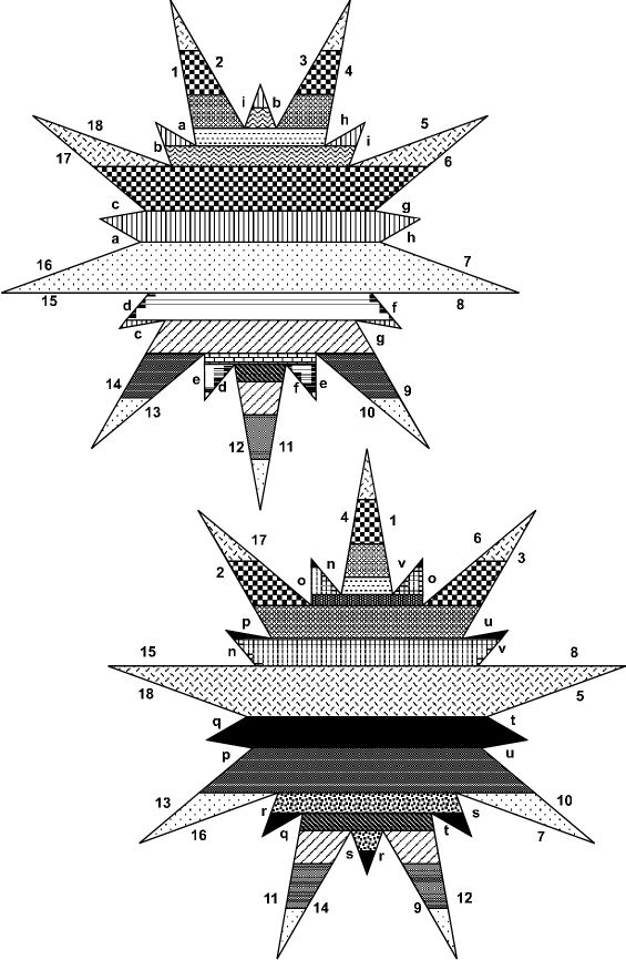
Figure 2. Cylinder decomposition of $X(5,9,\infty)$

Theorem 7.1.

Let $n\geq 7$ be odd and not divisible by $5$. Then the affine group of $X(5,n,\infty)$ contains the elements

$$R=\left(\begin{array}[]{cc}\cos(\pi/n)&-\sin(\pi/n)\\ \sin(\pi/n)&\cos(\pi/n)\end{array}\right)\quad\text{and}\quad T=\left(\begin{array}[]{cc}1&2\frac{\cos(\pi/n)+\cos(\pi/5)}{\sin(\pi/n)}\\ 0&1\end{array}\right).$$

The elements $R,T\in{\rm PSL}_{2}(\mathbb{R})$ generate the Fuchsian triangle group $\Delta(5,n,\infty)$. In particular, $X(5,9,\infty)$ is a Veech surface.

Proof: Rotation around the center of the stars defines an affine diffeomorphism of the surface $X(5,n,\infty)$. Its derivative is $R$.

We rotate $X(5,n,\infty)$ as in Figure 1 and Figure 2, i.e. such that the edge $I_{4}$ resp. the one with label $15$ is horizontal and to the left of the center of the star.

We now consider the horizontal foliation defined by $\omega$. Recall that a saddle connection is a leaf of the foliation that begins and ends in a singularity. In a dense set of directions, the saddle connections divide $X$ into metric cylinders, see for example [MaTa02], §4.1. We claim that in the horizontal direction $X$ decomposes into $g=2(n-1)$ metric cylinders. We distinguish two types of cylinders. Each cylinder corresponds to one shading style in Figure 2.

The cylinders of type $1$, denoted by $C_{i}$, are those that are glued together from pieces from both stars. An example is the checkered cylinder. Since the second star is obtained from the first by reflection, the cylinders $C_{i}$ appear in pairs, as can be seen from Figure 2. There is a bijection between the cylinders of type $1$ and pairs of long points. For example, the checkered cylinder corresponds to the long points $17$-$18$ and $5$-$6$. Here a ‘pair’ consists of an orbit of length $2$ of long points under the reflection in the vertical axis. The two vertical long points correspond to orbits of length one, and hence do not correspond to a cylinder of type $1$. We conclude that the number of cylinders of type $1$ is $n-1$.

The cylinders of the type $2$, denoted by $\widetilde{C}_{i}$, are those that consist of pieces of one star. An example is the black cylinder. These cylinders also come in pairs. There is a bijection between cylinders of type $2$ and pairs of short points. Therefore the number of cylinders of type $2$ is also $n-1$.

The width and the height of a pair of cylinders of type $1$, for an appropriate numbering, is given by

(15) $$\begin{split}w_{k}&=2|I_{3}|\cos\frac{(n-2k)\pi}{2n}\quad\text{and}\\ h_{k}&=|I_{4}|\left(\sin\frac{(n+1-2k)\pi}{2n}-\sin\frac{(n-1-2k)\pi}{2n}\right)=2|I_{4}|\sin\frac{\pi}{2n}\cos\frac{(n-2k)\pi}{2n}\end{split}$$

for $k=1,\ldots,(n-1)/2$. This is seen by cutting the points of the stars into pieces, and translating these pieces so that one obtains $2(n-1)$ connected cylinders, one for each shading style. One then uses the rotation and reflection symmetries of the original star.

Similarly, the widths and heights of pairs of cylinders $\widetilde{C}_{i}$, for an appropriate numbering, are given by

(16) $$\begin{split}\widetilde{w}_{k}&=2|I_{2}|\cos\frac{(n-2k)\pi}{2n}\quad\text{and}\\ \widetilde{h}_{k}&=|I_{1}|\left(\sin\frac{(n+2-2k)\pi}{2n}-\sin\frac{(n-2-2k)\pi}{2n}\right)=2|I_{1}|\sin\frac{2\pi}{2n}\cos\frac{(n-2k)\pi}{2n}\end{split}$$

for $k=1,\ldots,(n-1)/2$.

The moduli of these cylinders are

$$m_{k}:=h_{k}/w_{k}=|I_{4}|\sin\frac{\pi}{2n}/|I_{3}|\quad\text{and}\quad\widetilde{m}_{k}:=\widetilde{h}_{k}/\widetilde{w}_{k}=|I_{1}|\sin\frac{2\pi}{2n}/|I_{2}|.$$

Note that $m_{k}$ and $\widetilde{m}_{k}$ are independent of $k$.

We claim that $m_{k}/\widetilde{m}_{k}=|I_{4}||I_{2}|\sin(\pi/n)/|I_{3}||I_{1}|\sin(\pi/2n)=1$, that is that the moduli of all the cylinders are identical. This is equivalent to

(17) $$\frac{|I_{2}|}{|I_{1}|}=\frac{|I_{3}|}{|I_{4}|}\frac{\sin(\pi/n)}{\sin(\pi/2n)}.$$

Since we assumed that $I_{4}=1$, the right hand side is equal to $2|\mathop{\rm Re}(I_{3})|$.

Using the geometry of the billiard table one shows that

$$\begin{split}|I_{2}|\cos(3\pi/2n)&-|I_{1}|\cos(5\pi/2n)=|\mathop{\rm Re}(I_{3})|-|I_{4}|=|\mathop{\rm Re}(I_{3})|-1,\\ |I_{2}|\sin(3\pi/2n)&-|I_{1}|\sin(5\pi/2n)=\mathop{\rm Im}(I_{3})=\mathop{\rm Re}(I_{3})\tan(\pi/2n).\end{split}$$

This implies that

(18) $$\frac{|I_{2}|}{|I_{1}|}=\frac{-(\mathop{\rm Re}(I_{3})-1)\sin(5\pi/n)+\mathop{\rm Re}(I_{3})\tan(\pi/2n)\cos(5\pi/n)}{-(\mathop{\rm Re}(I_{3})-1)\sin(3\pi/n)+\mathop{\rm Re}(I_{3})\tan(\pi/2n)\cos(3\pi/n)}.$$

The minimal polynomial of $\mathop{\rm Re}(I_{3})$ over $\mathbb{Q}(\cos(\pi/n))$ is

(19) $$X^{2}-(2\cos(\pi/n)+1/2)X+(\cos^{2}(\pi/n)+\cos(\pi/n)/2-1/4).$$

One deduces (17) from (18), (19) and the addition laws for sines and cosines.

From the claim (17), we deduce that $T$ is contained in the affine group of $X$. Namely, fixing the horizontal lines and postcomposing local charts of the cylinders by $T$ defines an affine diffeomorphism whose derivative is $T$ (compare to [Ve89] Proposition 2.4 or [McM03] Lemma 9.7).

It remains to prove that $R$ and $T$ generate the $(5,n,\infty)$-triangle group. One constructs the hyperbolic triangle in the extended upper half plane with corners $i\infty,i$ and

$$z_{0}=\frac{\cos(\pi/n)+\cos(\pi/5)}{\sin(\pi/n)}+i\,\frac{\sin(\pi/5)}{\sin(\pi/n)}$$

bounded by the vertical axes through $i$ and $z_{0}$ and the circle around $\cot(\pi/n)$ with radius $1/\sin(\pi/n)$. The interior angles at $i$ and $z_{0}$ are indeed $\pi/n$ and $\pi/5$. By Poincaré’s Theorem this triangle plus its reflection along the imaginary axis is a fundamental domain for the group generated by $R$ and $T$.

The last claim follows now from the standard criterion to detect Teichmüller curves, see e.g. [McM03] Corollary 3.3. $\Box$

Remark 7.2.

Assuming the comparison results which will be proved in Section 7.3 below, the number of cylinders in, say, the horizontal direction is already determined by results of the previous sections.

Consider the family of translation surfaces ${\rm diag}(e^{t},e^{-t})\cdot(X_{0},\omega_{0})$, where $(X_{0},\omega_{0})$ is as in Theorem 5.15. This family converges for $t\to\infty$ to a singular fiber of $\overline{f}:\overline{{\mathcal{X}}}\to\overline{C}$ and by [Ma75] the number of cylinders in the horizontal direction equals the number of singularities of the singular fiber $X_{\infty}$.

Since all the local systems $\mathbb{L}_{i}$ as in the proof of Theorem 5.2 have non-trivial parabolic monodromy around points in $\overline{\pi}^{-1}(\infty)$ the arithmetic genus of $X_{\infty}$ is zero. Since $\omega_{0}$ has only one zero, $X_{\infty}$ is irreducible and hence the number of singularities of the fiber $X_{\infty}$ equals $g(X_{\infty})$.

7.2. The tables $T(4,n,\infty)$

Let $n\geq 5$ be odd. We define a billiard table $T{(4,n,\infty)}$ as follows. The billiard table is a again a $4$-gon in the complex plane with angles $\alpha=\pi/2$ and $\beta=\gamma=\pi/n$, as indicated in Figure 3. We denote by $I_{1},\ldots,I_{4}$ the vectors corresponding to the sides of the polygon. We regards these vectors as complex numbers.

Figure 3. Billiard table $T{(4,n,\infty)}$, for $n=9$

We scale and rotate the billiard table such that $I_{4}=1$ and such that $|I_{3}|=2(\cos(\pi/n)+\cos(\pi/4)).$ This determines the table uniquely.

The translation surface $X:=X(4,n,\infty)$ obtained by unfolding $T{(4,n,\infty)}$ looks similar to the one obtained from $T{(5,n,\infty)}$. It can be obtained by identifying parallel sides of two stars. The first star is illustrated in Figure 4. The second star is obtained from the first by reflection in the horizontal axis.

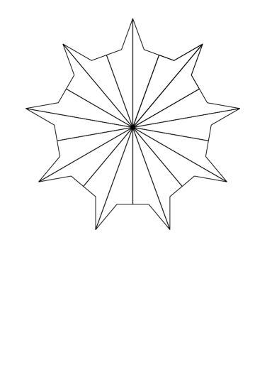
Figure 4. Billiard table $T{(4,9,\infty)}$, partially unfolded

The translation surface $X(4,n,\infty)$ has one singularity which corresponds to the vertex of the billiard table with angle $\delta$. Its genus is $g=3(n-1)/2$.

Theorem 7.3.

Let $n\geq 5$ be odd. Then the affine group of $X(4,n,\infty)$ contains the elements

$$R=\left(\begin{array}[]{cc}\cos(\pi/n)&-\sin(\pi/n)\\ \sin(\pi/n)&\cos(\pi/n)\end{array}\right)\quad\text{and}\quad T=\left(\begin{array}[]{cc}1&2\frac{\cos(\pi/n)+\cos(\pi/4)}{\sin(\pi/n)}\\ 0&1\end{array}\right).$$

The elements $R,T\in{\rm PSL}_{2}(\mathbb{R})$ generate the Fuchsian triangle group $\Delta(4,n,\infty)$. In particular, $X(4,9,\infty)$ is a Veech surface.

Proof: Rotation around the center of each of the stars defines an affine diffeomorphism of $X(4,n,\infty)$ whose derivative is $R$, as in the case $(5,n,\infty)$.

We describe the cylinders in the horizontal direction. As for $X(5,n,\infty)$, we distinguish two types of cylinders. The cylinders of type $1$, denoted by $C_{i}$, are those that are glued together from pieces of both stars. They correspond to pairs of sides which connect two points. Here a pair of sides consist of two distinct sides which are interchanged by reflection in the vertical axis. There are $(n-1)/2$ such cylinders. The widths and heights of these cylinders, in an appropriate numbering, are given by

$$w_{k}=4|I_{2}|\cos\left(\frac{(n-2k)\pi}{2n}\right)\quad\text{and}\quad h_{k}=2|I_{1}|\sin\left(\frac{k\pi}{n}\right),\qquad k=1,\ldots,(n-1)/2.$$

There are two cylinders with the same width and height, due to the symmetry.

The cylinders of type $2$, denoted by $\widetilde{C}_{i}$, are those that consist of pieces of one star only. They correspond to pairs of points of the stars. Here we use the same convention for pairs as above. The number of such cylinders is also $(n-1)/2$. The widths and heights of these cylinders are are

$$\begin{split}\widetilde{w}_{k}&=2|I_{3}|\cos\left(\frac{(n-2k+2)\pi}{2n}\right)\quad\text{and}\\ \widetilde{h}_{k}&=2|I_{4}|\cos\left(\frac{(n-2k+2)\pi}{2n}\right)\sin\left(\frac{\pi}{n}\right),\qquad k=1,\ldots,(n-1)/2.\end{split}$$

The moduli of the cylinders are

$$m_{k}:=h_{k}/w_{k}=|I_{1}|/2|I_{2}|\qquad\text{and}\qquad\widetilde{m}_{k}=\widetilde{h}_{k}/\widetilde{w}_{k}=|I_{4}|\sin\frac{\pi}{n}/|I_{3}|.$$

As in the proof of Theorem 7.1, one checks that $m_{k}/\widetilde{m}_{k}=|I_{1}||I_{3}|/2|I_{2}||I_{4}|\sin\left({\pi}/{n}\right)=1$, by using the geometry of the billiard table and the minimal polynomial of $2(\cos(\pi/n)+\cos(\pi/4))$ over $\mathbb{Q}(\cos(\pi/n))$. The rest of the proof is analogous to the proof of Theorem 7.1. $\Box$

7.3. Comparison with Theorems 5.2 and 5.15

In this section we relate the billiard tables constructed in §§7.1 and 7.2 to the families of curves constructed in §5. For simplicity we suppose that $1<m<n$ are relatively prime integers such that $n$ is odd. This assumption avoids a case distinction. It is easy to work out the general statement.

In Theorem 5.2 we constructed a Teichmüller curve with projective affine group $\Delta(m,n,\infty)$. We constructed a concrete finite cover, $C$, of this Teichmüller curve. We denote by $\overline{C}$ the corresponding projective curve. Over $\overline{C}$ there exists a universal family $f:\overline{{\mathcal{X}}}\to\overline{C}$ of semistable curves. In Theorem 5.15 we showed that there exist points $c$ of $\overline{C}$ such that the fiber $X_{0}:={\mathcal{X}}_{c}$ is a smooth curve which is a $2n$-cyclic cover of the projective line branched at $(m+3)/2$ (resp. $(m+4)/2$) points if $m$ is odd (resp. even). There also exist fibers of ${\mathcal{X}}$ which are $2m$-cyclic covers of the projective line branched at $(n+3)/2$, but we do not regard these here since it is convenient to have as few branch points as possible, for our purposes. One may check that this is the most efficient way to represent a fiber of ${\mathcal{X}}$ as an abelian cover of the projective line. This representation allows us to use Schwarz–Christoffel maps ([Wa98] Theorem C’) to represent the fiber $X_{0}$ of ${\mathcal{X}}$ as the unfolding of a billiard table, under certain conditions (see below).

We first suppose that $m$ is odd. The $2n$-cyclic cover $X_{0}\to\mathbb{P}^{1}_{u}$ of Theorem 5.15.(a) is branched at the real points $2\cos(2k\pi/m)$. The Schwarz–Christoffel map is defined as

$$SC(w)=\int_{0}^{w}(u-2)^{\frac{1}{2n}-1}\prod_{k=1}^{(m-1)/2}(u-2\cos(2k\pi/m))^{\frac{1}{n}-1}\,{\rm d}u.$$

The integrand is the generating differential form $\omega_{0}$.

The Schwarz–Christoffel map maps the real axis to a $(m+3)/2$-gon which we denote by $T[m,n,\infty]$. If $T[m,n,\infty]$ has no self-crossings then $SC$ maps the upper half-plane bijectively to the interior of this $(m+3)/2$-gon. The interior angles of $T[m,n,\infty]$ are $(m-1)/2$ times $\pi/n$ and once $\pi/2n$, in this order. The remaining angle is $2\pi-m\pi/2n\bmod 2\pi$ (resp. $\pi-m\pi/2n$) if $m\equiv 1\bmod{4}$ (resp. $m\equiv 3\bmod{4}$). The number of self-crossings is therefore $(m-5)/4$ if $m\equiv 1\bmod{4}$ and $(m-3)/4$ if $m\equiv 3\bmod{4}$. In particular, this number is zero if and only if $m=3,5$. For $m\geq 7$ it therefore unclear whether one can obtain $(X_{0},\omega_{0})$ by unfolding a billiard table. However, it follows from our results that one cannot do this via the usual theory of Schwarz–Christoffel maps. Namely, for $m\geq 7$ one cannot represent a smooth fiber of $\overline{{\mathcal{X}}}$ as a cyclic cover of the projective line, such that the corresponding polygon does not have self-crossings.

If $m=3$ or $5$, Theorem C’ of [Wa98] implies that the Veech surface $(X_{0},\omega_{0})$ is obtained by unfolding the billiard table $T[m,n,\infty]$. For $m=3$, we obtain Ward’s family (compare to Theorem 5.15.(c)). For $m=5$, the angles of the $4$-gon $T[5,n,\infty]$ coincide with those of the billiard table $T(5,n,\infty)$ which we constructed in §7.1. We show below that both $4$-gons are similar.

The case that $m$ even is analogous. The Schwarz–Christoffel map

$$SC(w)=\int_{0}^{w}(u-2)^{\frac{1}{2}-1}\prod_{k=1}^{m/2}(u-2\cos((2k-1)\pi/2m))^{\frac{1}{n}-1}\,{\rm d}u$$

maps the real axis to a $(m+4)/2$-gon $T[m,n,\infty]$. The interior angles of $T[m,n,\infty]$ are once $\pi/2$ and $m/2$ times $\pi/n$, in this order. The remaining angle is $(3n-m)\pi/2n$ if $m\equiv 0\bmod{4}$ and $((n-m)\pi/(2n)$ if $m\equiv 2\bmod{4}$. We conclude that the number of self-crossings is $(m-4)/4$ (resp. $(m-2)/4$) if $m\equiv 0\bmod{4}$ (resp. $m\equiv 2\bmod{4}$). Therefore the number of self-crossings is zero if and only if $m=2,4$. The case $m=2$ corresponds to Veech’s family [Ve89] (§4). We show below that the case $m=4$ corresponds to the billiards constructed in §7.2.

We leave it to the reader to use Theorem 5.2 and the techniques of Theorem 5.15 to construct billiard tables with projective affine group $\Delta(4,n,\infty)$ and $\Delta(5,n,\infty)$ also in the case that $n$ even or divisible by $5$, or both.

Proposition 7.4.

Let $m$ be either $4$ or $5$. The billiard table $T[m,n,\infty]$ is similar to the billiard table $T{(m,n,\infty)}$.

Proof: Suppose that $m=5$. The case that $m=4$ is similar, and left to the reader.

Recall that the interior angles of the $4$-gons $T(5,n,\infty)$ and $T[5,n,\infty]$ are the same, and also occur in the same order. Therefore we only have to compare the lengths of the sides of $T[5,n,\infty]$ to those of $T(5,m,\infty)$. Since the sides of $T[5,n,\infty]$ are expressed in terms of the Schwarz–Christoffel map, it suffices to show that

(20) $$\frac{|SC(2\cos(2\pi/5))-SC(2)|}{|SC(\infty)-SC(2)|}=\frac{|I_{3}|}{|I_{4}|}=\frac{\cos(\pi/n)+\cos(\pi/5)}{\cos(\pi/2n)}.$$

Here $I_{3},I_{4}$ are the vectors corresponding to the sides of the $4$-gon $T[5,n,\infty]$ as indicated in Figure 1.

We first express the length of the vector $I_{4}$ in terms of Beta integrals:

(21) $$\begin{split}|I_{4}|&=\int_{2}^{\infty}(u-2)^{\frac{1}{2n}-1}(u-2\cos(2\pi/5))^{\frac{1}{n}-1}(u-2\cos(4\pi/5))^{\frac{1}{n}-1}\,{\rm d}u\\ &=\int_{1}^{\infty}z^{1-\frac{5}{2n}}(z^{5}-1)^{\frac{1}{n}-1}(z+1)\,{\rm d}z.\end{split}$$

Here we used the substitution $u=z+1/z$, compare to the proof of Theorem 5.15. Substituting $z=1/t$, we recognize this integral as the sum of two Beta integrals:

(22) $$|I_{4}|=\frac{1}{5}\left(\mathop{\rm B}(\frac{2}{5}-\frac{1}{2n},\frac{1}{n})+\mathop{\rm B}(\frac{3}{5}-\frac{1}{2n},\frac{1}{n})\right).$$

Similarly, one finds that

(23) $$|I_{3}|=\frac{1}{5}\left((-1+\zeta_{5}^{2}\zeta_{2n}^{-1})\mathop{\rm B}(\frac{2}{5}-\frac{1}{2n},\frac{1}{n})+(-1+\zeta_{5}^{3}\zeta_{2n}^{-1})\mathop{\rm B}(\frac{3}{5}-\frac{1}{2n},\frac{1}{n})\right).$$

Equation (20) follows from (22) and (23) by expressing the Beta integrals in terms of Gamma functions, using that $\Gamma(z)\Gamma(1-z)=\pi/\sin(\pi z)$, and applying the addition formulas for sines and cosines. $\Box$

One may give an alternative proof for the statement that the $4$-gons $T[5,n,\infty]$ and $T(5,n,\infty)$ are similar by showing the following. Let $P$ be any $4$-gon with the prescribed angles, and let $X$ be the corresponding translation surface. Suppose that the affine group of $X$ contains $R$ and $T$. Then $P$ is similar to $T(5,n,\infty)$. This can be shown by first deducing from the geometry of $P$ that an affine diffeomorphism with derivative $R$ has to fix each saddle connection.

Remark 7.5.

Several authors ([Wa98], [Vo96], [KeSm00], [Pu01]) have classified the Teichmüller curves that are obtained by unfolding a rational triangle, under certain conditions on the angles of the triangle. We have obtained the translation surfaces $X(m,n,\infty)$ for $m=4,5$ by unfolding $4$-gons. The corresponding families of Teichmüller curves have not been found by Ward et. al. This suggests that the translation surfaces $X(m,n,\infty)$ for $m=4,5$ may not be obtained by unfolding triangles, but of course we have not shown this.

Remark 7.6.

For $n>m\geq 6$ we have not been able to obtain the translation surface $X(m,n,\infty)$ by unfolding a billiard table, since the corresponding polygon $T[m,n,\infty]$ may not be embedded in the complex plane. However, it should in principle be possible to give a concrete description of $X(m,n,\infty)$ as obtained by gluing certain cylinders, analoguous to the description in the case of $m=4,5$ (§§7.1, 7.2). As for $m=4$ and $5$, it follows from Corollary 5.9 that we would need $g(X_{0})$ cylinders, which is approximately $(m-1)(n-1)/2$: it will be difficult to visualize the result. Therefore it seems more natural to us to represent these Teichmüller curves via the algebraic description from §5.

8. Lyapunov exponents

Roughly speaking, a flat normed vector bundle on a manifold with a flow, i.e. an action of $\mathbb{R}^{+}$, can sometimes be stratified according to the growth rate of the length of vectors under parallel transport along the flow. The growth rates are then called Lyapunov exponents. In this section we will relate Lyapunov exponents to degrees of some line bundles in case that the underlying manifold is a Teichmüller curve.
For the convenience of the reader we reproduce Oseledec’s theorem ([Os68]) that proves the existence of such exponents. We give a restatement due to [Ko97] in a language closer to our setting.

8.1. Multiplicative ergodic theorem

We start with some definitions. A measurable vector bundle is a bundle that can be trivialized by functions which only need to be measurable. If $(V,||\cdot||)$ and $(V^{\prime},||\cdot||)$ are a normed vector bundles and $T:V\to V^{\prime}$, then we let $||T||:=\sup_{||v||=1}||T(v)||$. A reference for notions in ergodic theory is [CFS82].

Theorem 8.1 (Oseledec).

Let $T_{t}:(M,\nu)\to(M,\nu)$ be an ergodic flow on a space $M$ with finite measure $\nu$. Suppose that the action of $t\in\mathbb{R}^{+}$ lifts equivariantly to a flow $S_{t}$ on some measurable real bundle $V$ on $M$. Suppose there exists a (not equivariant) norm $||\cdot||$ on $V$ such that for all $t\in\mathbb{R}^{+}$

$$\int_{M}\log(1+||S_{t}||)\nu<\infty.$$

Then there exist real constants $\lambda_{1}\geq\cdots\geq\lambda_{k}$ and a filtration

$$V=V_{\lambda_{1}}\supset\cdots V_{\lambda_{k}}\supset 0$$

by measurable vector subbundles such that, for almost all $m\in M$ and all $v\in V_{m}\smallsetminus\{0\}$, one has

$$||S_{t}(v)||={\rm exp}(\lambda_{i}t+o(t)),$$

where $i$ is the maximal value such that $v\in(V_{i})_{m}$.
The $V_{\lambda_{i}}$ do not change if $||\cdot||$ is replaced by another norm of ‘comparable’ size (e.g. if one is a scalar multiple of the other).

The numbers $\lambda_{i}$ for $i=1,\ldots,k\leq{\rm rank}(V)$ are called the Lyapunov exponents of $S_{t}$. Note that these exponents are unchanged if we replace $M$ by a finite unramified covering with a lift of the flow and the pullback of $V$. We adopt the convention to repeat the exponents according to the rank of $V_{i}/V_{i+1}$ such that we will always have $2g$ of them, possibly some of them equal. A reference for elementary properties of Lyapunov exponents is e.g. [BGGS80].

If the bundle $V$ comes with a symplectic structure the Lyapunov exponents are symmetric with respect to $0$, i.e. they are ([BGGS80] Prop. 5.1)

$$1=\lambda_{1}\geq\lambda_{2}\geq\cdots\geq\lambda_{g}\geq 0\geq-\lambda_{g}\geq\cdots\geq-\lambda_{1}=-1.$$

We specialize these concepts to the situation we are interested in. Let $\Omega M_{g}^{*}$ be the bundle of non-zero holomorphic $1$-forms over the moduli space of curves. Its points are translation surfaces. The $1$-forms define a flat metric on the underlying Riemann surface and we let $\Omega_{1}M_{g}\subset\Omega M_{g}^{*}$ be the hypersurface consisting of translation surfaces of area one. As usual we replace $M_{g}$ by an appropriate fine moduli space adding a level structure, but we do not indicate this in the notation. This allows us to use a universal family $f:{\mathcal{X}}\to M_{g}$.
Over $\Omega_{1}M_{g}$, we have the local system $\mathbb{V}_{\mathbb{R}}=R^{1}f_{*}\mathbb{R}$, whose fiber over $(X,\omega)$ is $H^{1}(X,\mathbb{R})$. We denote the corresponding real $C^{\infty}$-bundle by $V$. This bundle naturally carries the Hodge metric

$$H(\alpha,\beta)=\int_{X}\alpha\wedge*\beta,$$

where classes in $H^{1}(X,\mathbb{R})$ are represented by $\mathbb{R}$-valued $1$-forms, and where $*$ is the Hodge star operator. We denote by $||\cdot||:=||\cdot||_{T}$ the associated metric on $V$.
There is a natural ${\rm SL}_{2}(\mathbb{R})$-action on $\Omega_{1}M_{g}$ obtained by post-composing the charts given by integrating the $1$-form with the $\mathbb{R}$-linear map given by $A\in{\rm SL}_{2}(\mathbb{R})$ to obtain a new complex structure and new holomorphic $1$-form (see e.g.  [McM03] and the reference there). The geodesic flow $T_{t}$ on $\Omega_{1}M_{g}$ is the restriction of the ${\rm SL}_{2}(\mathbb{R})$-action to the subgroup ${\rm diag}(e^{t},e^{-t})$. Since $V$ carries a flat structure, we can lift $T_{t}$ by parallel transport to a flow $S_{t}$ on $V$. This is the Kontsevich–Zorich cocycle. The notion ‘cocycle’ is motivated by writing the flow on a vector bundle in terms of transition matrices.

Lyapunov exponents can be studied for any finite measure $\nu$ on a subspace $M$ of $\Omega_{1}M_{g}$ such that $T_{t}$ is ergodic with respect to $\nu$. Starting with the work of Zorich ([Zo96]), Lyapunov exponents have been studied for connected components of the stratification of $\Omega_{1}M_{g}$ by the order of zeros of the $1$-form. The integral structure of $\Omega M_{g}^{*}$ as an affine manifold can be used to construct a finite ergodic measure $\mu$. Lyapunov exponents for $(\Omega_{1}M_{g},\mu)$ may be interpreted as deviations from ergodic averages of typical leaves of measured foliations on surfaces of genus $g$. The reader is referred to [Ko97], [Fo02] and the surveys [Kr03] and [Fo05] for further motivation and results.

8.2. Lyapunov exponents for Teichmüller curves

We want to study Lyapunov exponents in case of an arbitrary Teichmüller curve $C$ or rather its canonical lift $M$ to $\Omega_{1}M_{g}$ given by providing the Riemann surfaces parameterized by $C$ with the normalized generating differential. The lift $\pi:M\to C$ is an $S^{1}$-bundle. We equip $M$ with the measure $\nu$ which is induced by the Haar measure on ${\rm SL}_{2}(\mathbb{R})$, normalized such that $\nu(M)=1$. Locally, $\nu$ is the product of the measure $\nu_{C}$ coming from the Poincaré volume form and the uniform measure on $S^{1}$, both normalized to have total volume one.
We can apply Oseledec’s theorem since $\nu_{M}$ is ergodic for the geodesic flow ([CFS82] Theorem 4.2.1).

We start from the observation that the decomposition $(\ref{VHSdecomp})$ of the VHS in Theorem 1.1 is ${\rm SL}_{2}(\mathbb{R})$-equivariant and orthogonal with respect to Hodge metric. This implies that the Lyapunov exponents of $\mathbb{V}$ are the union of the Lyapunov exponents of the $\mathbb{L}_{i}$ with those of $\mathbb{M}$.

Let ${\mathcal{L}}_{i}:=(\mathbb{L}_{i})^{1,0}$ be the $(1,0)$-part of the Hodge filtration of the Deligne extension of $\mathbb{L}_{i}$ to $\overline{C}$. Denote by $d_{i}:=\deg({\mathcal{L}}_{i})$ the corresponding degrees. Recall from Theorem 1.1 that precisely one of the $\mathbb{L}_{i}$, say the first one $\mathbb{L}_{1}$ is maximal Higgs. Recall that $S=\overline{C}\smallsetminus C$ is the set of singular fibers.

Theorem 8.2.

Let $\nu_{M}$ be the finite ${\rm SL}_{2}(\mathbb{R})$-invariant measure with support in the canonical lift $M$ of a Teichmüller curve to $\Omega_{1}M_{g}$. Then $r$ of the Lyapunov exponents $\lambda_{i}$ satisfy

$$\lambda_{i}=d_{i}/d_{1}=\lambda(\mathbb{L}_{i},S).$$

In particular, these exponents are rational, non-zero and their denominator is bounded by $2g-2+s$, where $s=|S|$.

Proof: We write $(\mathbb{L}_{i})_{\mathbb{R}}$ for the local subsystem of $R^{1}f_{*}\mathbb{R}$ such that $(\mathbb{L}_{i})_{\mathbb{R}}\otimes_{\mathbb{R}}\mathbb{C}=\mathbb{L}_{i}$ and let $L_{i}$ be the $C^{\infty}$-bundle attached to $(\mathbb{L}_{i})_{\mathbb{R}}$. We apply Oseledec’s theorem to $L_{i}$. Then

$$\lambda_{i}=\lim_{t\to\infty}\frac{1}{t}\log||S_{t}(v_{i})||,$$

for $v_{i}\in L_{i}\smallsetminus(L_{i})_{-\lambda_{i}}$. By averaging, we have

$$\lambda_{i}=\lim_{t\to\infty}\frac{1}{t}\int_{G(L_{i})}\log||S_{t}(v_{i})||{\rm d}\nu_{G(L_{i})(v_{i})},$$

where $\tau:G(L_{i})\to M$ is the (Grassmann) bundle of norm one vectors in $L_{i}$. This bundle is locally isomorphic to $S^{1}\times M$. The measure $\nu_{G(L_{i})}$ is locally the product measure of $\nu$ with the uniform measure on $S^{1}$.

Following the idea of Kontsevich ([Ko97]) also exploited in Forni ([Fo02]), we estimate the growth of the length of $v_{i}$ not only as a function on the $T_{t}$-ray through $\tau(v_{i})$ (given as the parallel transport of the corresponding vector) but as a function on the whole (quotient by a discrete group of a) Poincaré disc $D_{\tau(v_{i})}$ in $M$. For this purpose we write $z=e^{i\theta}r$ ($\theta\in[0,2\pi))$ for $z$ in the unit disc $D$ and lift it to $\rho_{\theta}\,{\rm diag}(e^{t},e^{-t})\in{\rm SL}_{2}(\mathbb{R})$, where $\rho_{\theta}$ is the rotation matrix by $\Theta$ and $t=(1/2)\log((1+r)/(1-r))$. Using this lift $D\to{\rm SL}_{2}(\mathbb{R})$ we obtain our disc $D_{\tau(v_{i})}$ in $M$ using the (left) ${\rm SL}_{2}(\mathbb{R})$-action on $M$.
Consider the following functions

$$f_{D}:=f_{D,i}:\left\{\begin{array}[]{lcl}(\pi^{*}L_{i}\smallsetminus\{0\})\times D&\longrightarrow&\mathbb{R}\\ (v_{i},z)&\mapsto&\log||z\cdot v_{i}||,\end{array}\right.$$

where $z\cdot v_{i}$ is the parallel transport of $v_{i}$ over the disc $D_{\tau(v_{i})}$. This is well-defined since the monodromy of $L_{i}$ acts by matrices in ${\rm SL}_{2}(\mathbb{Z})={\rm Sp}_{2}(\mathbb{Z})$ and symplectic transformations do not affect the Hodge length. Note that by definition

(24) $$f_{D}(v_{i},z)=f_{D}(z\cdot v_{i},0).$$

On the discs $D_{\tau(v_{i})}$ we may apply the (hyperbolic) Laplacian $\Delta_{h}$ to the functions $f_{D_{\tau(v_{i})}}$ with respect to the second variable, i.e. consider

$$h_{D}:=h_{D,i}:\left\{\begin{array}[]{lcl}(\pi^{*}L_{i}\smallsetminus\{0\})\times D&\longrightarrow&\mathbb{R}\\ (v_{i},z)&\mapsto&(\Delta_{h}f_{D}(v_{i},\cdot))(z).\end{array}\right.$$

Using (24) and the invariance of $\Delta_{h}$ under isometries one deduces that there is a function $h:\pi^{*}L_{i}\smallsetminus\{0\}\to\mathbb{R}$, such that

(25) $$h_{D}(v_{i},z)=h(z\cdot v_{i}).$$

Since obviously $\int_{G(L_{i})}h(S_{t}v_{i}){\rm d}\nu_{G(L_{i})}(v_{i})=\int_{G(L_{i})}h(v_{i}){\rm d}\nu_{G(L_{i})}(v_{i})$ for any $t$, we can apply [Kr03] Equation (3) (see also [Fo02] Lemma 3.1) to obtain

(26) $$\lambda_{i}=\int_{G(L_{i})}h(v_{i})\nu_{G(L_{i})}(v_{i}).$$

We want to relate this expression to the degree $d_{i}$ of the line bundles ${\mathcal{L}}_{i}$. Suppose $s_{i}(u)$ is a holomorphic section of ${\mathcal{L}}_{i}$ over some open $U\subset C$. Recall that $L_{i}$ has unipotent monodromies, by assumption. Therefore [Pe84] Proposition 3.4 implies that the Hodge metric grows not too fast near the punctures and we have

(27) $$d_{i}=\frac{1}{2\pi i}\int_{\overline{C}}\partial\overline{\partial}\log(||s_{i}||).$$

Here as usual, if there is no global section of ${\mathcal{L}}_{i}$ the contributions of local holomorphic sections are added up using a partition of unity.

Instead of considering a holomorphic section $s_{i}$, we now consider a flat section $v_{i}(u)$ of $L_{i}$ over $U$. Then, in $(\wedge^{2}(\mathbb{L}_{i})_{\mathbb{C}})^{\otimes 2}(U)$ one checks the identity

(28) $$(v_{i}\wedge*v_{i})\otimes(s_{i}\wedge\overline{s_{i}})=\frac{1}{2}(v_{i}\wedge s_{i})\otimes(v_{i}\wedge\overline{s_{i}}).$$

We integrate this identity over the fibers ${\mathcal{X}}_{c}$ of $f:{\mathcal{X}}\to C$, take logarithms and the Laplacian $\frac{1}{2\pi i}\partial\overline{\partial}$. Note that

(29) $$\frac{1}{2\pi i}\partial\overline{\partial}\log\frac{1}{2}(v_{i}\wedge s_{i})\otimes(v_{i}\wedge\overline{s_{i}})=0.$$

Let $F$ be a fundamental domain for the action of the affine group $\Gamma$ in a Poincaré discs $D\hookrightarrow M$. Then (27) and (29) implies that for any flat section $v_{i}$ of $L_{i}$ we have

$$d_{i}=\frac{-1}{2\pi i}\int_{F}\partial\overline{\partial}\log(||v_{i}||).$$

The differential operator $\partial\overline{\partial}$ coincides, up to a scalar, with $\Delta_{h}(\cdot)\omega_{P}$, where $\omega_{P}$ is the Poincaré area form. Therefore we obtain for each $v_{i}\in(\pi\circ\tau)^{*}(L_{i}\smallsetminus\{0\})$ that

$$d_{i}=\frac{1}{4\pi}\int_{F}\Delta_{h}\log||v_{i}(z)||\omega_{P}(z),$$

where $v_{i}(z)$ is obtained from $v_{i}$ via parallel transport. Hence by integrating over all $G(L_{i})$ and taking care of the normalization of $\nu_{G(L_{i})}$ we find that

(30) $$d_{i}=\frac{1}{4\pi}{\rm vol}(C)\int_{G(L_{i})}\Delta_{h}\log||v_{i}||\nu_{G(L_{i})(v_{i})}$$

The statement of the theorem now follows by comparing (30) with (26). $\Box$

Corollary 8.3.

At least $r$ of the Lyapunov exponents are non-zero.

Proof: By Theorem 8.2, it is sufficient to show that for ${\mathcal{L}}_{i}:=(\mathbb{L}_{i})^{(1,0)}$ the degree $\deg({\mathcal{L}}_{i})\neq 0$. If ${\mathcal{L}}_{i}=0$ then, by Simpson’s correspondence ([ViZu04] Theorem 1.1), $\mathbb{L}_{i}$ would be a reducible local system. But since $\mathbb{L}_{i}$ is Galois conjugate to $\mathbb{L}_{1}$, this is a contradiction. $\Box$.

Remark 8.4.

If $r\geq g-1$ all the Lyapunov exponents are known. In fact in this case we can identify the remaining Lyapunov exponent by the formula ([Ko97], [Fo02] Lemma 5.3)

$$\sum_{i=1}^{g}\lambda_{i}=\frac{\deg(f_{*}\omega_{X/C})}{2g-2+s}$$

In the case of Teichmüller curves associated with triangle groups constructed in §4 and §5, the proof of Theorem 8.2 yields more. Since for these curves the VHS decomposes completely into subsystems of rank two (Remark 5.11) we can determine all the Lyapunov exponents.

Proposition 8.5.

Suppose the local system $\mathbb{M}$ as in Theorem 1.1 contains a rank two local subsystem $\mathbb{F}_{i}$, whose $(1,0)$-part is a line bundle, which denote by ${\mathcal{F}}_{i}$. Then the Lyapunov spectrum contains (in addition to the $d_{i}/d_{1}$) the exponents

$$\deg({\mathcal{F}}_{i})/d_{1}.$$

By Theorem 8.2 and Proposition 8.5 it is justified to call $\lambda(\mathbb{L}_{i})$ Lyapunov exponents.

Irene I. Bouw Martin Möller
Mathematisches Institut FB 6 (Mathematik), Campus Essen
Heinrich-Heine-Universität Universität Duisburg-Essen
40225 Düsseldorf 45117 Essen
bouw@math.uni-duesseldorf.de martin.moeller@uni-essen.de

References

- [BGGS80] Benettin, G., Galgini, I., Giorgilli, A., Strelcyn, J.-M., Lyapunov characteristic exponents for smooth dynamical systems and for Hamiltonian systems; a method for computing all of them, Part I, Meccanica (1980), 9–20
- [Bo01] Bouw, I. I., The -rank of ramified covers of curves, Compositio Math. 126 (2001), 295–322
- [Bo04] Bouw, I. I., Reduction of the Hurwitz space of metacyclic covers, Duke Math. J. 121 (2004), 75–111
- [Bo05] Bouw, I., Pseudo-elliptic bundles, deformation data and the reduction of Galois covers, Habilitation thesis, Essen (2005)
- [BoWe05a] Bouw, I. I., Wewers, S., Alternating groups as monodromy groups in positive characteristic, Pacific J. of Math. 222 (2005), 185–199
- [BoWe05b] Bouw, I., Wewers, S., Indigenous bundles with nilpotent -curvature, preprint (2005), to appear in Internat. Math. Res. Notices.
- [CoWo90] Cohen, P., Wolfart, J., Modular embeddings for some non-arithmetic Fuchsian groups, Acta Arithm. 56 (1990), 93–110
- [CFS82] Cornfeld, I., Formin, S., Sinai, Y., Ergodic theory, Grundlehren der Mathematik 245, Springer (1982)
- [De70] Deligne, P., Equations différentielles à points singuliers réguliers, LNM 163, Springer (1970)
- [De87] Deligne, P., Un théorème de finitude pour la monodromie, in: Discrete groups in geometry and analysis, Progress in Math. 67, Birkhäuser (1987), 1–19
- [Fo02] Forni, G., Deviation of ergodic measures for area-preserving flows on surfaces, Ann. of Math. 155 (2002), 1–103
- [Fo05] Forni, G., On the Lyapunov exponents of the Kontsevich–Zorich cocycle, preprint (2005)
- [HaSt99] Harbater, D., Stevenson, K., Patching and thickening problems, J. of Algebra 212 (1999), 272–304
- [HuSc01] Hubert, P., Schmidt, T.A., Invariants of translation surfaces, Ann. Inst. Fourier 51 (2001), 461–495
- [Ka70] Katz, N.M., Nilpotent connections and the monodromy theorem: applications of a results of Turrittin, Inst. Hautes Études Sci. Publ. Math. 39 (1070), 355–412
- [KeSm00] Kenyon, R., Smillie, J., Billiards on rational-angled triangles, Comm. Math. Helv. 75 (2000), 65–108
- [KMS86] Kerkhoff, S., Masur, H., Smillie, J., Ergodicity of billiard flows and quadratic differentials, Ann. of Math. 124 (1986), 293–311
- [Ko97] Kontsevich, M., Lyapunov exponents and Hodge theory, The mathematical beauty of physics, in: Adv. Ser. Math. Phys. Vol. 24, World Scientific (1997) 318–332
- [Kr03] Krikorian, R., Déviations de moyennes ergodiques, flots de Teichmüller et cocycle de Kontsevich–Zorich, Sém. Bourbaki 927 (2003), to appear in Astérisque
- [Lo05] Lochak, P., On arithmetic curves in the moduli space of curves, J. Inst. Math. Jussieu 4 (2005), 449–503
- [Ma91] Margulis, G., Discrete subgroups of semisimple Lie groups, Springer (1991)
- [Ma75] Masur, H., On a class of geodesics in Teichmüller space, Annals of Math. 102 (1975), 205–221
- [MaTa02] Masur, H., Tabachnikov, S., Rational billiards and flat structures, in: Handbook of dynamical systems, vol. 1A, 1015–1089, Noth-Holland (2002).
- [McM03] McMullen, C., Billiards and Teichmüller curves on Hilbert modular sufaces, J. Amer. Math. Soc. 16 (2003), 857–885
- [McM04] McMullen, C., Teichmüller curves in genus two: Torsion divisors and ratios of sines, preprint (2004), to appear in Invent. Math.
- [McM05] McMullen, C., Prym varieties and Teichmüller curves, preprint (2005), to appear in Duke Math. Journal
- [Mo99] Mochizuki, S., Foundations of -adic Teichmüller theory, in: Studies in Adv. Math. No. 11, AMS/IP (1999)
- [Mö04] Möller, M., Periodic points on Veech surfaces and the Mordell–Weil group over a Teichmüller curve, preprint (2004), to appear in Invent. Math.
- [Mö06] Möller, M., Variations of Hodge structures of Teichmüller curves, J. Amer. Math. Soc. 19 (2006), 327–344
- [Os68] Oseledec, V. I., A multiplicative ergodic theorem. Lyapunov characteristic numbers for dynamical systems, Trans. Moscow Math. Soc. 19 (1968), 197–231
- [Pe84] Peters, C., A criterion for flatness of Hodge bundles over curves and Geometric Applications, Math. Ann. 268 (1984), 1–20
- [Pu01] Puchta, J.-C., On triangular billiards, Comment. Math. Helv. 76 No. 3 (2001), 501–505
- [Si72] Singerman, D., Finitely maximal Fuchsian groups, J. London Math. Soc. Ser. II (1972), 29–38
- [Ta77] Takeuchi, K., Arithmetic triangle groups, J. Math. Soc. Japan 29 (1977), 91–106
- [Ve89] Veech, W., Teichmüller curves in moduli space, Eisenstein series and an application to triangular billiards, Invent. Math. 97 (1989), 533–583
- [ViZu04] Viehweg, E., Zuo, K., A characterization of Shimura curves in the moduli stack of abelian varieties, J. of Diff. Geometry 66 (2004), 233–287
- [Vo96] Vorobets, Y. B., Plane structures and billiards in rational polygons: the Veech alternative, Russ. Math. Surveys 51 (1996), 779–817
- [Wa98] Ward, C., Calculation of Fuchsian groups associated to billiards in a rational triangle, Ergod. Th. and Dyn. Systems 18 (1998), 1019–1042
- [We99] Wewers, S., Deformation of tame admissible covers of curves, in: Aspects of Galois theory (1996), Lecture Note Ser. 256, London Math. Soc. (1999), 239–282
- [We98] Wewers, S., Construction of Hurwitz spaces, Thesis, Preprint No. 21 of the IEM, Essen (1998)
- [Yo87] Yoshida, M., Fuchsian differential equations. With special emphasis on the Gauss–Schwarz theory, Aspects of Math. 11 Vieweg (1987)
- [Zo96] Zorich, A., Finite Gauss measure on the space of interval exchange transformations. Lyapunov exponents, Ann. Inst. Fourier 46 (1996), 325–370