Flat fronts in hyperbolic 3-space
and their caustics

Abstract.

After Gálvez, Martínez and Milán discovered a (Weierstrass-type) holomorphic representation formula for flat surfaces in hyperbolic $3$-space $H^{3}$, the first, third and fourth authors here gave a framework for complete flat fronts with singularities in $H^{3}$. In the present work we broaden the notion of completeness to weak completeness, and of front to p-front. As a front is a p-front and completeness implies weak completeness, the new framework and results here apply to a more general class of flat surfaces.

This more general class contains the caustics of flat fronts — shown also to be flat by Roitman (who gave a holomorphic representation formula for them) — which are an important class of surfaces and are generally not complete but only weakly complete. Furthermore, although flat fronts have globally defined normals, caustics might not, making them flat fronts only locally, and hence only p-fronts. Using the new framework, we obtain characterizations for caustics.

1. Introduction

For an arbitrary Riemannian $3$-manifold $N^{3}$, a $C^{\infty}$-map

$$f\colon{}M^{2}\longrightarrow N^{3}$$

from a $2$-manifold $M^{2}$ is a (wave) front if $f$ lifts to a smooth immersed section

$$L_{f}\colon{}M^{2}\longrightarrow T_{1}N^{3}(\approx T_{1}^{*}N^{3})$$

of the unit tangent vector bundle $T_{1}N^{3}$ such that $df(X)$ is perpendicular to $L_{f}(p)$ for all $X\in T_{p}M^{2}$ and $p\in M^{2}$. Fronts generalize immersions, as they allow for singularities. The lift $L_{f}$ can be viewed as a globally defined unit normal vector field of $f$. However, global definedness of $L_{f}$ can be a stronger condition than desired. Sometimes p-fronts are more appropriate: The map $f$ is called a p-front if for each $p\in M^{2}$, there is a neighborhood $U$ of $p$ such that the restriction $f|_{U}$ is a front. The projectified cotangent bundle $P(T^{*}N^{3})$ has a canonical contact structure, and a p-front can be considered as the projection of a Legendrian immersion of $M^{2}$ into $P(T^{*}N^{3})$. A p-front $f$ is a front if and only if there exists a globally defined unit normal vector field, in which case we say $f$ is co-orientable. Otherwise, $f$ is non-co-orientable.

& (a) (b)

Figure 1. A flying saucer front and toroidal p-front.

For example, Figure 1 (a) is a plane curve front with a globally defined unit normal vector field. On the other hand, Figure 1 (b) is the limaçon, whose unit normal vector field is not single-valued on the curve. Rotating the first curve about its central vertical axis gives a surface like a “flying saucer”, which is a front in Euclidean space $\boldsymbol{R}^{3}$. If we rotate the limaçon about an axis disjoint from it, we get a torus with one cuspidal edge, which is a non-co-orientable p-front.

Now let $N^{3}$ be the hyperbolic 3-space $H^{3}$ of constant curvature $-1$, and

$$f\colon{}M^{2}\longrightarrow H^{3}(\subset\boldsymbol{L}^{4})$$

a front with a unit normal vector field $\nu\colon{}M^{2}\to S^{3}_{1}$, where $S^{3}_{1}$ denotes the de Sitter space in the Minkowski $4$-space $\boldsymbol{L}^{4}$. Then for each real number $t$

(1.1) $$\begin{split}f_{t}&=(\cosh t)f+(\sinh t)\nu\\ \nu_{t}&=(\cosh t)\nu+(\sinh t)f\end{split}$$

gives a new front called a parallel front of $f$. If $f$ is a flat surface, then the parallel surfaces $f_{t}$ are flat as well (basic properties of flat surfaces in $H^{3}$ are in [GMM], [KUY1], [KUY2]). So we say that $f$ is a flat front if for each $p\in M^{2}$, there exist a real number $t\in\boldsymbol{R}$ and a neighborhood $U$ of $p$ so that the restriction $f_{t}|_{U}$ is an immersion with vanishing Gaussian curvature. Hence each parallel front $f_{t}$ of $f$ is also a flat front. Moreover, for each non-umbilic point $p\in M^{2}$, there is a unique $t(p)\in\boldsymbol{R}$ so that $f_{t(p)}$ is not an immersion at $p$ (see Remark 2.11 for details). Then the singular locus (or equivalently, the set of focal points) is the image of the map

$$C_{f}\colon{}M^{2}\setminus\{\text{umbilic points}\}\ni p\longmapsto f_{t(p)}\in H^{3},$$

which is called the caustic (or focal surface) of $f$. Roitman [R] pointed out that $C_{f}$ is a flat p-front, and gave a holomorphic representation formula for such caustics. We remark that caustics of flat surfaces in $\boldsymbol{R}^{3}$ and the $3$-sphere $S^{3}$ are also flat. However, the caustics of complete flat fronts are not fronts in general, as the unit normal vector field of $C_{f}$ might not extend globally. Moreover, they might not be complete, since the singular set may accumulate at the ends; they instead satisfy the weaker condition weak completeness. The purpose of this paper is to give a broader framework for flat surfaces in $H^{3}$ that contains the caustics and gives characterizations of them.

After giving preliminaries in Section 2, in Section 3 we define the notion “weak completeness” of fronts. There we also define $f$ to be of finite type if the hermitian part of the first fundamental form with respect to the complex structure induced by the second fundamental form has finite total curvature, and then prove:

Theorem A.

A complete flat front is weakly complete and of finite type. Conversely, if $f\colon{}M^{2}\to H^{3}$ is a weakly complete flat front of finite type, then there exists a finite set of real numbers $t_{1},\dots,t_{n}$ such that $f_{t}\colon{}M^{2}\to H^{3}$ is a complete flat front for all $t\in\boldsymbol{R}\setminus\{t_{1},\dots,t_{n}\}$.

Section 5 is a study of p-fronts, where we prove that any non-co-orientable p-front is the projection of a doubly-covering front, and we prove Theorem B. For a regular surface, orientability and co-orientability are the same notion, but this is not so for p-fronts, as this theorem shows.

Theorem B.

Any flat $p$-front is orientable.

This is an important property of flat surfaces in $H^{3}$, because, there do in fact exist flat Möbius bands in $\boldsymbol{R}^{3}$ and $S^{3}$. (For $S^{3}$ this is a deep fact, since such a front in $S^{3}$ can be of class $C^{\infty}$, but is never $C^{\omega}$, see Gálvez and Mira [GM1].)

Section 6 summarizes properties of caustics. In Section 7, we investigate ends of the caustic $C_{f}$ of a given flat front $f$. The ends of $C_{f}$ come from the umbilic points or the ends of $f$, called $U$-ends and $E$-ends of $C_{f}$, respectively. Calling an end regular if the two hyperbolic Gauss maps have at most poles at the end, we prove:

Theorem C.

For a non-totally-umbilic flat front $f\colon M^{2}\to H^{3}$, the following assertions are equivalent:

1. $M^{2}$ is biholomorphic to $\overline{M}^{2}\setminus\{p_{1},\dots,p_{n}\}$ for some compact Riemann surface $\overline{M}^{2}$ containing the points $p_{j}$, and $f$ is a weakly complete flat front, all of whose ends are regular.

2. The caustic $C_{f}$ is a weakly complete p-front of finite type, all of whose ends are regular.

Remark.

1) The asymptotic behavior of weakly complete regular ends will be treated in the forthcoming [KRUY]. 2) Generic singularities of flat fronts in $H^{3}$ consist of cuspidal edges and swallowtails [KRSUY]. But although cone-like singularities of fronts are not generic, they are still important. Several remarkable results on flat surfaces with cone-like singularities were recently given by Gálvez and Mira [GM2]. 3) A differential geometric viewpoint of fronts was given in [SUY], where “singular curvature” on cuspidal edges was introduced. Cuspidal edges on flat fronts in $H^{3}$ have negative singular curvature [SUY, Theorem 3.1].

We also provide new examples, in addition to known examples, showing that the results here are not vacuous. We characterize the known flat fronts of revolution and peach fronts in terms of their caustics, in Section 6. In Section 4, we prove the general existence of complete flat fronts with given orders of ends on arbitrary Riemann surfaces of finite topology, and in particular give explicit data for examples of genus $k$ with $4k+1$ embedded ends for all $k\geq 1$. Also, in Section 5, we give an example of a weakly complete p-front that is not the caustic of any flat front.

Acknowledgement.

The third and fourth authors thank A. J. Gálvez, A. Martínez and P. Mira for fruitful discussions at Granada University. The authors also thank the referee for a very careful reading.

2. Preliminaries

Let $\boldsymbol{L}^{4}$ be the Minkowski $4$-space with the inner product $\left\langle{~{}},{~{}}\right\rangle$ of signature $(-,+,+,+)$. The hyperbolic $3$-space $H^{3}$ is considered as the upper-half component of the two-sheeted hyperboloid in $\boldsymbol{L}^{4}$ with metric induced by $\left\langle{~{}},{~{}}\right\rangle$. Identifying $\boldsymbol{L}^{4}$ with the set of $2\times 2$-hermitian matrices $\operatorname{Herm}(2)$, we have

$$\boldsymbol{L}^{4}\ni(x_{0},x_{1},x_{2},x_{3})\leftrightarrow\begin{pmatrix}x_{0}+x_{3}&x_{1}+ix_{2}\\ x_{1}-ix_{2}&x_{0}-x_{3}\end{pmatrix}\in\operatorname{Herm}(2),$$

$$H^{3} =\{x=(x_{0},x_{1},x_{2},x_{3})\in\boldsymbol{L}^{4}\,;\,\left\langle{x},{x}\right\rangle=-1,x_{0}>0\}$$

$$=\{X\in\operatorname{Herm}(2)\,;\,\det X=1,~{}\operatorname{trace}X>0\}$$

$$=\{aa^{*}\,;\,a\in\operatorname{SL}(2,\boldsymbol{C})\}=\operatorname{SL}(2,\boldsymbol{C})/\operatorname{SU}(2),$$

where $a^{*}={}^{t}\bar{a}$. The Lie group $\operatorname{SL}(2,\boldsymbol{C})$ acts isometrically on $H^{3}$ via

(2.1) $$X\longmapsto aXa^{*}\qquad\bigl{(}a\in\operatorname{SL}(2,\boldsymbol{C}),X\in H^{3}\subset\operatorname{Herm}(2)\bigr{)}.$$

In fact, the identity component of the isometry group of $H^{3}$ can be identified with $\operatorname{PSL}(2,\boldsymbol{C})=\operatorname{SL}(2,\boldsymbol{C})/\{\pm\operatorname{id}\}$.

Let $M^{2}$ be an oriented $2$-manifold, and let

$$f\colon M^{2}\longrightarrow H^{3}=\operatorname{SL}(2,\boldsymbol{C})/\operatorname{SU}(2)$$

be a front with Legendrian lift (see [KUY2])

$$L_{f}\colon M^{2}\longrightarrow T_{1}^{*}H^{3}=\operatorname{SL}(2,\boldsymbol{C})/\operatorname{U}(1).$$

Identifying $T_{1}^{*}H^{3}$ with $T_{1}H^{3}$, we can write $L_{f}=(f,\nu)$, where $\nu(p)$ is a unit vector in $T_{f(p)}H^{3}$ such that $\left\langle{df(p)},{\nu(p)}\right\rangle=0$ for each $p\in M^{2}$. We call $\nu$ a unit normal vector field of the front $f$.

Suppose that $f$ is flat, then there is a (unique) complex structure on $M^{2}$, called the canonical complex structure, that is (conformally) compatible with the second fundamental form wherever it is definite, and a holomorphic Legendrian immersion

(2.2) $$\mathcal{E}_{f}\colon\widetilde{M}^{2}\longrightarrow\operatorname{SL}(2,\boldsymbol{C})$$

such that $f$ and $L_{f}$ are projections of $\mathcal{E}_{f}$, where $\pi\colon\widetilde{M}^{2}\to M^{2}$ is the universal cover of $M^{2}$. Here, holomorphic Legendrian map means that $\mathcal{E}_{f}^{-1}d\mathcal{E}_{f}$ is off-diagonal (see [GMM], [KUY1], [KUY2]). The map $f$ and its unit normal vector field $\nu$ are

(2.3) $$f=\mathcal{E}_{f}\mathcal{E}^{*}_{f},\qquad\nu=\mathcal{E}_{f}e_{3}\mathcal{E}^{*}_{f},\qquad e_{3}=\begin{pmatrix}1&\hphantom{-}0\\ 0&-1\end{pmatrix}.$$

If we set

(2.4) $$\mathcal{E}_{f}^{-1}d\mathcal{E}_{f}=\begin{pmatrix}0&\theta\\ \omega&0\end{pmatrix},$$

the first and second fundamental forms $ds^{2}$ and $dh^{2}$ are given by

(2.5) $$\begin{array}[]{rl}ds^{2}&=|\omega+\bar{\theta}|^{2}=Q+\overline{Q}+(|\omega|^{2}+|\theta|^{2}),\qquad Q=\omega\theta\;,\\ dh^{2}&=|\theta|^{2}-|\omega|^{2}\end{array}$$

for holomorphic $1$-forms $\omega$ and $\theta$ defined on $\widetilde{M}^{2}$, with $|\omega|$ and $|\theta|$ defined on $M^{2}$ itself. We call $\omega$ and $\theta$ the canonical forms of the front $f$ (or the Legendrian immersion $\mathcal{E}_{f}$). The holomorphic $2$-differential $Q$ appearing in the $(2,0)$-part of $ds^{2}$ is defined on $M^{2}$, and is called the Hopf differential of $f$. By definition, the umbilic points of $f$ equal the zeros of $Q$. Defining a meromorphic function on $\widetilde{M}^{2}$ by

(2.6) $$\rho=\theta/\omega\;,$$

then $|\rho|\colon{}M^{2}\to\boldsymbol{R}_{+}\cup\{0,\infty\}$ ($\boldsymbol{R}_{+}=\{r\in\boldsymbol{R}\,;\,r>0\}$) is defined, and $p\in M^{2}$ is a singular point of $f$ if and only if $|\rho(p)|=1$.

We note that the $(1,1)$-part of the first fundamental form

(2.7) $$ds^{2}_{1,1}=|\omega|^{2}+|\theta|^{2}$$

is positive definite on $M^{2}$, and $2ds^{2}_{1,1}$ coincides with the Sasakian metric’s pull-back on the unit cotangent bundle $T^{*}_{1}H^{3}$ by the Legendrian lift $L_{f}$ of $f$ (which is the sum of the first and third fundamental forms in this case, see Section 2 of [KUY2] for details). The two hyperbolic Gauss maps are

$$G=\frac{A}{C},\quad G_{*}=\frac{B}{D},\quad\text{ where}\quad\mathcal{E}_{f}=\begin{pmatrix}A&B\\ C&D\end{pmatrix}.$$

Geometrically, $G$ and $G_{*}$ represent the intersection points in the ideal boundary $\partial H^{3}=\boldsymbol{C}\cup\{\infty\}$ of $H^{3}$ for the two oppositely-oriented normal geodesics emanating from $f$. The transformation $\mathcal{E}_{f}\mapsto a\mathcal{E}_{f}$ by $a=(a_{ij})_{i,j=1,2}\in\operatorname{SL}(2,\boldsymbol{C})$ induces the rigid motion $f\mapsto afa^{*}$ as in (2.1), and $G$ and $G_{*}$ then change by the Möbius transformation:

(2.8) $$G\mapsto a\star G=\frac{a_{11}G+a_{12}}{a_{21}G+a_{22}},\qquad G_{*}\mapsto a\star G_{*}=\frac{a_{11}G_{*}+a_{12}}{a_{21}G_{*}+a_{22}}.$$

Remark 2.1 (The interchangeability of $\omega$ and $\theta$).

The canonical forms $(\omega,\theta)$ have the $\operatorname{U}(1)$-ambiguity $(\omega,\theta)\mapsto(e^{is}\omega,e^{-is}\theta)$ ($s\in\boldsymbol{R}$) which corresponds to

(2.9) $$\mathcal{E}_{f}\longmapsto\mathcal{E}_{f}\begin{pmatrix}e^{is/2}&0\\ 0&e^{-is/2}\end{pmatrix}.$$

For a second ambiguity, defining the dual $\mathcal{E}_{f}^{\natural}$ of $\mathcal{E}_{f}$ by

$$\mathcal{E}_{f}^{\natural}=\mathcal{E}_{f}\begin{pmatrix}0&i\,\\ i\,&0\end{pmatrix}\;,$$

then $\mathcal{E}_{f}^{\natural}$ is also Legendrian with $f=\mathcal{E}_{f}^{\natural}{\mathcal{E}_{f}^{\natural}}^{*}$. The hyperbolic Gauss maps $G^{\natural}$, $G_{*}^{\natural}$ and canonical forms $\omega^{\natural}$, $\theta^{\natural}$ of $\mathcal{E}_{f}^{\natural}$ satisfy

$$G^{\natural}=G_{*},\quad G_{*}^{\natural}=G,\quad\omega^{\natural}=\theta\quad\text{and}\quad\theta^{\natural}=\omega.$$

Namely, the operation $\natural$ interchanges the roles of $\omega$ and $\theta$ and also of $G$ and $G_{*}$.

The following fact holds (see [KUY2] for fronts and [GMM] for the regular case):

Fact 2.2.

Let $\omega$, $\theta$ be holomorphic $1$-forms on a simply-connected Riemann surface $M^{2}$ with $|\omega|^{2}+|\theta|^{2}$ positive definite. Solving the ordinary differential equation

$$\mathcal{E}^{-1}d\mathcal{E}=\begin{pmatrix}0&\theta\\ \omega&0\end{pmatrix},\qquad\mathcal{E}(z_{0})=\begin{pmatrix}1&0\\ 0&1\end{pmatrix}$$

gives a holomorphic Legendrian immersion of $M^{2}$ into $\operatorname{SL}(2,\boldsymbol{C})$, where $z_{0}\in M^{2}$ is a base point, and its projection into $H^{3}$ is a flat front with canonical forms $(\omega,\theta)$.

Remark 2.3.

If $|\omega|^{2}+|\theta|^{2}$ vanishes at a point $p\in M^{2}$, then $p$ is called a branch point of $f$. At such a branch point, $f$ is not a front, but the unit normal vector field still extends smoothly across $p$, so $f$ can be considered as a frontal map.

Remark 2.4.

Considering $H^{3}$ as the hyperboloid in $\boldsymbol{L}^{4}$, the parallel front $f_{t}$ of $f$ is as in (1.1). As pointed out in [GMM] and [KUY2],

(2.10) $$\mathcal{E}_{f_{t}}=\mathcal{E}_{f}\begin{pmatrix}e^{t/2}&0\\ 0&e^{-t/2}\end{pmatrix}.$$

Then the canonical forms $\omega_{t}$, $\theta_{t}$ and the function $\rho_{t}=\theta_{t}/\omega_{t}$ of $f_{t}$ are written as

(2.11) $$\omega_{t}=e^{t}\omega,\qquad\theta_{t}=e^{-t}\theta\quad\text{and}\quad\rho_{t}=e^{-2t}\rho.$$

Fact 2.5 ([KUY1]).

For an arbitrary pair $(G,\omega)$ of a non-constant meromorphic function $G$ and a non-zero meromorphic $1$-form $\omega$ on $M^{2}$, the meromorphic map

(2.12) $$\mathcal{E}=\begin{pmatrix}A&dA/\omega\\ C&dC/\omega\end{pmatrix}\qquad\left(C=i\sqrt{\frac{\omega}{dG}},~{}A=GC\right)$$

is a meromorphic Legendrian curve in $\operatorname{PSL}(2,\boldsymbol{C})$ whose hyperbolic Gauss map and canonical form are $G$ and $\omega$, respectively. Conversely, if $\mathcal{E}$ is a meromorphic Legendrian curve in $\operatorname{PSL}(2,\boldsymbol{C})$ defined on $M^{2}$ with non-constant hyperbolic Gauss map $G$ and non-zero canonical form $\omega$, then $\mathcal{E}$ is as in (2.12).

Remark 2.6.

The $\mathcal{E}$ in (2.12) has a sign ambiguity, due to the square root of one meromorphic function. So $\mathcal{E}$ is not defined in $\operatorname{SL}(2,\boldsymbol{C})$, but rather only in $\operatorname{PSL}(2,\boldsymbol{C})$.

Fact 2.7 ([KUY1]).

Let $G$ and $G_{*}$ be non-constant meromorphic functions on a Riemann surface $M^{2}$ such that $G(p)\neq G_{*}(p)$ for all $p\in M^{2}$. Assume that

$$\int_{\gamma}\frac{dG}{G-G_{*}}\in i\boldsymbol{R}$$

for every loop $\gamma$ on $M^{2}$. Set

(2.13) $$\xi(z)=c\cdot\exp\int_{z_{0}}^{z}\frac{dG}{G-G_{*}},$$

where $z_{0}\in M^{2}$ is a base point and $c\in\boldsymbol{C}\setminus\{0\}$ is an arbitrary constant. Then

(2.14) $$\mathcal{E}=\begin{pmatrix}G/\xi&\xi G_{*}/(G-G_{*})\\ 1/\xi&\hphantom{G_{*}}\xi/(G-G_{*})\end{pmatrix}$$

is a non-constant meromorphic Legendrian curve defined on $\widetilde{M}^{2}$ in $\operatorname{PSL}(2,\boldsymbol{C})$ whose hyperbolic Gauss maps are $G$ and $G_{*}$, and the projection $f=\mathcal{E}\mathcal{E}^{*}$ is single-valued on $M^{2}$. Moreover, $f$ is a front if and only if $G$ and $G_{*}$ have no common branch points. Conversely, any non-totally-umbilic flat front can be constructed this way.

Remark 2.8.

In [KUY2, Theorem 2.11], we assumed that all poles of $dG/(G-G_{*})$ are of order $1$. This condition is satisfied automatically since $G(p)\neq G_{*}(p)$ for all $p\in M^{2}$.

If we write the constant $c$ in (2.13) as $c=e^{-(t+is)/2}$ ($t,s\in\boldsymbol{R}$), $s$ corresponds to the $\operatorname{U}(1)$-ambiguity (2.9) and $t$ corresponds to the parallel family (2.10). The canonical forms $\omega$, $\theta$ and Hopf differential $Q$ of $f$ in Fact 2.7 are written as

(2.15) $$\omega=-\frac{1}{\xi^{2}}dG,\qquad\theta=\frac{\xi^{2}}{(G-G_{*})^{2}}dG_{*},\qquad Q=\frac{-dG\,dG_{*}}{(G-G_{*})^{2}}.$$

Let $z$ be a local complex coordinate on $M^{2}$ and write $\omega=\hat{\omega}\,dz$ and $\theta=\hat{\theta}\,dz$. Then we have the following identities (see [KUY2]):

(2.16) $$\frac{\hat{\omega}^{\prime}}{\hat{\omega}}=\frac{G^{\prime\prime}}{G^{\prime}}-2\frac{G^{\prime}}{G-G_{*}},\quad\frac{\hat{\theta}^{\prime}}{\hat{\theta}}=\frac{G^{\prime\prime}_{*}}{G^{\prime}_{*}}-2\frac{G^{\prime}_{*}}{G_{*}-G},$$

(2.17) $$s(\omega)=2Q+S(G),\quad s(\theta)=2Q+S(G_{*}),$$

where ${}^{\prime}=d/dz$, and $S(G)$ is the Schwarzian derivative of $G$ with respect to $z$ as in

(2.18) $$S(G)=\left\{\left(\frac{G^{\prime\prime}}{G^{\prime}}\right)^{\prime}-\frac{1}{2}\left(\frac{G^{\prime\prime}}{G^{\prime}}\right)^{2}\right\}dz^{2},$$

and $s(\omega)$ is the Schwarzian derivative of the integral of $\omega$, that is,

(2.19) $$s(\omega)=S(\varphi)=\left\{\left(\frac{\hat{\omega}^{\prime}}{\hat{\omega}}\right)^{\prime}-\frac{1}{2}\left(\frac{\hat{\omega}^{\prime}}{\hat{\omega}}\right)^{2}\right\}dz^{2}\quad\left(\varphi(z)=\int_{z_{0}}^{z}\omega\right).$$

Note that although the Schwarzian derivative depends on the choice of local coordinates, the difference $S(G)-S(G_{*})$ does not. If $G$ expands as $G(z)=a+b(z-p)^{m}+o\bigl{(}(z-p)^{m}\bigr{)}$, $b\neq 0$, $m\in\boldsymbol{Z}_{+}$, where $o\bigl{(}(z-p)^{m}\bigr{)}$ denotes higher order terms, then

(2.20) $$S(G)=\frac{1}{(z-p)^{2}}\left(\frac{1-m^{2}}{2}+o(1)\right)\,dz^{2}.$$

Similarly, if a meromorphic $1$-form $\omega=\hat{\omega}\,dz$ has an expansion

(2.21) $$\hat{\omega}(z)=c(z-p)^{\mu}\bigl{(}1+o(1)\bigr{)}\qquad(c\neq 0,\mu\in\boldsymbol{R}),$$

then we have

(2.22) $$s(\omega)=\frac{1}{(z-p)^{2}}\left(-\frac{\mu(\mu+2)}{2}+o(1)\right)\,dz^{2}.$$

Conversely, if $\omega$ satisfies (2.22), it expands as in (2.21). For later use, we define the order of a metric defined on a punctured disc.

Definition 2.9 ([T]).

A conformal metric $d\sigma^{2}$ on the punctured disc $D^{*}=\{z\in\boldsymbol{C}\,;\,0<|z|<1\}$ is of finite order if there exist a $c>0$ and $\mu\in\boldsymbol{R}$ so that $d\sigma^{2}$ is locally expressed as

$$d\sigma^{2}=c|z|^{2\mu}\bigl{(}1+o(1)\bigr{)}\,|dz|^{2}\;.$$

We define the order $\operatorname{ord}_{0}d\sigma^{2}$ of $d\sigma^{2}$ at the origin to be $\mu$.

Finally, we give the following proposition on our definition of flat fronts:

Proposition 2.10.

Let $f:M^{2}\to H^{3}$ be a front such that the regular set is open and dense in $M^{2}$. Then the following two conditions are equivalent.

1. For each point $p\in M^{2}$, there exists a real number $t_{0}$ such that $p$ is a regular point of the parallel surface $f_{t_{0}}$ and the Gaussian curvature of $f_{t_{0}}$ vanishes.

2. The Gaussian curvature vanishes on the regular set of $f$.

The first condition is in fact the definition of flat fronts.

Proof.

If $f$ satisfies (1), then $f_{t}$ is also a flat front for each $t\in\boldsymbol{R}$. (See [KUY2].) Thus (1) implies (2) obviously. Next, we suppose $f$ satisfies (2). It suffices to discuss under the assumption that $p$ is a singular point of $f$. Note that $f$ has a smooth unit normal vector field $\nu$ like as in the case of an immersion. Now we shall show that the parallel front $f_{t}$ is an immersion at $p$ for sufficiently small $t$. First, we consider the case that $df$ vanishes at $p$. Since $f$ is a front, $\nu:U\to\boldsymbol{L}^{4}$ is an immersion and so $f_{t}$ gives an immersion at $p$ for all $t\neq 0$. Next we consider the case that the kernel of $df$ at $p$ is one dimensional, and take a non-vanishing vector $\eta\in T_{p}M^{2}$ such that $df(\eta)=0$. Then we can take a local coordinate system $(U;u,v)$ centered at $p$ such that $\partial/\partial u=\eta$. Since $f_{u}:=df(\partial/\partial u)=0$, we have

(2.23) $$0=\left\langle{f_{u}},{\nu_{v}}\right\rangle=-\left\langle{f_{uv}},{\nu}\right\rangle=\left\langle{f_{v}},{\nu_{u}}\right\rangle,$$

where $\left\langle{\,\,},{\,\,}\right\rangle$ is the canonical Lorentzian metric on $\boldsymbol{L}^{4}$. Since $f$ is a front and $f_{u}=0$, we have $f_{v}\neq 0$ and $\nu_{u}\neq 0$. Then (2.23) implies that $f_{v}$ and $\nu_{u}$ are linearly independent. Then by (1.1), $f_{t}$ is an immersion at $p$ for sufficiently small $t$. (Moreover, $f_{t}$ is an immersion for $t\in\boldsymbol{R}$ except for only one value. See Remark 2.11 below.)

Let $K_{t}$ be the Gaussian curvature of $f_{t}$ ($t\neq 0$) near $p$. Suppose that $K_{t_{0}}(p)\neq 0$ for a sufficiently small $t_{0}$. Then any point $q$ near $p$ satisfies $K_{t_{0}}(q)\neq 0$. On the other hand, since the regular set of $f$ is dense in $M^{2}$, there exists a point $q$ sufficiently near $p$ such that the Gaussian curvature of $f$ vanishes around $q$. Then $K_{t}$ vanishes as long as $q$ is a regular point of $f_{t}$, and we have $K_{t_{0}}(q)=0$, a contradiction. Thus we have $K_{t_{0}}(p)=0$, which implies (1). ∎

Remark 2.11.

Let $f:M^{2}\to H^{3}$ be a front and $p\in M^{2}$ a regular point. Let $\lambda_{j}$ ($j=1,2$) be the principal curvatures of $f$ at $p$. Then, the parallel front $f_{t}$ has a singularity at $p$ if and only if $\lambda_{1}=\coth t$ or $\lambda_{2}=\coth t$. Suppose now that $f$ is flat and $p$ is a non-umbilical point. Since $\lambda_{1}\lambda_{2}=1$, we may assume that $\lambda_{1}<1<\lambda_{2}$. Then $p$ is a singular point of $f_{t}$ only when $\lambda_{2}=\coth t$, and such a $t$ is uniquely determined.

3. Completeness and weak completeness

Let $f\colon M^{2}\to H^{3}$ be a flat front. We say that $f$ is complete if there exists a symmetric $2$-tensor field $T$ with compact support so that the sum $T+ds^{2}$ is a complete Riemannian metric on $M^{2}$ (cf. [KUY1]). (Because this metric is required to be Riemannian, if the singular set accumulates at some end of $f$, then, by definition, $f$ is not complete.) We say that $f$ is weakly complete if the $(1,1)$-part $ds^{2}_{1,1}=|\omega|^{2}+|\theta|^{2}$ in (2.7) of the induced metric is complete and Riemannian on $M^{2}$. Since $ds^{2}_{1,1}$ is proportional to the pullback of the Sasakian metric, this definition of weak completeness is analogous to the notion of completeness in Melko and Sterling [MS] for constant negative curvature surfaces in $\boldsymbol{R}^{3}$.

We say that a flat front $f$ is of finite type if $ds^{2}_{1,1}$ has finite total curvature. A 2-manifold $M^{2}$ is said to have finite topology if there exist a compact $2$-manifold $\overline{M}^{2}$ and finitely many points $p_{1},\dots,p_{n}\in\overline{M}^{2}$ such that $M^{2}$ is homeomorphic to $\overline{M}^{2}\setminus\{p_{1},\dots,p_{n}\}$. A small neighborhood $U_{j}$ of a puncture point $p_{j}$, or even just the puncture point $p_{j}$ itself, is called an end of $f$. An end $p_{j}$ is complete, resp. weakly complete, if $ds^{2}$, resp. $ds^{2}_{1,1}$, is complete at $p_{j}$.

Proposition 3.1.

A complete flat front is weakly complete and of finite type.

Proof.

Let $f\colon M^{2}\to H^{3}$ be a complete flat front, then $f$ is weakly complete by [KUY2, Corollary 3.4]. We now show that $ds^{2}_{1,1}$ for $f$ has finite total curvature: By [KUY2, Lemma 3.3], $M^{2}$ is biholomorphic to $\overline{M}^{2}\setminus\{p_{1},\dots,p_{n}\}$ for some compact Riemann surface $\overline{M}^{2}$. By completeness, there exist neighborhoods $U_{j}$ of each $p_{j}$ so that $U_{j}\setminus\{p_{j}\}$ contains no singularities. Hence [GMM, Lemma 2] implies

(3.1) $$\omega=z^{\mu}\omega_{0},\quad\theta=z^{\nu}\theta_{0}\quad(\mu,\nu\in\boldsymbol{R}),$$

where $z$ is a local coordinate with $z(p_{j})=0$, and $\omega_{0},\theta_{0}$ are single-valued holomorphic $1$-forms on $U_{j}$ which are nonzero at $p_{j}$. Thus, the order of $ds^{2}_{1,1}$ at $p_{j}$ is finite (see Definition 2.9). Recalling the formula (cf. [F], [S])

(3.2) $$\frac{1}{2\pi}\int_{M^{2}}(-K_{ds^{2}_{1,1}})dA=-\chi(\overline{M}^{2})+\sum_{j=1}^{n}\operatorname{ord}_{p_{j}}ds^{2}_{1,1},$$

where $K_{ds^{2}_{1,1}}$ and $dA$ denote the Gaussian curvature and area element of $(M^{2},ds^{2}_{1,1})$, and $\chi(\overline{M}^{2})$ the Euler number of $\overline{M}^{2}$, we see that $ds^{2}_{1,1}$ has finite total curvature. ∎

Proposition 3.2.

When $f\colon M^{2}\to H^{3}$ is a weakly complete flat front of finite type,

1. $M^{2}$ is biholomorphic to $\overline{M}^{2}\setminus\{p_{1},\dots,p_{n}\}$, for some compact Riemann surface $\overline{M}^{2}$ and finitely many points $p_{1},\dots,p_{n}\in\overline{M}^{2}$,

2. $ds^{2}_{1,1}$ has finite order at each $p_{j}$, and the canonical $1$-forms $\omega$, $\theta$ are of finite order, and

3. $Q$ is a meromorphic differential on $\overline{M}^{2}$.

Proof.

(1): By Huber’s theorem, $M^{2}$ is diffeomorphic to $\overline{M}^{2}\setminus\{p_{1},\dots,p_{n}\}$ since $ds^{2}_{1,1}$ is complete with finite total curvature. In fact, they can be biholomorphic, as the Gaussian curvature of $ds^{2}_{1,1}$ satisfies $K_{ds^{2}_{1,1}}\leq 0$ ((3.5) below implies $K_{ds^{2}_{1,1}}\leq 0$).

(2): We shall show that each of $|\omega|^{2}$, $|\theta|^{2}$ has finite order at $p_{j}$. Take a local coordinate $z$ such that $z(p_{j})=0$. Since $|\omega|$, $|\theta|$ are both single-valued on $M^{2}$, there exist real numbers $\mu,\nu\in[0,1)$ such that $\omega\circ\tau=e^{2\pi i\,\mu}\omega$ and $\theta\circ\tau=e^{2\pi i\,\nu}\theta$ for the deck transformation $\tau$ associated to a loop wrapped once about $p_{j}$. Thus

(3.3) $$\omega=z^{\mu}\omega_{0}\quad\text{and}\quad\theta=z^{\nu}\theta_{0},$$

where $\omega_{0},\theta_{0}$ are single-valued holomorphic $1$-forms on a punctured neighborhood $D^{*}(\varepsilon)=\{0<|z|<\varepsilon\}$. The function $\rho$ in (2.6) can be written as

(3.4) $$\rho=\frac{\theta}{\omega}=z^{\mu-\nu}\frac{\theta_{0}}{\omega_{0}}=z^{\mu-\nu}\rho_{0}\;,$$

where $\rho_{0}=\theta_{0}/\omega_{0}$ is a single-valued holomorphic function on $D^{*}(\varepsilon)$.

First, we show that $\rho_{0}$ has at most a pole at $z=0$, that is, not an essential singularity. Consider a constant mean curvature $1$ surface

$$f_{1}\colon{}\widetilde{D^{*}(\varepsilon)}\longrightarrow H^{3}$$

of the universal cover $\widetilde{D^{*}(\varepsilon)}$ into $H^{3}$ with Weierstrass data $(g_{1},\omega_{1})=(\rho,\hat{\omega}^{2}\,dz)$, where $\omega=\hat{\omega}\,dz$ (see [UY]). Since the induced metric $ds^{2}_{1}$ by $f_{1}$ and $ds^{2}_{1,1}$ are

$$ds^{2}_{1}=h^{2}\,|dz|^{2},\qquad ds^{2}_{1,1}=h\,|dz|^{2},\quad h=(1+|\rho|^{2})|\hat{\omega}|^{2},$$

$ds_{1,1}^{2}$ is positive definite, so $f_{1}$ is an immersion. Also,

(3.5) $$K_{ds^{2}_{1}}dA_{ds^{2}_{1}}=2K_{ds^{2}_{1,1}}dA_{ds^{2}_{1,1}},$$

holds, where $K_{ds^{2}_{1}}$ (resp. $K_{ds^{2}_{1,1}}$) and $dA_{ds^{2}_{1}}$ (resp. $dA_{ds^{2}_{1,1}}$) are the Gaussian curvature and area element with respect to the metric $ds^{2}_{1}$ (resp. $ds^{2}_{1,1}$). The induced metric $ds^{2}_{1}$ is well-defined on $D^{*}(\varepsilon)$, because $|\omega|$ and $|\theta|$ are single-valued. Since $f$ is of finite type, the total curvature

$$\int_{D^{*}(\varepsilon)}K_{ds^{2}_{1}}dA_{ds^{2}_{1}}$$

is finite. Then [Br, Proposition 4] implies $\rho_{0}$ in (3.4) has at most a pole at $z=0$. So if $\omega_{0}$ in (3.3) has at most a pole at $z=0$, the same is true of $\theta_{0}$ and (2) will be proven. Taking the dual as in Remark 2.1 if need be, we may assume $|\rho(0)|<\infty$. In a sufficiently small neighborhood of $z=0$, we have

$$ds^{2}_{1,1}=(1+|\rho|^{2})|\omega|^{2}\leq k_{1}|\omega|^{2}=k_{1}|z|^{2\mu}|\omega_{0}|^{2}\leq k_{2}|\omega_{0}|^{2}$$

for some constants $k_{1},k_{2}>0$, since $\mu\in[0,1)$. Completeness of $ds_{1,1}^{2}$ implies $k_{2}|\omega_{0}|^{2}$ is also complete at $z=0$. Hence, $\omega_{0}$ has at most a pole at $z=0$ ([O, Lemma 9.6]).

(3): Since $Q=\omega\theta$, assertion (3) is immediate from the proof of (2). ∎

Propositions 3.1 and 3.2 yield:

Theorem 3.3.

A flat front $f\colon M^{2}\to H^{3}$ is complete if and only if

1. $f$ is weakly complete and of finite type, and

2. the set of singularities, denoted by $\Sigma_{f}\subset M^{2}$, is compact.

Proof.

Proposition 3.1 shows that completeness implies (1), (2). Now suppose (1), (2) hold. Proposition 3.2 implies $M^{2}$ is biholomorphic to $\overline{M}^{2}\setminus\{p_{1},\dots,p_{n}\}$, and that $f$’s canonical $1$-forms $\omega$, $\theta$ are of finite order. Since $|\omega|$ and $|\theta|$ are well-defined, $\omega$ and $\theta$ are in the form (3.1), and at least one of $|\omega|^{2}$, $|\theta|^{2}$ is complete, at any $p_{j}$. If $|\rho(p_{j})|=1$ for $\rho=\theta/\omega$ at some $p_{j}$, then $\rho$ would be locally holomorphic at $p_{j}$ and (2) would not hold, so $|\rho(p_{j})|\neq 1$ at every $p_{j}$. To prove completeness of $f$, we must show $ds^{2}=|\omega+\bar{\theta}|^{2}$ is complete at all $p_{j}$. Without loss of generality, we may assume $\operatorname{ord}_{p_{j}}|\theta|^{2}\geq\operatorname{ord}_{p_{j}}|\omega|^{2}$, so $|\omega|^{2}$ is complete at $p_{j}$. So

$$ds^{2}=|\omega+\bar{\theta}|^{2}\geq\bigl{|}|\omega|-|\theta|\bigr{|}^{2}=|\omega|^{2}\bigl{|}1-|\rho|\bigr{|}^{2}.$$

Since $|\rho(p_{j})|\not\in\{1,\infty\}$, it follows that $ds^{2}$ is complete at $p_{j}$. ∎

Proposition 3.1 and the following theorem prove the introduction’s Theorem A.

Theorem 3.4.

Let $f$ be a weakly complete flat front of finite type, with $n$ ends. Then the parallel fronts $f_{t}$ of $f$ are complete except for at most $n$ values of $t$.

Proof.

By Theorem 3.3, we need only show compactness of the set of singularities $\Sigma(t)$ of $f_{t}$ away from at most $n$ values of $t$. Since $f$ is weakly complete and of finite type, we can set $M^{2}=\overline{M}^{2}\setminus\{p_{1},\dots,p_{n}\}$ for some compact Riemann surface $\overline{M}^{2}$, and $\omega$, $\theta$ are both of finite order at each $p_{j}$, by Proposition 3.2. Then the function

$$|\rho|=\left|\frac{\theta}{\omega}\right|:\overline{M}^{2}\longrightarrow\boldsymbol{R}_{+}\cup\{0,\infty\}$$

is well-defined and continuous. The closure of the singular set $\overline{\Sigma(t)}$ in $\overline{M}^{2}$ is

$$\overline{\Sigma(t)}=\{p\in\overline{M}^{2}\,;\,|\rho(p)|=e^{2t}\}.$$

Thus $\Sigma(t)$ is compact when $\{p_{1},\dots,p_{n}\}\cap\overline{\Sigma(t)}$ is empty. Let $\{p_{j_{1}},\dots,p_{j_{m}}\}$ be the subset of ends such that $|\rho(p_{j_{k}})|\neq 0,\infty$. Taking the unique $t_{j_{k}}\in\boldsymbol{R}$ so that $p_{j_{k}}\in\overline{\Sigma(t_{j_{k}})}$ for each $k$, i.e. $|\rho(p_{j_{l}})|=\exp(2t_{j_{k}})$, $\Sigma(t)$ is compact for any $t\in\boldsymbol{R}\setminus\{t_{j_{1}},\dots,t_{j_{m}}\}$. ∎

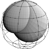
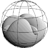
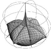
Figure 2. A peach front (Example 3.7) on the left, and a genus 1 complete front with 5 embedded ends in the middle (Example 4.6) with its caustic on the right.

Definition 3.5.

Let $f\colon{}\overline{M}^{2}\setminus\{p_{1},\dots,p_{n}\}\to H^{3}$ be a weakly complete flat front, and $(U,z)$ a complex coordinate of $\overline{M}^{2}$ with $z(p_{j})=0$. Suppose that all ends are regular, i.e. $G$ and $G_{*}$ have at most poles at $p_{1},\dots,p_{n}$, and that both $G$ and $G_{*}$ are non-constant. By a suitable motion in $H^{3}$, we may assume $G$ and $G_{*}$ have no poles at $p_{j}$. Then we have, with $m,m_{*}\in\boldsymbol{Z}_{+}$,

(3.6) $$G(z)=a+bz^{m}+o(z^{m})\quad\text{and}\quad G_{*}(z)=a_{*}+b_{*}z^{m_{*}}+o(z^{m_{*}}),$$

where $a,a_{*}\in\boldsymbol{C}$, $b,b_{*}\in\boldsymbol{C}\setminus\{0\}$ and $o(z^{m})$ and $o(z^{m_{*}})$ are higher order terms. We set

$$r_{p_{j}}(G)=m,\qquad r_{p_{j}}(G_{*})=m_{*}$$

to be the ramification numbers of $G$ and $G_{*}$ at $p_{j}$, respectively. Moreover, we define the multiplicity of $f$ at the end $p_{j}$ to be

$$m(f,p_{j})=\min\{m,m_{*}\}\quad\bigl{(}=\min\{r_{p_{j}}(G),r_{p_{j}}(G_{*})\}\bigr{)}\;.$$

If $f$ is complete at an end $p$, $m(f,p)=1$ if and only if the end $p$ is properly embedded [KUY2]. Roughly speaking, the multiplicity of a complete end is the winding number of a slice of the end (see [KRUY]). We have the following:

Proposition 3.6.

Let $f\colon{}\overline{M}^{2}\setminus\{p_{1},\dots,p_{n}\}\to H^{3}$ be a weakly complete flat front whose ends are all regular. If $Q$ has at most a simple pole at an end $p_{j}$, then $|\omega|^{2}$ and $|\theta|^{2}$ have finite orders at $p_{j}$ and the following identity holds:

(3.7) $$m(f,p_{j})=\min\left\{\bigl{|}1+\operatorname{ord}_{p_{j}}|\omega|^{2}\bigr{|},\bigl{|}1+\operatorname{ord}_{p_{j}}|\theta|^{2}\bigr{|}\right\}\;.$$

Proof.

Using a complex coordinate $z$ with $z(p_{j})=0$, assume $G$ and $G_{*}$ expand as in (3.6). As $Q$ has at most a simple pole at $p_{j}$, (2.17) and (2.20) give

$$s(\omega)=\frac{1}{z^{2}}\left(\frac{1-m^{2}}{2}+o(1)\right)\,dz^{2},\qquad s(\theta)=\frac{1}{z^{2}}\left(\frac{1-m_{*}^{2}}{2}+o(1)\right)\,dz^{2}.$$

So, by Section 2, $|\omega|^{2}$ and $|\theta|^{2}$ are of finite order (and well defined) at $p_{j}$. Thus $\omega$ and $\theta$ are of the form in (3.1), and

$$\mu=\operatorname{ord}_{p_{j}}|\omega|^{2}=\pm m-1,\qquad\mu_{*}=\operatorname{ord}_{p_{j}}|\theta|^{2}=\pm m_{*}-1.$$

Hence $m(f,p_{j})=\min\{m,m_{*}\}=\min\left\{|\mu+1|,|\mu_{*}+1|\right\}$ satisfies (3.7). ∎

Next, we give a weakly complete example that is neither complete nor of finite type.

Example 3.7 (The peach front in [KUY2]).

Let $b\in\boldsymbol{C}$ be a non-vanishing complex number. We define rational functions on $\boldsymbol{C}\cup\{\infty\}$ by

$$G=z,\qquad G_{*}=z-b.$$

By Fact 2.7, we get a holomorphic Legendrian curve

$$\mathcal{E}=\left(\begin{array}[]{rr}\dfrac{z}{c}\,e^{-z/b}&\dfrac{c}{b}(z-b)e^{z/b}\\[6.0pt] \dfrac{1}{c}\,e^{-z/b}&\dfrac{c}{b}e^{z/b}\end{array}\right)$$

with

$$\omega=-\frac{1}{c^{2}}e^{-2z/b}\,dz,\qquad\theta=\frac{c^{2}}{b^{2}}e^{2z/b}\,dz,\qquad ds^{2}_{1,1}=|\omega|^{2}+|\theta|^{2}\geq\frac{2}{|b|^{2}}|dz|^{2},$$

which implies that $f=\mathcal{E}\mathcal{E}^{*}$ is a weakly complete flat front in $H^{3}$, called a peach front. As the singular set of $f$ given by $|\theta|=|\omega|$ accumulates at $z=\infty$ for all $c$, $f$ and its parallel fronts are all not complete. By Theorem 3.4, $f$ is not of finite type. As we will see in Section 6, the peach fronts are characterized by the property that their caustics are horospheres. Figure 2 shows the peach front for $b=c=1$.

4. Examples

Let $M^{2}$ be a Riemann surface and $d\sigma^{2}$ a flat metric compatible to the conformal structure of $M^{2}$ (we call $d\sigma^{2}$ a “flat conformal metric”). Then there exists a developing map (as a holomorphic map)

$$\varphi\colon{}\widetilde{M}^{2}\longrightarrow\boldsymbol{R}^{2}=\boldsymbol{C}$$

such that $d\sigma^{2}$ is the pull-back of the canonical metric of $\boldsymbol{R}^{2}$, where $\pi\colon{}\widetilde{M}^{2}\to M^{2}$ is the universal cover of $M^{2}$. The differential $d\varphi$ is a holomorphic $1$-form on $\widetilde{M}^{2}$, and

(4.1) $$d\sigma^{2}=|d\varphi|^{2}.$$

Such a $1$-form $d\varphi$ is determined up to multiplication by a unit complex number. We call $d\varphi$ the associated $1$-form of the metric $d\sigma^{2}$.

For example, a flat front $f\colon{}M^{2}\to H^{3}$ without umbilics gives two flat conformal metrics $|\omega|^{2}$ and $|\theta|^{2}$ globally defined on $M^{2}$, with associated $1$-forms $\omega$ and $\theta$. (At an umbilic point $q$ of $f$, one of $\omega$ and $\theta$ will vanish, see (2.5). So one of the metrics $|\omega|^{2}$ or $|\theta|^{2}$ will degenerate at $q$.)

To construct examples, we introduce the following result.

Theorem 4.1.

Let $M^{2}$ be a Riemann surface and $|\omega|^{2}$ be a flat conformal metric on $M^{2}$ with associated $1$-form $\omega$. Let $G$ be a meromorphic function on $M^{2}$. Suppose that $d\sigma^{2}=|\omega|^{2}+|\theta|^{2}$ is a smooth and positive definite metric on $M^{2}$, where

(4.2) $$\theta=\frac{Q}{\omega},\qquad Q=\frac{s(\omega)-S(G)}{2}.$$

Then the map $f=\mathcal{E}\mathcal{E}^{*}:M^{2}\to H^{3}$ given by (2.12) gives a flat front with canonical forms $\omega$ and $\theta$, Hopf differential $Q$, and $G$ as one of its hyperbolic Gauss maps.

Theorem 4.1 follows directly from Fact 2.5 and (2.17). Moreover, we have:

Proposition 4.2.

In the situation of Theorem 4.1, suppose also that $M^{2}$ is biholomorphic to $\overline{M}^{2}\setminus\{p_{1},\dots,p_{n}\}$, for some compact Riemann surface $\overline{M}^{2}$. Then each end $p_{j}$ of $f$ is weakly complete if $p_{j}$ is a pole of $Q$ of order $2$.

Proof.

If $Q=\omega\theta$ has a pole of order $2$ at $p_{j}$, we have

$$\operatorname{ord}_{p_{j}}|\omega|^{2}+\operatorname{ord}_{p_{j}}|\theta|^{2}=-2.$$

Thus $\min\{\operatorname{ord}_{p_{j}}|\omega|^{2},\operatorname{ord}_{p_{j}}|\theta|^{2}\}\leq-1$ and $ds^{2}_{1,1}$ is complete. ∎

Here we construct higher genus flat fronts with regular ends, for which the ends might not be embedded. We begin with the following result, due to Troyanov:

Fact 4.3.

Let $\overline{M}^{2}$ be a compact Riemann surface with $p_{1},\dots,p_{n}\in{\overline{M}}^{2}$, and let $\mu_{1},\dots,\mu_{n}$ be real numbers which satisfy

$$\chi({\overline{M}}^{2})+\sum_{j=1}^{n}\mu_{j}=0.$$

Then there exists a flat conformal (positive definite) metric $d\sigma^{2}$ on $M^{2}=\overline{M}^{2}\setminus\{p_{1},\dots,p_{n}\}$ such that $\operatorname{ord}_{p_{j}}d\sigma^{2}=\mu_{j}$ for each $j=1,\dots,n$. Such a metric is unique up to homothety.

This fact is proved in [T] for $\mu_{j}>-1$, but the same argument works for any real numbers $\mu_{j}$. For the metric $d\sigma^{2}$ in Fact 4.3, the formal sum $\mu_{1}p_{1}+\dots+\mu_{n}p_{n}$ is called the singular divisor of $d\sigma^{2}$. With it, we can prove the following:

Theorem 4.4.

Given any compact Riemann surface $\overline{M}^{2}$ and meromorphic function $G$ on $\overline{M}^{2}$ with branch points $p_{1},\dots,p_{n}$, there exists a complete flat front $f\colon{}\overline{M}^{2}\setminus\{p_{1},\dots,p_{n}\}\to H^{3}$ with all ends $p_{j}$ regular and with hyperbolic Gauss map $G$.

Proof.

By a suitable motion in $H^{3}$, we may assume $G$ has no poles at $p_{1},\dots,p_{n}$. Let $m_{j}$ be the ramification number of $G$ at $p_{j}$ (see Definition 3.5). We can choose an $n$-tuple of real numbers $\mu_{1},\dots,\mu_{n}$ such that $\mu_{j}\neq\pm m_{j}-1$ $(j=1,\dots,n)$ and

$$\chi({\overline{M}}^{2})+\sum_{j=1}^{n}\mu_{j}=0\;.$$

By Fact 4.3, there exists a flat conformal metric $d\sigma^{2}$ on $M^{2}=\overline{M}^{2}\setminus\{p_{1},\dots,p_{n}\}$ with singular divisor $\mu_{1}p_{1}+\cdots+\mu_{n}p_{n}$. Then we can write $d\sigma^{2}=|\omega|^{2}$ where $\omega$ is a holomorphic $1$-form on $\widetilde{M}^{2}$, see (4.1). By Theorem 4.1 we can construct a flat front $f\colon{}\widetilde{M}^{2}\to H^{3}$ from the data $(G,\omega)$. Moreover, since $|\omega|$ is well-defined on $M^{2}$, any given deck transformation of $M^{2}$ changes $\omega$ to $e^{i\beta}\omega$ for some $\beta\in\boldsymbol{R}$. Hence $f$ is single-valued on $M^{2}$ by (2.12), that is, $f\colon{}M^{2}\to H^{3}$. Since $\mu_{j}\neq\pm m_{j}-1$, $Q$ has a pole of order $2$ at each $p_{j}$, by (2.17). Then by Proposition 4.2, $f$ is weakly complete at $p_{j}$. Then, since $\operatorname{ord}_{p_{j}}|\omega|^{2}$ and $\operatorname{ord}_{p_{j}}Q$ are finite, $\operatorname{ord}_{p_{j}}|\theta|^{2}$ is as well, so $f$ is of finite type. Then by Theorem 3.4, there exist infinitely many complete flat fronts in the parallel family of $f$, all with hyperbolic Gauss map $G$. Since $G$ has no essential singularity, each $p_{j}$ is a regular end (see Proposition 5.6 below). ∎

Remark 4.5.

Let $\overline{M}^{2}$ be a genus $k$ hyperelliptic Riemann surface with associated meromorphic function $G\colon{}\overline{M}^{2}\to\boldsymbol{C}\cup\{\infty\}$ of degree $2$ having branch points $p_{1},\dots,p_{n}$ ($n=2k+2$). Take a suitable integer $m$ and reals $\nu_{1},\dots,\nu_{m}<-1$ so that

$$\chi(\overline{M}^{2})+n+\sum_{j=1}^{m}\nu_{j}=0.$$

Choosing points $q_{1},\dots,q_{m}\in\overline{M}^{2}\setminus\{p_{1},\dots,p_{n}\}$, there exists a flat conformal metric $d\sigma^{2}=|\omega|^{2}$ whose divisor is

$$\sum_{j=1}^{m}\nu_{j}q_{j}+\sum_{l=1}^{n}p_{l}.$$

Then the flat front constructed from $(G,\omega)$ is well-defined on

$$M^{2}=\overline{M}^{2}\setminus\{p_{1},\dots,p_{n},q_{1},\dots,q_{m}\}.$$

Moreover, each $q_{j}$ is a regular end (see Proposition 5.6), and since $G$ does not branch at $q_{j}$, it is a properly embedded end (Proposition 3.12 of [KUY2]). Then, since $\operatorname{ord}_{p_{l}}|\omega|^{2}=1$ and $p_{l}$ is a branch point of $G$ with multiplicity $1$, (2.20), (2.22) and (2.17) yield that $Q$ has at most a simple pole at $p_{l}$. So we expect that generically $Q$ has a simple pole at each $p_{l}$. Hence $\operatorname{ord}_{p_{l}}|\theta|^{2}=-2$ and Proposition 3.6 gives $m(f,p_{l})=1$, implying that $p_{l}$ is an embedded end. Thus we can expect the existence of many higher genus flat fronts with embedded ends. If $m=1$, such an $f$ might have genus $k$ with $2k+3$ embedded ends (one end from $q_{1}$ and $2k+2$ ends from the $p_{l}$). In fact, when $k=1$ such an example is given explicitly in [KUY2]. So the next natural question is:

Problem.

Is there a complete flat front in $H^{3}$ of genus $k\geq 1$ with $2k+2$ embedded ends?

Even when $k=1$, no such examples are known; the problem was raised in [KUY2, Remark 3.17] for $k=1$. The following examples are related to this problem.

Example 4.6.

We construct flat fronts of genus $k\geq 1$ with $4k+1$ embedded ends, which are canonical generalizations of the $5$-ended genus $1$ fronts in [KUY2]. Choose a polynomial $\varphi(z)$ so that

1. $\varphi(z)=z^{2k}+a_{1}z^{k-1}+\dots+a_{k-1}z+a_{k}$, where $a_{1}\neq 0$, $a_{k}\neq 0$, and

2. $\varphi(z)$ has only simple roots, and

3. $(z\varphi(z))^{\prime}=\varphi(z)+z\varphi^{\prime}(z)$ also has only simple roots.

Consider the genus $k$ hyperelliptic Riemann surface defined by $w^{2}=z\varphi(z)$. Set

(4.3) $$G=w,\qquad G_{*}=\frac{h}{w},\quad\text{where}\quad h=h(z)=\frac{1}{2k+1}{\bigl{(}2kz\varphi(z)-z^{2}\varphi^{\prime}(z)\bigr{)}}.$$

Then we have

(4.4) $$\frac{dG}{G-G_{*}}=\frac{G\,dG}{G^{2}-G_{*}G}=\frac{\varphi(z)+z\varphi^{\prime}(z)}{2(z\varphi(z)-h(z))}=\frac{(2k+1)\,dz}{2z}.$$

Clearly $G$ is of degree $2k+1$. Since $h/w$ has only simple poles and only at the zeros of $\varphi(z)$, $G_{*}$ has degree $2k$. Thus $\deg G+\deg G_{*}=4k+1$. By (4.4),

(4.5) $$\xi=\exp\int\frac{dG}{G-G_{*}}=z^{(2k+1)/2}$$

has only purely imaginary monodromy. Moreover, (4.3) implies

(4.6) $$G-G_{*}=\frac{1}{w}(w^{2}-h)=\frac{z}{(2k+1)w}(\varphi+z\varphi^{\prime}).$$

So applying Fact 2.7, we get a flat front

$$f\colon M^{2}=\overline{M}^{2}\setminus\{(z,w)\,;\,z\bigl{(}\varphi(z)+z\varphi^{\prime}(z)\bigr{)}=0\}\longrightarrow H^{3}.$$

By (4.6), $f$ has exactly $4k+1$ ends, since the ends are the zeros of $z\bigl{(}\varphi(z)+z\varphi^{\prime}(z)\bigr{)}$. Note that $z=\infty$ is not an end, since $G(\infty)=\infty$ and $G_{*}(\infty)=0$. By (4.5) and (2.15), one canonical $1$-form is $\omega=-z^{-(2k+1)}dG$, and $f$ could have been made using Fact 2.5 as well, with this $\omega$. As

$$dG_{*}=\frac{h^{\prime}w-hw^{\prime}}{w^{2}}dz=\frac{h^{\prime}w^{2}-hww^{\prime}}{w^{3}}dz=\frac{h^{\prime}z\varphi-{h}(z\varphi)^{\prime}/2}{w^{3}}dz,$$

we have by (4.6), (4.4) and (2.15) that

$$Q=-\frac{2k+1}{2z}\cdot\frac{zh^{\prime}\varphi-{h}(z\varphi)^{\prime}/2}{w^{2}(w^{2}-h)}dz^{2}=-\frac{(2k+1)^{2}}{2}\cdot\frac{{h^{\prime}\varphi}-{(h/z)}(z\varphi)^{\prime}/2}{zw^{2}\left(\varphi+z\varphi^{\prime}\right)}dz^{2}.$$

Here, $dz/w$ has no poles and zeros at the zeros of $w$. Since $a_{k}\neq 0$, the origin $z=0$ is a pole of order $2$ of $Q$, and thus it is a weakly complete end, by Proposition 4.2. On the other hand, $Q$ has simple poles at the other ends. However, $\omega$ has zeros at the ends other than $z=0$, by (4.4). Hence the orders of $|\theta|^{2}$ are less than $-1$ at such ends, and then they are weakly complete. Any branch point of $G$ in $\overline{M}^{2}$ must be a zero of $(z\varphi)^{\prime}$, and thus must be an end of $f$, so $G$ has no branch points on $M^{2}\setminus\{z=\infty\}$. Moreover $a_{1}a_{k}\neq 0$ implies that $G_{*}$ does not branch at $z=\infty$ and $z=0$. Thus $f$ has no branch points anywhere on $M^{2}$, by Theorem 2.9 of [KUY2]. Since $f$ is weakly complete and of finite type, there exist infinitely many complete fronts in the parallel family of $f$, by Theorem 3.4. By equality of the Osserman-type inequality ([KUY2, Theorem 3.13]), all the ends of $f$ are properly embedded.

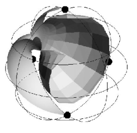
Figure 3. A genus $2$ flat front with $10$ embedded ends, coming from a variant of the approach in Example 4.6. It is defined on the closed Riemann surface $\overline{M}^{2}=\{(z,w)\in(\boldsymbol{C}\cup\{\infty\})^{2}\,;\,w^{2}=z(z^{2}-1)(z^{2}-9/4)\}$ with $10$ points removed, and with data $G=w$ and $G_{*}=(5w-2z(dw/dz))/5$. Because $G$ and $G_{*}$ have no common branch points, the surface is a front with embedded ends. The portion shown here is the image of one sheet in $\overline{M}^{2}$ over the quadrant $\{z\in\boldsymbol{C}\cup\{\infty\}\,;\,\operatorname{Re}z\geq 0,\operatorname{Im}z\geq 0\}$ in the $z$-plane, and is one-eighth of the full surface. The planar boundary curves of this portion lie in planes of reflective symmetry of the full surface. The four ends appearing in the boundary of this portion are marked with black dots.

Finally, we shall show that $\varphi(z)=z^{2k}-2cz^{k-1}-1$ satisfies the above conditions (b), (c) for a suitable $c\in\boldsymbol{R}$. When $k=1$ and $c=0$, $f$ is just the example in [KUY2, Example 4.6]. When $k\geq 2$, we set $c=k/(k-1)$. Then

$$\varphi^{\prime}(z)=2kz^{k-2}\bigl{(}z^{k+1}-1\bigr{)}.$$

Let $p\neq 0$ be a zero of $\varphi^{\prime}(z)$, so $p^{k+1}=1$ and $p^{2}\varphi(p)=1-p^{2}-2k/(k-1)$. If $\varphi(p)=0$, then $p^{2}=(1+k)/(1-k)$ and $|p|\neq 1$. So $\varphi(z)$ has no double roots. Now

$$(z\varphi)^{\prime\prime}=2kz^{k-2}((2k+1)z^{k+1}-k).$$

Let $q\neq 0$ be a zero of $(z\varphi)^{\prime\prime}$. Then we have $q^{k+1}=k/(2k+1)$. Hence $|q|^{2}=\bigl{(}k/(2k+1)\bigr{)}^{2/(k+1)}$ is not a rational number. On the other hand,

$$q^{2}(z\varphi)^{\prime}|_{z=q}=(2k+1)\left(\frac{k}{2k+1}\right)^{2}-\frac{2k^{2}}{k-1}\cdot\frac{k}{2k+1}-q^{2}.$$

If $(z\varphi)^{\prime}|_{z=q}=0$, we have $q^{2}=k^{2}(1+k)/((2k+1)(1-k))\in\boldsymbol{Q}$, a contradiction. Thus both $\varphi$ and $(z\varphi)^{\prime}$ have only simple roots, and $\varphi(z)$ satisfies conditions (b), (c).

5. p-fronts

Now we consider flat p-fronts, starting with a proof of Theorem B.

Theorem B.

Let $f\colon M^{2}\to H^{3}$ be a flat p-front, then $M^{2}$ is orientable.

As noted in the introduction, the other space forms $\boldsymbol{R}^{3}$ and $S^{3}$ admit flat Möbius bands (see Gálvez and Mira [GM1]). So Theorem B is special to $H^{3}$. Kitagawa [Ki] proved the orientability of compact flat surfaces in $S^{3}$.

Proof of Theorem B.

As $f$ is a p-front, for any $p\in M^{2}$ there exists a neighborhood $U_{p}\subset M^{2}$ of $p$ such that $f|_{U_{p}}$ is a front. We may assume that $U_{p}$ is simply connected. Then as noted in Section 2, there exists a unique complex structure on $U_{p}$ such that both hyperbolic Gauss maps $G$ and $G_{*}$ are meromorphic.

Since $f|_{U_{p}}$ is a front, at least one of $G$ or $G_{*}$ is not branched at $p$, by Theorem 2.9 of [KUY2]. Without loss of generality, we may assume $G$ and $G_{*}$ are finite at $p$. Choosing $U_{p}$ sufficiently small, we have a local complex coordinate $z=G|_{U_{p}}$ or $z=G_{*}|_{U_{p}}$ on $U_{p}$ at each point $p\in M^{2}$. Since $G\circ G^{-1}$ and $G_{*}\circ G^{-1}_{*}$ are identity maps and either $G\circ G^{-1}_{*}$ or $G_{*}\circ G^{-1}$ is well-defined and holomorphic on $U_{p}$ for each $p\in M^{2}$, the transition function on $U_{p}\cap U_{q}$ for two distinct points $p$ and $q$ is always holomorphic. So we can extend this local complex structure on $U_{p}$ to all of $M^{2}$. ∎

When we consider a flat p-front, we always regard $M^{2}$ as a Riemann surface with the complex structure given in the proof of Theorem B. Note that co-orientability is defined in the introduction.

Theorem 5.1.

Let $f\colon M^{2}\to H^{3}$ be a non-co-orientable flat p-front with universal cover $\pi\colon{}\widetilde{M}^{2}\to M^{2}$. Then there exists a Legendrian immersion

$$\mathcal{E}_{f}:\widetilde{M}^{2}\longrightarrow\operatorname{SL}(2,\boldsymbol{C})$$

and a covering transformation $\tau\colon{}\widetilde{M}^{2}\to\widetilde{M}^{2}$ such that

$$\mathcal{E}_{f}\circ\tau=\mathcal{E}_{f}\begin{pmatrix}0&i\,\\ i\,&0\end{pmatrix}\,(=\mathcal{E}^{\natural}_{f}).$$

We call this $\mathcal{E}_{f}$ the adjusted lift of the p-front $f$. Conversely, if a lift $\mathcal{E}_{f}$ satisfies $\mathcal{E}_{f}\circ\tau=\mathcal{E}^{\natural}_{f}$ for some covering transformation $\tau$, $f=\mathcal{E}_{f}\mathcal{E}_{f}^{*}=\mathcal{E}^{\natural}_{f}(\mathcal{E}^{\natural}_{f})^{*}$ is non-co-orientable.

Proof of Theorem 5.1.

Take a holomorphic Legendrian lift $\mathcal{E}_{0}\colon{}\widetilde{M}^{2}\to\operatorname{SL}(2,\boldsymbol{C})$ of $f$; it is determined up to right-multiplication by a matrix in $\operatorname{SU}(2)$. We now change $\mathcal{E}_{0}$ to an adjusted lift. The flat front $\tilde{f}=\mathcal{E}_{0}\mathcal{E}_{0}^{*}\colon{}\widetilde{M}^{2}\to H^{3}$ satisfies $f\circ\pi=\tilde{f}$. The unit normal vector of $\tilde{f}$ is $\tilde{\nu}=\mathcal{E}_{0}e_{3}\mathcal{E}_{0}^{*}$, by (2.3). If $p_{1},p_{2}\in\pi^{-1}(p)$, then $\tilde{\nu}(p_{1})=\pm\tilde{\nu}(p_{2})$. So there exists a (unique) representation $\delta\colon{}\pi_{1}(M^{2})\to\{\pm 1\}$ such that

$$\tilde{\nu}\circ T=\delta(T)\tilde{\nu}\qquad(T\in\pi_{1}(M^{2})),$$

where the fundamental group $\pi_{1}(M^{2})$ is identified with the covering transformation group. Since $f$ is non-co-orientable, $\delta$ is surjective. Letting $\check{M}^{2}=\widetilde{M}^{2}/\operatorname{Ker}\delta$ with associated nontrivial covering involution $\sigma$ on $\check{M}^{2}$, $\check{\nu}=\mathcal{E}_{0}e_{3}\mathcal{E}_{0}^{*}$ is single-valued on $\check{M}^{2}$, so $\check{f}=\mathcal{E}_{0}\mathcal{E}_{0}^{*}\colon{}\check{M}^{2}\to H^{3}$ is a flat front because its unit normal vector $\check{\nu}$ is well-defined, and $\check{\nu}\circ\sigma=-\check{\nu}$. Since $\widetilde{M}^{2}$ is universal, there exists a lift $\tau\colon\widetilde{M}^{2}\to\widetilde{M}^{2}$ of $\sigma$. As $\tau$ is holomorphic and $\mathcal{E}_{0}\mathcal{E}^{*}_{0}=(\mathcal{E}_{0}\circ\tau)(\mathcal{E}_{0}\circ\tau)^{*}$, there exists an $\operatorname{SU}(2)$-matrix

$$R=\begin{pmatrix}p&-\bar{q}\\ q&\hphantom{-}\bar{p}\end{pmatrix}\qquad(|p|^{2}+|q|^{2}=1)$$

such that $\mathcal{E}_{0}\circ\tau=\mathcal{E}_{0}R$. Since $\check{\nu}\circ\sigma=-\check{\nu}$, we have $\mathcal{E}_{0}e_{3}\mathcal{E}_{0}^{*}=-\mathcal{E}_{0}Re_{3}R^{*}\mathcal{E}_{0}^{*}$, so $Re_{3}R^{*}=-e_{3}$, implying $p=0$. Thus

$$\mathcal{E}_{f}=\mathcal{E}_{0}a,\qquad\text{where}\quad a=\begin{pmatrix}\sqrt{i/q}&0\\ 0&\overline{\sqrt{i/q}}\end{pmatrix},$$

satisfies $f=\mathcal{E}_{f}\mathcal{E}^{*}_{f}$ and $\mathcal{E}_{f}\circ\tau=\mathcal{E}^{\natural}_{f}$. ∎

Corollary 5.2.

Let $f\colon M^{2}\to H^{3}$ be a non-co-orientable flat p-front. Then there is a double cover $\check{\pi}\colon\check{M}^{2}\to M^{2}$ such that $\check{f}=f\circ\check{\pi}\colon\check{M}^{2}\to H^{3}$ is a front. Moreover, there exists a covering transformation $\tau\colon\check{M}^{2}\to\check{M}^{2}$ with $\check{f}\circ\tau=\check{f}$ satisfying

$$\check{G}\circ\tau=\check{G}_{*},\quad\check{G}_{*}\circ\tau=\check{G},\quad\check{\omega}\circ\tau=\check{\theta},\quad\check{\theta}\circ\tau=\check{\omega}\quad\text{and}\quad\check{Q}\circ\tau=\check{Q},$$

where $\check{G}=G\circ{\check{\pi}}$ and $\check{G}_{*}$, $\check{\omega}$, $\check{\theta}$, $\check{Q}$ are defined similarly.

Thus, for a p-front, the Hopf differential $Q$ and $ds^{2}_{1,1}=|\omega|^{2}+|\theta|^{2}$ are well-defined.

Definition 5.3.

A non-co-orientable flat p-front $f$ is called complete (resp. weakly complete, finite type) if its double cover $\check{f}$ as in Corollary 5.2 is complete (resp. weakly complete, finite type).

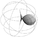
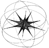
Figure 4. The p-front in Example 3.7 that is not globally a caustic on the left, and the caustic with dihedral cross $\boldsymbol{Z}^{2}$ symmetry for the fronts produced by $G=z^{3}$ and $G_{*}=z^{-5}$ and $M^{2}=\boldsymbol{C}\setminus\{z\,;\,z^{8}=1\}$ on the right.

Proposition 5.4.

Let $f\colon{}M^{2}\to H^{3}$ be a flat p-front. The following hold:

1. If $f$ is complete, then it is weakly complete and of finite type.

2. If $f$ is weakly complete and of finite type, there exists a compact Riemann surface $\overline{M}^{2}$ such that $M^{2}$ is biholomorphic to $\overline{M}^{2}\setminus\{p_{1},\dots,p_{n}\}$, for finitely many distinct points $p_{1},\dots,p_{n}$ in $\overline{M}^{2}$. Moreover, $ds^{2}_{1,1}$ has finite order at $p_{1},\dots,p_{n}$ and $Q$ extends to a meromorphic $2$-differential on $\overline{M}^{2}$.

Proof.

(1) follows immediately from Proposition 3.1. To show (2), $M^{2}$ is biholomorphic to $\overline{M}^{2}\setminus\{p_{1},\dots,p_{n}\}$ by Huber’s theorem, just as in the proof of Proposition 3.2. We will call the points $\{p_{1},\dots,p_{n}\}$ the ends of $f$ (Definition 5.5). Suppose an end $p_{j}$ is co-orientable, that is, the restriction of $f$ to a sufficiently small punctured neighborhood of $p_{j}$ is co-orientable (see Definition 5.8). Then Proposition 3.2 implies $\omega$, $\theta$ have finite order at $p_{j}$, and $Q$ is meromorphic there. If $p_{j}$ is not co-orientable, we take a punctured neighborhood $U_{j}^{*}$ of $p_{j}$, and let $\check{U}_{j}^{*}$ be its double cover. Lifting $f|_{U_{j}^{*}}$ to $\check{f}:\check{U}_{j}^{*}\to H^{3}$, $\check{f}$ is now a weakly complete co-orientable end of finite type. Its canonical $1$-forms $\check{\omega}$, $\check{\theta}$ are of finite order, and $d\check{s}^{2}_{1,1}=|\check{\omega}|^{2}+|\check{\theta}|^{2}$ is complete and of finite order, and its Hopf differential $\check{Q}$ extends meromorphically across the puncture of $\check{U}_{j}^{*}$, by Proposition 3.2. Noting that $d\check{s}^{2}_{1,1}$ is actually well defined on $U_{j}^{*}$ and equals $ds^{2}_{1,1}$ there, and that $\check{Q}$ projects to the Hopf differential of $f|_{U_{j}^{*}}$ on $U_{j}^{*}$, the proof is completed. ∎

To observe the behavior of ends of $p$-fronts, we review properties of regular ends of fronts:

Definition 5.5.

A p-front $f\colon{}M^{2}\to H^{3}$ is said to be of finite topology if there exists a compact Riemann surface $\overline{M}^{2}$ such that $M^{2}$ is homeomorphic to $\overline{M}^{2}\setminus\{p_{1},\dots,p_{n}\}$. Such points $p_{1},\dots,p_{n}$ are called the ends of $f$.

An end of a weakly complete flat p-front of finite topology is said to be of puncture-type if it is biholomorphic to a punctured disk, and to be annular if it is biholomorphic to an annulus $\{z\,;\,r_{1}<|z|<r_{2}\}$, $0<r_{1}<r_{2}<\infty$.

A puncture-type end $p$ of a weakly complete flat front is said to be regular if both $G$, $G_{*}$ have at most poles at $p$, and to be irregular otherwise.

For a weakly complete flat p-front, a puncture-type end $p$ is said to be regular if the corresponding end $\check{p}$ of $\check{f}$ is regular, and to be irregular otherwise.

Proposition 5.6.

For an end $p$ of a flat front of finite type, the following conditions are equivalent:

1. The end $p$ is regular.

2. One of $G$, $G_{*}$ has at most a pole at $p$.

3. The Hopf differential $Q$ has at most a pole of order $2$ at $p$.

Proof.

This was proven in [GMM, Theorem 4] for complete ends. Reading that proof carefully, one sees that it applies to flat fronts of finite type as well. ∎

Proposition 5.7.

Let $f\colon M^{2}=\overline{M}^{2}\setminus\{p_{1},\dots,p_{n}\}\to H^{3}$ be a weakly complete flat front whose ends are all regular. Then $f$ is of finite type if and only if the Hopf differential has at most a pole of order $2$ at each end.

Proof.

One direction follows from Proposition 5.6, so we prove the other direction here. Choose an end $p_{j}$. By (2.22), $\omega$ and $\theta$ have finite order at $p_{j}$ if and only if $s(\omega)$ and $s(\theta)$ have at most poles of order $2$. Since $G$, $G_{*}$ are meromorphic at $p_{j}$, $S(G)$ and $S(G_{*})$ have at most poles of order $2$. Then (2.17) implies that $\operatorname{ord}_{p_{j}}Q\geq-2$ if and only if $s(\omega)$ and $s(\theta)$ have at most poles of order $2$. ∎

Definition 5.8.

For a weakly complete flat p-front $f\colon{}\overline{M}^{2}\setminus\{p_{1},\dots,p_{n}\}\to H^{3}$, an end $p_{j}$ is called co-orientable if the restriction of $f$ to a sufficiently small punctured neighborhood of $p_{j}$ is co-orientable, and is otherwise called non-co-orientable.

A co-orientable regular end $p$ of a flat p-front $f$ can be considered as a regular end of a flat front, and we have already defined its multiplicity $m(f,p)$ (Definition 3.5). We also now define the multiplicity of a non-co-orientable end. Let

$$f\colon{}D^{*}(\varepsilon)=\{z\,;\,0<|z|<\varepsilon\}\longrightarrow H^{3}$$

be a non-co-orientable end at $p$. Then there exists a lift (as a p-front) $\check{f}\colon{}\check{D}^{*}(\varepsilon)\to H^{3}$ of $f$, where $\check{D}^{*}(\varepsilon)$ is the double covering of $D^{*}(\varepsilon)$. We set

(5.1) $$m(f,p)=m(\check{f},\check{p})/2$$

and call it the multiplicity of the end $p$ of $f$. Thus we have defined the multiplicity of any regular end of a weakly complete p-front, taking its value in $\frac{1}{2}\boldsymbol{Z}$. Let $f\colon{}M^{2}\to H^{3}$ be a weakly complete flat front with regular ends. If $f$ is co-orientable, the hyperbolic Gauss maps $G$, $G_{*}$ of $f$ are single-valued on $M^{2}$ and we set

$$\deg\mathcal{G}_{f}=\deg G+\deg G_{*},$$

which we call the total degree of the Gauss maps of $f$. When $f$ is non-co-orientable, there exists a lift $\check{f}\colon{}\check{M}^{2}\to H^{3}$ of $f$, where $\check{M}^{2}$ double covers $M^{2}$, and we set

$$\deg\mathcal{G}_{f}=(\deg\mathcal{G}_{\check{f}})/2\;.$$

It follows from [KUY2, Theorem 3.13] that

(5.2) $$\deg{\mathcal{G}}_{f}\geq\#\{\text{\rm non-co-orientable ends}\}/2+\#\{\text{\rm co-orientable ends}\}$$

for a weakly complete flat p-front of finite type whose ends are all regular. When $f$ is complete, equality implies all ends are properly embedded. We note that complete ends are automatically co-orientable: Suppose a complete end $p$ of a p-front $f\colon{}M^{2}\to H^{3}$ is non-co-orientable. Take the double cover $\check{M}^{2}$, the lift $\check{f}\colon{}\check{M}^{2}\to H^{3}$ and a complex coordinate $z$ of $\check{M}^{2}$ around the (unique) lift $\check{p}$ of $p\in\overline{M}^{2}$ with $z(\check{p})=0$. Since $\check{p}$ is also a complete end, $\check{f}$ is of finite type and the canonical forms are written as

$$\check{\omega}=cz^{\mu}\bigl{(}1+o(1)\bigr{)}\,dz\qquad\text{and}\qquad\check{\theta}=c_{*}z^{\mu_{*}}\bigl{(}1+o(1)\bigr{)}\,dz,$$

where $c,c_{*}$ are non-zero constants and $\mu,\mu_{*}\in\boldsymbol{R}$. Here, by Corollary 5.2, we have $|c|=|c_{*}|$ and $\mu=\mu_{*}$. Hence we have $|\check{\rho}|=|\check{\theta}/\check{\omega}|=1+o(1)$, which implies that the singular set of $\check{f}$ accumulates at $\check{p}$, contradicting that $\check{p}$ is a complete end.

Example 5.9 (Weakly complete p-fronts with $3$ ends).

This example is of interest, because it is neither a front nor globally a caustic (see Remark 6.8). Set

$$G=\frac{z^{2}+\tfrac{z}{b}}{z+b}\quad\text{and}\quad G_{*}=\frac{z^{2}-\tfrac{z}{b}}{b-z}\qquad(b\in\boldsymbol{R}\setminus\{0,\pm 1\})$$

which are defined on the Riemann surface $\check{M}^{2}=\boldsymbol{C}\setminus\{0,\pm 1\}$. Then Fact 2.7 gives a flat front $\check{f}_{b}\colon{}\check{M}^{2}\to H^{3}$ with hyperbolic Gauss maps $G$ and $G_{*}$. We also have

$$\xi =c\cdot\exp\int\frac{dG}{G-G_{*}}=c\frac{\sqrt{z}}{z+b}(z-1)^{(1-b)/2}(z+1)^{(1+b)/2},$$

$$\omega =-c^{-2}(z^{2}+2bz+1)z^{-1}(z-1)^{b-1}(z+1)^{-b-1}\,dz,$$

$$\theta =-c^{2}(z^{2}-2bz+1)z^{-1}(z-1)^{-b-1}(z+1)^{b-1}\,dz/4.$$

Now we set $c=\sqrt{2}$. Then $\omega\circ\tau=\theta$ holds, where $\tau\colon{}\check{M}^{2}\ni z\mapsto-z\in\check{M}^{2}$. Then $\mathcal{E}_{f_{b}}\circ\tau=\mathcal{E}^{\natural}_{f_{b}}$, and hence we have a well-defined flat p-front

$$f_{b}\colon{}M^{2}=(\check{M}^{2}/\sim)\longrightarrow H^{3}$$

where $z_{1}\sim z_{2}$ if and only if $z_{2}=\pm z_{1}$. The three ends of $f_{b}$ are at $z=0$ and $z=\infty$ and $z=\pm 1$. The ends at $z=0$, $z=\infty$ are non-co-orientable, and the end at $z=\pm 1$ is co-orientable. $f_{b}$ satisfies equality in (5.2).

6. Caustics

Roitman [R] showed that the caustic $C_{f}$ (or focal surface) of a flat surface $f$ is also flat, and gave a representation for $C_{f}$ in terms of $f$. In [KRSUY, Section 5], Roitman’s representation is described in the terminology below: Let $f\colon M^{2}\to H^{3}$ be a flat front with hyperbolic Gauss maps $G,G_{*}$. Let $q_{1},\dots,q_{m}\in M^{2}$ be the umbilic points of $f$. Then we can choose a single-valued square root

$$\beta=\sqrt{dG/dG_{*}}$$

defined on the universal cover $\widetilde{M}_{\mathrm{c}}$ of $M_{\mathrm{c}}=M^{2}\setminus\{q_{1},\dots,q_{m}\}$. The caustic $C_{f}$ is

$$C_{f}=\mathcal{E}_{\mathrm{c}}{\mathcal{E}_{\mathrm{c}}}^{*}\colon M_{\mathrm{c}}\longrightarrow H^{3}\;,$$

(6.1) $$\mathcal{E}_{\mathrm{c}}=\frac{\sqrt{i}}{\sqrt{2\beta(G-G_{*})}}\begin{pmatrix}G+\beta G_{*}&i\,(G-\beta G_{*})\\ 1+\beta&i\,(1-\beta)\end{pmatrix}\begin{pmatrix}\sqrt{i}&0\\ 0&1/\sqrt{i}\end{pmatrix}\in\operatorname{PSL}(2,\boldsymbol{C})\;,$$

where $\sqrt{i}=e^{\pi i/4}$. Note that $\mathcal{E}_{\mathrm{c}}\in\operatorname{PSL}(2,\boldsymbol{C})$ because of the sign ambiguity of $\sqrt{2\beta(G-G_{*})}$. The $\operatorname{SU}(2)$-matrix $\operatorname{diag}(\sqrt{i},1/\sqrt{i})$ in Equation (6.1) is not essential, and is included only so that $\mathcal{E}_{\mathrm{c}}$ changes to $\mathcal{E}_{\mathrm{c}}^{\natural}$ when $\beta$ changes to $-\beta$, i.e. so that $\mathcal{E}_{\mathrm{c}}$ becomes an adjusted lift. The hyperbolic Gauss maps ${G_{\mathrm{c}}},{G_{\mathrm{c}}}_{*}$ and the canonical forms ${\omega_{\mathrm{c}}}$, ${\theta_{\mathrm{c}}}$ of the caustic $C_{f}$ are

(6.2) $$({G_{\mathrm{c}}},{G_{\mathrm{c}}}_{*})=\left(\frac{G+\beta G_{*}}{1+\beta},\frac{G-\beta G_{*}}{1-\beta}\right),$$

(6.3) $${\omega_{\mathrm{c}}} =\frac{1}{4}\left\{\frac{2(\beta+1)^{2}}{G-G_{*}}dG_{*}-d\log\left(\frac{dG}{dG_{*}}\right)\right\},$$

(6.4) $${\theta_{\mathrm{c}}} =\frac{1}{4}\left\{\frac{2(\beta-1)^{2}}{G-G_{*}}dG_{*}-d\log\left(\frac{dG}{dG_{*}}\right)\right\}.$$

These two forms can be also expressed using $Q(=\omega\theta)$, $\rho(=\theta/\omega)$ of the original front $f$, as can the Hopf differential ${Q_{\mathrm{c}}}={\omega_{\mathrm{c}}}{\theta_{\mathrm{c}}}$ of $C_{f}$:

(6.5) $${\omega_{\mathrm{c}}}=i\sqrt{Q}+\frac{1}{4}d\log\rho,\quad{\theta_{\mathrm{c}}}=-i\sqrt{Q}+\frac{1}{4}d\log\rho,\quad{Q_{\mathrm{c}}}=Q+\left(\frac{d\log\rho}{4}\right)^{2},$$

where the sign of $\sqrt{Q}$ is chosen so that (6.5) is compatible with (6.3) and (6.4).

Proposition 6.1.

The caustic of a flat front is a p-front.

Proof.

By Theorem 2.9 of [KUY2], it suffices to prove that ${\omega_{\mathrm{c}}}$ and ${\theta_{\mathrm{c}}}$ have no common zeros. Let $p$ be an arbitrary point on the caustic. Since $p$ is not an umbilic point on the original front, i.e., $Q(p)\neq 0$, it follows from (6.5) that at least one of ${\omega_{\mathrm{c}}}(p),{\theta_{\mathrm{c}}}(p)$ is not zero. ∎

Example 6.2 (Caustics of rotational flat fronts).

Since the horosphere is totally umbilic, it has no caustic. For other rotational examples:

1. the caustic of a hyperbolic cylinder is a hyperbolic line,

2. the caustic of an hourglass is also a hyperbolic line,

3. the caustic of a snowman is a hyperbolic cylinder,

where hourglasses and snowmen are fronts of revolution with single conical singularities and cuspidal edge singularities, respectively (see [KUY2, Example 4.1]). In fact, snowmen are characterized by their caustics, as Proposition 6.3 shows:

Proposition 6.3.

Let $f$ be a flat front with caustic ${C_{f}}$. Then $f$ is locally a snowman if and only if ${C_{f}}$ is an open submanifold of a hyperbolic cylinder.

Proof.

As seen in Example 6.2, a flat front of revolution has a hyperbolic cylinder as its caustic if and only if it has a nonempty cuspidal edge set, so we need only show that if ${C_{f}}$ is a hyperbolic cylinder, then $f$ is a surface of revolution.

Assume ${C_{f}}\colon{}M^{2}\to H^{3}$ is a hyperbolic cylinder, so we may assume $M^{2}$ is an open subset of $\boldsymbol{C}\setminus\{0\}$ and

$${\theta_{\mathrm{c}}}=\frac{c^{2}}{4z}\,dz,\qquad{\omega_{\mathrm{c}}}=\frac{1}{c^{2}z}\,dz,$$

where $c\in\boldsymbol{R}\setminus\{0\}$ (see [KUY2, Example 4.1]). Then by (6.5), the Hopf differential $Q$ of $f$ is

$$Q=-\frac{1}{4}({\theta_{\mathrm{c}}}-{\omega_{\mathrm{c}}})^{2}=-\frac{a^{2}}{4}\frac{dz^{2}}{z^{2}}\qquad\left(a=\frac{c^{2}}{4}-\frac{1}{c^{2}}\right),$$

and the function $\rho$ satisfies

$$d\log\rho=\frac{2b}{z}\,dz,\qquad\text{and then}\qquad\rho=-kz^{2b}\qquad\left(b=\frac{1}{c^{2}}+\frac{c^{2}}{4}\right),$$

where $k\neq 0$ is a constant. Thus, we compute $\theta=\sqrt{Q\rho}$ and $\omega=Q/\theta$ as

$$\theta=\frac{\sqrt{k}}{2}az^{b-1}\,dz,\qquad\omega=\frac{1}{2\sqrt{k}}az^{-b-1}\,dz.$$

Hence $f$ is a part of a surface of revolution. ∎

One can check that the caustic of a peach front (Example 3.7) is a horosphere [R]. Peach fronts are also characterized by their caustics:

Proposition 6.4.

A flat front is locally a peach front if and only if its caustic is totally umbilic, i.e., is locally an open submanifold of a horosphere. In particular, a peach front is the only flat front whose caustic is the horosphere.

Proof.

Assume the caustic is totally umbilic, that is, ${Q_{\mathrm{c}}}=0$. Taking the dual lift if necessary, we may assume ${G_{\mathrm{c}}}$ is constant, and then applying a rigid motion of $H^{3}$ if necessary, we may assume ${G_{\mathrm{c}}}=0$. It follows from (6.2) that $G^{2}/G_{*}^{2}=dG/dG_{*}$, so $1/G_{*}-1/G$ is a constant. By a suitable motion of $H^{3}$, we can change $G$ and $G_{*}$ to $1/G_{*}$ and $1/G$, and then $G_{*}=G+\text{constant}$. If $G$ branches, then $G_{*}$ also branches, so the flat surface $f$ produced by $G$ and $G_{*}$ would not be a front, by Theorem 2.9 of [KUY2]. Hence we may assume $G=z$ is a coordinate for the front $f$, proving the assertion. ∎

Remark 6.5.

Propositions 6.3 and 6.4 show that if the caustic ${C_{f}}$ is complete without singularities (so is a cylinder or horosphere, see [GMM, Theorem 3]), then the original front $f$ must be a snowman or peach front.

Theorem 6.6.

Any flat p-front is locally the caustic of some flat front.

Proof.

For $f\colon M^{2}\to H^{3}$ a flat p-front, take any $p\in M^{2}$. Take a simply connected neighborhood $U$ of $p$, so the canonical forms ${\omega_{\mathrm{c}}}$, ${\theta_{\mathrm{c}}}$ of $f$ are single-valued on $U$. Set

$$Q_{s}=-\tfrac{1}{4}(e^{i\,s}{\omega_{\mathrm{c}}}-e^{-i\,s}{\theta_{\mathrm{c}}})^{2}\qquad(s\in\boldsymbol{R}).$$

Then $Q_{s}$ is a well-defined holomorphic $2$-differential on $U$. If $Q_{s}(p)=0$ for all $s$, then $\omega(p)=\theta(p)=0$, a contradiction, so we can choose a real number $s_{0}$ so that $Q_{s_{0}}(p)\neq 0$. Determine $\omega$ and $\theta$ by

$$\omega\theta=Q_{s_{0}},\quad\frac{\theta}{\omega}=\rho,\quad\text{where}\quad\rho=\rho(z)=\exp\left(\int_{z_{0}}^{z}2(e^{i\,s_{0}}{\omega_{\mathrm{c}}}+e^{-i\,s_{0}}{\theta_{\mathrm{c}}})\right)(\neq 0).$$

These $\omega$, $\theta$ yield a flat front $F=\mathcal{E}\mathcal{E}^{*}$ by solving (2.4), and the caustic of $F$ is $f$, up to a rigid motion of $H^{3}$. ∎

Remark 6.7.

The above proof implies that for a given p-front $f$, there is locally a two parameter family of fronts $F_{t,s}$ whose caustics are $f$. One of these parameters is the signed-distance $t$ of parallel fronts and the other is the $s$ in the proof above.

Remark 6.8.

The “locally” condition is necessary in Theorem 6.6, as there are flat p-fronts that are not caustics globally. In fact, the $f_{b}\colon M^{2}\to H^{3}$ defined in Example 5.9 is not a caustic over $M^{2}$ if $b\not\in\frac{1}{2}\boldsymbol{Z}$: Suppose, by way of contradiction, that $f_{b}$ is a caustic of some $f_{\mathrm{orig}}\colon M^{\prime}\to H^{3}$. By (6.5), we have

$$4\sqrt{Q_{\mathrm{orig}}}=i\Bigl{(}\frac{z-1}{z+1}\Bigr{)}^{b}\left\{\frac{z^{2}+2bz+1}{z(z^{2}-1)}-\frac{z^{2}-2bz+1}{z(z^{2}-1)}\Bigl{(}\frac{z+1}{z-1}\Bigr{)}^{2b}\right\}dz.$$

It follows that $Q_{\mathrm{orig}}$ is not well-defined at $z=0$ if $b\not\in\frac{1}{2}\boldsymbol{Z}$, contradicting that $f_{\mathrm{orig}}$ is well-defined. Hence the class of p-fronts is strictly larger than the class of flat fronts and their caustics.

7. Ends of Caustics

First, we recall the properties of regular ends from [GMM] and [KRUY]. Recall that if the meromorphic $2$-differential $Q$ on $\overline{M}^{2}$ expands as

$$Q=z^{k}\left\{q_{0}+q_{1}z+o(z)\right\}\,dz^{2}\qquad(q_{0}\neq 0)$$

in a complex coordinate $z$ at a point $p\in\overline{M}^{2}$ with $z(p)=0$, the integer $k$ is called the order of $Q$ at $p$ and is denoted $\operatorname{ord}_{p}Q$. If $k=-2$, the number $q_{0}$ is independent of the choice of coordinate system. We call $q_{0}$ the top term coefficient of $Q$ at $p$.

Definition 7.1.

A weakly complete regular end $p$ of finite type is cylindrical if $\omega$ and $\theta$ have the same order at $p$, i.e., $\operatorname{ord}_{p}|\omega|^{2}=\operatorname{ord}_{p}|\theta|^{2}$. A complete regular end is

1. horospherical if $\operatorname{ord}_{p}Q\geq-1$,

2. of hourglass-type if it is non-cylindrical with $\operatorname{ord}_{p}Q=-2$ and positive top term coefficient of $Q$,

3. of snowman-type if it is non-cylindrical with $\operatorname{ord}_{p}Q=-2$ and negative top term coefficient of $Q$.

The hyperbolic cylinder, horosphere, hourglass and snowman ([KUY2, Example 4.1]) are typical examples of such ends, respectively.

Fact 7.2 ([GMM, KRUY]).

A complete end of finite type is an asymptotic covering of a hyperbolic cylinder, horosphere, hourglass or snowman when the end is cylindrical, horospherical, of hourglass-type or of snowman-type, respectively.

Figure 5. Classification of weakly complete regular ends.

Let $f\colon{}M^{2}\to H^{3}$ be a weakly complete flat front with a regular end $p$. We define

(7.1) $$\alpha(p)=\begin{cases}(dG/dG_{*})(p)&\text{if $\bigl{|}(dG/dG_{*})(p)\bigr{|}\leq\bigl{|}(dG_{*}/dG)(p)\bigr{|}$},\\ (dG_{*}/dG)(p)&\text{if $\bigl{|}(dG/dG_{*})(p)\bigr{|}>\bigl{|}(dG_{*}/dG)(p)\bigr{|}$}.\end{cases}$$

This number is called the ratio of the Gauss maps at the end $p$. The value of $\alpha$ plays an important role in criteria for the shape of regular ends:

Proposition 7.3.

Let $p$ be a weakly complete regular end of a flat front $f$. Then $\alpha(p)$ is contained in $[-1,1]$, and is independent of rigid motions of $H^{3}$. Moreover, $p$ is

1. not of finite type if and only if $\alpha(p)=1$,

2. horospherical if and only if $\alpha(p)=0$,

3. of snowman-type if and only if $\alpha(p)>0$ and $\alpha(p)\neq 1$,

4. of hourglass-type if and only if $\alpha(p)<0$ and $\alpha(p)\neq-1$,

5. cylindrical if and only if $\alpha(p)=-1$.

In particular, the end $p$ is complete if $\alpha(p)\neq\pm 1$.

Proof.

Since the proof of Lemma 3.10 of [KUY2, page 165] is still valid for incomplete or non-finite-type regular ends, that is, $G(p)=G_{*}(p)$ holds at any regular end $p$, (2.8) implies $(dG/dG_{*})(p)$ is invariant under rigid motions of $H^{3}$.

By definition, $\alpha$ is invariant under the operation in Remark 2.1, so exchanging $G$ and $G_{*}$ and applying a rigid motion of $H^{3}$ if necessary, we can take a complex coordinate $z$ such that $z(p)=0$ and

(7.2) $$G_{*}=z^{m},\qquad G=az^{m+l}\bigl{(}1+o(1)\bigr{)},$$

where $m\geq 1$ and $l\geq 0$ are integers and $a\in\boldsymbol{C}\setminus\{0\}$.

Then $\xi$ in (2.13) is given as

(7.3) $$\xi=c\exp\int_{z_{0}}^{z}\frac{-a(m+l)z^{l-1}}{1-az^{l}+o(z^{l})}\,dz\qquad(c\in\boldsymbol{C}\setminus\{0\})$$

and the Hopf differential is calculated by (2.15) as

(7.4) $$Q=-\frac{m(m+l)az^{l-2}\bigl{(}1+o(1)\bigr{)}}{\bigl{(}1-az^{l}+o(z^{l})\bigr{)}^{2}}\,dz^{2}.$$

If $l\geq 1$, then $dG/dG_{*}=0$ at $p$, that is $\alpha(p)=0$. In this case, $\operatorname{ord}_{0}Q\geq-1$ because of (7.4). Hence $p$ is a horospherical end. Conversely, $\operatorname{ord}_{0}Q\geq-1$ implies $l\geq 1$.

Next, suppose $l=0$ and $a=1$. In this case, $\alpha(p)=1$ and (7.3) implies that $\xi$ has an essential singularity at $z=0$. Then by (2.15), $\omega$ has an essential singularity at $0$, which implies that $p$ is not a finite type end. Conversely, $p$ not of finite type will similarly imply $l=0$ and $a=1$.

Finally, we assume $l=0$ and $a\neq 1$. By the period condition in Fact 2.7 and (7.3), we have $a\in\boldsymbol{R}$, which implies $\alpha(p)\in\boldsymbol{R}$. Moreover, exchanging $G$ and $G_{*}$ and rechoosing $z$ if necessary, we may assume

(7.5) $$\alpha(p)=\left.\frac{dG}{dG_{*}}\right|_{z=p}=a\in[-1,0)\cup(0,1).$$

In this case, (7.4) implies $\operatorname{ord}_{0}Q=-2$. Hence the end $0$ is cylindrical if and only if $\operatorname{ord}_{0}|\omega|^{2}=-1$. Substituting (7.3) with $l=0$, $a=\alpha(p)$ into the first equation of (2.15), we have

$$\omega=z^{m\frac{1+\alpha}{1-\alpha}-1}\bigl{(}b+o(1)\bigr{)}\,dz\qquad(b\in\boldsymbol{C}\setminus\{0\}).$$

Hence the end $0$ is cylindrical if and only if $\alpha(p)=-1$. Otherwise, the top term coefficient of $Q$ at $0$ is obtained as $q_{0}=-\alpha(p)m^{2}/\bigl{(}1-\alpha(p)\bigr{)}^{2}$. So we have the conclusion. ∎

From here on out, we study the ends of caustics $C_{f}$, which arise from the umbilic points and ends of $f$. In the former case, we call them U-ends, and in the latter case, we call them E-ends. We consider U-ends first:

Theorem 7.4 (Properties of U-ends).

Let $f\colon M^{2}\to H^{3}$ be a non-totally-umbilic flat front and let $p$ be a point in $M^{2}$. Let $C_{f}$ be the caustic of $f$.

1. If $p$ is an umbilic point of $f$, then $p$ is a regular end of $C_{f}$ with multiplicity

   $$m(C_{f},p)=(\operatorname{ord}_{p}Q)/2.$$

   In particular, $p$ is non-co-orientable if and only if $\operatorname{ord}_{p}Q$ is odd. Moreover, $p$ is a cylindrical end of finite type, and the singular set of ${C_{f}}$ accumulates at $p$. However, the end $p$ of ${C_{f}}$ cannot be an end of a cylinder itself.

2. Conversely, if $p$ is an end of ${C_{f}}$, then it is an umbilic point of $f$.

Proof.

(1) Taking a rigid motion of $H^{3}$, if necessary, we may assume $G(p)$, $G_{*}(p)$ are both finite. Since $p\in M^{2}$ is not an end, $G(p)$ and $G_{*}(p)$ do not coincide. Thus,

(7.6) $$\left(G-G_{*}\right)(p)\neq 0,\;\infty.$$

Since $p$ is an umbilic point, we have $Q(p)=0$. It follows from (2.15) and (7.6) that $dG\,dG_{*}|_{p}=0$. Therefore, at least one of $dG|_{p}$ and $dG_{*}|_{p}$ is zero. We may assume that $dG|_{p}=0$ (if necessary, we take the dual $\mathcal{E}^{\natural}$ instead of $\mathcal{E}$). Then $dG_{*}|_{p}\neq 0$, because $\mathcal{G}_{f}=(G,G_{*})$ is an immersion (Theorem 2.9 of [KUY2]).

Using another rigid motion of $H^{3}$, if necessary, we can take a local coordinate $z$ centered at $p$, i.e. $z(p)=0$, such that

(7.7) $$G_{*}(z)=z.$$

With this coordinate $z$, the hyperbolic Gauss map $G$ expands as

(7.8) $$G(z)=a_{0}+a_{m}z^{m}+a_{m+1}z^{m+1}+\cdots\qquad(a_{0},a_{m}\neq 0),$$

where $m\geq 2$. We remark that $\operatorname{ord}_{p}Q=m-1$, and $dG/dG_{*}$ is computed as

(7.9) $$dG/dG_{*}=ma_{m}z^{m-1}h(z)\qquad(h(0)=1),$$

where $h(z)$ is holomorphic in $z$. In particular, $(dG/dG_{*})(0)=0$. It follows from (6.2), (7.7), (7.8), (7.9) that ${G_{\mathrm{c}}}(p)={G_{\mathrm{c}}}_{*}(p)\left(=G(p)\right)$, so $p$ is an end of ${C_{f}}$. Then (6.2), (7.7), (7.8) imply ${G_{\mathrm{c}}}$ and ${G_{\mathrm{c}}}_{*}$ are meromorphic at $p$ (on the double cover of a neighborhood of $p$), so $p$ is a regular end of ${C_{f}}$. In particular, substituting (7.7), (7.8), (7.9) into (6.2), we have

$${G_{\mathrm{c}}} =a_{0}-a_{0}\sqrt{ma_{m}}z^{(m-1)/2}h_{1}(z)+o\left(z^{(m-1)/2}\right),$$

$${G_{\mathrm{c}}}_{*} =a_{0}+a_{0}\sqrt{ma_{m}}z^{(m-1)/2}h_{1}(z)+o\left(z^{(m-1)/2}\right),$$

where $h_{1}(z)$ is a holomorphic function in $z$ such that $h_{1}{}^{2}=h$, with $o(z^{(m-1)/2})$ denoting higher order terms. The multiplicity of the end $p$ is

$$m({C_{f}},p)=\tfrac{1}{2}(m-1)=\tfrac{1}{2}\operatorname{ord}_{p}Q.$$

It follows from (6.3), (7.9) that

(7.10) $$4{\omega_{\mathrm{c}}}=\frac{2(\beta+1)^{2}}{G-G_{*}}dz-(m-1)\frac{dz}{z}-\frac{h^{\prime}}{h}dz=\frac{1}{z}\bigl{(}1-m+o(1)\bigr{)}dz.$$

Similarly, by (6.4), (7.9),

(7.11) $$4{\theta_{\mathrm{c}}}=\frac{1}{z}\bigl{(}1-m+o(1)\bigr{)}dz.$$

Hence, $\operatorname{ord}_{p}|{\omega_{\mathrm{c}}}|^{2}=\operatorname{ord}_{p}|{\theta_{\mathrm{c}}}|^{2}=-1$. This implies that $p$ is a weakly complete cylindrical end of finite type. Moreover,

$$\rho_{\mathrm{c}}=\frac{{\theta_{\mathrm{c}}}}{{\omega_{\mathrm{c}}}}=\frac{m-1+o(1)}{m-1+o(1)},$$

in particular, $\rho_{\mathrm{c}}(p)=1$. So the singular set $\{|\rho_{\mathrm{c}}|=1\}$ accumulates at $p$.

Finally, we show that $p$ is not an end of a hyperbolic cylinder. Suppose, by way of contradiction, that $p$ is an end of revolution, so ${\theta_{\mathrm{c}}}=k{\omega_{\mathrm{c}}}$ for some $k\in\boldsymbol{C}$, in a neighborhood $U_{p}$ of $p$. Comparing the coefficients of $1/z$ in (7.10) and (7.11), $k$ is necessarily $+1$ and ${\theta_{\mathrm{c}}}={\omega_{\mathrm{c}}}$. Then (6.3), (6.4) give $dG/dG_{*}=0$ on $U_{p}$, contradicting (7.9).

(2) Suppose now $p\in M^{2}$ is an end of ${C_{f}}$, that is, ${G_{\mathrm{c}}}(p)={G_{\mathrm{c}}}_{*}(p)$. Without loss of generality, we may assume $G(p)\neq\infty$, $G_{*}(p)\neq\infty$ and $G(p)\neq G_{*}(p)$. Then (6.2) gives $(dG/dG_{*})(p)=0$ or $\infty$, so one of $dG$, $dG_{*}$ is zero at $p$, and so $p$ is umbilic. ∎

Remark 7.5.

The claim in Theorem 7.4 that $p$ is a non-co-orientable end of ${C_{f}}$ if and only if $\operatorname{ord}_{p}Q$ is odd follows in this way: The end $p$ is non-co-orientable if and only if the deck transformation associated to a once-wrapped loop about $p$ switches ${\omega_{\mathrm{c}}}$ and ${\theta_{\mathrm{c}}}$ with respect to a local adjusted lift, by Corollary 5.2. Then non-co-orientability is equivalent to $\operatorname{ord}_{p}Q$ being odd, by (6.5).

We shall next consider E-ends. To avoid confusion, we denote by $(f;p)$ the end $p$ of $f$, and by $({C_{f}};p)$ the end $p$ of ${C_{f}}$.

Suppose that the multiplicity of the end $(f;p)$ is $m$, i.e., $m(f,p)=m\in\boldsymbol{Z}_{+}$. Without loss of generality, we may assume that $G(p)=G_{*}(p)=0$, and that $r_{p}(G_{*})=m$, $r_{p}(G)=m+k$, where $k$ is a non-negative integer. There exists a local coordinate $z$ centered at $p$ such that

(7.12) $$G_{*}(z)=z^{m}.$$

With this coordinate $z$, $G$ expands, with $h(0)=a_{m+k}\neq 0$, as

(7.13) $$G(z)=a_{m+k}z^{m+k}+a_{m+k+1}z^{m+k+1}+\cdots=z^{m+k}h(z)\;.$$

The case of “$k>0$” or “$k=0$ with $a_{m}\neq 1$” in (7.13)

By (2.15), we have

$$Q=-\frac{mz^{k-2}h_{1}(z)}{(z^{k}h(z)-1)^{2}}\,dz^{2},$$

where $h_{1}(z)=(m+k)h(z)+zh^{\prime}(z)$. Since $h_{1}(0)=(m+k)h(0)=(m+k)a_{m+k}\neq 0$,

(7.14) $$\operatorname{ord}_{p}Q=k-2\geq-2.$$

We can also compute that

(7.15) $$\frac{dG}{dG_{*}}=\frac{1}{m}z^{k}h_{1}(z).$$

The equations (6.2), (7.15) yield

$${G_{\mathrm{c}}}(z)=\frac{z^{(2m+k)/2}\left\{\sqrt{m}\,z^{k/2}h+\sqrt{h_{1}}\right\}}{\sqrt{m}+z^{{k/2}}\sqrt{h_{1}}},\quad{G_{\mathrm{c}}}_{*}(z)=\frac{z^{{(2m+k)/2}}\left\{\sqrt{m}\,z^{{k/2}}h-\sqrt{h_{1}}\right\}}{\sqrt{m}-z^{{k/2}}\sqrt{h_{1}}}.$$

Therefore, $r_{p}({G_{\mathrm{c}}})=r_{p}({G_{\mathrm{c}}}_{*})=m+(k/2)$. It follows from (7.14) that

$$m({C_{f}},p)=m+(k/2)=(1/2)\operatorname{ord}_{p}Q+m+1.$$

The equations (6.3), (6.4) and (7.15) yield

(7.16) $$4{\omega_{\mathrm{c}}} =\left(\frac{1}{z}\left\{\frac{2(z^{k/2}\sqrt{h_{1}}+\sqrt{m})^{2}}{z^{k}h-1}-k\right\}-\frac{h_{1}^{\prime}}{h_{1}}\right)dz,$$

(7.17) $$4{\theta_{\mathrm{c}}} =\left(\frac{1}{z}\left\{\frac{2(z^{k/2}\sqrt{h_{1}}-\sqrt{m})^{2}}{z^{k}h-1}-k\right\}-\frac{h_{1}^{\prime}}{h_{1}}\right)dz.$$

These imply that $\operatorname{ord}_{p}|{\omega_{\mathrm{c}}}|^{2}=\operatorname{ord}_{p}|{\theta_{\mathrm{c}}}|^{2}=-1$, hence $({C_{f}};p)$ is a cylindrical end of finite type. Moreover, by (7.16), (7.17), we can prove

$$\lim_{z\to 0}\frac{{\theta_{\mathrm{c}}}}{{\omega_{\mathrm{c}}}}=\begin{cases}1&\text{if }k>0,\\ \left(\dfrac{\sqrt{a_{m}}-1}{\sqrt{a_{m}}+1}\right)^{2}&\text{if }k=0,\ a_{m}\neq 1.\end{cases}$$

Thus, the singularities of ${C_{f}}$ accumulate at $p$ (i.e., $\lim_{z\to 0}\left|{\theta_{\mathrm{c}}}/{\omega_{\mathrm{c}}}\right|=1$) if and only if $k>0$ or $k=0$ with negative real number $a_{m}$.

The case of “$k=0$ with $a_{m}=1$” in (7.13)

Now $G$ is written as

$$G(z)=z^{m}+a_{l}z^{l}+a_{l+1}z^{l+1}+\cdots=z^{m}+a_{l}z^{l}+o(z^{l})\;,$$

where $l>m$, $a_{l}\neq 0$, and $o(\cdot)$ denotes higher order terms in $z$. One easily gets

$$\operatorname{ord}_{p}Q=2(m-1)-2l=2(m-l-1)\leq-4.$$

In particular, $\operatorname{ord}_{p}Q$ is an even number. On the other hand,

(7.18) $$\frac{dG}{dG_{*}}=\frac{mz^{m-1}+la_{l}z^{l-1}+\cdots}{mz^{m-1}}=1+\frac{l}{m}a_{l}z^{l-m}+o(z^{l-m}),$$

(7.19) $$\beta=\sqrt{\frac{dG}{dG_{*}}}=1+\frac{l}{2m}a_{l}z^{l-m}+o(z^{l-m}).$$

Then (6.2), (7.19) yield

$${G_{\mathrm{c}}}(z)=z^{m}\left(1+o(1)\right),\qquad{G_{\mathrm{c}}}_{*}(z)=z^{m}\left(\frac{l-2m}{l}+o(1)\right)\;.$$

Hence, regardless of whether $l=2m$ or $l\neq 2m$, it follows that $\min\{r_{p}({G_{\mathrm{c}}}),\,r_{p}({G_{\mathrm{c}}}_{*})\}=m$. Therefore we have, for any $l$, that

$$m({C_{f}},p)=m\;.$$

Next, we investigate ${\omega_{\mathrm{c}}}$, ${\theta_{\mathrm{c}}}$ around $p$. It follows from (7.18) that

$$d\log\left(\frac{dG}{dG_{*}}\right)=\left(\frac{l(l-m)}{m}a_{l}z^{l-m-1}+o(z^{l-m-1})\right)\,dz.$$

Then by (6.3), (6.4) and (7.19), we have

$$4{\theta_{\mathrm{c}}}=z^{l-m-1}\left(\frac{l(2m-l)}{2m}a_{l}+o(1)\right)dz,\qquad 4{\omega_{\mathrm{c}}}=z^{m-l-1}\left(\frac{8m}{a_{l}}+o(1)\right)dz.$$

Hence

$$\operatorname{ord}_{p}|{\omega_{\mathrm{c}}}|^{2}=m-l-1\quad\text{and}\quad\operatorname{ord}_{p}|{\theta_{\mathrm{c}}}|^{2}\begin{cases}=l-m-1\quad&\text{if $l\neq 2m$}\\ >l-m-1=m-1\quad&\text{if $l=2m$}\end{cases},$$

so $\operatorname{ord}_{p}|{\theta_{\mathrm{c}}}|^{2}\geq 0$, $\operatorname{ord}_{p}|{\omega_{\mathrm{c}}}|^{2}\leq-2$. Hence $(C_{f};p)$ is a non-cylindrical end of finite type.

Summary of the above argument

Under the situation above,

• Assume that $k>0$, or $k=0$ with $a_{m}\neq 1$. Then

  1. $\operatorname{ord}_{p}Q=k-2\geq-2$,

  2. $m({C_{f}},p)=\frac{1}{2}\operatorname{ord}_{p}Q+m+1$,

  3. $({C_{f}};p)$ is a cylindrical end of finite type,

  4. the singularities of ${C_{f}}$ accumulate at $p$ if and only if $k>0$, or $k=0$ with $a_{m}<0$.

• Assume that $k=0$ with $a_{m}=1$. Then

  1. $\operatorname{ord}_{p}Q=2(m-l-1)\leq-4$,

  2. $m({C_{f}},p)=m$,

  3. $({C_{f}};p)$ is a non-cylindrical end of finite type,

  4. the singularities of ${C_{f}}$ do not accumulate at $p$.

Using Fact 7.3 and Remark 7.5, we can restate these conclusions as:

Theorem 7.6 (Properties of E-ends).

Let $f\colon M^{2}\to H^{3}$ be a non-totally-umbilic weakly complete flat front, with a regular end $p$ (see Definition 5.5). Then $p$ is also a weakly complete regular end of $C_{f}$. Moreover:

• If $\operatorname{ord}_{p}Q\geq-2$, then the end $({C_{f}};p)$ has multiplicity $m({C_{f}},p)=\frac{1}{2}\operatorname{ord}_{p}Q+m(f,p)+1$, and $({C_{f}};p)$ is non-co-orientable if and only if $\operatorname{ord}_{p}Q$ is odd. Moreover, $({C_{f}};p)$ is a cylindrical end of finite type. The singularities of ${C_{f}}$ do not accumulate at $p$ if and only if $(f;p)$ is of snowman-type.

• If $\operatorname{ord}_{p}Q<-2$, then $\operatorname{ord}_{p}Q\leq-4$ and is necessarily an even integer, and the end $({C_{f}};p)$ has multiplicity $m({C_{f}},p)=m(f,p)$. In particular, $({C_{f}};p)$ is co-orientable. Moreover, $({C_{f}};p)$ is a non-cylindrical end of finite type.

Finally, we prove Theorem C in the introduction.

Proof of Theorem C.

(2) follows from (1) by Theorems 7.4, 7.6. We now assume (2) and prove (1). By Proposition 5.4, the domain of ${C_{f}}$ is biholomorphic to a compact Riemann surface minus finitely many points, so the same holds for $f$ as well.

Let $p$ be an arbitrary end of ${C_{f}}$. By Corollary 5.2 and Proposition 3.2 and assumption (2), ${C_{f}}$ lifts to a double cover on which its canonical $1$-forms ${\omega_{\mathrm{c}}}$ and ${\theta_{\mathrm{c}}}$ have finite order at $p$. By (6.5), $Q=-({\omega_{\mathrm{c}}}-{\theta_{\mathrm{c}}})^{2}/4$, and $\operatorname{ord}_{p}Q$ is finite. Since ${\omega_{\mathrm{c}}}$ has finite order and ${G_{\mathrm{c}}}$ is meromorphic, each component of $\mathcal{E}_{\mathrm{c}}$ has finite order at $p$, by (2.12) for ${C_{f}}$. By (6.1), the components $(\mathcal{E}_{\mathrm{c}})_{ij}$ of $\mathcal{E}_{\mathrm{c}}$ satisfy

$$\bigl{(}(\mathcal{E}_{\mathrm{c}})_{21}+(\mathcal{E}_{\mathrm{c}})_{22}\bigr{)}^{4} =\left(\frac{\sqrt{2}i}{\sqrt{(G-G_{*})\beta}}\right)^{4}=-\frac{4Q}{dG^{2}}\qquad\text{and}$$

$$\bigl{(}(\mathcal{E}_{\mathrm{c}})_{21}-(\mathcal{E}_{\mathrm{c}})_{22}\bigr{)}^{4} =\left(\frac{\sqrt{2}i\sqrt{\beta}}{\sqrt{G-G_{*}}}\right)^{4}=-\frac{4Q}{dG_{*}^{2}}.$$

Therefore $dG$ and $dG_{*}$ have finite orders at $p$, so $G$ and $G_{*}$ do as well. Hence $f$ has a regular end at $p$.

Next we shall show that $f$ is weakly complete (at any E-end $p$). Without loss of generality, we may assume $G(p)=G_{*}(p)=0$. If $\operatorname{ord}_{p}Q\leq-2$, then

$$ds^{2}_{1,1}=|\omega|^{2}+|\theta|^{2}=(|\hat{\omega}|^{2}+|\hat{\theta}|^{2})|dz|^{2}\geq 2|\hat{\omega}\hat{\theta}||dz|^{2}=2|\hat{Q}||dz|^{2},$$

where $\omega=\hat{\omega}\,dz$, $\theta=\hat{\theta}\,dz$ and $Q=\hat{Q}\,dz^{2}$. So obviously $f$ is weakly complete at $p$. Let us consider the case $\operatorname{ord}_{p}Q\geq-1$. Then there is a local coordinate $z$ giving

(7.20) $$G_{*}=z^{m}\quad\text{and}\quad G=z^{m+k}\bigl{(}a+o(1)\bigr{)},\qquad(a\neq 0,k\geq 1).$$

Therefore, ${dG}/{(G-G_{*})}$ has order $k-1$ at $z=0$, and so is holomorphic at $z=0$. Then $\xi$ in (2.13) is a holomorphic function which does not vanish at $z=0$. This implies that $f$ is weakly complete at $z=0$, because of (2.15) and (7.20). ∎

References

[Br]
R. Bryant,
Surfaces of mean curvature one in hyperbolic space,
in Théorie des variétés minimales et applications,
Astérisque, 154–155 (1988), 321–347.
[F]
Y. Fang,
The Minding formula and its applications,
Arch. Math., 72(6) (1999), 473–480.
[GM1]
J. A. Gálvez and P. Mira,
Isometric immersions of into
and perturbation of Hopf tori,
preprint.
[GM2]
J. A. Gálvez and P. Mira,
Embedded isolated singularities of flat surfaces in hyperbolic
-space,
Calc. Var. Parial Differential Equations 24 (2004), 239–260.
[GMM]
J. A. Gálvez, A. Martínez and F. Milán,
Flat surfaces in hyperbolic -space,
Math. Ann., 316 (2000), 419–435.
[Ki]
Y. Kitagawa,
Periodicity of the asymptotic curves on flat tori in
,
J. Math. Soc. Japan 40 (1988) 457–476.
[KRSUY]
M. Kokubu, W. Rossman, K. Saji, M. Umehara and K. Yamada,
Singularities of flat fronts in hyperbolic space,
Pacific J. Math. 221 (2005), 303–351.
[KRUY]
M. Kokubu, W. Rossman, M. Umehara and K. Yamada,
Asymptotic behavior of regular ends of flat fronts
in hyperbolic -space,
in preparation.
[KUY1]
M. Kokubu, M. Umehara and K. Yamada,
An elementary proof of Small’s formula for null curves
in and an analogue for Legendrian curves in
,
Osaka J. Math., 40(3) (2003), 697–715.
[KUY2]
M. Kokubu, M. Umehara and K. Yamada,