Network Kriging

Abstract

Network service providers and customers are often concerned with aggregate performance measures that span multiple network paths. Unfortunately, forming such network-wide measures can be difficult, due to the issues of scale involved. In particular, the number of paths grows too rapidly with the number of endpoints to make exhaustive measurement practical. As a result, it is of interest to explore the feasibility of methods that dramatically reduce the number of paths measured in such situations while maintaining acceptable accuracy.

We cast the problem as one of statistical prediction—in the spirit of the so-called ‘kriging’ problem in spatial statistics—and show that end-to-end network properties may be accurately predicted in many cases using a surprisingly small set of carefully chosen paths. More precisely, we formulate a general framework for the prediction problem, propose a class of linear predictors for standard quantities of interest (e.g., averages, totals, differences) and show that linear algebraic methods of subset selection may be used to effectively choose which paths to measure. We characterize the performance of the resulting methods, both analytically and numerically. The success of our methods derives from the low effective rank of routing matrices as encountered in practice, which appears to be a new observation in its own right with potentially broad implications on network measurement generally.

I Introduction

In many situations it is important to obtain a network-wide view of path metrics, such as latency and packet loss rate. For example, in overlay networks regular measurement of path properties is used to select alternate routes. At the IP level, path property measurements can be used to monitor network health, assess user experience, and choose between alternate providers, among other applications. Typical examples of systems performing such measurements include the NLANR AMP project, the RIPE Test-Traffic Project, and the Internet End-to-end Performance Monitoring project [1, 2, 3].

Unfortunately extending such efforts to large networks can be difficult, because the number of network paths grows as the square of the number of network endpoints. Initial work in this area has found that it is possible to reduce the number of end-to-end measurements to the number of “virtual links” (identifiable link subsets)—which typically grows more slowly than the number of paths—and yet still recover the complete set of end-to-end path properties exactly [4, 5].

This quantity is a sharp lower limit that stems from a linear algebraic analysis of the rank of routing matrices. Measuring even one path fewer requires one to consider approximations instead of exact reconstructions. Specifically, one is faced with the task of measuring some paths and predicting the characteristics of others. The prediction of population characteristics from those of a sample is a classical problem in the statistical literature. The most well-known version of the predication problem is perhaps that which occurs in the spatial sciences, under the name of kriging [6], where, for example, measurements are taken at series of spatially distributed wells to enable prediction of oil concentrations throughout the underlying substrate.

In this paper, we develop a framework for what we term network kriging, the prediction of network path characteristics based on a small sample. Our methods exploit an observed tendency in real networks for sharing certain edges between many paths, i.e., a sort of “squeezing” of paths over these edges. We begin with a discussion of this sharing and the reduced effective rank of routing matrices in Section II, followed by a development of our statistical framework and a path selection algorithm in Section III. In Section IV we examine the performance of our methods using delay data from the backbone of the Abilene network. In Section V we conclude with a brief discussion.

II Routing Matrices: Rank versus Effective Rank

II-A Background

We begin by establishing some relevant notation and definitions. Let $\mathcal{G}=(\mathcal{V},\mathcal{E})$ be a strongly connected directed graph, where the nodes in $\mathcal{V}$ represent network devices and the edges in $\mathcal{E}$ represent links between those devices. Additionally, let $\mathcal{P}$ be the set of all paths in the network, and let $n_{v}=\lvert\mathcal{V}\rvert$, $n_{e}=\lvert\mathcal{E}\rvert$, $n_{p}=\lvert\mathcal{P}\rvert$ denote respectively the number of devices, links and paths. Finally, let $y\in\mathbf{R}^{n_{p}}$ be the values of a metric measurable on all paths $i\in\mathcal{P}$, which is assumed to be a linear function of the values of the same metric on the edges $j\in\mathcal{E}$, expressed as $x\in\mathbf{R}^{n_{e}}$. We are interested in particular in the case where $n_{p}\gg n_{e}$ and the linear relation between $y$ and $x$ is given by $y=Gx$, where $G\in\{0,1\}^{n_{p}\times n_{e}}$ is a routing matrix whose entries simply indicate the traversal of a given link by a given path via

$$G_{i,j}=\begin{cases}1&\text{if path $i$ traverses link $j$,}\\ 0&\text{otherwise.}\end{cases}$$ (1)

For example, if we let $x$ denote the delay times for edges in the network and let $y$ denote the delay times for paths in the network, then $y=Gx$. Additionally, the same relation holds for $\log(1-\text{loss rate})$.

As explained in Section I, our interest in this paper focuses on the problem of monitoring global network properties via measurements on some small subset of the paths. Note that the question of which paths to monitor is equivalent to the selection of an appropriate subset of rows in $G$, due to the relation $y=Gx$. Exploiting this insight, earlier work by Chen and colleagues [4] shows that in fact one can measure as few as $k^{*}\sim O(n_{e})$ paths and still recover exact knowledge of all network path behaviors. Their argument is essentially linear algebraic in nature, and is based upon the fact that a subset, say $\tilde{G}$, of only $k^{*}=\operatorname{Rank}(G)$ independent rows of $G$ are sufficient to span the range of $G$, i.e., to span the set $\{y\in\mathbf{R}^{n_{p}}:y=Gx,x\in\mathbf{R}^{n_{e}}\}$. As a result, given the measurements for paths corresponding to the rows of such a $\tilde{G}$, measurements for all other paths may be obtained as a function thereof. Similar work may be found in [8], in the context of Boolean algebras, for the problem of detecting link failures.

II-B Reduced Rank

Critical to the success of the methodology we propose in Section III is the concept of effective rank—the number of independent rows required to approximate a given matrix to a pre-determined level of tolerance. Effective rank is an important tool in numerical analysis and scientific computing (e.g., [9]), where it is often used to reduce the dimensionality of a linear system, generally with the goal of improving numerical stability. Here we use it to effect a significant reduction in measurement requirements above and beyond the levels achievable through the methodology in [4, 7]. In particular, we have found that routing matrices $G$ have an effective rank much smaller than their actual rank, and as a result a surprisingly small number of rows are sufficient to adequately approximate the span of $G$.

As an illustration, consider the Abilene network shown in Figure 1(a); this is a high-performance network that serves Internet2 (the U.S. national research and education backbone). The network can be seen to consist of $11$ nodes, but only $2\times 15=30$ directed links. Accordingly, a large amount of sharing of these links can be expected between the $11\times 10=110$ paths on the network. Such sharing would mean a great deal of similarity between paths and thus fewer “unique” paths to measure. Furthermore, similarities between paths would mean similarities between the rows of $G$ which suggests that $G$ may have an effective rank less than 30.

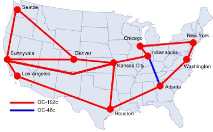
(a) Map of Abilene

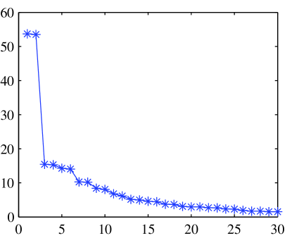
(b) Eigenspectrum of $G$

Figure 1: Map of the Abilene network and the eigenspectrum of one of its routing matrices.

A standard tool for assessing dimensionality and effective rank is the singular value decomposition (SVD) of $G$, which can be derived from an eigen-analysis of the matrix $B=G^{T}G$. The eigenvalues of $B$ (i.e., the squares of the singular values of $G$) are plotted in Figure 1(b). The large gap between the second and third eigenvalues, and the resulting knee in the spectrum, is evidence of a non-trivial amount of linear dependence among the rows of $G$. The effective rank of a matrix is determined by looking for a large gap in the spectrum that partitions the spectrum into large and small values. Thus the gap in Figure 1(b) suggests that as few as two paths may be sufficient to recover useful information about $y$ in the Abilene network.

Such strong spectral decay appears to be a common property of routing matrices. In Figure 2 we plot the spectra for five of the networks mapped by the Rocketfuel project [10]. The sharp knee that occurs roughly 20% of the way through is evidence that the effective rank of these routing matrices is much smaller then their actual rank. Furthermore, a remarkable amount of similarity can be seen in the decay of the five spectra.

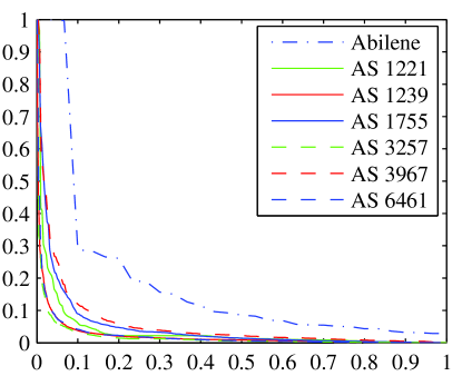
Figure 2: Spectra of $G$ for six networks mapped by the Rocketfuel project and Abilene. Note that the spectrum for each network has been re-scaled by the largest eigenvalue and the indices have been re-scaled to the unit interval. So on the horizontal axis, 1 corresponds to the $\operatorname{Rank}(G)$-th eigenvalue.

To better appreciate the connection between this spectral behavior and network path properties, we turn to the eigenvectors, which here may be viewed as orthogonal vectors that capture independent “patterns” that occur among the paths in $G$. For example, the first eigenvector corresponds to the “direction” in link space that maximizes the path volume of $y$, i.e., $v_{1}=\arg\max_{\lVert x\rVert=1}x^{T}G^{T}Gx=\arg\max_{\lVert x\rVert=1}y^{T}y$. As can be seen in Figure 3, the energy of the first eigenvector for Abilene is concentrated along an east-west “path” across the northern part of the network, with the greatest concentration of energy occurring at the centrally located Indianapolis-Kansas City link. The subsequent eigenvectors can be seen to bring in successive refinements to this picture, with the second and third eigenvectors further emphasizing connections to and within the “path” indicated by the first, while with the fourth eigenvector we begin to see evidence of a second east-west “path” along the southern part of the network. See [11] for additional discussion.

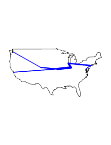
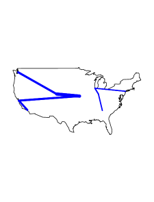
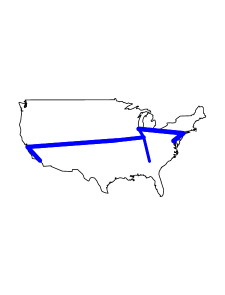
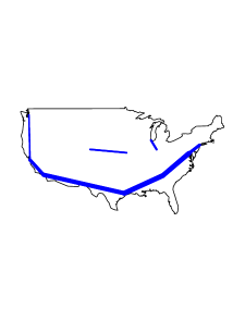
(a) (b) (c) (d)

Figure 3: First four distinct eigenvectors of $B=G^{T}G$ for Abilene. Each link is drawn with a thickness that is roughly proportional to the magnitude of its corresponding eigenvector component.

II-C Connection to Betweenness

The evidence in Figures 1(b) and 2 indicates that the effective rank of routing matrices in real networks can be noticeably lower than the actual rank. In the next section we will show how this phenomenon allows for substantial savings in measurement load for the particular problem of path monitoring that we have chosen to study. But we believe that the implications are in fact much broader. This would suggest that the issue of reduced rank is a topic worth better understanding in and of itself. For example, from a practical perspective, it would be useful to understand how decisions in network design and route management affect the relative change from actual to effective rank. In this regard, connections between the spectral decay of $G$, on the one hand, and known metrics of topological structure, on the other hand, are likely to be useful. While a comprehensive study of this sort is beyond the scope of the present paper, we describe here a result establishing a connection with one such metric.

Specifically, note that the plots in Figure 3 confirm our original intuitive notion that the effective rank of $G$ bears an intimate connection with the disproportionate role played by some links over others in the routing of paths within the network. This observation suggests the relevance of the concept of betweenness centrality, a concept fundamental in the literature on social networks [12] and more recently being used in the study of complex networks in the statistical physics literature (e.g., [13, 14]). Essentially, betweenness centrality measures the number of paths that utilize a specified node, in the case of ‘vertex centrality’, or a specified link, in the case of ‘edge centrality’.

Note that the diagonal elements of the matrix $B=G^{T}G$ are precisely the number of paths routed over their respective links and hence a measure of the centrality of each link in the network. The off-diagonal elements measure the number of paths routed simultaneously over pairs of links, and might therefore be termed a measure of edge ‘co-centrality’ or ‘co-betweenness’. The co-betweenness $B_{i,j}$ of any two edges $i$ and $j$ will always be bounded above by the smaller of the two edge betweenness’, i.e., $B_{i,j}\leq\min\{B_{i,i},B_{j,j}\}$. Hence, it might not be unreasonable to expect that the behavior of the eigen-spectrum of $B$ may be related to that of its diagonal, as the following result shows.

Proposition II.1

Let $B=G^{T}G$ and, without loss of generality, assume that the edges have been ordered so that $B_{1,1}\geq\dots\geq B_{n_{e},n_{e}}$. Then, for $k=1,\dots,n$, we have $\lambda_{k}\leq B_{k,k}\operatorname{diam}(\mathcal{G})$, and for $k>1$,

$$\frac{\lambda_{k}}{\lambda_{1}}\leq\frac{B_{k,k}}{B_{1,1}}\,\operatorname{diam}(\mathcal{G})\;,$$ (2)

where $\operatorname{diam}(\mathcal{G})$ is the diameter of the network graph $\mathcal{G}$.

Proof of this result may be found in Appendix A. The inequality in (2) indicates that the spectral decay in $G$ at worst parallels the decay of the edge betweenness on $\mathcal{G}$. In fact, examination of these quantities for the Rocketfuel datasets suggests that the decay in the $\lambda_{k}$ can be noticeably faster. Nevertheless, Proposition II.1 provides a connection through which recent and ongoing work on betweenness in complex networks (e.g., [13, 14]) may be found to have direct implications on the present context.

III Prediction of End-to-End Network Properties

In this paper, we take as our monitoring goal the task of obtaining accurate (approximate) knowledge of a linear summary of network path conditions. That is, we seek to accurately predict a linear function of the path conditions $y$, of the form $l^{T}y$ where $l\in\mathbf{R}^{n_{p}}$, based on measurements, say $y_{s}\in\mathbf{R}^{k}$, of a subset of $k$ paths. Two such linear summaries are the network-wide average, given by $l^{T}y$ for $l_{i}\equiv 1/n_{p}$, and the difference between the averages over two groups of paths $\mathcal{P}_{1}$ and $\mathcal{P}_{2}$, given by $l_{i}=1/\lvert\mathcal{P}_{1}\rvert$ for $i\in\mathcal{P}_{1}$ and $l_{i}=-1/\lvert\mathcal{P}_{2}\rvert$ for $i\in\mathcal{P}_{2}$. The prediction of $l^{T}y$ from the $k$ sampled path values in $y_{s}$ can be viewed as a particular instance of the classical problem of prediction in the statistical literature on sampling [15]. In this section, we (i) lay out our statistical framework, (ii) describe an accompanying path selection algorithm, and (iii) provide an analytical characterization of expected performance properties for our overall prediction methodology.

III-A Statistical prediction from sampled paths.

We begin by building a model for the end-to-end properties in $y$. In the work that follows, it is only necessary that the first two moments of $x$ and $y$ be specified, as opposed to a full distributional specification. Let $\mu$ be the mean of $x$ and let $\Sigma$ be the covariance of $x$. Then the corresponding statistics for $y$ are simply $\nu=G\mu$ and $V=G\Sigma G^{T}$, respectively.

Now fix $k\leq\operatorname{Rank}(G)$. Let $y_{s}\in\mathbf{R}^{k}$ denote the values $y_{i_{1}},\dots,y_{i_{k}}$ of the metric of interest for $k$ paths $i_{1},\dots,i_{k}\in\mathcal{P}$ that are to be sampled (i.e., measured), and let $y_{r}\in\mathbf{R}^{n_{p}-k}$ denote the values for those $n_{p}-k$ paths that remain. Similarly, let $G_{s}$ be those rows of $G$ corresponding to the $k$ paths, $i_{1},\dots,i_{k}$ and let $G_{r}$ be the remaining rows. We have thus partitioned $y$ and $G$ into $y=[y_{s}^{T},y_{r}^{T}]^{T}$ and $G=[G_{s}^{T},G_{r}^{T}]^{T}$, and we may similarly re-express the mean and covariance of $y$ as

$$\nu=\begin{bmatrix}\nu_{s}\\ \nu_{r}\end{bmatrix}=\begin{bmatrix}G_{s}\mu\\ G_{r}\mu\end{bmatrix}\quad\text{and}\quad V=\begin{bmatrix}V_{ss}&V_{sr}\\ V_{rs}&V_{rr}\end{bmatrix}=\begin{bmatrix}G_{s}\Sigma G_{s}^{T}&G_{s}\Sigma G_{r}^{T}\\ G_{r}\Sigma G_{s}^{T}&G_{r}\Sigma G_{r}^{T}\end{bmatrix}\text{.}$$ (3)

If the standard mean-squared prediction error (MSPE) is used to judge the quality of a predictor, i.e., if the quality of a predictor $p(y_{s})$ is measured by $\operatorname{MSPE}(p(y_{s}))\equiv E[(l^{T}y-p(y_{s}))^{2}]$, then the best predictor is known to be given by the conditional expectation $E[l^{T}y|y_{s}]=l_{s}^{T}y_{s}+E[l_{r}^{T}y_{r}|y_{s}]$, where $l=[l_{s}^{T},l_{r}^{T}]^{T}$ is partitioned in the same manner as $y$. But this predictor requires knowledge of the joint distributional structure. It is therefore common practice to restrict attention to a smaller and simpler subclass of predictors. A natural choice is the class of linear predictors, in which case, the best linear predictor (BLP) is given by the expression

$$a^{T}y_{s}=l_{s}^{T}y_{s}+l_{r}^{T}G_{r}\mu+l_{r}^{T}c_{*}(y_{s}-G_{s}\mu)\text{,}$$ (4)

where $c_{*}$ is any solution to $c_{*}V_{ss}=V_{rs}$. However, without knowledge of $\mu$, the BLP in (4) is an ideal that cannot be computed. One natural solution is to estimate $\mu$ from the data. Using generalized least squares, the mean can be estimated as $\hat{\mu}=[G_{s}^{T}V_{ss}^{-1}G_{s}]^{-}G_{s}^{T}V_{ss}^{-1}y_{s}$, where $M^{-}$ denotes a generalized inverse of a matrix $M$. Substituting $\hat{\mu}$ for $\mu$ in (4) produces an estimate of the BLP (an E-BLP) that is a function of only the measurements $y_{s}$, the routing matrix $G$ and the link covariance matrix $\Sigma$. Specifically, we obtain the predictor

$$\hat{a}^{T}y_{s}=l_{s}^{T}y_{s}+l_{r}^{T}G_{r}[G_{s}^{T}V_{ss}^{-1}G_{s}]^{-}G_{s}^{T}V_{ss}^{-1}y_{s}=l_{s}^{T}y_{s}+l_{r}^{T}V_{rs}V_{ss}^{-1}y_{s}\text{.}$$ (5)

The derivation of these and the other expressions above parallels that of similar linear prediction methods in spatial statistics—so-called ‘kriging’ methods—which motivates the name ‘network kriging’. An example of the basic underlying argument, in the case of simple linear statistical models, can be found in [16, pp. 225–227]. In the case of the present context, the derivation requires only that $V_{ss}$ be invertible and that $\Sigma$ be positive definite.

III-B Path Selection Algorithm

The material in Section III-A assumes a set of measurements from $k$ paths $i_{1},\ldots,i_{k}\in\mathcal{P}$. However, given the resources to measure any $k$ paths in a network, we are still faced with the question of which $k$ paths to measure. A natural response would be to choose $k$ paths that minimize $\operatorname{MSPE}(\hat{a}^{T}y_{s})$, over all subsets of $k$ paths. Standard manipulations yield that this quantity has the form

$$\operatorname{MSPE}(\hat{a}^{T}y_{s})=\underbrace{l_{r}^{T}\left(V_{rr}-V_{rs}V_{ss}^{-1}V_{sr}\right)l_{r}}_{\operatorname{MSPE}(a^{T}y_{s})}+\underbrace{l_{r}^{T}\left(V_{rs}V_{ss}^{-1}G_{s}-G_{r}\right)\mu}_{(\operatorname{Bias}\hat{a}^{T}y_{s})^{2}}.$$ (6)

Of course, since we typically do not know $\mu$, minimization of the full expression for $\operatorname{MSPE}(\hat{a}^{T}y_{s})$ is an unrealistic goal in practice. Instead, if adequate information on the covariance matrix $\Sigma$ is available, one might consider trying to minimize $\operatorname{MSPE}(a^{T}y_{s})$. A useful equivalent expression for this quantity is

$$\operatorname{MSPE}(a^{T}y_{s})=l_{r}^{T}(G_{r}C)(I-B_{s})(G_{r}C)^{T}l_{r}\,\text{,}$$ (7)

where $C$ is a nonsingular matrix satisfying $\Sigma=CC^{T}$, such as $\Sigma^{-\frac{1}{2}}$, and $B_{s}$ is the orthogonal projection matrix onto the span of the rows of $G_{s}C$, i.e., onto $\operatorname{Row}(G_{s}C)$. Since orthogonal projection matrices are idempotent and symmetric, the MSPE in (7) can be viewed as the square of the Euclidean norm of the projection of $(G_{r}C)^{T}l_{r}$ onto the complement of $\operatorname{Row}(G_{s}C)$, i.e., onto $\operatorname{Row}(G_{s}C)^{\perp}=\operatorname{Null}(G_{s}C)$.

In order to better appreciate the interpretation of (7), consider the special case of predicting a single unmeasured path (i.e., $l\equiv 0$ except for a single $1$ in $l_{r}$), with $\Sigma=I$. The MSPE in (7) then simply measures the extent to which the corresponding row of $G$ for this path lies outside of $\operatorname{Row}(G_{s})$. Similarly, the more interesting case of a non-trivial $l$ can be interpreted roughly as seeking a subset of $k$ paths for whom the rows in $G_{s}$ capture as many of the rows of $G$ as possible to the largest extent possible.

From the standpoint of optimization theory, our path-selection problem may be viewed as an example of the so-called ‘subset selection’ problem in computational linear algebra. In the case just described, and more generally for diagonal $\Sigma$, the selection of an appropriate subset of rows of $GC$ has a meaningful physical interpretation, in terms of the selection of paths, and vice versa. Exact solutions to this problem are computationally infeasible (it is known to be NP-complete), but the problem is well-studied and an assortment of methods for calculating approximate solutions abound.

The method we have used for the empirical work in this paper was adapted from the subset selection method described in Algorithm 12.1.1 of [9]. Essentially, our algorithm makes heuristic use of a QR-factorization with column pivoting to find $k$ rows of $G$ that approximate the span of the first $k$ left singular vectors of $GC$. The left singular vectors form an orthonormal basis for the range of $GC$ and the magnitude of their corresponding singular values indicates their relative importance. Note that these singular values are precisely the square-root of the eigenvalues of $(GC)^{T}(GC)$, i.e., the decaying spectrum from Section II. See [17] for additional details.

For a given choice of $k$, the overall complexity for the computation of the E-BLP in (5) is dominated by the computation of the SVD of $GC$, which is $O(n_{p}^{2}n_{e})$. This can likely be improved through the use of methods for sparse matrices, since the entries of $GC$ tend to include a large fraction of zeros. The other components of the computation are the QR-factorization with column pivoting, which is $O(k^{2}n_{p})$, and the computation of $V_{ss}^{-1}$ which is only $O(k^{3})$.

III-C Characterization of MSPE Properties

Analytical arguments are useful for characterizing the expected performance of a predictor resulting from the combination of equation (5) with an arbitrary subset selection algorithm. For example, we have the following bound.

Proposition III.1

Denoting the $i^{\text{th}}$ row of $G$ as $G_{(i)}$ , let $p_{i}=\lVert G_{(i)}\rVert_{2}^{2}/\lVert G\rVert_{F}^{2}$ , where $\lVert\cdot\rVert_{2}$ and $\lVert\cdot\rVert_{F}$ are the matrix 2-norm and the Frobenius matrix norm, respectively. Let $\tilde{G}_{s}$ be a rescaled version of $G_{s}$ , under the operation $G_{(i)}\rightarrow G_{(i)}/\sqrt{kp_{i}}$ , for each of the $k$ rows in $G_{s}$. Then if

$$\left\lVert G^{T}G-\tilde{G}_{s}^{T}\tilde{G}_{s}\right\rVert_{F}\leq f(k)\left\lVert G\right\rVert_{F}^{2}\enskip,$$ (8)

for some $f(k)$, the MSPE can be bounded as

$$\operatorname{MSPE}(\hat{a}^{T}y_{s})\leq(\left\lVert\mu\right\rVert_{2}^{2}+1)\left(\lambda_{k+1}+2f(k)\left\lVert G\right\rVert_{F}^{2}\right)\left\lVert l\right\rVert_{2}^{2}\text{.}$$ (9)

Proof of this result may be found in Appendix B. The inequality in (9) shows that the decay of the MSPE in $k$ is controlled by two factors. The first factor, $\lambda_{k+1}$, quantifies how well $G$ may be approximated by its first $k$ singular dimensions, and will be small when $k$ is no smaller than the effective rank of $G$. The second factor, $f(k)$, quantifies the ability of the underlying subset selection algorithm to approximate $G$ by a matrix $G_{s}$ formed from $k$ of its rows. Our empirical experience indicates that in practice $\lambda_{k+1}$ can be much smaller than the term involving $f(k)$, which suggests that the rate of decay is dominated by $f(k)$.

To get an idea of the behavior of $f(k)$ for real networks, we computed $\left\lVert G^{T}G-\tilde{G}_{s}^{T}\tilde{G}_{s}\right\rVert_{F}/\lVert G\rVert_{F}^{2}$ for the Abilene backbone and five networks mapped by the Rocketfuel project, for the subset selection algorithm described in Section III-B. As can be seen in Figure 4, there is a strong power-law decay in $\left\lVert G^{T}G-\tilde{G}_{s}^{T}\tilde{G}_{s}\right\rVert_{F}/\lVert G\rVert_{F}^{2}$, with an exponent that ranges from $-0.49$ to $-0.53$. The consistency in this decay is quite remarkable, as it says that our subset selection algorithm finds a similarly good set of paths, for each $k$, in each of the networks. That this decay in $f(k)$ indeed translates into good MSPE properties will be seen in Section IV.

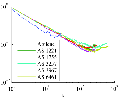
Figure 4: Plot of $\left\lVert G^{T}G-\tilde{G}_{s}^{T}\tilde{G}_{s}\right\rVert_{F}/\lVert G\rVert_{F}^{2}$ for the Abilene backbone and Rocketfuel networks.

Proposition III.1 holds for any given deterministic path selection algorithm. Perhaps surprisingly, it is possible to state a similar result for a randomized path selection algorithm. The empirical work we present in the next section clearly establishes the practical effectiveness of our methodology using the deterministic algorithm described in Section III-B. However, effective randomized path selection algorithms are interesting to consider in the sense that such algorithms would be able to reduce the likelihood that small, highly localized events consistently remain outside the span of the sampled paths. The following result, the proof of which follows as a direct corollary of Theorem 3 in [18], suggests that an algorithm that randomly selects paths roughly in proportion to path length could indeed achieve similar performance characteristics.

Proposition III.2

Let $\tilde{G}_{s}$ be a matrix constructed as in Proposition III.1, but now from $c$ paths randomly selected (with replacement) with respect to the probabilities $\{p_{i}\}$. If the estimator $\hat{a}^{T}y_{s}$ in (5) is constructed based on the first (at most) $k\leq c$ singular dimensions of $\tilde{G}_{s}$, then for any $c\leq n_{p}$ and $\delta>0$,

$$MSPE(\hat{a}^{T}y_{s})\leq(\lVert\mu\rVert_{2}^{2}+1)(\lambda_{k+1}+2(1+\sqrt{\ln(2/\delta)})c^{-\frac{1}{2}}\,\lVert G\rVert_{F}^{2})\,\lVert l\rVert_{2}^{2}$$ (10)

holds with probability at least $1-\delta$.

IV Empirical Validation of Prediction Methodology

In this section, we show how our framework may be applied to address two practical problems of interest to network providers and customers. In particular, we show how the appropriate selection of small sets of path measurements can be used to (i) accurately estimate network-wide averages of path delays, and (ii) reliably detect network delay anomalies. We first describe the assembly of our dataset, and then present the two applications.

IV-A Data: Abilene Path Delays

Our methods are applicable to any per-link metric that adds to form per-path metrics. As a specific example, we consider delay. In order to validate our prediction methodology, we constructed a full set of path-delay data for the Abilene network, using measurements obtained from the NLANR Active Measurement Project (AMP). This project continually performs traceroutes between all pairs of AMP monitors on ten minute intervals. Because most AMP monitors are on networks with Abilene connections, most traceroutes pass over Abilene. These data thus provide a highly detailed view of the state of the Abilene network.

Beginning with a full set of measurements taken over 3 days in 2003, our approach to constructing per-path delays from this data consisted of (i) estimating per-link delays $x^{(t)}\in\mathbf{R}^{30}$ across the 30 network links, for each consecutive ten minute epoch $t$, and (ii) computing the per-path delays from these per-link delays, on the 110 Abilene paths, using the relation $y^{(t)}=Gx^{(t)}$, where $G$ is a fixed routing matrix corresponding to the routing on Abilene at the start of the 3 day period. The end result is a temporally indexed sequence of path-delay vectors $y^{(t)}$ over $432$ successive epochs during the 3 day period. Note that the inferred link delays $x^{(t)}$ are not explicitly used by our prediction methodology, but rather were only necessary for the construction of the path delays, after which they were discarded.

To construct the link delays, for each epoch $t$, we started with traceroutes between the 14,917 pairs of AMP monitors for which complete data were available. Links comprising the Abilene network were identified by their known interface addresses. Since different traceroutes traverse each link at slightly different times, and since each traceroute takes up to three measurements per hop, we formed a single estimate of each link’s delay by averaging across all the traceroutes that measured that link in the current epoch. This approach yields a single measure of delay for each link and epoch; while this measure does not capture the variations in delay that occur within a ten minute interval, it provides a realistic and representative value for delay that is sufficient for our validation purposes.

Recall that the statistical framework in Section III-A involved only the first two moments of the link delays, the mean $\mu$ and the covariance $\Sigma$. While our methodology does not require knowledge of $\mu$, since it is estimated at each epoch interval as part of the calculation of our predictor, we note here that the mean delays in our data for Abilene’s $30$ directed edges were fairly uniform over the interval from 2 to 36 milliseconds, with standard deviations that ran from 0.16 to 0.94 over the full three-day period. Our methodology does, however, require knowledge of $\Sigma$, which in practice must be elicited from either historical data or possibly periodic, infrequent measurements on the links. For the purposes of the validation in this section, we used the per-link delays $x^{(t)}$ for one day’s worth of data to obtain an estimate of $\Sigma$. The entries in this matrix were found to be primarily dominated by the diagonal elements, with only a small number of off-diagonal entries of similar magnitude. Inspection of the actual delay data suggested that the majority of the latter were due to artifacts of the measurement procedure. Therefore, in implementing our methodology we took $\Sigma$ to be the corresponding diagonal matrix. See [17] for additional details, including evidence regarding the improvement gained over the choice $\Sigma\propto I$.

IV-B Monitoring a Network-Wide Average

An average is perhaps the most basic network-wide quantity that one might be interested in monitoring. So as our first application, we consider the prediction of the average delay over all $n_{p}=110$ Abilene paths as a function of time $t$, i.e., $l^{T}y^{(t)}$ with $l_{i}\equiv 1/n_{p}$, $i=1,\ldots,n_{p}$, and $t=1,\ldots,432$. Using (5), we computed predictions of the network-wide average path delay during each epoch, for a choice of $k=1,\ldots,30$ measured paths. The paths were chosen using the algorithm described in Section III-B. To summarize the accuracy of our predictions, we calculated the average relative error for each $k$, where the average is taken all the 432 epochs. The results are shown in Figure 5.

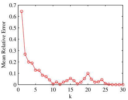
Figure 5: Mean relative prediction error as a function of $k$.

Recall that exact recovery of all paths delays $y^{(t)}$, at a given epoch $t$, requires measurement of $k^{*}=\operatorname{Rank}(G)$ paths, which in this case means $k^{*}=30$. In examining Figure 5, note that in comparison a relative error of roughly only $10\%$ is achievable using only $k=7$ path measurements. Increasing $k$ further improves the accuracy of the prediction up until around $k=9$ or $10$, after which it basically levels out. Since it is roughly at this point that the spectra of the (weighted) routing matrices level out as well, this suggests that our subset selection algorithm is indeed doing what we are asking of it, in that it is tracking the effective rank quite closely. Additional results of this sort, on a variety of simulated datasets, may be found in [11].

To get a better idea of how well the predictors performed, we can compare plots of the predictions against a plot of the actual mean delays, as shown in Figure 6 for $k=3,5,7$ and $9$. Note that all of the predictions mirror the rise and fall of the actual network-wide delay quite closely—even for $k=3$ measured paths the correlation with the data time-series is $\rho=0.814$. However, it is also clear that there is a downward bias in these predictions, and that this bias is increasingly prominent as $k$ decreases.

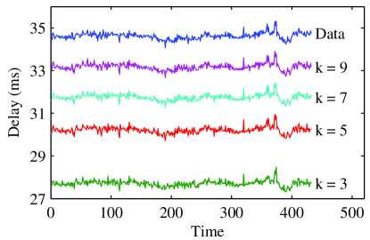
Figure 6: Predictions of network-wide average path delays, for various choices of $k$.

The source of this bias can be traced to a lack of information on links in the network that are traversed by none of the $k$ measured paths. In fact, the generalized inverse used in our E-BLP in (5) simply estimates the corresponding values $x_{j}$ on these links to be zero. Hence, as we reach a point where every link contributes to at least one measured path, as it does by roughly $k=10$, the bias diminishes accordingly. Note, however, that the bias for each $k$ in Figure 6 is fairly constant. This suggests that a small amount of additional measurement information could go a long way.

We implemented a simple method of bias correction, that uses a one-time measurement of a sufficient set of paths for complete reconstruction of the link delays (in this case, 30 paths). Since it is a one-time-only measurement, it represents a minimal addition to the network measurement load. The bias of our prediction for the first epoch was then calculated and used to adjust the predictions in the other 431 epochs, which amounts to a simple shift upward of each curve in Figure 6. Boxplots of the relative bias remaining after application of this procedure are shown in Figure 7. The predictions are now extremely accurate, usually being off by less than $0.3\%$, and almost always within $1\%$—even when as few as $k=3$ paths are measured.

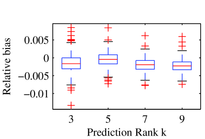
Figure 7: Relative bias after bias correction.

Before moving on, we note that this performance on whole networks extends to subnetworks. In particular, we have successfully used our methods to make reliable comparisons between sub-network delays in the context of multi-homing [17].

IV-C Anomaly Detection

The application in Section IV-B evaluates our predictor by standard statistical summaries, in essence looking at the accuracy of the predictor at hitting an unknown target. But it is also important to evaluate the accuracy in terms of accomplishing higher-level tasks. One such higher-level task of importance is the detection of potentially anomalous events.

For the purposes of illustration with our Abilene delay data, we define an anomaly as a spike in the network-wide average path delay that deviates from the mean of the previous six values (i.e., one hour) by more than a prescribed amount. For example, the dots in Figure 9 indicate points at which the average path delay differs from the mean of the previous six epochs by more than three times their standard deviation.

To predict when such anomalies occur, we look for spikes in the predicted average path delay, calculated as described in Section IV-B and using a user-defined threshold. It is interesting to examine the effect of choice of both $k$ and this threshold parameter. Insight can be obtained by examining ROC (Receiver Operating Characteristic) curves such as those in Figure 8. Such plots, showing the true positive rate against the false positive rate for different parameter values, are a common tool for establishing cutoff values for detection tests. Each curve in Figure 8 is formed by taking one value for $k$ and varying the threshold level. Examining these curves, one sees that for a given threshold, say $1\sigma$, the true positive rate increases with the sample size $k$ while the false positive rate stays about the same. Working with a $k=9$ prediction, we see that the upper-left corner of the ROC curve (the best trade-off between a low false positive rate and a high true positive rate) occurs at around $2\sigma$.

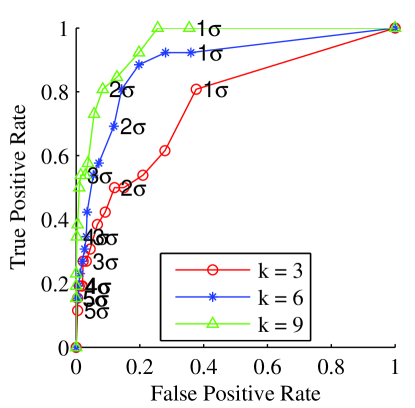
Figure 8: ROC curves for predicting $3\sigma$ spikes. The threshold used to predict the spikes is varied from $1\sigma$ to $5\sigma$ in increments of $0.25\sigma$.

In Figure 9, the results are shown for the case $k=9$, with a threshold of $2\sigma$. Circles have been placed along the actual path delay time series at the epochs that were flagged as anomalies in the predicted time series. On the whole, this predictor is quite accurate. Most of the major spikes are flagged, resulting in a true positive rate of 81%, while the false positive rate is only 8%. Furthermore, most of these false positives seem to occur at lesser spikes in the actual delay data.

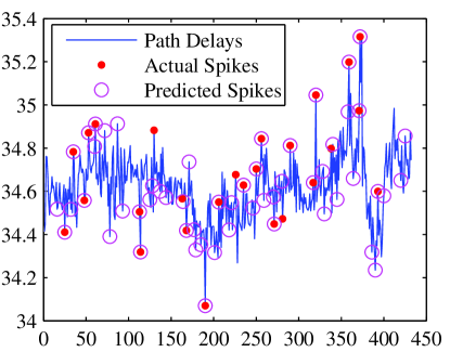
Figure 9: Comparison of predicted and actual spikes. The real spikes are those that exceed 3 times the standard deviation of the previous 6 epochs. The predicted spikes are those epochs where the rank 9 prediction exceeds 2 times the standard deviation of its previous 6 epochs.

V Discussion

The identification of an inherent statistical prediction problem in the task of end-to-end network path monitoring—which we have dubbed ‘network kriging’—is analogous in its potential impact with the identification of, say, traffic matrix estimation with tomography (i.e., ‘network tomography’). In both cases, the identification serves as a critical pointer to an already established literature, through which methodology may be developed by leveraging various principles and tools. Here we have focused exclusively on one basic version of the network kriging problem, the prediction of linear metrics of path properties using linear modeling principles. However, there is ample room for work beyond this, including for example extensions to non-linear metrics and temporal prediction models.

We have successfully demonstrated the promise of our proposed methodology on data obtained from a real network. Nevertheless, there are various practical issues to be dealt with to optimize our framework for full-scale implementation. These include efficient strategies for dealing with monitor failures, link failures and routing changes. We expect that many of these may be addressed using tactics similar to those proposed in [7].

On a final note, we mention again the fundamental importance of the material in Section II-B, on the prevalence of low effective rank of routing matrices, to the success of our methodology. Put simply, low effective rank allows for the possibility of effective network-wide monitoring with reduced measurement sets. While we have exploited this characteristic for the purpose of path monitoring, it should apply equally well when the goal involves selective monitoring of links. The driving factors responsible for the low effective rank are poorly understood and remain an interesting open problem.

Appendix A Proof of Proposition II.1.

Let $\lambda_{1}\geq\dots\geq\lambda_{n}$ denote the eigenvalues of the matrix $B$ and define the spectral radius of $B=G^{T}G$ as $\rho(B)=\max\{\lvert\lambda_{1}\rvert,\dots,\lvert\lambda_{n}\rvert\}=\lambda_{1}$. Now partition the matrix $B$ into $B=\bigl{[}\begin{smallmatrix}E&C^{T}\\ C&F^{\phantom{T}}\end{smallmatrix}\bigr{]}$ where $F$ is an $m\times m$ matrix with $m<n_{e}$ whose diagonal elements are the $m$ smallest betweennesses. Denote the eigenvalues of $F$ by $\theta_{1}\geq\dots\geq\theta_{m}$ and, for convenience, let $\theta_{i}=-\infty$ for $i>m$ and $\theta_{i}=\infty$ for $i\leq 0$. Cauchy’s Interlace Theorem tells us that the $m$ eigenvalues of $F$ are upper bounds for the $m$ smallest eigenvalues of $B$, respectively.

For the moment, we focus on the case of $\theta_{1}\geq\lambda_{n-m+1}$. If we can bound $\theta_{1}$ we will have a bound for $\lambda_{n-m+1}$. Define the $i$-th row sum of $B$ as $r_{i}(B)=\sum_{j=1}^{n}\lvert B_{i,j}\rvert$, and the deleted row sum of $B$ as $\tilde{r}_{i}(B)=\sum_{\begin{subarray}{c}j=1\\ j\neq i\end{subarray}}^{n}\lvert B_{i,j}\rvert$. It then follows, by way of a corollary to Gershgorin’s Theorem[19], that the spectral radius of $F$ is bounded by

$$\rho(F)\leq\max_{1\leq i\leq m}r_{i}(F)\leq\max_{n-m+1\leq i\leq n}r_{i}(B)\;.$$ (11)

Each of these row sums $r_{i}(B)$ can be bounded in terms of the diagonal element $B_{i,i}$. To see this, note that each of the $B_{i,i}$ paths that use edge $i$ have a length of at most $\operatorname{diam}(\mathcal{G})$. So each path can contribute at most $\operatorname{diam}(\mathcal{G})$ to the row sum $r_{i}(B)$. This means that for a betweenness matrix $B$ we have $r_{i}(B)\leq B_{i,i}\,\operatorname{diam}(\mathcal{G})$. Recalling that we have ordered the edges such that the diagonal elements $B_{i,i}$ are non-increasing, our bound for the spectral radius becomes

$$\rho(F)\leq B_{n-m+1,n-m+1}\operatorname{diam}(\mathcal{G})\;.$$ (12)

Which means that our bound for the eigenvalue of $B$ is

$$\lambda_{n-m+1}\leq\theta_{1}\leq r_{n-m+1}(B)\leq B_{n-m+1,n-m+1}\,\operatorname{diam}(\mathcal{G})\,.$$ (13)

Finally, note that we are free to choose $m=1,\dots,n-1$. So for $i=2,\dots,n$ we have an upper bound that decays no worse than the betweenness $B_{i,i}$, namely,

$$\lambda_{i}\leq B_{i,i}\operatorname{diam}(\mathcal{G})\;.$$ (14)

The $i=1$ case follows from Gershgorin applied directly to $B$.

To establish the second bound, given in (2) of Proposition II.1, note that for any unit vector $u$ we have $\lVert Bu\rVert_{2}\leq\lambda_{1}$. In particular, for $u=e_{1}=[1,0,\dots,0]^{T}$ we have $\lVert Be_{1}\rVert_{2}\leq\lambda_{1}$. Since $Be_{1}$ is the first column of $B$, we have $\lVert Be_{1}\rVert_{\infty}=B_{1,1}$. Thus $B_{1,1}=\lVert Be_{1}\rVert_{\infty}\leq\lVert Be_{1}\rVert_{2}=\lambda_{1}$. Dividing the left and right-hand sides of (14) by $\lambda_{1}$ and $B_{1,1}$, respectively yields the desired bound.

Appendix B Proof of Proposition III.1.

Since $\operatorname{MSPE}(\hat{a}^{T}y_{s})=\left\lVert\mu^{T}(I-B_{s})G^{T}l\right\rVert_{2}^{2}+\left\lVert(I-B_{s})G^{T}l\right\rVert_{2}^{2}\leq(\left\lVert\mu\right\rVert_{2}^{2}+1)\,\lVert(I-B_{s})G^{T}\rVert_{2}^{2}\,\left\lVert l\right\rVert_{2}^{2}$, we need only show $\lVert(I-B_{s})G^{T}\rVert_{2}^{2}\leq\lambda_{k+1}+2f(k)\lVert G\rVert_{F}^{2}$. To do so, we proceed as in the proof of Theorem 3 in [18]. Note that for any vector $x\in\mathbf{R}^{n}$ with $\left\lVert x\right\rVert=1$ we can write $x=ay+bz$, where $y\in\mathcal{S}_{s}=\operatorname{Row}(G_{s})$, $z\in\mathcal{S}_{s}^{\perp}$, $a,b\in\mathbf{R}$, and $a^{2}+b^{2}=1$. Using this decomposition of $x$ and the sub-linearity of the $2$-norm we can write

$$\left\lVert G^{T}-B_{s}G^{T}\right\rVert_{2} =\max_{\left\lVert x\right\rVert=1}\left\lVert x^{T}(G^{T}-B_{s}G^{T})\right\rVert$$ (15)

$$\leq\max_{\begin{subarray}{c}y\in\mathcal{S}_{s}\\ \left\lVert y\right\rVert=1\end{subarray}}\left\lVert y^{T}(G^{T}-B_{s}G^{T})\right\rVert+\max_{\begin{subarray}{c}z\in\mathcal{S}_{s}^{\perp}\\ \left\lVert z\right\rVert=1\end{subarray}}\left\lVert z^{T}(G^{T}-B_{s}G^{T})\right\rVert$$ (16)

At this point, we note that since $y\in\mathcal{S}_{s}$ we have $y^{T}B_{s}=y^{T}$, which means that $y^{T}(G^{T}-B_{s}G^{T})=0$. Furthermore, $z\in\mathcal{S}_{s}^{\perp}$ means that $z^{T}B_{s}=0$. So the upper bound becomes

$$\left\lVert G^{T}-B_{s}G^{T}\right\rVert_{2}\leq\max_{\begin{subarray}{c}z\in\mathcal{S}_{s}^{\perp}\\ \left\lVert z\right\rVert=1\end{subarray}}\left\lVert z^{T}G^{T}\right\rVert.$$ (17)

We can bound the maximum in (17) in terms of $\tilde{G}_{s}$ by

$$\lVert z^{T}G^{T}\rVert_{2}^{2}=z^{T}(G^{T}G-\tilde{G}_{s}^{T}\tilde{G}_{s})z+z^{T}\tilde{G}_{s}^{T}\tilde{G}_{s}z\leq\lVert G^{T}G-\tilde{G}_{s}^{T}\tilde{G}_{s}\rVert_{F}+\sigma_{k+1}^{2}(\tilde{G}_{s})\text{,}$$ (18)

where $\sigma^{2}_{k+1}(M)\equiv\lambda_{k+1}(M)$, since $\lVert z\rVert_{2}=1$ and $\lVert M\rVert_{2}\leq\lVert M\rVert_{F}$. Combining (17) and (18) gives us

$$\left\lVert G^{T}-B_{s}G^{T}\right\rVert_{2}^{2}\leq\sigma_{k+1}^{2}(\tilde{G}_{s})+\left\lVert G^{T}G-\tilde{G}_{s}^{T}\tilde{G}_{s}\right\rVert_{F}.$$ (19)

Turning to Corollary 8.6.2 in [9, p. 449] we have for $k=1,\dots,n_{e}$

$$\lvert\sigma_{k+1}(G^{T}G)-\sigma_{k+1}(\tilde{G}_{s}^{T}\tilde{G}_{s})\rvert\leq\lVert G^{T}G-\tilde{G}_{s}^{T}\tilde{G}_{s}\rVert_{2}.$$ (20)

Using the bound for $\lVert G^{T}G-\tilde{G}_{s}^{T}\tilde{G}_{s}\rVert_{F}$ that we are given in (8), and the relation $\lVert M\rVert_{2}\leq\lVert M\rVert_{F}$ for any matrix $M$ we have

$$\lVert G^{T}G-\tilde{G}_{s}^{T}\tilde{G}_{s}\rVert_{2}\leq f(k)\,\lVert G\rVert_{F}^{2}.$$ (21)

Thus $\lvert\sigma_{k+1}(G^{T}G)-\sigma_{k+1}(\tilde{G}_{s}^{T}\tilde{G}_{s})\rvert=\lvert\sigma_{k+1}^{2}(G)-\sigma_{k+1}^{2}(\tilde{G}_{s})\rvert\leq\left\lVert G^{T}G-\tilde{G}_{s}^{T}\tilde{G}_{s}\right\rVert_{2}\leq f(k)\,\lVert G\rVert_{F}^{2}$, which leads us to $\sigma_{k+1}^{2}(\tilde{G}_{s})\leq f(k)\left\lVert G\right\rVert_{F}^{2}+\sigma_{k+1}^{2}(G)$. Combined with (19) and (21) this yields that $\left\lVert(I-B_{s})G^{T}\right\rVert_{2}^{2}\leq\lambda_{k+1}+2f(k)\left\lVert G\right\rVert_{F}^{2}$, as was to be shown.

References

- [1] NLANR Active Measurement Project. [Online]. Available: http://amp.nlanr.net/AMP/
- [2] RIPE Test-Traffic Project. [Online]. Available: http://www.ripe.net/test-traffic/
- [3] Internet End-to-end Performance Monitoring Project. [Online]. Available: http://www-iepm.slac.stanford.edu/
- [4] Y. Chen, D. Bindel, and R. H. Katz, “Tomography-based overlay network monitoring,” in Proc. 2003 ACM SIGCOMM Conference on Internet Measurement. ACM Press, 2003, pp. 216–231.
- [5] Y. Shavitt, X. Sun, A. Wool, and B. Yener, “Computing the unmeasured: An algebraic approach to internet mapping,” in Proc. IEEE INFOCOM 2001, Apr. 2001.
- [6] N. A. C. Cressie, Statistics for Spatial Data, ser. Wiley Series in Probability and Mathematical Statistics: Applied Probability and Statistics. New York: John Wiley & Sons Inc., 1993.
- [7] Y. Chen, D. Bindel, H. Song, and R. H. Katz, “An algebraic approach to practical and scalable overlay network monitoring,” in Proc. 2004 ACM SIGCOMM. ACM Press, 2004.
- [8] H. X. Nguyen and P. Thiran, “Active measurement for multiple link failures: Diagnosis in IP networks,” in Proc. Passive and Active Measurements Workshop. Springer Verlag, 2004.
- [9] G. H. Golub and C. van Loan, Matrix Computations, 2nd ed. London: The Johns Hopkins University Press, 1989.
- [10] N. Spring, R. Mahajan, and D. Wetherall, “Measuring ISP topologies with Rocketfuel,” in Proc. ACM SIGCOMM 2002, 2002.
- [11] D. B. Chua, E. D. Kolaczyk, and M. Crovella, “Efficient estimation of end-to-end network properties,” in Proc. IEEE INFOCOM 2005, 2005.
- [12] S. Wasserman and K. Faust, Social Network Analysis: Methods and Applications. Cambridge University Press, Nov. 1994.
- [13] M. Barthélemy, “Betweenness centrality in large complex networks,” The European Physical Journal B, vol. 38, pp. 163–168, 2004.
- [14] M. E. J. Newman and M. Girvan, “Finding and evaluating community structure in networks,” Physical Review E, vol. 69, no. 2, p. 026113, Feb. 2004.
- [15] R. Valliant, A. H. Dorfman, and R. M. Royall, Finite Population Sampling and Inference: A Prediction Approach. Wiley Interscience, 2000.
- [16] R. Christensen, Plane Answers to Complex Questions. New York: Springer-Verlag, 1987.
- [17] D. B. Chua, E. D. Kolaczyk, and M. Crovella, “A statistical framework for efficient monitoring of end-to end network properties.” [Online]. Available: http://arxiv.org/abs/cs.NI/0412037
- [18] P. Drineas, A. Frieze, R. Kannan, S. Vempala, and V. Vinay, “Clustering large graphs via the singular value decomposition,” Machine Learning, vol. 56, no. 1–3, pp. 9–33, July 2004.
- [19] R. S. Varga, Geršgorin and His Circles, ser. Springer Series in Computational Mathematics. Berlin: Springer-Verlag, 2004, vol. 36.