Secondary terms in the number of vanishings of quadratic twists of elliptic curve $L$-functions

Abstract

We examine the number of vanishings of quadratic twists of the $L$-function associated to an elliptic curve. Applying a conjecture for the full asymptotics of the moments of critical $L$-values we obtain a conjecture for the first two terms in the ratio of the number of vanishings of twists sorted according to arithmetic progressions.

1 Introduction

Let $E$ be an elliptic curve over $\mathbb{Q}$ with associated $L$-function given by

$$L_{E}(s) =\sum_{n=1}^{\infty}\frac{a_{n}}{n^{s}}=\prod_{p\mid\Delta}\left(1-a_{p}p^{-s}\right)^{-1}\prod_{p\nmid\Delta}\left(1-a_{p}p^{-s}+p^{1-2s}\right)^{-1}$$ (1)

$$=\prod_{p}{\mathcal{L}}_{p}(1/p^{s}),\quad\quad\Re(s)>3/2.$$ (2)

Here, $\Delta$ is the discriminant of $E$, and $a_{p}=p+1-\#E(\mathbb{F}_{p})$, with $\#E(\mathbb{F}_{p})$ the number of points, including the point at infinity, of $E$ over $\mathbb{F}_{p}$. $L_{E}(s)$ has analytic continuation to $\mathbb{C}$ and satisfies a functional equation [12] [11] [1] of the form

$$\left(\frac{2\pi}{\sqrt{Q}}\right)^{-s}{\rm\Gamma}(s)L_{E}(s)=w_{E}\left(\frac{2\pi}{\sqrt{Q}}\right)^{s-2}{\rm\Gamma}(2-s)L_{E}(2-s),$$ (3)

where $Q$ is the conductor of the elliptic curve $E$ and $w_{E}=\pm 1$.

Let

$$L_{E}(s,\chi_{d})=\sum_{n=1}^{\infty}\frac{a_{n}\chi_{d}(n)}{n^{s}}$$ (4)

be the $L$-function of the elliptic curve $E_{d}$, the quadratic twist of $E$ by the fundamental discriminant $d$. If ($d,Q)=1$, then $L_{E}(s,\chi_{d})$ satisfies the functional equation

$$\left(\frac{2\pi}{\sqrt{Q}|d|}\right)^{-s}{\rm\Gamma}(s)L_{E}(s,\chi_{d})=\chi_{d}(-Q)w_{E}\left(\frac{2\pi}{\sqrt{Q}|d|}\right)^{s-2}{\rm\Gamma}(2-s)L_{E}(2-s,\chi_{d}).$$ (5)

In [5] and [6] conjectures, modeled after corresponding theorems in random matrix theory, are stated concerning the distribution of values of $L_{E}(1,\chi_{d})$ with an application made to counting the number of vanishings of $L_{E}(1,\chi_{d})$. We focus on the case $w_{E}\chi_{d}(-Q)=1$, since otherwise $L_{E}(1,\chi_{d})$ is trivially equal to zero. One quantity studied concerns the ratio of the number of vanishings sorted according to residue classes mod $q$ for a fixed prime $q\nmid Q$. Let

$$R_{q}(X)=\frac{\sum_{{|d|<X,w_{E}\chi_{d}(-Q)=1\atop L_{E}(1,\chi_{d})=0}\atop\chi_{d}(q)=1}1}{\sum_{{|d|<X,w_{E}\chi_{d}(-Q)=1\atop L_{E}(1,\chi_{d})=0}\atop\chi_{d}(q)=-1}1}$$ (6)

be the ratio of the number of vanishings of $L_{E}(1,\chi_{d})$ sorted according to whether $\chi_{d}(q)=1$ or $-1$.

By looking at this ratio, certain elusive and mysterious quantities that appear in the asymptotics for both the numerator and denominator cancel each other out and one is left with a precise prediction for its limit. Let

$$R_{q}=\left(\frac{q+1-a_{q}}{q+1+a_{q}}\right)^{1/2}.$$ (7)

A conjecture from [5] asserts that, for $q\nmid Q$,

$$\lim_{X\rightarrow\infty}R_{q}(X)=R_{q}.$$ (8)

It is believed that this continues to hold if the set of quadratic twists is restricted to subsets such as $d<0$ or $d>0$, or to $|d|$ prime, though in the latter case we must be sure to rule out there being no vanishings at all due to arithmetic reasons [7].

Numerical evidence for three elliptic curves is presented in [5] and confirms this prediction. However, even taking $X$ of size roughly $10^{9}$ (and, in that paper, $d<0$ and $|d|$ prime), the numeric value of the ratio was found in that paper to agree with the predicted value to about two decimal places. In other cases, when $a_{q}$ of $L_{E}(S)$ in (1) equals 0, the numeric value of $R_{q}(X)$ compared to the predicted limit $R_{q}$ to three or more decimal places.

In this paper we examine secondary terms in the above conjecture applying new conjectures [4] for the full asymptotics of the moments of $L_{E}(1,\chi_{d})$. We obtain a conjectural formula for the next to leading term in the asymptotics for $R_{q}(X)$. It is of size $O(1/\log(X))$ and explains the slow convergence to the limit $R_{q}$. We also explain in Section 3 the tighter fit when $a_{q}=0$.

While the main term, $R_{q}$, in the above conjecture is robust and does not depend heavily on the set of $d$’s considered, the secondary terms are more sensitive, for example, to the residue classes of $d$ modulo the primes that divide $Q$. Therefore, for simplicity we focus on the following dense collection of fundamental discriminants $d$. Assume that $Q$ is squarefree and let

$$S^{-}(X)=S^{-}_{E}(X)=\{-X\leq d<0;\chi_{d}(p)=-a_{p}\ \ \text{for all $p\mid Q$}\}$$ (9)

For curves of prime conductor $Q$ we also consider the set of fundamental discriminants

$$S^{+}(X)=S^{+}_{E}(X)=\{0<d\leq X;\chi_{d}(Q)=a_{Q}\}.$$ (10)

These sets of discriminants are also chosen because they allow us to efficiently compute $L_{E}(1,\chi_{d})$ using a relationship to the coefficients of certain modular forms of weight $3/2$ that has been worked out explicitly for many examples by Tornaria and Rodiguez-Villegas [9] (see [6] for more details). The sets $S^{\pm}(X)$ restrict $d$ according to certain residue classes mod $Q$ in the case that $Q$ is odd and squarefree, and $4Q$ in the case that $Q$ is even and squarefree.

2 Moments of $L_{E}(1,\chi_{d})$

Let

$$M^{\pm}_{E}(X,k)=\frac{1}{\left|S^{\pm}(X)\right|}\sum_{d\in S^{\pm}(X)}L_{E}(1,\chi_{d})^{k}.$$ (11)

be the $k$th moment of $L_{E}(1,\chi_{d})$.

The conjecture of Conrey-Farmer-Keating-Rubinstein-Snaith [4, 4.4] says here that, for $k\geq 1$, $k\in\mathbb{Z}$,

$$M^{\pm}_{E}(X,k)=\frac{1}{X}\int_{0}^{X}\Upsilon^{\pm}_{k}\left(\log(t)\right)dt+O(X^{-\tfrac{1}{2}+\epsilon})$$ (12)

as $X\rightarrow\infty$, where $\Upsilon_{k}$ is the polynomial of degree $k(k-1)/2$ given by the $k$-fold residue

$$\Upsilon^{\pm}_{k}(x) = \frac{(-1)^{k(k-1)/2}2^{k}}{k!}\frac{1}{(2\pi i)^{k}}$$

$$\times\oint\cdots\oint\frac{F^{\pm}_{k}(z_{1},\ldots,z_{k})\Delta(z_{1}^{2},\ldots,z_{k}^{2})^{2}}{\prod_{j=1}^{k}z_{j}^{2k-1}}e^{x\sum_{j=1}^{k}z_{j}}dz_{1}\ldots dz_{k},$$

where the contours above enclose the poles at $z_{j}=0$ and

$$F^{\pm}_{k}(z_{1},\ldots,z_{k})=A^{\pm}_{k}(z_{1},\ldots,z_{k})\prod_{j=1}^{k}\left(\frac{\Gamma(1+z_{j})}{\Gamma(1-z_{j})}\left(\frac{Q}{4\pi^{2}}\right)^{z_{j}}\right)^{\tfrac{1}{2}}\prod_{1\leq i<j\leq k}\zeta(1+z_{i}+z_{j}).$$ (14)

$A^{\pm}_{k}$, which depends on $E$, is the Euler product which is absolutely convergent for $\sum_{j=1}^{k}|z_{j}|<1/2$,

$$A^{\pm}_{k}(z_{1},\dots,z_{k})=\prod_{p}F^{\pm}_{k,p}(z_{1},\ldots,z_{k})\prod_{1\leq i<j\leq k}\left(1-\frac{1}{p^{1+z_{i}+z_{j}}}\right)$$ (15)

with, for $p\nmid Q$,

$$F^{\pm}_{k,p}=\left(1+\frac{1}{p}\right)^{-1}\left(\frac{1}{p}+\frac{1}{2}\left(\prod_{j=1}^{k}{\mathcal{L}}_{p}\left(\frac{1}{p^{1+z_{j}}}\right)+\prod_{j=1}^{k}{\mathcal{L}}_{p}\left(\frac{-1}{p^{1+z_{j}}}\right)\right)\right).$$ (16)

and, for $p\mid Q$,

$$F^{\pm}_{k,p}=\prod_{j=1}^{k}{\mathcal{L}}_{p}\left(\frac{\pm a_{p}}{p^{1+z_{j}}}\right).$$ (17)

Because we are limiting ourselves to $Q$ squarefree ($Q$ prime in the $S^{+}$ case), we have $a_{p}=\pm 1$ when $p\mid Q$ and so

$$F^{\pm}_{k,p}=\begin{cases}\prod_{j=1}^{k}(1+p^{-1-z_{j}})^{-1}\quad\text{in the $S^{-}$ case, for $p\mid Q$}\\ \prod_{j=1}^{k}(1-p^{-1-z_{j}})^{-1}\quad\text{in the $S^{+}$ case, for $p=Q$}.\end{cases}$$ (18)

The r.h.s. of (12) is [4] asymptotically, as $X\rightarrow\infty$,

$$M^{\pm}_{E}(X,k)\sim A^{\pm}(k)M_{O}(\lfloor\log X\rfloor,k)$$ (19)

where

$$A^{\pm}(k)=$$ (20)

$$\qquad\prod_{p\nmid Q}\left(1-p^{-1}\right)^{k(k-1)/2}\left(\frac{p}{p+1}\right)\left(\frac{1}{p}+\frac{1}{2}\left({\mathcal{L}}_{p}(1/p)^{k}+{\mathcal{L}}_{p}(-1/p)^{k}\right)\right)$$

$$\qquad\times\prod_{p\mid Q}\left(1-p^{-1}\right)^{k(k-1)/2}{\mathcal{L}}_{p}(\pm a_{p}/p)^{k}$$

with

$$M_{O}(N,k)=2^{2Nk}\prod_{j=1}^{N}\frac{{\rm\Gamma}(N+j-1){\rm\Gamma}(k+j-1/2)}{{\rm\Gamma}(j-1/2){\rm\Gamma}(k+j+N-1)}.$$ (21)

The leading asymptotics given above for the moments of $L_{E}(1,\chi_{d})$ was first made in [8] and [2], though the arithmetic factor was off for primes dividing $Q$. One nice thing about (19) is that it makes sense for complex values of $k$ and in [8] was conjectured to hold for $\Re{k}>-1/2$.

In [5] it is shown how the conjectured asymptotics for moments can be used to obtain information concerning the distribution of values of $L_{E}(1,\chi_{d})$. That paper discusses the importance of the first pole of the r.h.s. of (21) at $k=-1/2$ in analyzing the number of vanishings of $L_{E}(1,\chi_{d})$.

3 Vanishings of $L_{E}(1,\chi_{d})$ in progressions

We fix a prime $q\nmid Q$ and restrict $d$ further according to residue classes mod $q$ as follows. For $\lambda=\pm 1$ we set

$$S^{\pm}(X;q,\lambda)=\{d\in S^{\pm}(X);\chi_{d}(q)=\lambda\}$$ (22)

Let

$$R^{\pm}_{q}(X)=\frac{\sum_{d\in S^{\pm}(X;q,1)\atop L_{E}(1,\chi_{d})=0}1}{\sum_{d\in S^{\pm}(X;q,-1)\atop L_{E}(1,\chi_{d})=0}1}$$ (23)

denote the number of ratio of the number of vanishings of $L_{E}(1,\chi_{d})$, with $d\in S^{\pm}$, sorted according to residue classes mod $q$.

To study this ratio we need to look at the moments:

$$M^{\pm}_{E}(X,k;q,\lambda)=\frac{1}{\left|S^{\pm}(X;q,\lambda)\right|}\sum_{d\in S^{\pm}(X;q,\lambda)}L_{E}(1,\chi_{d})^{k}.$$ (24)

The conjecture in [4] then gives

$$M^{\pm}_{E}(X,k;q,\lambda)=\frac{1}{X}\int_{0}^{X}\Upsilon^{\pm}_{k,q,\lambda}\left(\log(t)\right)dt+O(X^{-\tfrac{1}{2}+\epsilon})$$ (25)

where $\Upsilon^{\pm}_{k,q,\lambda}(x)$ is given by the same formula as in (2) but with a slight but important modification: the local factor corresponding to the prime $q$, $F^{\pm}_{k,q}$, gets replaced by

$$F^{\pm}_{k,q,\lambda}=\prod_{j=1}^{k}(1-\lambda a_{q}q^{-1-z_{j}}+q^{-1-2z_{j}})^{-1}.$$ (26)

Similarly, in (20), the local factor

$$\left(\frac{q}{q+1}\right)\left(\frac{1}{q}+\frac{1}{2}\left({\mathcal{L}}_{q}(1/q)^{k}+{\mathcal{L}}_{q}(-1/q)^{k}\right)\right)$$ (27)

at the prime $q$ gets replaced by

$${L}_{q}(\lambda/q)^{k}=(1-\lambda a_{q}q^{-1}+q^{-1})^{-k}.$$ (28)

From this we immediately surmise several things. First, $R^{\pm}_{q}(X)$ which is conjectured to be, asymptotically, equal to the ratio of the residues of the two moments (25), corresponding to $\lambda=1$ and $-1$, at the pole $k=-1/2$ should thus equal, up to leading order,

$$\left(\frac{q+1-a_{q}}{q+1+a_{q}}\right)^{1/2}.$$ (29)

Second, when $a_{q}=0$, the complete asymptotic expansion for both moments are identical up to the conjectured error of size $O(X^{-1/2+\epsilon})$. The reason for this is that, in (26), if $a_{q}=0$, there is no dependence on $\lambda$. Indulging in conjectural bravado, we predict that when $a_{q}=0$

$$R^{\pm}_{q}(X)=1+O(X^{-1/2+\epsilon})$$ (30)

and similarly for $R_{q}(X)$ in (6). This fits well with our numeric data. See section 6 and also Table 1 in [5] .

Third, from this formula for the moments we are able to work out, in principle, arbitrarily many terms in the asymptotic expansion of $R^{\pm}_{q}(X)$. Below, we describe the next to leading term in detail. It is of size $O(1/\log(X))$. The lower terms in the asymptotics of $R^{\pm}_{q}(X)$ do depend on whether we are looking at $S^{+}(X)$ as opposed to $S^{-}(X)$. This arises from the fact that the local factors $F^{\pm}_{k,p}$ for $p\mid Q$ in equation (18) depend on whether we are looking at $S^{+}$ or $S^{-}$. While this does not affect the main term $R_{q}$, it does show up in the secondary terms.

4 Evaluating the first two terms of $M^{\pm}_{E}(X,k;q,\lambda)$

To evaluate the residue that defines $\Upsilon^{\pm}_{k,q,\lambda}$ we need to examine the multiple Laurent series about $z_{j}=0$ of the corresponding integrand. In the numerator, we must evaluate the coefficient of $\prod_{j=1}^{k}z_{j}^{2k-2}$ of degree $2k(k-1)$. Now $\Delta(z_{1}^{2},\ldots,z_{k}^{2})^{2}$ is a homogeneous polynomial consisting of terms of degree $4{k\choose 2}=2k(k-1)$. However, the poles of $\prod_{1\leq i<j\leq k}\zeta(1+z_{i}+z_{j})$ cancel ${k\choose 2}$ factors of the Vandermonde. Therefore, in computing the residue, we only need to take terms from the series for $e^{x\sum_{j=1}^{k}z_{j}}$ up to degree ${k\choose 2}$. From this we see that $\Upsilon^{\pm}_{k,q,\lambda}(x)$ is a polynomial in $x$ of degree ${k\choose 2}$.

To obtain the leading two terms of $\Upsilon^{\pm}_{k,q,\lambda}(x)$, i.e. those of degree ${k\choose 2}$ and ${k\choose 2}-1$ in $x$, we need to evaluate the constant and linear terms in the multiple Maclaurin series of the function

$$h^{\pm}_{k}(z;q,\lambda) = A^{\pm}_{k}(z_{1},\ldots,z_{k};q,\lambda)\prod_{j=1}^{k}\left(\frac{\Gamma(1+z_{j})}{\Gamma(1-z_{j})}\left(\frac{Q}{4\pi^{2}}\right)^{z_{j}}\right)^{\tfrac{1}{2}}$$

$$\qquad\qquad\times\prod_{1\leq i<j\leq k}\zeta(1+z_{i}+z_{j})(z_{i}+z_{j}).$$

Here $A^{\pm}_{k}(z_{1},\ldots,z_{k};q,\lambda)$ is the same as the function $A^{\pm}_{k}(z_{1},\ldots,z_{k})$ but with the local factor $F^{\pm}_{k,q}$ replaced by $F^{\pm}_{k,q,\lambda}$.

For example, the term involving $x^{k(k-1)/2}$ of $\Upsilon^{\pm}_{k,q,\lambda}(x)$ is equal to

$$h^{\pm}_{k}(0;q,\lambda)\frac{(-1)^{k(k-1)/2}2^{k}}{k!}\frac{1}{(2\pi i)^{k}}$$ (32)

$$\qquad\qquad\times\oint\cdots\oint\frac{\Delta(z_{1}^{2},\ldots,z_{k}^{2})^{2}}{\prod_{j=1}^{k}z_{j}^{2k-1}}\frac{e^{x\sum_{j=1}^{k}z_{j}}}{\prod_{1\leq i<j\leq k}(z_{i}+z_{j})}dz_{1}\ldots dz_{k}.$$

It is shown in [3] that the above equals

$$h^{\pm}_{k}(0;q,\lambda)g_{k}(O^{+})x^{k(k-1)/2}$$ (33)

where

$$g_{k}(O^{+})=2^{k(k+1)/2}\prod_{j=1}^{k-1}\frac{j!}{2j!}.$$ (34)

We also have

$$h^{\pm}_{k}(0;q,\lambda)=A^{\pm}_{k}(0,\ldots,0;q,\lambda).$$ (35)

To compute the leading two terms of the moments we prefer to write

$$h^{\pm}_{k}(z;q,\lambda)=\exp(\log{h^{\pm}_{k}(z;q,\lambda)})$$ (36)

and evaluate the constant and linear terms of

$$\log{h^{\pm}_{k}(z;q,\lambda)}=\alpha_{k}^{\pm}(q,\lambda)+\beta^{\pm}_{k}(q,\lambda)\sum z_{j}+\ldots.$$ (37)

Notice that the linear terms all share the same coefficient because $h^{\pm}_{k}(z;q,\lambda)$ is symmetric in the $z_{j}$’s.

The constant term can be pulled out of the integral as $e^{\alpha_{k}^{\pm}(q,\lambda)}=h^{\pm}_{k}(0;q,\lambda)$. The linear terms can be absorbed into the $\exp(x\sum_{j=1}^{k}z_{j})$. Dropping the terms of degree two or higher in $\log{h^{\pm}_{k}(z;q,\lambda)}$ we can evaluate the residue using (33):

$$h^{\pm}_{k}(0;q,\lambda)g_{k}(O^{+})(x+\beta^{\pm}_{k}(q,\lambda))^{k(k-1)/2}$$ (38)

and thus find that

$$\Upsilon^{\pm}_{k,q,\lambda}(x)=h^{\pm}_{k}(0;q,\lambda)g_{k}(O^{+})(x^{\frac{k(k-1)}{2}}+\frac{k(k-1)}{2}\beta^{\pm}_{k}(q,\lambda)x^{\frac{k(k-1)}{2}-1}+\ldots).$$ (39)

Inserting (39) into (25) and integrating, we obtain

$$M^{\pm}_{E}(X,k;q,\lambda) = \frac{h^{\pm}_{k}(0;q,\lambda)g_{k}(O^{+})}{X}$$

$$\times\int_{0}^{X}\left(\log(t)^{\frac{k(k-1)}{2}}+\frac{k(k-1)\beta^{\pm}_{k}(q,\lambda)}{2}\log(t)^{\frac{k(k-1)}{2}-1}\right)dt$$

$$\qquad\qquad+O(\log(X)^{\frac{k(k-1)}{2}-2})$$

and hence

$$M^{\pm}_{E}(X,k;q,\lambda)=h^{\pm}_{k}(0;q,\lambda)g_{k}(O^{+})\log(X)^{\frac{k(k-1)}{2}}$$ (41)

$$\qquad\qquad\times\left(1+\frac{k(k-1)}{2\log(X)}(\beta^{\pm}_{k}(q,\lambda)-1)\right)+O(\log(X)^{\frac{k(k-1)}{2}-2}).$$

Therefore, the remaining work is to compute above the coefficient $\beta^{\pm}_{k}(q,\lambda)$. To do so we evaluate individually the linear terms in the Maclaurin expansions of:

$$\frac{1}{2}\log\prod_{j=1}^{k}\left(\frac{\Gamma(1+z_{j})}{\Gamma(1-z_{j})}\left(\frac{Q}{4\pi^{2}}\right)^{z_{j}}\right),$$ (42)

$$\log\prod_{1\leq i<j\leq k}\zeta(1+z_{i}+z_{j})(z_{i}+z_{j}),$$ (43)

and

$$\log A^{\pm}_{k}(z_{1},\ldots,z_{k};q,\lambda).$$ (44)

First, $\log\Gamma(1+z)=-\gamma z+\frac{\pi^{2}}{12}z^{2}+\ldots$ hence

$$\frac{1}{2}\log\left(\frac{\Gamma(1+z)}{\Gamma(1-z)}\left(\frac{Q}{4\pi^{2}}\right)^{z}\right)=(-\gamma+\log(Q^{1/2}/(2\pi)))z+\ldots$$ (45)

and so (42) equals

$$(-\gamma+\log(Q^{1/2}/(2\pi)))\sum z_{j}+\ldots.$$ (46)

Next,

$$\zeta(1+z_{i}+z_{j})(z_{i}+z_{j})=1+\gamma(z_{i}+z_{j})+\ldots$$ (47)

so

$$\prod_{1\leq i<j\leq k}\zeta(1+z_{i}+z_{j})(z_{i}+z_{j}) = 1+\gamma\sum_{1\leq i<j\leq k}(z_{i}+z_{j})+\ldots$$ (48)

$$= 1+(k-1)\gamma\sum z_{j}+\ldots$$

Therefore, (43) equals

$$(k-1)\gamma\sum z_{j}+\ldots.$$ (49)

We now turn to (44). The function $A^{\pm}_{k}(z_{1},\ldots,z_{k};q,\lambda)$ is given by (15) except that the local factor at $p=q$, namely $F^{\pm}_{k,q}$, gets replaced by (26). To find the coefficient of $\sum z_{j}$ in the Maclaurin series for

$$\prod_{1\leq i<j\leq k}\left(1-\frac{1}{p^{1+z_{i}+z_{j}}}\right)$$ (50)

we can, because the above is symmetric in the $z_{j}$’s, differentiate with respect to $z_{1}$ and set all $z_{j}$ equal to 0. We thus find that the coefficient of $\sum z_{j}$ equals

$$\frac{(k-1)\log p}{p-1}.$$ (51)

Next we consider the contribution from the local factor when $p=q$:

$$\log F^{\pm}_{k,q,\lambda}=-\sum_{j=1}^{k}\log(1-\lambda a_{q}q^{-1-z_{j}}+q^{-1-2z_{j}}).$$ (52)

Differentiating w.r.t. $z_{1}$ and setting all $z_{j}=0$ we find that the coefficient of $\sum z_{j}$ in the Maclaurin series for $\log F^{\pm}_{k,q,\lambda}$ equals

$$\frac{\log q(\lambda a_{q}-2)}{\lambda a_{q}-q-1}.$$ (53)

Finally, we consider the local factor when $p\neq q$. If $p\mid Q$, we have, on taking the logarithm of (18), differentiating w.r.t. $z_{1}$, setting all $z_{j}=0$, that the coefficient of $\sum z_{j}$ in the series for $\log F^{\pm}_{k,p}$ equals

$$\begin{cases}\log(p)/(1+p)\quad\text{in the $S^{-}$ case}\\ \log(p)/(1-p)\quad\text{in the $S^{+}$ case}.\end{cases}$$ (54)

If $p\nmid Q$, taking the logarithm of (16), differentiating w.r.t. $z_{1}$, and letting $z_{j}=0$, we get the coefficient of $\sum z_{j}$ equal to

$$\log(p)\left(\frac{(2-a_{p})f_{1}(p)^{-k-1}+(2+a_{p})f_{2}(p)^{-k-1}}{2+p\left(f_{1}(p)^{-k}+f_{2}(p)^{-k}\right)}\right)$$ (55)

where

$$f_{1}(p)=1-a_{p}/p+1/p$$

$$f_{2}(p)=1+a_{p}/p+1/p.$$ (56)

Hence, adding all the coefficients of $\sum z_{j}$ we find that $\beta^{\pm}_{k}(q,\lambda)$ in (37), and hence in (39), equals

$$(k-2)\gamma+\log(Q^{1/2}/(2\pi))+\sum_{p}\beta_{k}(p)$$ (57)

where

$$\beta_{k}(p)=\frac{(k-1)\log p}{p-1}+\begin{cases}\frac{\log(q)(\lambda a_{q}-2)}{\lambda a_{q}-q-1}\quad\text{if $p=q$}\\ \log(p)\left(\frac{(2-a_{p})f_{1}(p)^{-k-1}+(2+a_{p})f_{2}(p)^{-k-1}}{2+p\left(f_{1}(p)^{-k}+f_{2}(p)^{-k}\right)}\right)\quad\text{if $p\neq q$, $p\nmid Q$}\\ \log(p)/(1+p)\quad\text{if $p\mid Q$, in the $S^{-}$ case}\\ \log(p)/(1-p)\quad\text{if $p\mid Q$, in the $S^{+}$ case.}\end{cases}$$ (58)

Notice that the only dependence in $\beta^{\pm}_{k}(q,\lambda)$ on $q$ is in the term

$$\beta_{k}(q)=\frac{(k-1)\log q}{q-1}+\frac{\log(q)(\lambda a_{q}-2)}{\lambda a_{q}-q-1}.$$ (59)

5 Conjecture for the first two terms in $R^{\pm}_{q}(X)$

Dividing $M^{\pm}_{E}(X,k;q,1)$ by $M^{\pm}_{E}(X,k;q,-1)$, using equation (41)

$$\frac{M^{\pm}_{E}(X,k;q,1)}{M^{\pm}_{E}(X,k;q,-1)}=\frac{h^{\pm}_{k}(0;q,1)}{h^{\pm}_{k}(0;q,-1)}\frac{\left(1+\frac{k(k-1)}{2\log(X)}(\beta^{\pm}_{k}(q,1)-1)\right)}{\left(1+\frac{k(k-1)}{2\log(X)}(\beta^{\pm}_{k}(q,-1)-1)\right)}+O(\log(X)^{-2}).$$ (60)

The first factor $\frac{h^{\pm}_{k}(0;q,1)}{h^{\pm}_{k}(0;q,-1)}$ equals

$$\left(\frac{q+1-a_{q}}{q+1+a_{q}}\right)^{-k}.$$ (61)

Interpolating to $k=-1/2$ gives our conjecture:

Conjecture 1

For $q\nmid Q$

$$R^{\pm}_{q}(X)=R_{q}\frac{1+\frac{3}{8\log(X)}(\beta^{\pm}_{-\frac{1}{2}}(q,1)-1)}{1+\frac{3}{8\log(X)}(\beta^{\pm}_{-\frac{1}{2}}(q,-1)-1)}+O(\log(X)^{-2})$$ (62)

where $\beta^{\pm}_{-\frac{1}{2}}(q,\lambda)$ is given explicitly by equation (57). The implied constant in the remainder term depends on $E$ and $q$, and thus also on $a_{q}$.

6 Numerical Data

We verify the conjecture described above for over two thousand elliptic curves and the sets $S^{\pm}_{E}(X)$, with $X=10^{8}$. Altogether we have 2398 datasets. The curves in question and the method for computing $L_{E}(1,\chi_{d})$ are detailed in [6]. Tables of $L$-values can be obtained from  [10].

We first depict in Figure 1 the distribution of the remainder in comparing $R^{\pm}_{q}(X)$ to the conjectured first and second order approximations. More precisely, for our 2398 datasets, we examine the distribution of values of

$$R^{\pm}_{q}(X)-R_{q}$$ (63)

and of

$$R^{\pm}_{q}(X)-R_{q}\frac{1+\frac{3}{8\log(X)}(\beta^{\pm}_{-\frac{1}{2}}(q,1)-1)}{1+\frac{3}{8\log(X)}(\beta^{\pm}_{-\frac{1}{2}}(q,-1)-1)}$$ (64)

with $X=10^{8}$, $q\leq 3571$. We break up the horizontal axis into small bins of size $.0002$ and count how often the values fall within a given bin. The difference in (64) has smaller variance reflecting an overall better fit of the second order approximation compared with the first. These distributions are not Gaussian. There are yet further lower terms and these are given by complicated sums involving the Dirichlet coefficients of $L_{E}(s)$, and $q$.

Figure 1: Distribution first approximation v.s. second approximation for ratio of vanishings

In the first plot of Figure 2 we depict, for one hundred of our datasets, the raw data for the values given by equation (63). The horizontal axis is $q$. For each $q$ on the horizontal axis there are 100 points corresponding to the 100 values, one for each dataset, of $R^{\pm}_{q}(X)-R_{q}$, with $X=10^{8}$. We see the values fluctuating about zero, most of the time agreeing to within about $.02$. The convergence in $X$ is predicted from the secondary term to be logarithmically slow and one gets a better fit by including the second order term.

This is depicted in the second plot of Figure 2 which shows the difference given in (64). again with $X=10^{8}$, and the same one hundred elliptic curves $E$. We see an improvement to the first plot which uses just the main term. We only depict data for 100 datasets in these plots since otherwise there would be too many data points leading to a thick black mess.

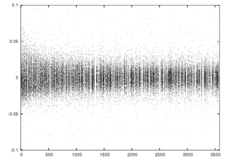
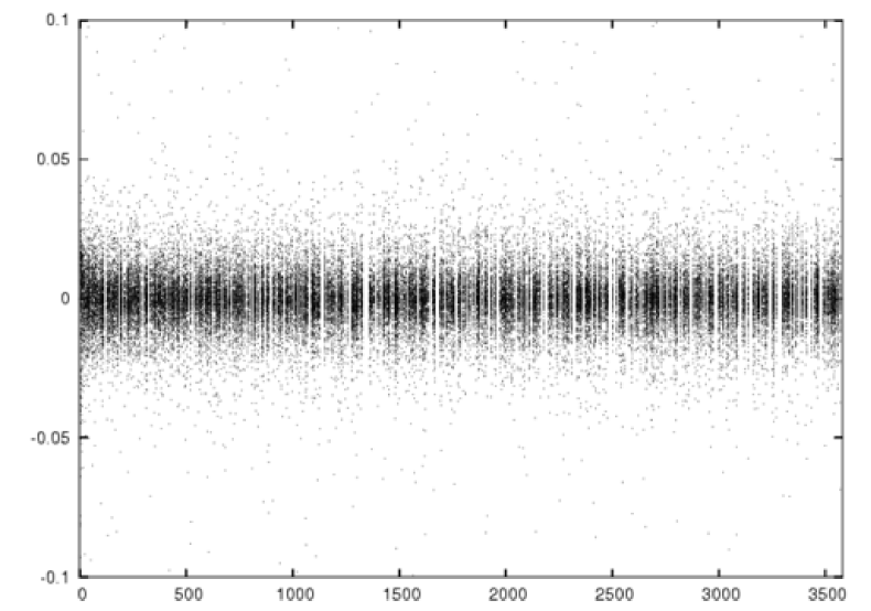
Figure 2: A plot for one hundred datasets of $R^{\pm}_{q}(10^{8})-R_{q}$, top plot, and of (64), bottom plot, for $2\leq q\leq 3571$.

Finally, a sequence of plots shows the dependence of the remainder term in the first and second order approximations on $q$ and $a_{q}$. Given an integer $n$, we display, in Figure 3 $q$ v.s. $R^{\pm}_{q}(10^{8})-R_{q}$ for the subset of our elliptic curves satisfying $a_{q}=n$. For each of $n=-20,-9,-6,-4,-3,-2,-1,0,1,2,3,4,6,9,20$ there is one plot. Figure 4 does the same but for the values given by equation (64).

We notice several things. Overall, the plots in the Figure 4 are more symmetric about the horizontal axis reflecting a tighter fit by including the second order term. For smaller $q$ however, incorporating the second order term leads to a correction that tends to overshoot. Compare for example the fourth plot in Figures 3 and 4. Presumably, the third and further order terms, while of size $O(\log(X)^{-2})$ can have relatively large constants for smaller $q$ requiring one to take $X$ larger than $10^{8}$ to see an improvement from the second order term.

This is also reflected in Tables 1– 2 which lists for two elliptic curves and the sets $S^{+}(10^{8})$ and $S^{-}(10^{8})$ the numeric values of (63) and (64) for $q\leq 179$.

Figure 3: Left to right, top to bottom: $n=-20,-9,-6,-4,-3,-2,-1,0,1,2,3,4,6,9,20$. Values of $R^{\pm}_{q}(X)-R_{q}$, with $X=10^{8}$, $2\leq q<500$, for the subset of our elliptic curves satisfying $a_{q}=n$. The blank white area on the left of the plots for larger $n$ reflects Hasse’s theorem that $|a_{q}|<2q^{1/2}$ which restricts how small $q$ can be given $a_{q}=n$.

Figure 4: Left to right, top to bottom: $n=-20,-9,-6,-4,-3,-2,-1,0,1,2,3,4,6,9,20$ Values of (64), with $X=10^{8}$, $2\leq q<500$, for the subset of our elliptic curves satisfying $a_{q}=n$.

$q$ $a_{q}$ (63), $R^{-}$ case (64), $R^{-}$ case (63), $R^{+}$ case (64), $R^{+}$ case 2 -2 -0.0770803072 -0.1058493733 -0.0586746787 -0.0877402111 3 -1 -0.0226715635 -0.0314020531 -0.0112745015 -0.0200944948 5 1 0.0039386614 0.0110670332 0.0036670414 0.0108679937 7 -2 -0.0086677613 -0.0320476479 0.0122162834 -0.0114052128 13 4 -0.0117312471 0.0114581936 -0.0109800729 0.0124435613 17 -2 0.0068671146 -0.0078374991 0.0156420190 0.0007858160 19 0 0.0018786796 0.0018786796 0.0017548761 0.0017548761 23 -1 0.0065085545 0.0007253864 0.0087254527 0.0028829043 29 0 0.0015867409 0.0015867409 0.0024574134 0.0024574134 31 7 -0.0203976628 0.0065021478 -0.0212844047 0.0058867043 37 3 -0.0076213530 0.0038881303 -0.0081586993 0.0034679279 41 -8 0.0293718254 -0.0104233512 0.0370003139 -0.0032097869 43 -6 0.0200767559 -0.0066399665 0.0230632720 -0.0039304770 47 8 -0.0166158276 0.0077120067 -0.0181946828 0.0063789626 53 -6 0.0175200151 -0.0048911726 0.0194053316 -0.0032378110 59 5 -0.0095451504 0.0043844494 -0.0127090647 0.0013621363 61 12 -0.0229944549 0.0068341556 -0.0279181705 0.0022108579 67 -7 0.0114509369 -0.0104875891 0.0227073168 0.0005417642 71 -3 0.0078736247 -0.0004772247 0.0051206275 -0.0033160932 73 4 -0.0037492048 0.0060879152 -0.0119406010 -0.0020032563 79 -10 0.0300180540 0.0013488112 0.0296738495 0.0007070253 83 -6 0.0142507227 -0.0012053860 0.0124985709 -0.0031170117 89 15 -0.0230738419 0.0057929377 -0.0246777538 0.0044799769 97 -7 0.0105905604 -0.0054712607 0.0154867447 -0.0007408496 101 2 -0.0037100582 0.0002953972 -0.0044847165 -0.0004383257 103 -16 0.0324024693 -0.0068711726 0.0357260869 -0.0039571170 107 18 -0.0228240764 0.0073200274 -0.0245602341 0.0058874808 109 10 -0.0097574184 0.0078543625 -0.0133419792 0.0044484844 113 9 -0.0120886539 0.0035056429 -0.0113667336 0.0043859550 127 8 -0.0093873089 0.0034881040 -0.0081483592 0.0048580252 131 -18 0.0320681832 -0.0038139100 0.0371594888 0.0009037228 137 -7 0.0117897817 -0.0002445226 0.0086451554 -0.0035131214 139 10 -0.0148514126 0.0000259176 -0.0112784046 0.0037500975 149 -10 0.0140952751 -0.0023344544 0.0172405748 0.0006412396 151 2 -0.0041170706 -0.0011557351 -0.0070016068 -0.0040099902 157 -7 0.0108322334 0.0000925632 0.0097641977 -0.0010860401 163 4 -0.0014750980 0.0040361356 -0.0066512858 -0.0010837710 167 -12 0.0171132732 -0.0010302790 0.0222297420 0.0038987403 173 -6 0.0054181738 -0.0030119338 0.0036566390 -0.0048601622 179 -15 0.0177416502 -0.0040658274 0.0261766468 0.0041434818

Table 1: The values of $R^{\pm}_{q}(10^{8})$, for the elliptic curve $11_{A}$ of conductor 11 given by $y^{2}+y=x^{3}-x^{2}-10x-20$, compared to the conjectured first order approximation (63) and second order approximation (64).

$q$ $a_{q}$ (63), $R^{-}$ case (64), $R^{-}$ case (63), $R^{+}$ case (64), $R^{+}$ case 2 0 0.0001964177 0.0001964177 0.0025336244 0.0025336244 3 0 -0.0007380207 -0.0007380207 -0.0025236647 -0.0025236647 5 4 -0.0128879806 0.0109510354 -0.0166316058 0.0072258354 7 0 -0.0048614428 -0.0048614428 -0.0014203548 -0.0014203548 11 3 -0.0076239866 0.0095824910 -0.0101221542 0.0070977143 13 6 -0.0212338218 0.0089386380 -0.0276990384 0.0024967032 17 -1 0.0033655021 -0.0029005302 0.0086797465 0.0024087738 19 -1 0.0055745934 -0.0003223680 0.0020465484 -0.0038550619 23 -2 0.0074744917 -0.0036255406 0.0079256468 -0.0031831583 29 0 0.0004190042 0.0004190042 -0.0010879108 -0.0010879108 31 4 -0.0108662407 0.0041956843 -0.0096223973 0.0054512748 37 3 -0.0067227670 0.0037940655 -0.0162107316 -0.0056856756 41 5 -0.0109118090 0.0049138186 -0.0164777387 -0.0006397725 43 -10 0.0406071465 -0.0060036473 0.0409949651 -0.0056532348 47 -6 0.0284021024 0.0057897746 0.0209827487 -0.0016475471 53 -10 0.0361234610 -0.0017568821 0.0423409405 0.0044303004 59 4 -0.0054935724 0.0048495607 -0.0148985734 -0.0045473511 61 -8 0.0227634479 -0.0025651538 0.0253866588 0.0000379053 67 -8 0.0217284008 -0.0016029354 0.0249365465 0.0015866634 71 -15 0.0398795640 -0.0080932079 0.0531538377 0.0051425339 73 2 -0.0003657281 0.0042519609 -0.0019954011 0.0026259102 79 -13 0.0270702549 -0.0087950276 0.0328555729 -0.0030383756 83 5 -0.0120289758 -0.0018576129 -0.0140337206 -0.0038544019 89 9 -0.0117002661 0.0050406278 -0.0159501141 0.0008038275 97 7 -0.0121449601 0.0003884458 -0.0126491435 -0.0001059465 101 10 -0.0162655200 0.0006799944 -0.0166873803 0.0002713400 103 11 -0.0154514081 0.0027879315 -0.0155096044 0.0027439391 107 -15 0.0298791131 -0.0020491232 0.0346054275 0.0026517125 109 -7 0.0131301691 -0.0001660211 0.0138662913 0.0005595788 113 14 -0.0219346950 -0.0006197951 -0.0199798581 0.0013516122 127 17 -0.0231978866 0.0002623636 -0.0235951007 -0.0001166344 131 -6 0.0075864820 -0.0020988314 0.0132703492 0.0035773840 137 -6 0.0049307893 -0.0044030816 0.0085067787 -0.0008344650 139 14 -0.0179638452 0.0005718014 -0.0220919830 -0.0035419036 149 19 -0.0184587534 0.0048182811 -0.0206858659 0.0026092450 151 -14 0.0157624561 -0.0057016072 0.0217272592 0.0002461455 157 -14 0.0258394912 0.0051129620 0.0236949594 0.0029519710 163 -8 0.0115026664 0.0005637031 0.0044174198 -0.0065301910 167 21 -0.0224356707 0.0011192167 -0.0284090909 -0.0048359139 173 -6 0.0056158047 -0.0020804090 0.0044893748 -0.0032129134 179 0 0.0018844544 0.0018844544 -0.0007004350 -0.0007004350

Table 2: The values of $R^{\pm}_{q}(10^{8})$, for the elliptic curve $307_{A}$ of conductor 307 given by $y^{2}+y=x^{3}-x-9$, compared to the conjectured first order approximation (63) and second order approximation (64).

Acknowledgements

We wish to thank the Newton Institute in Cambridge where some of this research was carried out. We also thank Gonzalo Tornaria and Fernando Rodriguez-Villegas who supplied us with a table of weight three halves forms that were used to compute the $L$-values studied in this paper.

References

• [1] C. Breuil, B. Conrad, F. Diamond, and R. Taylor, J. Amer. Math. Soc. 14:843–939, 2001, no. 4.
• [2] J.B. Conrey and D.W. Farmer, Mean values of $L$-functions and symmetry, Int. Math. Res. Notices, 17:883–908, 2000. arXiv:math.nt/9912107.
• [3] J.B. Conrey, D.W. Farmer, J.P. Keating, M.O. Rubinstein, and N.C. Snaith, Autocorrelation of random matrix polynomials, Comm. Math. Phys.:365–395, 2003, no. 3. arXiv:math-ph/02080077.
• [4] J.B. Conrey, D.W. Farmer, J.P. Keating, M.O. Rubinstein, and N.C. Snaith, Integral moments of ${L}$-functions, Proceedings of the London Mathematical Society, 91, 33–104. arXiv:math.nt/0206018.
• [5] J.B. Conrey, J.P. Keating, M.O. Rubinstein, and N.C. Snaith, On the frequency of vanishing of quadratic twists of modular ${L}$-functions, In Number Theory for the Millennium I: Proceedings of the Millennial Conference on Number Theory; editor, M.A. Bennett et al., pages 301–315. A K Peters, Ltd, Natick, 2002. arXiv:math.nt/0012043.
• [6] J.B. Conrey, J.P. Keating, M.O. Rubinstein, and N.C. Snaith, Random Matrix Theory and the Fourier Coefficients of Half-Integral Weight Forms, Experimental Mathematics, 15 2006, no. 1. arXiv:math.nt/0412083
• [7] C. Delaunay, Note on the frequency of vanishing of $L$-functions of elliptic curves in a family of quadratic twists, preprint.
• [8] J.P. Keating and N.C. Snaith, Random matrix theory and ${L}$-functions at $s=1/2$, Commun. Math. Phys, 214:91–110, 2000.
• [9] F. Rodriguez-Villegas and G. Tornaria, private communication.
• [10] M. Rubinstein, The $L$-function database, Available at www.math.uwaterloo.ca/$\sim$mrubinst.
• [11] R. Taylor and A. Wiles Ring-theoretic properties of certain Hecke algebras Ann. of Math., (2) 141:553–572 (1995), no. 3.
• [12] A. Wiles, Modular elliptic curves and Fermat’s last theorem, Ann. of Math., (2) 141:443–551 (1995), no. 3.
J.B. Conrey
American Institute of Mathematics
360 Portage Avenue
Palo Alto, CA 94306
USA
School of Mathematics
University of Bristol
Bristol BS8 1TW
UK
A. Pocharel
Department of Mathematics
Princeton University
Princeton, NJ 08544
USA
M.O. Rubinstein
Pure Mathematics
University of Waterloo
200 University Ave W
Waterloo, ON, Canada
N2L 3G1
M. Watkins
School of Mathematics
University of Bristol
Bristol BS8 1TW
UK