The Circuit Ideal of a Vector Configuration

Abstract.

The circuit ideal, ${I_{{\mathcal{C}}_{\mathcal{A}}}}$, of a configuration $\mathcal{A}=\{{\bf{a}}_{1},\ldots,{\bf{a}}_{n}\}\subset\mathbb{Z}^{d}$ is the ideal generated by the binomials ${{\bf{x}}}^{{\bf{c}}^{+}}-{{\bf{x}}}^{{\bf{c}}^{-}}\in{\bf{k}}[x_{1},\ldots,x_{n}]$ as ${\bf{c}}={\bf{c}}^{+}-{\bf{c}}^{-}\in\mathbb{Z}^{n}$ varies over the circuits of $\mathcal{A}$. This ideal is contained in the toric ideal, ${{I_{\mathcal{A}}}}$, of $\mathcal{A}$ which has numerous applications and is nontrivial to compute. Since circuits can be computed using linear algebra and the two ideals often coincide, it is worthwhile to understand when equality occurs.

In this paper we study ${I_{{\mathcal{C}}_{\mathcal{A}}}}$ in relation to ${{I_{\mathcal{A}}}}$ from various algebraic and combinatorial perspectives. We prove that the obstruction to equality of the ideals is the existence of certain polytopes. This result is based on a complete characterization of the standard pairs/associated primes of a monomial initial ideal of ${I_{{\mathcal{C}}_{\mathcal{A}}}}$ and their differences from those for the corresponding toric initial ideal. Eisenbud and Sturmfels proved that ${{I_{\mathcal{A}}}}$ is the unique minimal prime of ${I_{{\mathcal{C}}_{\mathcal{A}}}}$ and that the embedded primes of ${I_{{\mathcal{C}}_{\mathcal{A}}}}$ are indexed by certain faces of the cone spanned by $\mathcal{A}$. We provide a necessary condition for a particular face to index an embedded prime and a partial converse. Finally, we compare various polyhedral fans associated to ${{I_{\mathcal{A}}}}$ and ${I_{{\mathcal{C}}_{\mathcal{A}}}}$. The Gröbner fan of ${I_{{\mathcal{C}}_{\mathcal{A}}}}$ is shown to refine that of ${{I_{\mathcal{A}}}}$ when the codimension of the ideals is at most two.

1. Introduction

Throughout this paper, we fix an ordered vector configuration $\mathcal{A}=\{{\bf{a}}_{1},\ldots,{\bf{a}}_{n}\}\subset\mathbb{Z}^{d}$. Assume that the $d\times n$ integer matrix $A=[{\bf{a}}_{1}\,\ldots\,{\bf{a}}_{n}]$ whose columns are the elements of $\mathcal{A}$ has rank $d$. Let ${{\mathcal{L}_{\mathcal{A}}}}$ be the $(n-d)$-dimensional saturated lattice $\{{\bf{u}}\in\mathbb{Z}^{n}\,:\,A{\bf{u}}={\bf 0}\}$. We assume that ${{\mathcal{L}_{\mathcal{A}}}}\cap\mathbb{N}^{n}=\{{\bf 0}\}$.

The support of a vector ${\bf{u}}\in\mathbb{Z}^{n}$ is defined to be $\textup{supp}({\bf{u}}):=\{i\,:\,u_{i}\neq 0\}$ and ${\bf{u}}$ is primitive if the greatest common divisor of its components is one.

Definition 1.1.

A vector ${\bf{c}}\in{{\mathcal{L}_{\mathcal{A}}}}$ is a circuit of $\mathcal{A}$ if (1) ${\bf{c}}$ is a non-zero primitive vector and (2) there does not exist ${\bf{d}}\in{{\mathcal{L}_{\mathcal{A}}}}$ with $\textup{supp}({\bf{d}})\subsetneq\textup{supp}({\bf{c}})$.

Let $\mathcal{C}_{\mathcal{A}}$ denote the set of all circuits of $\mathcal{A}$. Write ${\bf{c}}={\bf{c}}^{+}-{\bf{c}}^{-}$ where $c^{+}_{j}=c_{j}$ if $c_{j}>0$ and $0$ otherwise, and $c^{-}_{j}=-c_{j}$ if $c_{j}<0$ and $0$ otherwise. Identify ${\bf{c}}\in\mathcal{C}_{\mathcal{A}}$ with the binomial ${\bf{x}}^{{\bf{c}}^{+}}-{\bf{x}}^{{\bf{c}}^{-}}\in{\bf{k}}[x_{1},\ldots,x_{n}]=:{\bf{k}}[{\bf{x}}]$ where ${\bf{k}}$ is an algebraically closed field and ${\bf{x}}^{\bf{u}}:=x_{1}^{u_{1}}x_{2}^{u_{2}}\cdots x_{n}^{u_{n}}$. We refer to both ${\bf{c}}$ and ${\bf{x}}^{{\bf{c}}^{+}}-{\bf{x}}^{{\bf{c}}^{-}}$ as a circuit of $\mathcal{A}$ and denote both lists by $\mathcal{C}_{\mathcal{A}}$.

Definition 1.2.

The circuit ideal of $\mathcal{A}$ is the binomial ideal ${I_{{\mathcal{C}}_{\mathcal{A}}}}:=\langle\mathcal{C}_{\mathcal{A}}\rangle\subseteq{\bf{k}}[{\bf{x}}].$

The circuit ideal ${I_{{\mathcal{C}}_{\mathcal{A}}}}$ is a subideal of the binomial prime toric ideal of $\mathcal{A}$

$${{I_{\mathcal{A}}}}:=\langle{\bf{x}}^{{\bf{u}}^{+}}-{\bf{x}}^{{\bf{u}}^{-}}\,:\,{\bf{u}}\in{{\mathcal{L}_{\mathcal{A}}}}\rangle.$$

Toric ideals are the defining ideals of toric varieties [8] and have numerous applications in combinatorics, optimization, algebra and algebraic geometry [18]. These connections make the computability of ${{I_{\mathcal{A}}}}$ an important practical concern.

Proposition 1.3.

[18] Given a finite subset ${\mathcal{B}}$ of ${{\mathcal{L}_{\mathcal{A}}}}$, define the ideal $J_{{\mathcal{B}}}:=\langle{\bf{x}}^{{\bf{b}}^{+}}-{\bf{x}}^{{\bf{b}}^{-}}\,:\,{\bf{b}}\in{\mathcal{B}}\rangle\subset{\bf{k}}[{\bf{x}}]$. A set ${\mathcal{B}}$ spans ${{\mathcal{L}_{\mathcal{A}}}}$ if and only if $(J_{{\mathcal{B}}}\,:\,(x_{1}x_{2}\cdots x_{n})^{\infty})={{I_{\mathcal{A}}}}$.

Proposition 1.3 is the starting point of the best algorithms to compute ${{I_{\mathcal{A}}}}$ since a spanning set ${\mathcal{B}}$ of ${{\mathcal{L}_{\mathcal{A}}}}$ can be computed easily and each saturation in

$$(J_{{\mathcal{B}}}\,:\,(x_{1}x_{2}\cdots x_{n})^{\infty})=((((J_{{\mathcal{B}}}\,:\,x_{1}^{\infty})\,:\,x_{2}^{\infty})\cdots)\,:\,x_{n}^{\infty})$$

can be achieved by a Gröbner basis calculation ([10], [18, Chapter 12].) It can be checked that ${\mathcal{C}}_{\mathcal{A}}$ spans ${{\mathcal{L}_{\mathcal{A}}}}$ and hence ${{I_{\mathcal{A}}}}=({I_{{\mathcal{C}}_{\mathcal{A}}}}\,:\,(x_{1}x_{2}\cdots x_{n})^{\infty})$. In many examples, ${I_{{\mathcal{C}}_{\mathcal{A}}}}$ equals ${{I_{\mathcal{A}}}}$, and since the circuits of a matrix can be computed easily [4, page 190], it is of interest to know how close the circuit ideal is to the toric ideal and in particular when they are equal. This raises the main problem addressed in this paper. See Remark 2.3 for further motivations.

Problem 1.4.

When does the circuit ideal ${I_{{\mathcal{C}}_{\mathcal{A}}}}$ equal the toric ideal ${{I_{\mathcal{A}}}}$?

In this paper, we investigate Problem 1.4 from several different angles. Let ${{\mathbb{N}A}}$ denote the semigroup $\{A{\bf{u}}\,:\,{\bf{u}}\in\mathbb{N}^{n}\}\subset\mathbb{Z}^{d}$. Both ${{I_{\mathcal{A}}}}$ and ${I_{{\mathcal{C}}_{\mathcal{A}}}}$ are homogeneous under multi-grading by ${{\mathbb{N}A}}$ with ${\bf{k}}[{\bf{x}}]/{{I_{\mathcal{A}}}}$ having Hilbert function value one for all ${\bf{b}}\in{{\mathbb{N}A}}$. In Section 2 we recall conditions for the equality of ${{I_{\mathcal{A}}}}$ and ${I_{{\mathcal{C}}_{\mathcal{A}}}}$ and then exhibit various properties of circuit ideals that contrast those of toric ideals. We interpret the multi-graded Hilbert function values of ${\bf{k}}[{\bf{x}}]/{I_{{\mathcal{C}}_{\mathcal{A}}}}$.

From the point of view of Gröbner basis theory, it is natural to investigate ${{I_{\mathcal{A}}}}$ and ${I_{{\mathcal{C}}_{\mathcal{A}}}}$ by examining the difference between their initial ideals with respect to a fixed weight vector $\omega$. In Section 3, we give a complete characterization of the associated primes of a monomial initial ideal of ${I_{{\mathcal{C}}_{\mathcal{A}}}}$ (Theorem 3.11) extending previously known characterizations of the associated primes of a monomial initial ideal of ${{I_{\mathcal{A}}}}$ [11]. The associated primes and the difference between the two monomial initial ideals are described in terms of certain polytopes that depend on $\mathcal{A}$ and $\omega$. Using this we answer Problem 1.4 by showing that the obstruction to equality of the ideals is the existence of certain polytopes of the above type (Theorem 3.21).

In [6], Eisenbud and Sturmfels showed that ${{I_{\mathcal{A}}}}$ is the unique minimal prime of ${I_{{\mathcal{C}}_{\mathcal{A}}}}$. Thus a second natural measure of the difference between the two ideals is an understanding of the embedded primes of ${I_{{\mathcal{C}}_{\mathcal{A}}}}$. Let $\textup{cone}(\mathcal{A})$ denote the $d$-dimensional cone spanned by $\mathcal{A}$. Record a face $\sigma$ of $\textup{cone}(\mathcal{A})$ as the set of indices, $j$, of all ${\bf{a}}_{j}$ that lie on $\sigma$. Eisenbud and Sturmfels proved that the associated primes of ${I_{{\mathcal{C}}_{\mathcal{A}}}}$ are all of the form $P_{\sigma}+{{I_{\mathcal{A}}}}$ where $\sigma$ is some face of $\textup{cone}(\mathcal{A})$ and $P_{\sigma}:=\langle x_{j}\,:\,j\not\in\sigma\rangle$. In particular, ${{I_{\mathcal{A}}}}=P_{[n]}+{{I_{\mathcal{A}}}}$ is indexed by the full face $[n]:=\{1,2,\ldots,n\}$ of $\textup{cone}(\mathcal{A})$. However, not all faces of $\textup{cone}(\mathcal{A})$ need index an associated prime of ${I_{{\mathcal{C}}_{\mathcal{A}}}}$ and Eisenbud and Sturmfels raise the following problem.

Problem 1.5.

[6, §7] “It remains an interesting combinatorial problem to characterize the embedded primary components of the circuit ideal ${I_{{\mathcal{C}}_{\mathcal{A}}}}$. In particular, which faces of $\textup{cone}(\mathcal{A})$ support an associated prime of ${I_{{\mathcal{C}}_{\mathcal{A}}}}$? An answer to this question might be valuable for the applications of binomial ideals to integer programming and statistics.”

In Section 4, we give a necessary condition for a prime $P_{\sigma}+{{I_{\mathcal{A}}}}$ to be an embedded prime of ${I_{{\mathcal{C}}_{\mathcal{A}}}}$ (Theorem 4.4) using the results in Section 3. We also provide a partial converse to Theorem 4.4. As an application, we derive connections between the smoothness of the toric variety defined by a face $\sigma$ of $\textup{cone}(\mathcal{A})$ and $P_{\sigma}+{{I_{\mathcal{A}}}}$ being an embedded prime of ${I_{{\mathcal{C}}_{\mathcal{A}}}}$ when $\mathcal{A}$ is a graded vector configuration.

We conclude the paper in Section 5 by examining various polyhedral fans associated to ${{I_{\mathcal{A}}}}$ and ${I_{{\mathcal{C}}_{\mathcal{A}}}}$. Given a homogeneous ideal $I$ and a weight vector $\omega\in\mathbb{R}^{n}$, let $\textup{in}_{\omega}(I)$ be the initial ideal of $I$ with respect to $\omega$, $\sqrt{\textup{in}_{\omega}(I)}$ the radical of $\textup{in}_{\omega}(I)$, and $\textup{top}(\textup{in}_{\omega}(I))$ the intersection of the top-dimensional primary components of $\textup{in}_{\omega}(I)$. These entities define three equivalence relations on $\mathbb{R}^{n}$ as follows.

1. The initial ideal equivalence relation: ${\bf{u}}\sim{\bf{v}}\Leftrightarrow\textup{in}_{{\bf{u}}}(I)=\textup{in}_{{\bf{v}}}(I)$,

2. the top equivalence relation: ${\bf{u}}\sim{\bf{v}}\Leftrightarrow\textup{top}(\textup{in}_{{\bf{u}}}(I))=\textup{top}(\textup{in}_{{\bf{v}}}(I))$, and

3. the radical equivalence relation: ${\bf{u}}\sim{\bf{v}}\Leftrightarrow\sqrt{\textup{in}_{{\bf{u}}}(I)}=\sqrt{\textup{in}_{{\bf{v}}}(I)}$.

For any homogeneous ideal $I$, the initial ideal equivalence classes form the cells of the Gröbner fan of $I$ [14], [18, Chapter 2]. For ${{I_{\mathcal{A}}}}$ it is well known that the other two equivalence classes also form polyhedral fans — the radical equivalence relation gives the secondary fan of $\mathcal{A}$ [2], [18, Chapter 8], and the top equivalence relation gives the hypergeometric fan of $\mathcal{A}$ [16]. We prove that for ${I_{{\mathcal{C}}_{\mathcal{A}}}}$, the top dimensional equivalence classes of the radical and top equivalence relations coincide with those for ${{I_{\mathcal{A}}}}$ (Theorem 5.16 and Proposition 5.19). However, the Gröbner fans of ${{I_{\mathcal{A}}}}$ and ${I_{{\mathcal{C}}_{\mathcal{A}}}}$ do not coincide in general. Corollary 5.21 proves that when the codimension of the ideals is at most two, the Gröbner fan of ${I_{{\mathcal{C}}_{\mathcal{A}}}}$ refines that of ${{I_{\mathcal{A}}}}$.

2. Properties of ${{I_{\mathcal{A}}}}$ versus ${I_{{\mathcal{C}}_{\mathcal{A}}}}$

In this section we first collect conditions equivalent to the equality of ${{I_{\mathcal{A}}}}$ and ${I_{{\mathcal{C}}_{\mathcal{A}}}}$. Many of these stem from combinatorics and optimization and most are well known [4], [18]. We then contrast ${I_{{\mathcal{C}}_{\mathcal{A}}}}$ with ${{I_{\mathcal{A}}}}$ in light of these conditions.

Consider the semigroup homomorphism $\pi:\,\mathbb{N}^{n}\rightarrow{{\mathbb{N}A}}\,,\;{\bf{u}}\mapsto A{\bf{u}}$. Both ${{I_{\mathcal{A}}}}$ and ${I_{{\mathcal{C}}_{\mathcal{A}}}}$ are homogeneous under the $\mathcal{A}$-grading of ${\bf{k}}[{\bf{x}}]$ by $\textup{deg}(x_{i})={\bf{a}}_{i}$ for $i=1,\ldots,n$ since every binomial of the form ${\bf{x}}^{\bf{u}}-{\bf{x}}^{\bf{v}}$ in either ideal is $\mathcal{A}$-homogeneous with $\mathcal{A}$-degree $\pi({\bf{u}})=A{\bf{u}}=A{\bf{v}}=\pi({\bf{v}})$. Let ${{\mathbf{H}_{{I_{{\mathcal{C}}_{\mathcal{A}}}}}}}\,:\,{{\mathbb{N}A}}\rightarrow\mathbb{N}$ be the $\mathcal{A}$-graded Hilbert function of ${\bf{k}}[{\bf{x}}]/{I_{{\mathcal{C}}_{\mathcal{A}}}}$ given by ${\bf{b}}\mapsto\dim_{{\bf{k}}}({\bf{k}}[{\bf{x}}]/{I_{{\mathcal{C}}_{\mathcal{A}}}})_{{\bf{b}}}$. Let ${{\mathbf{H}_{{{I_{\mathcal{A}}}}}}}$ be the same for ${{I_{\mathcal{A}}}}$.

Since ${{\mathcal{L}_{\mathcal{A}}}}\cap\mathbb{N}^{n}=\{{\bf 0}\}$, for each ${\bf{b}}\in{{\mathbb{N}A}}$, the polyhedron $P_{{\bf{b}}}:=\{{\bf{x}}\in\mathbb{R}^{n}_{\geq 0}\,:\,A{\bf{x}}={\bf{b}}\}$ is bounded [17] which implies that $\pi^{-1}({\bf{b}}):=\{{\bf{x}}\in\mathbb{N}^{n}\,:\,A{\bf{x}}={\bf{b}}\}=P_{{\bf{b}}}\cap\mathbb{N}^{n}$ is finite for all ${\bf{b}}\in{{\mathbb{N}A}}$. For a fixed ${\bf{b}}\in{{\mathbb{N}A}}$, the vertex set $\pi^{-1}({\bf{b}})$ admits four natural graphs as follows. First, choose binomial generating sets $G({{I_{\mathcal{A}}}})$ and $G({I_{{\mathcal{C}}_{\mathcal{A}}}})$ of ${{I_{\mathcal{A}}}}$ and ${I_{{\mathcal{C}}_{\mathcal{A}}}}$ respectively, and let $\mathcal{F}({\bf{b}})$ and $\mathcal{F}^{\mathcal{C}}({\bf{b}})$ be graphs on $\pi^{-1}({\bf{b}})$ such that ${\bf{u}}$ is adjacent to ${\bf{v}}$ in $\mathcal{F}({\bf{b}})$ (respectively in $\mathcal{F}^{\mathcal{C}}({\bf{b}})$) if ${\bf{x}}^{\bf{u}}-{\bf{x}}^{\bf{v}}$ is a monomial multiple of a binomial in $G({{I_{\mathcal{A}}}})$ (respectively in $G({I_{{\mathcal{C}}_{\mathcal{A}}}})$). Next, fix a generic weight vector $\omega\in\mathbb{R}^{n}$ in the sense that the initial ideals $\textup{in}_{\omega}({{I_{\mathcal{A}}}})$ and $\textup{in}_{\omega}({I_{{\mathcal{C}}_{\mathcal{A}}}})$ are both monomial ideals. Let $G_{\omega}({{I_{\mathcal{A}}}})$ and $G_{\omega}({I_{{\mathcal{C}}_{\mathcal{A}}}})$ be the marked reduced Gröbner bases of ${{I_{\mathcal{A}}}}$ and ${I_{{\mathcal{C}}_{\mathcal{A}}}}$ with respect to $\omega$. Elements of these Gröbner bases are $\mathcal{A}$-homogeneous binomials and the Gröbner basis being marked means that the first term in each binomial $f$ is its initial term $\textup{in}_{\omega}(f)$. Construct the directed graphs $\mathcal{F}_{\omega}({\bf{b}})$ and $\mathcal{F}^{\mathcal{C}}_{\omega}({\bf{b}})$ on $\pi^{-1}({\bf{b}})$ by drawing an arrow from ${\bf{u}}$ to ${\bf{v}}$ in $\mathcal{F}_{\omega}({\bf{b}})$ (respectively $F^{\mathcal{C}}_{\omega}({\bf{b}})$) if and only if ${\bf{x}}^{{\bf{u}}}-{\bf{x}}^{{\bf{v}}}$ is a monomial multiple of some marked binomial in $G_{\omega}({{I_{\mathcal{A}}}})$ (respectively $G_{\omega}({I_{{\mathcal{C}}_{\mathcal{A}}}})$).

Lemma 2.1.

[4, Theorem 1.1] Vectors ${\bf{u}},{\bf{v}}\in\pi^{-1}({\bf{b}})$ are in the same component of $\mathcal{F}({\bf{b}})$ (respectively $\mathcal{F}^{\mathcal{C}}({\bf{b}})$) if and only if ${\bf{x}}^{{\bf{u}}}-{\bf{x}}^{{\bf{v}}}$ lies in ${{I_{\mathcal{A}}}}$ (respectively ${I_{{\mathcal{C}}_{\mathcal{A}}}}$).

Lemma 2.1 shows that while the edges in $\mathcal{F}({\bf{b}})$ and $\mathcal{F}^{\mathcal{C}}({\bf{b}})$ depend on the choice of generating sets $G({{I_{\mathcal{A}}}})$ and $G({I_{{\mathcal{C}}_{\mathcal{A}}}})$, the components, and in particular the number of components, do not depend on this choice. Further, both $\mathcal{F}({\bf{b}})$ and $\mathcal{F}_{\omega}({\bf{b}})$ partition $\pi^{-1}({\bf{b}})$ identically into components. The same holds for $\mathcal{F}^{\mathcal{C}}({\bf{b}})$ and $\mathcal{F}_{\omega}^{\mathcal{C}}({\bf{b}})$. The following theorem mostly collects results from [4] and [18].

Theorem 2.2.

The following statements are equivalent.

1. The ideals ${{I_{\mathcal{A}}}}$ and ${I_{{\mathcal{C}}_{\mathcal{A}}}}$ are equal.

2. For every ${\bf{b}}\in{{\mathbb{N}A}}$, the graph $\mathcal{F}^{\mathcal{C}}({\bf{b}})$ is connected.

3. For every ${\bf{b}}\in{{\mathbb{N}A}}$, the digraph $\mathcal{F}^{\mathcal{C}}_{\omega}({\bf{b}})$ has a unique sink. (In this case, the unique sink ${\bf{u}}$ in $\mathcal{F}^{\mathcal{C}}_{\omega}({\bf{b}})$ is the optimal solution of the integer program $\textup{minimize}\,\{\omega\cdot{\bf{x}}\,:\,A{\bf{x}}={\bf{b}},\,{\bf{x}}\in\mathbb{N}^{n}\}$.)

4. For every ${\bf{b}}\in{{\mathbb{N}A}}$ and generic weight vector $\omega\in\mathbb{R}^{n}$, $\textup{in}_{\omega}({I_{{\mathcal{C}}_{\mathcal{A}}}})$ has a unique standard monomial of $\mathcal{A}$-degree ${\bf{b}}$. (In this case, the standard monomial of $\mathcal{A}$-degree ${\bf{b}}$ is ${\bf{x}}^{\bf{u}}$ where ${\bf{u}}$ is the unique sink in $\mathcal{F}^{\mathcal{C}}_{\omega}({\bf{b}})$.)

5. For every ${\bf{b}}\in{{\mathbb{N}A}}$, the Hilbert function value ${{\mathbf{H}_{{I_{{\mathcal{C}}_{\mathcal{A}}}}}}}({\bf{b}})$ is one.

Proof:   Statements (2)–(5) are all true if ${I_{{\mathcal{C}}_{\mathcal{A}}}}$ is replaced by ${{I_{\mathcal{A}}}}$, $\mathcal{F}^{\mathcal{C}}({\bf{b}})$ by $\mathcal{F}({\bf{b}})$ and $\mathcal{F}^{\mathcal{C}}_{\omega}({\bf{b}})$ by $\mathcal{F}_{\omega}({\bf{b}})$, see [18, Chapters 4,5,10]. Further, ${{I_{\mathcal{A}}}}={I_{{\mathcal{C}}_{\mathcal{A}}}}$ if and only if $G_{\omega}({{I_{\mathcal{A}}}})=G_{\omega}({I_{{\mathcal{C}}_{\mathcal{A}}}})$ if and only if for each ${\bf{b}}$, $\mathcal{F}^{\mathcal{C}}_{\omega}({\bf{b}})$ equals $\mathcal{F}_{\omega}({\bf{b}})$ and hence if and only if $\mathcal{F}^{\mathcal{C}}({\bf{b}})$ and $\mathcal{F}({\bf{b}})$ have the same components. Hence (1) is equivalent to (2) and (3). Since ${I_{{\mathcal{C}}_{\mathcal{A}}}}\subseteq{{I_{\mathcal{A}}}}$, the two ideals are equal if and only if (5). The equivalence of (3) and (4) follows from Lemma 2.5 below. $\square$

Remark 2.3.

1. The connectivity of $\mathcal{F}({\bf{b}})$ was used in [5], in the context of statistical sampling, to devise random walks on $\pi^{-1}({\bf{b}})$. The equality of ${{I_{\mathcal{A}}}}$ and ${I_{{\mathcal{C}}_{\mathcal{A}}}}$ allows $\pi^{-1}({\bf{b}})$ to be connected using $G({I_{{\mathcal{C}}_{\mathcal{A}}}})$, which is cheaper to compute than $G({{I_{\mathcal{A}}}})$. In Section 3 we will see that for most ${\bf{b}}\in{{\mathbb{N}A}}$, $\mathcal{F}^{\mathcal{C}}({\bf{b}})$ is in fact connected (Theorem 3.16), and that the set of ${\bf{b}}\in{{\mathbb{N}A}}$ for which $\mathcal{F}^{\mathcal{C}}({\bf{b}})$ is disconnected can be described precisely. See also [4].

2. The equality of ${{I_{\mathcal{A}}}}$ and ${I_{{\mathcal{C}}_{\mathcal{A}}}}$ will allow all integer programs of the form

   $$\textup{minimize}\,\{\omega\cdot{\bf{x}}\,:\,A{\bf{x}}={\bf{b}},{\bf{x}}\in\mathbb{N}^{n}\}$$

   as ${\bf{b}}$ and $\omega$ vary to be solved by reduced Gröbner bases of ${I_{{\mathcal{C}}_{\mathcal{A}}}}$. The significance of this is that the circuits of $\mathcal{A}$ are precisely the primitive edge directions of the polyhedra $P_{{\bf{b}}}$ as ${\bf{b}}$ varies in ${{\mathbb{N}A}}$ and hence the directions taken by the simplex algorithm in solving linear programs of the form

   $$\textup{minimize}\,\{\omega\cdot{\bf{x}}\,:\,A{\bf{x}}={\bf{b}},{\bf{x}}\in\mathbb{R}^{n}_{\geq 0}\}$$

   as ${\bf{b}}$ and $\omega$ vary. Hence, even though ${I_{{\mathcal{C}}_{\mathcal{A}}}}$ contains more than the circuits of $\mathcal{A}$, philosophically, the equality of ${{I_{\mathcal{A}}}}$ and ${I_{{\mathcal{C}}_{\mathcal{A}}}}$ allows integer programs arising from $A$ to be solved via the corresponding linear programming data.

We now exhibit various properties of ${I_{{\mathcal{C}}_{\mathcal{A}}}}$ that contrast those of ${{I_{\mathcal{A}}}}$.

Proposition 2.4.

1. The graph $\mathcal{F}^{\mathcal{C}}({\bf{b}})$ may have arbitrarily many components, even if we restrict to the case of $A\in\mathbb{Z}^{1\times 3}$.

2. The standard monomials of $\textup{in}_{\omega}({I_{{\mathcal{C}}_{\mathcal{A}}}})$ of $\mathcal{A}$-degree ${\bf{b}}$ are not necessarily the cheapest monomials of that degree with respect to $\omega$.

Proof:   (1) For any natural number $k\geq 2$, take $A_{k}=\left(\begin{array}[]{rrr}k&2k+1&3k+1\end{array}\right).$ Since the three entries are pairwise relatively prime, the circuits are $x^{2k+1}-y^{k}$, $x^{3k+1}-z^{k}$, and $y^{3k+1}-z^{2k+1}$. Their respective $\mathcal{A}$-degrees are $2k^{2}+k,3k^{2}+k$, and $6k^{2}+5k+1$. Thus the graph $\mathcal{F}^{\mathcal{C}}(b)$ has no edges when $b<2k^{2}+k$. In particular, this holds if we take $b=m(3k+1)$ for $m=\lfloor k/2\rfloor$. This graph has at least $m+1$ vertices $\{(j,j,m-j):0\leq j\leq m\}$, so it has at least $m+1=\lfloor k/2\rfloor+1$ components.

(2) Consider $\mathcal{A}=\{3,4,5\}$. The graded reverse lexicographic (grevlex) Gröbner basis of ${I_{{\mathcal{C}}_{\mathcal{A}}}}$ with $a\succ b\succ c$ is

$$\{a^{4}-b^{3},ab^{3}-c^{3},b^{5}-c^{4},b^{2}c^{3}-ac^{4},a^{3}c^{3}-bc^{4},a^{2}bc^{4}-c^{6}\}.$$

The monomials of degree $17$ are $a^{4}c,a^{3}b^{2},abc^{2}$ and $b^{3}c$ of which the last three are standard monomials of the above grevlex initial ideal of ${I_{{\mathcal{C}}_{\mathcal{A}}}}$. However, we see that the non-standard monomial $a^{4}c$ is cheaper than the standard monomial $a^{3}b^{2}$. $\square$

We now prove that ${{\mathbf{H}_{{I_{{\mathcal{C}}_{\mathcal{A}}}}}}}({\bf{b}})$ equals the number of components of $\mathcal{F}^{\mathcal{C}}_{\omega}({\bf{b}})$, or equivalently, $\mathcal{F}^{\mathcal{C}}({\bf{b}})$. Proposition 2.4 (1) then shows that the values of ${{\mathbf{H}_{{I_{{\mathcal{C}}_{\mathcal{A}}}}}}}$ can be arbitrarily large even for $d$ and $n$ fixed. In contrast, ${{\mathbf{H}_{{{I_{\mathcal{A}}}}}}}({\bf{b}})=1$ for all ${\bf{b}}\in{{\mathbb{N}A}}$.

Lemma 2.5.

1. Let ${\bf{x}}^{{\bf{u}}}$ be a standard monomial of $\textup{in}_{\omega}({I_{{\mathcal{C}}_{\mathcal{A}}}})$ with $A{\bf{u}}={\bf{b}}$. Then for all ${\bf{v}}\neq{\bf{u}}$ in the same component of $\mathcal{F}^{\mathcal{C}}_{\omega}({\bf{b}})$ as ${\bf{u}}$, $\omega\cdot{\bf{u}}<\omega\cdot{\bf{v}}$. In particular, if ${\bf{p}}\in\mathbb{N}^{n}$, $A{\bf{p}}={\bf{b}}$, and $\omega\cdot{\bf{p}}<\omega\cdot{\bf{u}}$, then ${\bf{x}}^{{\bf{u}}}-{\bf{x}}^{{\bf{p}}}\not\in{I_{{\mathcal{C}}_{\mathcal{A}}}}$.

2. Each component of $\mathcal{F}^{\mathcal{C}}_{\omega}({\bf{b}})$ has a unique sink ${\bf{u}}$ and ${\bf{x}}^{{\bf{u}}}$ is the unique standard monomial of $\textup{in}_{\omega}({I_{{\mathcal{C}}_{\mathcal{A}}}})$ among all monomials ${\bf{x}}^{{\bf{v}}}$ such that ${\bf{v}}$ is in the same component as ${\bf{u}}$.

Proof:   (1) If ${\bf{v}}\,(\neq{\bf{u}})$ lies in the same component of $\mathcal{F}^{\mathcal{C}}_{\omega}({\bf{b}})$ as ${\bf{u}}$, then by Lemma 2.1, $0\neq f:={\bf{x}}^{{\bf{v}}}-{\bf{x}}^{{\bf{u}}}\in{I_{{\mathcal{C}}_{\mathcal{A}}}}$. Since ${\bf{x}}^{{\bf{u}}}\not\in\textup{in}_{\omega}({I_{{\mathcal{C}}_{\mathcal{A}}}})$, $\textup{in}_{\omega}(f)$ equals either ${\bf{x}}^{\bf{v}}$ or $f$. By the genericity of $\omega$, we can assume $\textup{in}_{\omega}(f)\neq f$. Thus $\omega\cdot{\bf{u}}<\omega\cdot{\bf{v}}$.

(2) Let $D$ be an arbitrary component of $\mathcal{F}^{\mathcal{C}}_{\omega}({\bf{b}})$, ${\bf{v}}$ be an arbitrary vertex in $D$, and ${\bf{x}}^{{\bf{u}}}$ be the normal form of ${\bf{x}}^{{\bf{v}}}$ with respect to $G_{\omega}({I_{{\mathcal{C}}_{\mathcal{A}}}})$. Then ${\bf{x}}^{{\bf{u}}}$ is a standard monomial of $\textup{in}_{\omega}({I_{{\mathcal{C}}_{\mathcal{A}}}})$ and by Lemma 2.1, ${\bf{u}}$ is in $D$. If ${\bf{x}}^{{\bf{u}}^{\prime}}$ is another standard monomial of $\textup{in}_{\omega}({I_{{\mathcal{C}}_{\mathcal{A}}}})$ with ${\bf{u}}^{\prime}$ in $D$, then by Lemma 2.1, $f:={\bf{x}}^{\bf{u}}-{\bf{x}}^{{\bf{u}}^{\prime}}\in{I_{{\mathcal{C}}_{\mathcal{A}}}}$ with $\textup{in}_{\omega}(f)$ equal to either ${\bf{x}}^{\bf{u}}$ or ${\bf{x}}^{{\bf{u}}^{\prime}}$, a contradiction. This implies that ${\bf{x}}^{\bf{u}}$ is the unique normal form of all ${\bf{x}}^{\bf{v}}$, ${\bf{v}}\in D$ and hence it is the unique sink in $D$. $\square$

Proposition 2.6.

The Hilbert function value ${{\mathbf{H}_{{I_{{\mathcal{C}}_{\mathcal{A}}}}}}}({\bf{b}})$ equals the number of components of $\mathcal{F}^{\mathcal{C}}_{\omega}({\bf{b}})$.

Proof:   By Lemma 2.5 (2), each component of $\mathcal{F}^{\mathcal{C}}_{\omega}({\bf{b}})$ contributes precisely one standard monomial of $\textup{in}_{\omega}({I_{{\mathcal{C}}_{\mathcal{A}}}})$. The number of standard monomials of $\textup{in}_{\omega}({I_{{\mathcal{C}}_{\mathcal{A}}}})$ of degree ${\bf{b}}$ equals $\dim_{{\bf{k}}}({\bf{k}}[{\bf{x}}]/\textup{in}_{\omega}({I_{{\mathcal{C}}_{\mathcal{A}}}}))_{{\bf{b}}}=\dim_{{\bf{k}}}({\bf{k}}[{\bf{x}}]/{I_{{\mathcal{C}}_{\mathcal{A}}}})_{{\bf{b}}}={{\mathbf{H}_{{I_{{\mathcal{C}}_{\mathcal{A}}}}}}}({\bf{b}})$. $\square$

Example 2.7.

When ${{I_{\mathcal{A}}}}\neq{I_{{\mathcal{C}}_{\mathcal{A}}}}$, the distribution of values of ${{\mathbf{H}_{{I_{{\mathcal{C}}_{\mathcal{A}}}}}}}$ can be quite complicated. In Figure 1, we plot these values for the matrix

$$A=\left(\begin{array}[]{rrrr}1&3&2&4\\ 1&4&5&2\end{array}\right).$$

The boundary of $\textup{cone}(\mathcal{A})$ is shown by dashed lines. Notice that deep in the interior of the cone, all of the values are one. Theorem 3.16 proves this fact.

Figure 1. The distribution of values of ${{\mathbf{H}_{{I_{{\mathcal{C}}_{\mathcal{A}}}}}}}$ for the matrix $A$ in Example 2.7.

3. Monomial Initial Ideals of the Circuit Ideal

Fix a generic weight vector $\omega\in\mathbb{R}^{n}$ such that $\textup{in}_{\omega}({{I_{\mathcal{A}}}})$ and $\textup{in}_{\omega}({I_{{\mathcal{C}}_{\mathcal{A}}}})$ are both monomial ideals. The main result of this section is Theorem 3.11 which characterizes the associated primes of $\textup{in}_{\omega}({I_{{\mathcal{C}}_{\mathcal{A}}}})$ in terms of certain polytopes defined from $\mathcal{A}$ and $\omega$ and their lattice points. This theorem generalizes Theorem 2.5 in [11] which gave a complete characterization of the associated primes of $\textup{in}_{\omega}({{I_{\mathcal{A}}}})$ in terms of certain lattice-point-free polytopes defined from $\mathcal{A}$ and $\omega$. Using Theorem 3.11, we describe the similarities and differences between the associated primes (standard pairs) of $\textup{in}_{\omega}({{I_{\mathcal{A}}}})$ and $\textup{in}_{\omega}({I_{{\mathcal{C}}_{\mathcal{A}}}})$, and give an answer to Problem 1.4 (Theorem 3.21).

To begin, we prove that $\textup{in}_{\omega}({{I_{\mathcal{A}}}})$ and $\textup{in}_{\omega}({I_{{\mathcal{C}}_{\mathcal{A}}}})$ have the same radical. This result was stated in [15] without proof. If ${\bf{u}}$ and ${\bf{v}}$ are vectors in $\mathbb{Z}^{n}$, then we say that ${\bf{u}}$ is conformal to ${\bf{v}}$ if $\textup{supp}({\bf{u}}^{+})\subseteq\textup{supp}({\bf{v}}^{+})$ and $\textup{supp}({\bf{u}}^{-})\subseteq\textup{supp}({\bf{v}}^{-})$. Lemma 4.10 in [18] states that every vector ${\bf{v}}\in{{\mathcal{L}_{\mathcal{A}}}}$ can be written as a non-negative rational combination of $n-d$ circuits of $\mathcal{A}$ that are conformal to ${\bf{v}}$.

Lemma 3.1.

If ${\bf{x}}^{\alpha}-{\bf{x}}^{\beta}\in{{I_{\mathcal{A}}}}$ then there exists $s\in\mathbb{N}_{>0}$ such that ${\bf{x}}^{s\alpha}-{\bf{x}}^{s\beta}\in{I_{{\mathcal{C}}_{\mathcal{A}}}}$.

Proof:   Suppose $\textup{supp}(\alpha)\cap\textup{supp}(\beta)=\emptyset$. By [18, Lemma 4.10], $\alpha-\beta=\sum_{i=1}^{t}q_{i}{\bf{c}}_{i}$ where ${\bf{c}}_{i}$ are circuits of $\mathcal{A}$ conformal to $\alpha-\beta$ and $q_{i}\in\mathbb{Q}_{>0}$. Clearing denominators and repeating the circuits in the sum if needed, there exists an $s\in\mathbb{N}_{>0}$ such that $s(\alpha-\beta)=\sum_{i=1}^{t^{\prime}}{\bf{c}}_{i}$. Since the ${\bf{c}}_{i}$ are conformal to $\alpha-\beta$, $s\alpha=\sum_{i=1}^{t^{\prime}}{{\bf{c}}_{i}}^{+}$ and $s\beta=\sum_{i=1}^{t^{\prime}}{{\bf{c}}_{i}}^{-}$. Further, since ${\bf{x}}^{{{\bf{c}}_{i}}^{+}}-{\bf{x}}^{{{\bf{c}}_{i}}^{-}}\in{I_{{\mathcal{C}}_{\mathcal{A}}}}$ for each $i=1,\ldots,t^{\prime}$, ${\bf{x}}^{s\alpha}-{\bf{x}}^{s\beta}\in{I_{{\mathcal{C}}_{\mathcal{A}}}}$. If $\textup{supp}(\alpha)\cap\textup{supp}(\beta)\not=\emptyset$ then by applying the above argument to ${\bf{x}}^{(\alpha-\beta)^{+}}-{\bf{x}}^{(\alpha-\beta)^{-}}$ we get ${\bf{x}}^{s(\alpha-\beta)^{+}}-{\bf{x}}^{s(\alpha-\beta)^{-}}\in{I_{{\mathcal{C}}_{\mathcal{A}}}}$. This implies that ${\bf{x}}^{s\alpha}-{\bf{x}}^{s\beta}={\bf{x}}^{s(\textup{min}(\alpha,\beta))}({\bf{x}}^{s(\alpha-\beta)^{+}}-{\bf{x}}^{s(\alpha-\beta)^{-}})\in{I_{{\mathcal{C}}_{\mathcal{A}}}}$ where $\textup{min}(\alpha,\beta)$ is the component-wise minimum of $\alpha$ and $\beta$. $\square$

Proposition 3.2.

The radical ideals $\sqrt{\textup{in}_{\omega}({{I_{\mathcal{A}}}})}$ and $\sqrt{\textup{in}_{\omega}({I_{{\mathcal{C}}_{\mathcal{A}}}})}$ coincide.

Proof:   Since ${{I_{\mathcal{A}}}}\supseteq{I_{{\mathcal{C}}_{\mathcal{A}}}}$, $\textup{in}_{\omega}({{I_{\mathcal{A}}}})\supseteq\textup{in}_{\omega}({I_{{\mathcal{C}}_{\mathcal{A}}}})$ and hence $\sqrt{\textup{in}_{\omega}({{I_{\mathcal{A}}}})}\supseteq\sqrt{\textup{in}_{\omega}({I_{{\mathcal{C}}_{\mathcal{A}}}})}$. For the reverse inclusion it suffices to show that any monomial ${\bf{x}}^{\bf{u}}$ in $\sqrt{\textup{in}_{\omega}({{I_{\mathcal{A}}}})}$ is in $\sqrt{\textup{in}_{\omega}({I_{{\mathcal{C}}_{\mathcal{A}}}})}$. If ${\bf{x}}^{\bf{u}}\in\sqrt{\textup{in}_{\omega}({{I_{\mathcal{A}}}})}$ then $({\bf{x}}^{\bf{u}})^{t}\in\textup{in}_{\omega}({{I_{\mathcal{A}}}})$ for some $t\in\mathbb{N}_{>0}$. Hence ${\bf{x}}^{t{\bf{u}}}=\textup{in}_{\omega}({\bf{x}}^{\alpha}-{\bf{x}}^{\beta})$ for some ${\bf{x}}^{\alpha}-{\bf{x}}^{\beta}\in{{I_{\mathcal{A}}}}$. By Lemma 3.1, ${\bf{x}}^{s\alpha}-{\bf{x}}^{s\beta}\in{I_{{\mathcal{C}}_{\mathcal{A}}}}$ for some $s\in\mathbb{N}_{>0}$. Thus, ${\bf{x}}^{ts{\bf{u}}}=\textup{in}_{\omega}({\bf{x}}^{s\alpha}-{\bf{x}}^{s\beta})\in\textup{in}_{\omega}({I_{{\mathcal{C}}_{\mathcal{A}}}})$, and ${\bf{x}}^{\bf{u}}\in\sqrt{\textup{in}_{\omega}({I_{{\mathcal{C}}_{\mathcal{A}}}})}$. $\square$

Example 3.3.

Consider the matrix

$$A=\left(\begin{array}[]{rrrr}1&1&1&1\\ 0&1&2&3\end{array}\right).$$

Using the program Gfan [13] we find that both ${{I_{\mathcal{A}}}}$ and ${I_{{\mathcal{C}}_{\mathcal{A}}}}$ have eight distinct monomial initial ideals. Table 1 gives a representative weight vector $\omega$ for each pair of initial ideals and verifies Proposition 3.2.

$\omega$	$\textup{in}_{\omega}({{I_{\mathcal{A}}}})$	$\textup{in}_{\omega}({I_{{\mathcal{C}}_{\mathcal{A}}}})$	radical of both initial ideals
$(10,0,1,3)$	$\langle ac,ad,bd\rangle$	$\langle ac,a^{2}d,bd,ad^{2}\rangle$	$\langle ac,ad,bd\rangle$
$(10,0,3,1)$	$\langle ac,c^{2},ad\rangle$	$\langle ac,c^{2},a^{2}d,abd,ad^{2}\rangle$	$\langle c,ad\rangle$
$(3,1,10,0)$	$\langle ac,bc,c^{2},a^{2}d\rangle$	$\langle ac,b^{2}c,c^{2},a^{2}d,bcd\rangle$	”
$(1,3,10,0)$	$\langle b^{3},ac,bc,c^{2}\rangle$	$\langle b^{3},ac,b^{2}c,c^{2},bcd\rangle$	$\langle b,c\rangle$
$(1,5,3,0)$	$\langle b^{2},bc,c^{2}\rangle$	$\langle b^{2},abc,c^{2},bcd\rangle$	”
$(0,10,3,1)$	$\langle b^{2},bc,c^{3},bd\rangle$	$\langle b^{2},abc,bc^{2},c^{3},bd\rangle$	”
$(1,3,0,10)$	$\langle b^{2},ad,bd\rangle$	$\langle b^{2},a^{2}d,bd,acd,ad^{2}\rangle$	$\langle b,ad\rangle$
$(3,10,0,1)$	$\langle b^{2},bc,bd,ad^{2}\rangle$	$\langle b^{2},abc,bc^{2},bd,ad^{2}\rangle$	”

Table 1. Comparison of initial ideals of ${{I_{\mathcal{A}}}}$ and ${I_{{\mathcal{C}}_{\mathcal{A}}}}$ from Example 3.3.

Definition 3.4.

[18]

1. The regular triangulation of $\mathcal{A}$ with respect to $\omega$ is the simplicial complex $\Delta_{\omega}$ on the vertex set $[n]=\{1,\ldots,n\}$ such that $\{i_{1},\ldots,i_{r}\}\subseteq[n]$ is a face of $\Delta_{\omega}$ if and only if there exists a vector ${\bf{c}}\in\mathbb{R}^{d}$ such that ${\bf{a}}_{j}\cdot{\bf{c}}=\omega_{j}$ if $j\in\{i_{1},\ldots,i_{r}\}$ and ${\bf{a}}_{j}\cdot{\bf{c}}<\omega_{j}$ if $j\notin\{i_{1},\ldots,i_{r}\}$.

2. The Stanley-Reisner ideal of a simplicial complex $\Delta$ on $[n]$ is the ideal in ${\bf{k}}[{\bf{x}}]$ generated by the monomials ${\bf{x}}_{\sigma}:=\prod_{i\in\sigma}x_{i}$ for each minimal nonface $\sigma$ of $\Delta$.

Theorem 8.3 in [18] states that $\sqrt{\textup{in}_{\omega}({{I_{\mathcal{A}}}})}$ is the Stanley-Reisner ideal of the regular triangulation $\Delta_{\omega}$ of $\mathcal{A}$. For a set $\sigma\subseteq[n]$ define $P_{\sigma}:=\langle x_{j}\,:\,j\not\in\sigma\rangle\subset{\bf{k}}[{\bf{x}}]$. Note that $P_{\sigma}$ is a monomial prime ideal such that ${\bf{k}}[{\bf{x}}]/P_{\sigma}$ has Krull dimension $|\sigma|$.

Corollary 3.5.

1. All the associated primes of $\textup{in}_{\omega}({I_{{\mathcal{C}}_{\mathcal{A}}}})$ are monomial ideals of the form $P_{\sigma}$ where $\sigma$ is a face of the simplicial complex $\Delta_{\omega}$.

2. The prime $P_{\sigma}$ is a minimal prime of $\textup{in}_{\omega}({I_{{\mathcal{C}}_{\mathcal{A}}}})$ if and only if $\sigma$ is a maximal face of $\Delta_{\omega}$.

3. The ideal $\textup{in}_{\omega}({I_{{\mathcal{C}}_{\mathcal{A}}}})$ is equi-dimensional.

Proof:   If $I$ is the Stanley-Reisner ideal of a simplicial complex $\Delta$ on $[n]$, then $I$ has the irredundant prime decomposition $I=\cap_{\sigma\in\textup{max}(\Delta)}P_{\sigma}$ where $\textup{max}(\Delta)$ is the set of maximal faces of $\Delta$ [18, Chapter 8]. Thus the minimal primes of $\textup{in}_{\omega}({I_{{\mathcal{C}}_{\mathcal{A}}}})$, which equal the minimal primes of $\sqrt{\textup{in}_{\omega}({I_{{\mathcal{C}}_{\mathcal{A}}}})}=\sqrt{\textup{in}_{\omega}({{I_{\mathcal{A}}}})}$, are the primes $P_{\sigma}$ as $\sigma$ varies in $\textup{max}(\Delta_{\omega})$, proving (2). Since $\Delta_{\omega}$ is a pure simplicial complex, we get (3). If $P_{\tau}$ is an embedded prime of $\textup{in}_{\omega}({I_{{\mathcal{C}}_{\mathcal{A}}}})$, then $\tau\subset\sigma$ for some $\sigma\in\textup{max}(\Delta_{\omega})$. This implies that $\tau$ is a lower dimensional face of $\Delta_{\omega}$, proving (1). $\square$

If $\tau$ is a lower dimensional face of $\Delta_{\omega}$, $P_{\tau}$ may or may not be an embedded prime of $\textup{in}_{\omega}({I_{{\mathcal{C}}_{\mathcal{A}}}})$. Theorem 3.11 characterizes the lower dimensional faces of $\Delta_{\omega}$ that index embedded primes of $\textup{in}_{\omega}({I_{{\mathcal{C}}_{\mathcal{A}}}})$.

Remark 3.6.

If ${\mathcal{B}}$ is an arbitrary spanning set of ${{\mathcal{L}_{\mathcal{A}}}}$ and $J_{{\mathcal{B}}}$ as in Proposition 1.3, then it need not be that $\sqrt{\textup{in}_{\omega}(J_{{\mathcal{B}}})}$ is the Stanley-Reisner ideal of any regular triangulation of $\mathcal{A}$. In Example 3.3, the set ${\mathcal{B}}=\{(1,-2,1,0),(2,-3,0,1)\}$ spans the lattice ${{\mathcal{L}_{\mathcal{A}}}}$ and $J_{{\mathcal{B}}}=\langle ac-b^{2},a^{2}d-b^{3}\rangle$. The grevlex initial ideal of $J_{{\mathcal{B}}}$ with $a\succ b\succ c\succ d$ is $\langle b^{2},abc,a^{2}c^{2}\rangle$ whose radical is $\langle b,ac\rangle$. This ideal is not listed in the last column of Table 1.

We now establish the necessary definitions and lemmas for Theorem 3.11. The associated primes of a monomial ideal $M$ can be studied via a combinatorial construction introduced in [19] called the standard pair decomposition of $M$.

Definition 3.7.

Let $M\subset{\bf{k}}[{\bf{x}}]$ be a monomial ideal, ${\bf{x}}^{\bf{u}}$ a standard monomial of $M$ and $\sigma\subseteq[n]$. Then $({\bf{x}}^{\bf{u}},\sigma)$ is an admissible pair of $M$ if:

1. $\textup{supp}({\bf{u}})\cap\sigma=\emptyset$,

2. all monomials in ${\bf{x}}^{\bf{u}}\cdot{\bf k}[x_{j}\,:\,j\in\sigma]$ are standard monomials of $M$.

An admissible pair $({\bf{x}}^{\bf{u}},\sigma)$ of $M$ is called a standard pair of $M$ if there does not exist another admissible pair $({\bf{x}}^{\bf{v}},\tau)$ such that ${\bf{v}}\leq{\bf{u}}$ and $\textup{supp}({\bf{u}}-{\bf{v}})\cup\sigma\subseteq\tau$.

The (unique) decomposition of the standard monomials of $M$ given by its standard pairs is the standard pair decomposition of $M$. Let $\textup{Ass}(I)$ denote the set of associated primes of an ideal $I$. Since $M$ is a monomial ideal, all elements of $\textup{Ass}(M)$ have the form $P_{\sigma}$ for some $\sigma\subseteq[n]$. Standard pairs of $M$ are related to $\textup{Ass}(M)$ as follows.

Proposition 3.8.

[19]

1. $P_{\sigma}\in\textup{Ass}(M)$ if and only if $M$ has a standard pair of the form $(\cdot,\sigma)$.

2. $P_{\sigma}$ is a minimal prime of $M$ if and only if $(1,\sigma)$ is a standard pair of $M$.

Figure 2. The polytopes $Q_{{\bf{u}}}$, $Q_{{\bf{u}},\omega}$ and $Q_{{\bf{u}},\omega}^{\bar{\sigma}}$.

We now define the polytopes needed in Theorem 3.11. Fix a matrix $B\in\mathbb{Z}^{n\times(n-d)}$ whose columns form a basis for the lattice ${{\mathcal{L}_{\mathcal{A}}}}$. Such a $B$ is called a Gale dual of $A$. In particular, the columns of $B$ span the kernel of $A$ as an $\mathbb{R}$-vector space. For ${\bf{u}}\in\mathbb{N}^{n}$ let

$$Q_{{\bf{u}}}:=\{{\bf{z}}\in\mathbb{R}^{n-d}\,:\,B{\bf{z}}\leq{\bf{u}}\}.$$

Recall that by assumption, $P_{{\bf{b}}}=\{{\bf{x}}\in\mathbb{R}^{n}_{\geq 0}\,:\,A{\bf{x}}={\bf{b}}\}$ is a polytope for all ${\bf{b}}\in{{\mathbb{N}A}}$. The polyhedron $Q_{\bf{u}}$ is the image of $P_{A{\bf{u}}}$ under the isomorphism

$$\phi_{\bf{u}}\,:\,\{{\bf{x}}\in\mathbb{R}^{n}\,:\,A{\bf{x}}=A{\bf{u}}\}\rightarrow\mathbb{R}^{n-d}\,\,\textup{such that}\,\,{\bf{x}}\mapsto{\bf{z}}\,\,\textup{where}\,\,{\bf{u}}-B{\bf{z}}={\bf{x}}.$$

For each ${\bf{x}}\in\mathbb{R}^{n}$ such that $A{\bf{x}}=A{\bf{u}}$, ${\bf{u}}-{\bf{x}}=B{\bf{z}}$ for some ${\bf{z}}\in\mathbb{R}^{n-d}$ since ${\bf{u}}-{\bf{x}}\in\textup{ker}(A)=\{B{\bf{z}}\,:\,{\bf{z}}\in\mathbb{R}^{n-d}\}$. Further, this ${\bf{z}}$ is unique since the columns of $B$ are linearly independent. The vector ${\bf{u}}$ maps to ${\bf 0}$ under $\phi_{{\bf{u}}}$ and hence ${\bf 0}\in Q_{{\bf{u}}}$.

Next, define

$$Q_{{\bf{u}},\omega}:=Q_{{\bf{u}}}\cap\{{\bf{z}}\in\mathbb{R}^{n-d}\,:\,(-\omega B){\bf{z}}\leq 0\},$$

the subpolytope of $Q_{{\bf{u}}}$ created by adding one new inequality depending on $\omega$. For $\sigma$ a face of $\Delta_{\omega}$, further define

$$Q_{{\bf{u}},\omega}^{\bar{\sigma}}:=\{{\bf{z}}\in\mathbb{R}^{n-d}\,:\,(B{\bf{z}}\leq{\bf{u}})^{\bar{\sigma}},(-\omega B){\bf{z}}\leq 0\}$$

where $(B{\bf{z}}\leq{\bf{u}})^{\bar{\sigma}}$ denotes the subsystem of inequalities indexed by $\bar{\sigma}$ in $B{\bf{z}}\leq{\bf{u}}$. Theorem 1 in [12] proves that $Q_{{\bf{u}},\omega}^{\bar{\sigma}}$ is a polytope. It is a relaxation of $Q_{{\bf{u}},\omega}$. Figure 2 shows pictures of the polytopes $Q_{{\bf{u}}}$, $Q_{{\bf{u}},\omega}$ and $Q_{{\bf{u}},\omega}^{\bar{\sigma}}$. The inequalities in $B{\bf{z}}\leq{\bf{u}}$ are numbered $1,\ldots,5$ and $Q_{{\bf{u}},\omega}^{\bar{\sigma}}$ is drawn for $\sigma=\{5\}$.

For a non-zero lattice point ${\bf{z}}\in Q_{{\bf{u}},\omega}^{\bar{\sigma}}$, set ${\bf{m}}_{\bf{z}}:=({\bf{u}}-B{\bf{z}})^{-}$. Let $B_{i}$ denote the $i$-th row of $B$.

Remark 3.9.

1. The $i$-th component $({\bf{m}}_{{\bf{z}}})_{i}>0$ if and only if ${\bf{z}}$ violates the $i$-th inequality $B_{i}{\bf{z}}\leq u_{i}$ among the inequalities $B{\bf{z}}\leq{\bf{u}}$ defining $Q_{{\bf{u}},\omega}$.

2. Since every ${\bf{z}}\in Q_{{\bf{u}},\omega}^{\bar{\sigma}}$ satisfies $B_{i}{\bf{z}}\leq u_{i}$ for $i\not\in\sigma$, the support of ${\bf{m}}_{\bf{z}}$ is contained in $\sigma$.

3. The vector ${\bf{m}}_{\bf{z}}$ is the component-wise smallest vector ${\bf{m}}$ in $\mathbb{N}^{n}$ with support in $\sigma$ such that ${\bf{z}}\in Q_{{\bf{u}}+{\bf{m}},\omega}$.

4. By the definition of ${\bf{m}}_{\bf{z}}$, ${\bf{u}}+{\bf{m}}_{{\bf{z}}}-B{\bf{z}}\in\mathbb{N}^{n}$.

For instance, in Figure 2, ${\bf{z}}_{1}\in Q_{{\bf{u}},\omega}$ and hence ${\bf{m}}_{{\bf{z}}_{1}}={\bf 0}$, while ${\bf{z}}_{2}$ violates the inequality $B_{5}{\bf{z}}\leq u_{5}$ defining $Q_{{\bf{u}},\omega}$ and hence ${\bf{m}}_{{\bf{z}}_{2}}$ has a positive fifth component.

Theorem 3.11 will generalize the following theorem for toric ideals.

Theorem 3.10.

[11] Assume ${\bf{u}}\in\mathbb{N}^{n}$ and $\sigma\in\Delta_{\omega}$ such that $\textup{supp}({\bf{u}})\cap\sigma=\emptyset$. Then $({\bf{x}}^{\bf{u}},\sigma)$ is a standard pair of $\textup{in}_{\omega}({{I_{\mathcal{A}}}})$ if and only if the following two conditions hold.

1. There are no non-zero lattice points in $Q_{{\bf{u}},\omega}^{\bar{\sigma}}$.

2. For every $i\in\bar{\sigma}$ there is a non-zero lattice point in $Q_{{\bf{u}},\omega}^{\overline{\sigma\cup\{i\}}}$.

Theorem 3.11 is analogous, but involves an algebraic component rather than being purely polyhedral. Recall that ${\bf{x}}_{\sigma}=\prod_{i\in\sigma}x_{i}$.

Theorem 3.11.

Assume ${\bf{u}}\in\mathbb{N}^{n}$ and $\sigma\in\Delta_{\omega}$ such that $\textup{supp}({\bf{u}})\cap\sigma=\emptyset$. Then $({\bf{x}}^{{\bf{u}}},\sigma)$ is a standard pair of $\textup{in}_{\omega}({I_{{\mathcal{C}}_{\mathcal{A}}}})$ if and only if the following two conditions hold.

1. For each non-zero lattice point ${\bf{z}}$ in $Q_{{\bf{u}},\omega}^{\bar{\sigma}}$, ${\bf{x}}^{{\bf{u}}+{\bf{m}}_{{\bf{z}}}}-{\bf{x}}^{{\bf{u}}+{\bf{m}}_{{\bf{z}}}-B{\bf{z}}}\not\in({I_{{\mathcal{C}}_{\mathcal{A}}}}\,:\,{\bf{x}}_{\sigma}^{\infty})$.

2. For each $i\in\bar{\sigma}$, there exists some non-zero lattice point ${\bf{z}}\in Q_{{\bf{u}},\omega}^{\overline{\sigma\cup\{i\}}}$ such that ${\bf{x}}^{{\bf{u}}+{\bf m}_{{\bf{z}}}}-{\bf{x}}^{{\bf{u}}+{\bf{m}}_{{\bf{z}}}-B{\bf{z}}}\in({I_{{\mathcal{C}}_{\mathcal{A}}}}\,:\,{\bf{x}}_{\sigma\cup\{i\}}^{\infty})$.

Remark 3.12.

Let $J$ be any ideal such that ${I_{{\mathcal{C}}_{\mathcal{A}}}}\subseteq J\subseteq{{I_{\mathcal{A}}}}$. Corollary 3.5 and Theorem 3.11 apply to $\textup{in}_{\omega}(J)$ by simply replacing ${I_{{\mathcal{C}}_{\mathcal{A}}}}$ by $J$ everywhere in the statements and proofs.

We first use Theorem 3.11 to reprove Theorem 3.10.

Proof of Theorem 3.10: Since ${{I_{\mathcal{A}}}}$ is prime and monomial free, $({{I_{\mathcal{A}}}}:\,{\bf{x}}_{\tau}^{\infty})={{I_{\mathcal{A}}}}$ for all $\tau\subseteq[n]$. Thus if ${\bf{z}}$ is a non-zero lattice point in $Q_{{\bf{u}},\omega}^{\bar{\sigma}}$, then ${\bf{x}}^{{\bf{u}}+{\bf{m}}_{\bf{z}}}-{\bf{x}}^{{\bf{u}}+{\bf{m}}_{\bf{z}}-B{\bf{z}}}\in{{I_{\mathcal{A}}}}=({{I_{\mathcal{A}}}}\,:\,{\bf{x}}_{\sigma}^{\infty})$. Hence, Theorem 3.11 (1) holds if and only if there are no non-zero lattice points in $Q_{{\bf{u}},\omega}^{\bar{\sigma}}$. Similarly, Theorem 3.11 (2) holds in the toric situation if and only if for every $i\in\bar{\sigma}$ there is a non-zero lattice point in $Q_{{\bf{u}},\omega}^{\overline{\sigma\cup\{i\}}}$. $\square$

Proof of Theorem 3.11: $(\Rightarrow)$: Suppose $({\bf{x}}^{\bf{u}},\sigma)$ is a standard pair of $\textup{in}_{\omega}({I_{{\mathcal{C}}_{\mathcal{A}}}})$. Then $\sigma\in\Delta_{\omega}$ and $\textup{supp}({\bf{u}})\cap\sigma=\emptyset$. Suppose ${\bf{z}}$ is a non-zero lattice point in $Q_{{\bf{u}},\omega}^{\bar{\sigma}}$. Then $-(\omega B){\bf{z}}\leq 0$, and because $\omega$ is generic, we may assume $-(\omega B){\bf{z}}<0$. For any ${\bf{m}}\in\mathbb{N}^{n}$ with support contained in $\sigma$, ${\bf{x}}^{{\bf{u}}+{\bf{m}}}$ is a standard monomial of $\textup{in}_{\omega}({I_{{\mathcal{C}}_{\mathcal{A}}}})$ since $({\bf{x}}^{\bf{u}},\sigma)$ is a standard pair. If further, ${\bf{m}}\geq{\bf{m}}_{{\bf{z}}}=({\bf{u}}-B{\bf{z}})^{-}$, then ${\bf{u}}+{\bf{m}}-B{\bf{z}}\in\mathbb{N}^{n}$ and $A({\bf{u}}+{\bf{m}}-B{\bf{z}})=A({\bf{u}}+{\bf{m}})$ since $AB=0$. Also, $\omega\cdot({\bf{u}}+{\bf{m}}-B{\bf{z}})=\omega\cdot({\bf{u}}+{\bf{m}})-(\omega B){\bf{z}}<\omega\cdot({\bf{u}}+{\bf{m}})$ since $-(\omega B){\bf{z}}<0$. Therefore, by Lemma 2.5, ${\bf{x}}^{{\bf{u}}+{\bf{m}}}-{\bf{x}}^{{\bf{u}}+{\bf{m}}-B{\bf{z}}}\not\in{I_{{\mathcal{C}}_{\mathcal{A}}}}$. In particular, ${\bf{x}}^{{\bf{u}}+{\bf{m}}_{\bf{z}}}-{\bf{x}}^{{\bf{u}}+{\bf{m}}_{\bf{z}}-B{\bf{z}}}\not\in{I_{{\mathcal{C}}_{\mathcal{A}}}}$ and for all ${\bf{m}}^{\prime}\in\mathbb{N}^{n}$ with support in $\sigma$, ${\bf{x}}^{\bf m^{\prime}}({\bf{x}}^{{\bf{u}}+{\bf{m}}_{\bf{z}}}-{\bf{x}}^{{\bf{u}}+{\bf{m}}_{\bf{z}}-B{\bf{z}}})\not\in{I_{{\mathcal{C}}_{\mathcal{A}}}}$. Rewriting, this gives ${\bf{x}}^{{\bf{u}}+{\bf{m}}_{\bf{z}}}-{\bf{x}}^{{\bf{u}}+{\bf{m}}_{\bf{z}}-B{\bf{z}}}\not\in({I_{{\mathcal{C}}_{\mathcal{A}}}}\,:\,{\bf{x}}_{\sigma}^{\infty})$ and (1) holds.

Suppose $i\not\in\sigma$. Then there exists some ${\bf{m}}\in\mathbb{N}^{n}$ with $\textup{supp}({\bf{m}})\subseteq\sigma$ and $p>0$ such that ${\bf{x}}^{{\bf{u}}+{\bf{m}}}x_{i}^{p}\in\textup{in}_{\omega}({I_{{\mathcal{C}}_{\mathcal{A}}}})$. Let ${\bf{q}}$ be the unique sink in the same component of $\mathcal{F}_{\omega}^{\mathcal{C}}(A({\bf{u}}+{\bf{m}}+p{\bf{e}}_{i}))$ as ${\bf{u}}+{\bf{m}}+p{\bf{e}}_{i}$. Note that ${\bf{q}}\neq{\bf{u}}+{\bf{m}}+p{\bf{e}}_{i}$ since ${\bf{x}}^{\bf{q}}\not\in\textup{in}_{\omega}({I_{{\mathcal{C}}_{\mathcal{A}}}})$. Let ${\bf{z}}\in\mathbb{Z}^{n-d}$ be such that ${\bf{q}}={\bf{u}}+{\bf{m}}+p{\bf{e}}_{i}-B{\bf{z}}$. Then ${\bf{u}}+{\bf{m}}+p{\bf{e}}_{i}$ maps to ${\bf 0}$ and ${\bf{q}}$ maps to ${\bf{z}}\neq{\bf 0}$ in $Q_{{\bf{u}}+{\bf{m}}+p{\bf{e}}_{i}}$ under the map $\phi_{{\bf{u}}+{\bf{m}}+p{\bf{e}}_{i}}$. Since $\omega\cdot{\bf{q}}=\omega\cdot({\bf{u}}+{\bf{m}}+p{\bf{e}}_{i}-B{\bf{z}})<\omega\cdot({\bf{u}}+{\bf{m}}+p{\bf{e}}_{i})$, we see that $-(\omega B){\bf{z}}<0$. Therefore, ${\bf{z}}$ is a lattice point in $Q_{{\bf{u}}+{\bf{m}}+p{\bf{e}}_{i},\omega}$ and hence in $Q_{{\bf{u}},\omega}^{\overline{\sigma\cup\{i\}}}$ obtained by throwing away the inequalities of $B{\bf{z}}\leq{\bf{u}}$ indexed by $\sigma\cup\{i\}$ from $Q_{{\bf{u}}+{\bf{m}}+p{\bf{e}}_{i},\omega}$. This is because $\textup{supp}({\bf{m}}+p{\bf{e}}_{i})\subseteq\sigma\cup\{i\}$. By definition, ${\bf{m}}_{{\bf{z}}}\leq{\bf{m}}+p{\bf{e}}_{i}$ since ${\bf{m}}_{{\bf{z}}}$ is the component-wise smallest vector ${\bf{m}}^{\prime}$ with support in $\sigma\cup\{i\}$ such that ${\bf{z}}\in Q_{{\bf{u}}+{\bf{m}}^{\prime},\omega}^{\overline{\sigma\cup\{i\}}}$ and we know that ${\bf{z}}\in Q_{{\bf{u}}+{\bf{m}}+p{\bf{e}}_{i}}$. Since ${\bf{q}}={{\bf{u}}+{\bf{m}}+p{\bf{e}}_{i}-B{\bf{z}}}$ lies in the same component of $\mathcal{F}_{\omega}^{\mathcal{C}}(A({\bf{u}}+{\bf{m}}+p{\bf{e}}_{i}))$ as ${\bf{u}}+{\bf{m}}+p{\bf{e}}_{i}$, by Lemma 2.1,

$${\bf{x}}^{{\bf{u}}+{\bf{m}}+p{\bf{e}}_{i}}-{\bf{x}}^{{\bf{u}}+{\bf{m}}+p{\bf{e}}_{i}-B{\bf{z}}}={\bf{x}}^{{\bf{m}}+p{\bf{e}}_{i}-{\bf{m}}_{{\bf{z}}}}({\bf{x}}^{{\bf{u}}+{\bf{m}}_{{\bf{z}}}}-{\bf{x}}^{{\bf{u}}+{\bf{m}}_{{\bf{z}}}-B{\bf{z}}})\in{I_{{\mathcal{C}}_{\mathcal{A}}}}.$$

This implies that ${\bf{x}}^{{\bf{u}}+{\bf{m}}_{{\bf{z}}}}-{\bf{x}}^{{\bf{u}}+{\bf{m}}_{{\bf{z}}}-B{\bf{z}}}\in({I_{{\mathcal{C}}_{\mathcal{A}}}}\,:\,{\bf{x}}_{\sigma\cup\{i\}}^{\infty})$ and (2) holds.

$(\Leftarrow)$: Suppose (1) and (2) hold for some $\sigma\in\Delta_{\omega}$ and some ${\bf{u}}\in\mathbb{N}^{n}$ with support in $\bar{\sigma}$. We first show that ${\bf{x}}^{{\bf{u}}+{\bf{m}}}$ is a standard monomial of $\textup{in}_{\omega}({I_{{\mathcal{C}}_{\mathcal{A}}}})$ where ${\bf{m}}\in\mathbb{N}^{n}$ is an arbitrary vector with $\textup{supp}({\bf{m}})\subseteq\sigma$. Suppose ${\bf{z}}$ is a non-zero lattice point in $Q_{{\bf{u}}+{\bf{m}},\omega}$. Then ${\bf{z}}$ is also a non-zero lattice point in the relaxation $Q_{{\bf{u}}+{\bf{m}},\omega}^{\bar{\sigma}}=Q_{{\bf{u}},\omega}^{\bar{\sigma}}$. Compute ${\bf{m}}_{\bf{z}}$ for this ${\bf{u}}$ and ${\bf{z}}$. Since ${\bf{z}}\in Q_{{\bf{u}}+{\bf{m}},\omega}$, ${\bf{m}}_{{\bf{z}}}\leq{\bf{m}}$. By (1), $({\bf{x}}^{{\bf{u}}+{\bf{m}}_{\bf{z}}}-{\bf{x}}^{{\bf{u}}+{\bf{m}}_{\bf{z}}-B{\bf{z}}})\not\in({I_{{\mathcal{C}}_{\mathcal{A}}}}\,:\,{\bf{x}}_{\sigma}^{\infty})$ which implies that

$${\bf{x}}^{{\bf{m}}-{\bf{m}}_{{\bf{z}}}}({\bf{x}}^{{\bf{u}}+{\bf{m}}_{\bf{z}}}-{\bf x}^{{\bf{u}}+{\bf{m}}_{\bf{z}}-B{\bf{z}}})={\bf{x}}^{{\bf{u}}+{\bf{m}}}-{\bf{x}}^{{\bf{u}}+{\bf{m}}-B{\bf{z}}}\not\in{I_{{\mathcal{C}}_{\mathcal{A}}}}.$$

Thus for each ${\bf{z}}\neq{\bf 0}$ in $Q_{{\bf{u}}+{\bf{m}},\omega}$, the vector ${\bf{u}}+{\bf{m}}-B{\bf{z}}$ does not lie in the same component as ${\bf{u}}+{\bf{m}}$. This implies that $\omega\cdot{\bf{v}}>\omega\cdot({\bf{u}}+{\bf{m}})$ for all ${\bf{v}}$ in the same component as ${\bf{u}}+{\bf{m}}$. By Lemma 2.5, ${\bf{x}}^{{\bf{u}}+{\bf{m}}}$ is a standard monomial of $\textup{in}_{\omega}({I_{{\mathcal{C}}_{\mathcal{A}}}})$. Since $\textup{supp}({\bf{u}})\cap\sigma=\emptyset$ and ${\bf{m}}$ is an arbitrary vector with support contained in $\sigma$, we conclude that $({\bf{x}}^{\bf{u}},\sigma)$ is an admissible pair of $\textup{in}_{\omega}({I_{{\mathcal{C}}_{\mathcal{A}}}})$.

To show that $({\bf{x}}^{\bf{u}},\sigma)$ is a standard pair, we need to argue that the monomials of this pair are not properly contained in any other standard pair $({\bf{x}}^{\bf u^{\prime}},\sigma^{\prime})$ of $\textup{in}_{\omega}({I_{{\mathcal{C}}_{\mathcal{A}}}})$. Suppose there is such a standard pair. We first argue that $\sigma=\sigma^{\prime}$. By (2), if $i\not\in\sigma$ then there exists some non-zero lattice point ${\bf{z}}$ in $Q_{{\bf{u}},\omega}^{\overline{\sigma\cup\{i\}}}$ such that

$${\bf{x}}^{{\bf{u}}+{\bf{m}}_{\bf{z}}}-{\bf{x}}^{{\bf{u}}+{\bf{m}}_{\bf{z}}-B{\bf{z}}}\in({I_{{\mathcal{C}}_{\mathcal{A}}}}\,:\,{\bf{x}}_{\sigma\cup\{i\}}^{\infty}).$$

This implies that there exists some $p\in\mathbb{N}$ and ${\bf{m}}\in\mathbb{N}^{n}$ with support in $\sigma$ such that $x_{i}^{p}{\bf{x}}^{\bf{m}}({\bf{x}}^{{\bf{u}}+{\bf{m}}_{\bf{z}}}-{\bf{x}}^{{\bf{u}}+{\bf{m}}_{\bf{z}}-B{\bf{z}}})\in{I_{{\mathcal{C}}_{\mathcal{A}}}}$. Since $(-\omega B){\bf{z}}<0$, $x_{i}^{p}{\bf{x}}^{\bf{m}}({\bf{x}}^{{\bf{u}}+{\bf{m}}_{\bf{z}}})$ is the leading term of $x_{i}^{p}{\bf{x}}^{\bf{m}}({\bf{x}}^{{\bf{u}}+{\bf{m}}_{\bf{z}}}-{\bf{x}}^{{\bf{u}}+{\bf{m}}_{\bf{z}}-B{\bf{z}}})\in{I_{{\mathcal{C}}_{\mathcal{A}}}}$ and hence is in $\textup{in}_{\omega}({I_{{\mathcal{C}}_{\mathcal{A}}}})$. This construction shows that not all monomials of the form ${\bf{x}}^{\bf{u}}{\bf{x}}^{\bf{q}}$ where the support of ${\bf q}$ is contained in $\sigma\cup\{i\}$ are standard monomials of $\textup{in}_{\omega}({I_{{\mathcal{C}}_{\mathcal{A}}}})$ and hence $({\bf{x}}^{\bf{u}},\sigma)$ is not contained in any admissible pair $({\bf{x}}^{\bf{u}},\sigma^{\prime})$ with $\sigma\subsetneq\sigma^{\prime}$. To finish the argument, suppose $({\bf{x}}^{\bf{u}},\sigma)$ is contained in a standard pair of form $({\bf{x}}^{\bf u^{\prime}},\sigma)$. Then ${\bf{u}}={\bf{m}}{\bf{u}}^{\prime}$ for some ${\bf{m}}$ whose support is contained in $\sigma$. However, because $({\bf{x}}^{\bf{u}},\sigma)$ is a standard pair, the support of ${\bf{u}}$ must also be disjoint from $\sigma$. Thus ${\bf{m}}=1$ and so ${\bf{u}}={\bf{u}}^{\prime}$. $\square$

We now apply Theorems 3.11 and 3.10 to study the difference between the two monomial ideals $\textup{in}_{\omega}({{I_{\mathcal{A}}}})$ and $\textup{in}_{\omega}({I_{{\mathcal{C}}_{\mathcal{A}}}})$. This difference will be the key to our study of the associated primes of ${I_{{\mathcal{C}}_{\mathcal{A}}}}$ itself in Section 4.

Definition 3.13.

A circuit-specific standard pair (CSP) is a standard pair of $\textup{in}_{\omega}({I_{{\mathcal{C}}_{\mathcal{A}}}})$ that is not also a standard pair of $\textup{in}_{\omega}({{I_{\mathcal{A}}}})$.

Corollary 3.14.

Assume ${\bf{u}}\in\mathbb{N}^{n}$ and $\sigma\in\Delta_{\omega}$ such that $\textup{supp}({\bf{u}})\cap\sigma=\emptyset$. Then $({\bf{x}}^{\bf{u}},\sigma)$ is a CSP if and only if the two conditions of Theorem 3.11 hold and there exists at least one non-zero lattice point ${\bf{z}}\in Q_{{\bf{u}},\omega}^{\bar{\sigma}}$.

Proof:   If the two conditions of Theorem 3.11 hold then $({\bf{x}}^{\bf{u}},\sigma)$ is a standard pair of $\textup{in}_{\omega}({I_{{\mathcal{C}}_{\mathcal{A}}}})$ and if there is a non-zero lattice point ${\bf{z}}\in Q_{{\bf{u}},\omega}^{\bar{\sigma}}$, then by Theorem 3.10, $({\bf{x}}^{\bf{u}},\sigma)$ is not a standard pair of $\textup{in}_{\omega}({{I_{\mathcal{A}}}})$. Thus it is a CSP. Conversely, if $({\bf{x}}^{\bf{u}},\sigma)$ is a CSP then the two conditions of Theorem 3.11 hold. Suppose there is no nonzero lattice point ${\bf{z}}\in Q_{{\bf{u}},\omega}^{\bar{\sigma}}$. Then condition (1) of Theorem 3.10 is true. But since condition (2) of Theorem 3.11 holds for this CSP, there is a non-zero lattice point in $Q_{{\bf{u}},\omega}^{\overline{\sigma\cup\{i\}}}$ for each $i\not\in\sigma$, which is condition (2) of Theorem 3.10. This implies that $({\bf{x}}^{\bf{u}},\sigma)$ is a standard pair of $\textup{in}_{\omega}({{I_{\mathcal{A}}}})$, contradicting that it is a CSP. $\square$

Example 3.15.

Consider the matrix $A$ and weight vector $\omega$ given below:

$$A=\left(\begin{array}[]{ccccc}1&1&1&1&1\\ 0&3&4&5&6\\ 0&0&7&8&9\end{array}\right),\,\,\,\,\,\omega=(1000,100,10,1,0).$$

The matrix

$$B=\left(\begin{array}[]{rr}2&4\\ -1&-2\\ -5&-9\\ 1&0\\ 3&7\end{array}\right)$$

is a Gale dual of $A$ and $\omega B=(1851,3710)$. The circuit ideal

$${I_{{\mathcal{C}}_{\mathcal{A}}}}=\langle b^{2}c^{9}-a^{4}e^{7},bd^{9}-a^{2}e^{8},bc^{8}-a^{2}d^{7},ce-d^{2}\rangle$$

and its initial ideal

$$\textup{in}_{\omega}({I_{{\mathcal{C}}_{\mathcal{A}}}})=\langle a^{2}d^{7},ce,a^{4}d^{6}e^{4},a^{4}d^{4}e^{5},a^{2}d^{6}e^{5},a^{4}d^{2}e^{6},a^{2}d^{4}e^{6},a^{4}e^{7},a^{2}d^{2}e^{7},a^{2}e^{8}\rangle$$

has $58$ standard pairs. These ideals and standard pairs were computed using Macaulay 2 [9]. Consider the standard pair $(d^{4}e^{3},\{1,2\})$ for which ${\bf{u}}=(0,0,0,4,3)$ and $\sigma=\{1,2\}$. The monomial $d^{4}e^{3}$ is a standard monomial for the toric initial ideal $\textup{in}_{\omega}({{I_{\mathcal{A}}}})$ as well and $Q_{{\bf{u}},\omega}\cap\mathbb{Z}^{2}=\{0\}$. However, the polytope

$$Q_{{\bf{u}},\omega}^{\bar{\sigma}}=\left\{{\bf{z}}\in\mathbb{Z}^{2}\,:\,\left(\begin{array}[]{rr}-5&-9\\ 1&0\\ 3&7\end{array}\right){\bf{z}}\leq\left(\begin{array}[]{r}0\\ 4\\ 3\end{array}\right),\,\,1851z_{1}+3710z_{2}\geq 0\right\}$$

contains two more lattice points: $(1,0)$ and $(3,-1)$. Thus $({\bf{x}}^{\bf{u}},\sigma)$ is not a standard pair of $\textup{in}_{\omega}({{I_{\mathcal{A}}}})$, so it is a CSP. Both points have ${\bf{m}}_{\bf{z}}=(2,0,0,0,0)$. For $(1,0)$, ${\bf{x}}^{{\bf{u}}+{\bf{m}}_{\bf{z}}}-{\bf{x}}^{{\bf{u}}+{\bf{m}}_{\bf{z}}-B{\bf{z}}}=a^{2}d^{4}e^{3}-bc^{5}d^{3}$ is not in $({I_{{\mathcal{C}}_{\mathcal{A}}}}\,:\,(ab)^{\infty})$ but does lie in $({I_{{\mathcal{C}}_{\mathcal{A}}}}\,:\,(aby)^{\infty})$ for each $y\in\{c,d,e\}$. Similarly, for $(3,-1)$, ${\bf{x}}^{{\bf{u}}+{\bf{m}}_{\bf{z}}}-{\bf{x}}^{{\bf{u}}+{\bf{m}}_{\bf{z}}-B{\bf{z}}}=a^{2}d^{4}e^{3}-bc^{6}de$ which also does not lie in $({I_{{\mathcal{C}}_{\mathcal{A}}}}\,:\,(ab)^{\infty})$ but does lie in $({I_{{\mathcal{C}}_{\mathcal{A}}}}\,:\,(aby)^{\infty})$ for each $y\in\{c,d,e\}$.

We now use CSPs to give a precise description of the set $\mathcal{B}:=\{{\bf{b}}\in{{\mathbb{N}A}}\,:\,{{\mathbf{H}_{{I_{{\mathcal{C}}_{\mathcal{A}}}}}}}({\bf{b}})>1\}$. This description gives a new proof of the following theorem alluded to in Section 2 (cf. Figure 1). The theorem also follows from [4, Corollary 5.3].

Theorem 3.16.

For all ${\bf{b}}\in{{\mathbb{N}A}}$ sufficiently far from the boundary of $\textup{cone}(\mathcal{A})$, ${{\mathbf{H}_{{I_{{\mathcal{C}}_{\mathcal{A}}}}}}}({\bf{b}})=1$ and hence the graphs $\mathcal{F}^{\mathcal{C}}({\bf{b}})$ and $\mathcal{F}_{\omega}^{\mathcal{C}}({\bf{b}})$ are connected.

Recall that ${\bf{b}}$ lies in ${\mathcal{B}}$ if and only if for a generic $\omega$, $\textup{in}_{\omega}({I_{{\mathcal{C}}_{\mathcal{A}}}})$ has more than one standard monomial of degree ${\bf{b}}$. That is, $\mathcal{B}=\{A{\bf{u}}\,:\,{\bf{x}}^{\bf{u}}\in\textup{in}_{\omega}({{I_{\mathcal{A}}}})\backslash\textup{in}_{\omega}({I_{{\mathcal{C}}_{\mathcal{A}}}})\}$. Since all standard monomials of degree ${\bf{b}}$ other than the toric standard monomial lie on CSPs of $\textup{in}_{\omega}({I_{{\mathcal{C}}_{\mathcal{A}}}})$, it follows that $\mathcal{B}$ is contained in the union of the images in ${{\mathbb{N}A}}$ of the CSPs of $\textup{in}_{\omega}({I_{{\mathcal{C}}_{\mathcal{A}}}})$ under the map $\pi\,:\,\mathbb{N}^{n}\rightarrow{{\mathbb{N}A}}$, ${\bf{u}}\mapsto A{\bf{u}}$.

Lemma 3.17.

If $({\bf{x}}^{\bf{u}},\sigma)$ is a CSP of $\textup{in}_{\omega}({I_{{\mathcal{C}}_{\mathcal{A}}}})$, then the set $\{{\bf{a}}_{i}:i\in\sigma\}$ is contained in a facet of $\textup{cone}(\mathcal{A})$.

Proof:   Since $({\bf{x}}^{\bf{u}},\sigma)$ is a standard pair of $\textup{in}_{\omega}({I_{{\mathcal{C}}_{\mathcal{A}}}})$, by Corollary 3.5, $\sigma$ is a face of the regular triangulation $\Delta_{\omega}$. Suppose $\textup{cone}(\mathcal{A}_{\sigma})$ intersects the interior of $\textup{cone}(\mathcal{A})$. Choose a monomial ${\bf{x}}^{\alpha}$ on the CSP $({\bf{x}}^{\bf{u}},\sigma)$ such that ${\bf{x}}^{\alpha}\in\textup{in}_{\omega}({{I_{\mathcal{A}}}})$. Let ${\bf{x}}^{\beta}$ be the standard monomial of $\textup{in}_{\omega}({{I_{\mathcal{A}}}})$ of degree $A\alpha$. Then ${\bf{x}}^{\alpha}-{\bf{x}}^{\beta}\in{{I_{\mathcal{A}}}}$ with leading term ${\bf{x}}^{\alpha}$. Since ${\bf{x}}_{\sigma}^{\bf{m}}{\bf{x}}^{\alpha}\not\in\textup{in}_{\omega}({I_{{\mathcal{C}}_{\mathcal{A}}}})$ for any ${\bf{m}}$, the binomial ${\bf{x}}_{\sigma}^{\bf{m}}({\bf{x}}^{\alpha}-{\bf{x}}^{\beta})\not\in{I_{{\mathcal{C}}_{\mathcal{A}}}}$ for any ${\bf{m}}$ since its leading term ${\bf{x}}_{\sigma}^{\bf{m}}{\bf{x}}^{\alpha}$ would then have to be in $\textup{in}_{\omega}({I_{{\mathcal{C}}_{\mathcal{A}}}})$. This implies that $({I_{{\mathcal{C}}_{\mathcal{A}}}}\,:\,{\bf{x}}_{\sigma}^{\infty})\neq{{I_{\mathcal{A}}}}$. On the other hand, since every embedded prime of ${I_{{\mathcal{C}}_{\mathcal{A}}}}$ is of the form $P_{\tau}+{{I_{\mathcal{A}}}}$ where $\tau$ indexes some proper face of $\textup{cone}(\mathcal{A})$ (see Proposition 4.1), the monomial ${\bf{x}}_{\sigma}$ lies in each of these embedded primes since $\sigma$ is not contained in any proper face of $\textup{cone}(\mathcal{A})$. This implies that for ${\bf{m}}$ large enough, ${\bf{x}}_{\sigma}^{\bf{m}}$ lies in every primary component of ${I_{{\mathcal{C}}_{\mathcal{A}}}}$ except ${{I_{\mathcal{A}}}}$, which in turn implies that $({I_{{\mathcal{C}}_{\mathcal{A}}}}\,:\,{\bf{x}}_{\sigma}^{\infty})={{I_{\mathcal{A}}}}$, a contradiction. $\square$

Proof of Theorem 3.16: By Lemma 3.17, if $({\bf{x}}^{\bf{u}},\sigma)$ is a CSP of $\textup{in}_{\omega}({I_{{\mathcal{C}}_{\mathcal{A}}}})$, then $A{\bf{u}}+\mathbb{N}\mathcal{A}_{\sigma}$, its image under $\pi$ in ${{\mathbb{N}A}}$, is contained in some hyperplane parallel to a facet of $\textup{cone}(\mathcal{A})$. Since there are only finitely many CSPs of $\textup{in}_{\omega}({I_{{\mathcal{C}}_{\mathcal{A}}}})$, $\mathcal{B}$ is contained in finitely many hyperplanes parallel to the facets of $\textup{cone}(\mathcal{A})$. This implies that the maximum distance of a point in $\mathcal{B}$ from the boundary of $\textup{cone}(\mathcal{A})$ is bounded which proves the theorem. $\square$

Using Lemma 3.17 we can also prove that even if $\textup{in}_{\omega}({{I_{\mathcal{A}}}})\neq\textup{in}_{\omega}({I_{{\mathcal{C}}_{\mathcal{A}}}})$, they share a significant number of standard pairs. Applications of this result will be developed in Section 5. By Corollary 3.5, $\textup{in}_{\omega}({{I_{\mathcal{A}}}})$ and $\textup{in}_{\omega}({I_{{\mathcal{C}}_{\mathcal{A}}}})$ have the same minimal primes $P_{\sigma}$ as $\sigma$ varies over $\textup{max}(\Delta_{\omega})$. For such primes, $|\sigma|=d$ and $\textup{cone}(\mathcal{A}_{\sigma})$ is $d$-dimensional.

Definition 3.18.

A standard pair $({\bf{x}}^{{\bf{u}}},\sigma)$ of $\textup{in}_{\omega}({{I_{\mathcal{A}}}})$ or $\textup{in}_{\omega}({I_{{\mathcal{C}}_{\mathcal{A}}}})$ is said to be fat if $P_{\sigma}$ is a minimal prime of these initial ideals or equivalently if $|\sigma|=d$.

We now prove that $\textup{in}_{\omega}({{I_{\mathcal{A}}}})$ and $\textup{in}_{\omega}({I_{{\mathcal{C}}_{\mathcal{A}}}})$ have the same fat standard pairs, strengthening Proposition 3.2. An alternate proof relying on enumeration is included in Section 5.

Theorem 3.19.

The monomial ideals $\textup{in}_{\omega}({{I_{\mathcal{A}}}})$ and $\textup{in}_{\omega}({I_{{\mathcal{C}}_{\mathcal{A}}}})$ have the same fat standard pairs.

Proof:   Suppose $({\bf{x}}^{\bf{u}},\sigma)$ is a fat standard pair of $\textup{in}_{\omega}({{I_{\mathcal{A}}}})$. Since $\textup{in}_{\omega}({I_{{\mathcal{C}}_{\mathcal{A}}}})\subseteq\textup{in}_{\omega}({{I_{\mathcal{A}}}})$, $({\bf{x}}^{\bf{u}},\sigma)$ is an admissible pair of $\textup{in}_{\omega}({I_{{\mathcal{C}}_{\mathcal{A}}}})$. If it is not a standard pair of $\textup{in}_{\omega}({I_{{\mathcal{C}}_{\mathcal{A}}}})$, there exists some standard pair $({\bf{x}}^{\bf{v}},\tau)$ of $\textup{in}_{\omega}({I_{{\mathcal{C}}_{\mathcal{A}}}})$ such that $\textup{supp}({\bf{u}}-{\bf{v}})\cup\sigma\subseteq\tau$. However, since $\sigma\in\textup{max}(\Delta_{\omega})$ and $\tau\in\Delta_{\omega}$, $\sigma=\tau$. This implies that $\textup{supp}({\bf{u}}-{\bf{v}})\subseteq\sigma$ which in turn implies that ${\bf{u}}={\bf{v}}$ since $\textup{supp}({\bf{u}})\cap\sigma=\textup{supp}({\bf{v}})\cap\sigma=\emptyset$.

Suppose $({\bf{x}}^{\bf{u}},\sigma)$ is a fat standard pair of $\textup{in}_{\omega}({I_{{\mathcal{C}}_{\mathcal{A}}}})$. Then by Proposition 3.8 and Corollary 3.5, $\sigma$ is a maximal face of $\Delta_{\omega}$. Then by Lemma 3.17, $({\bf{x}}^{\bf{u}},\sigma)$ is not a CSP of $\textup{in}_{\omega}({I_{{\mathcal{C}}_{\mathcal{A}}}})$, so $({\bf{x}}^{\bf{u}},\sigma)$ is a standard pair of $\textup{in}_{\omega}({{I_{\mathcal{A}}}})$. $\square$

We conclude this section with an answer to Problem  1.4.

Definition 3.20.

A polytope $Q_{{\bf{u}},\omega}^{\bar{\sigma}}$ corresponding to a CSP $({\bf{x}}^{\bf{u}},\sigma)$ of $\textup{in}_{\omega}({I_{{\mathcal{C}}_{\mathcal{A}}}})$ is called a CSP polytope of $\mathcal{A}$.

Note that CSP polytopes can be defined independently of standard pairs by the conditions of Corollary 3.14.

Theorem 3.21.

The following are equivalent.

1. The ideals ${{I_{\mathcal{A}}}}$ and ${I_{{\mathcal{C}}_{\mathcal{A}}}}$ are not equal.

2. There is a generic $\omega\in\mathbb{R}^{n}$ for which $\mathcal{A}$ has a CSP polytope.

3. For every generic $\omega\in\mathbb{R}^{n}$, $\mathcal{A}$ has a CSP polytope.

Proof:   The ideal ${{I_{\mathcal{A}}}}={I_{{\mathcal{C}}_{\mathcal{A}}}}$ if and only if for any generic $\omega\in\mathbb{R}^{n}$, $\textup{in}_{\omega}({{I_{\mathcal{A}}}})=\textup{in}_{\omega}({I_{{\mathcal{C}}_{\mathcal{A}}}})$ which is if and only if $\textup{in}_{\omega}({I_{{\mathcal{C}}_{\mathcal{A}}}})$ has no CSPs. $\square$

4. Associated Primes of the Circuit Ideal

In this section, we show how the associated primes of ${I_{{\mathcal{C}}_{\mathcal{A}}}}$ relate to the CSP polytopes of its initial ideals discussed in Section 3. Recall that a face $F$ of $\textup{cone}(\mathcal{A})$ is recorded as the set $\sigma:=\{j\,:\,{\bf{a}}_{j}\in F\}\subseteq[n]$.

Proposition 4.1.

[6]

1. The toric ideal ${{I_{\mathcal{A}}}}$ is the radical of the circuit ideal ${I_{{\mathcal{C}}_{\mathcal{A}}}}$ and hence the unique minimal prime of ${I_{{\mathcal{C}}_{\mathcal{A}}}}$. Furthermore, ${{I_{\mathcal{A}}}}=({I_{{\mathcal{C}}_{\mathcal{A}}}}\,:\,(x_{1}x_{2}\cdots x_{n})^{\infty})$.

2. All associated primes of ${I_{{\mathcal{C}}_{\mathcal{A}}}}$ are of the form $P_{\sigma}+{{I_{\mathcal{A}}}}$ for some face $\sigma$ of $\textup{cone}(\mathcal{A})$. In particular, ${{I_{\mathcal{A}}}}=P_{[n]}+{{I_{\mathcal{A}}}}$. However, not all faces of $\textup{cone}(\mathcal{A})$ need index an associated prime of ${I_{{\mathcal{C}}_{\mathcal{A}}}}$.

Remark 4.2.

If $I=({I_{{\mathcal{C}}_{\mathcal{A}}}}\,:\,{\bf{x}}^{{\bf{m}}})$ for some monomial ${\bf{x}}^{{\bf{m}}}$, then ${I_{{\mathcal{C}}_{\mathcal{A}}}}\subseteq I\subseteq{{I_{\mathcal{A}}}}$ and Proposition 4.1 holds for $I$. Thus most of the results in this section stated for circuit ideals actually hold for all such ideals $I$.

Definition 4.3.

[1] Let $I$ be any ideal in $k[{\bf{x}}]$ and let $P$ be an ideal that contains $I$. Then $P$ is an associated prime of $I$ if $P$ is prime and there exists some $f\in k[{\bf{x}}]$ such that $(I:f)\,=\,P$. We call $f$ a witness for $P$.

Using Proposition 4.1, we can now state the main results of this section. We say that $\tau$ is the type of a standard pair of the form $(\cdot,\tau)$.

Theorem 4.4.

Let $\tau$ be any (possibly empty) proper face of $\textup{cone}(\mathcal{A})$ and $\omega$ be a generic weight vector. If $P_{\tau}+{{I_{\mathcal{A}}}}$ is associated to ${I_{{\mathcal{C}}_{\mathcal{A}}}}$ (and hence embedded), then there exists a circuit-specific standard pair of $\textup{in}_{\omega}({I_{{\mathcal{C}}_{\mathcal{A}}}})$ of type $\beta$ such that

1. $\beta\subseteq\tau$,

2. if $\sigma$ is a face of $\textup{cone}(\mathcal{A})$ properly contained in $\tau$, then $\beta$ is not contained in $\sigma$, and

3. $\left|{\beta}\right|=\dim\textup{cone}(\mathcal{A}_{\tau})$.

Furthermore, there is a witness for the prime $P_{\tau}+{{I_{\mathcal{A}}}}$ whose leading term with respect to $\omega$ lies on such a CSP.

We also prove a partial converse.

Theorem 4.5.

For a generic $\omega$, if $\textup{in}_{\omega}({I_{{\mathcal{C}}_{\mathcal{A}}}})$ has a CSP of type $\beta$, then ${I_{{\mathcal{C}}_{\mathcal{A}}}}$ has an embedded prime $P_{\sigma}+{{I_{\mathcal{A}}}}$ for some face $\sigma$ of $\textup{cone}(\mathcal{A})$ such that $\sigma\supseteq\beta$.

Before proving the theorems, we consider a few implications. We say that a face $\tau$ of $\textup{cone}(\mathcal{A})$ is simplicial if $|\tau|=\dim\textup{cone}(\mathcal{A}_{\tau})$. If $\tau$ is a simplicial face of $\textup{cone}(\mathcal{A})$, then no binomial in ${{I_{\mathcal{A}}}}$ is supported entirely on $\tau$, so $P_{\tau}+{{I_{\mathcal{A}}}}$ is just the monomial prime $P_{\tau}=\langle x_{i}:i\notin\tau\rangle$. Then Theorem 4.4 specializes as follows.

Corollary 4.6.

If $P_{\tau}+{{I_{\mathcal{A}}}}$ is an embedded prime of ${I_{{\mathcal{C}}_{\mathcal{A}}}}$ and $\tau$ is a simplicial face of $\textup{cone}(\mathcal{A})$, then for every generic $\omega$, $\textup{in}_{\omega}({I_{{\mathcal{C}}_{\mathcal{A}}}})$ has a CSP of type $\tau$.

The situation is more complicated when non-simplicial faces of $\textup{cone}(\mathcal{A})$ index embedded primes. In particular, Theorem 4.4 does not specify a particular $\beta\subseteq[n]$ such that every monomial initial ideal of ${I_{{\mathcal{C}}_{\mathcal{A}}}}$ must have a CSP of type $\beta$.

Figure 3. The point configuration of Example 4.7.

Example 4.7.

Consider the matrix

$$A=\left(\begin{array}[]{rrrrrr}5&0&0&2&1&0\\ 0&5&0&1&4&2\\ 0&0&5&2&0&3\end{array}\right).$$

The configuration $\mathcal{A}$ labeled $1,\ldots,6$ in Figure 3 spans the cone over a triangle in $\mathbb{R}^{3}$, so by Proposition 4.1, there are seven possible embedded primes corresponding to the seven proper faces of $\textup{cone}(\mathcal{A})$. All seven of these primes are indeed associated to ${I_{{\mathcal{C}}_{\mathcal{A}}}}$.  The two non-simplicial $2$-dimensional faces, $\{1,2,5\}$ and $\{2,3,6\}$, index the primes $P_{\{1,2,5\}}+{{I_{\mathcal{A}}}}=\langle f,d,c,ab^{4}-e^{5}\rangle$ and $P_{\{2,3,6\}}+{{I_{\mathcal{A}}}}=\langle~{}e,d,a,b^{2}c^{3}-f^{5}\rangle$. The third $2$-face $\{1,3\}$ is simplicial and indexes the prime $P_{\{1,3\}}=\langle b,d,e,f\rangle$. The remaining four primes $P_{\{1,2\}}=\langle c,d,e,f\rangle$, $P_{\{1,3\}}=\langle b,d,e,f\rangle$, $P_{\{2,3\}}=\langle a,d,e,f\rangle$, and $P_{\{\emptyset\}}=\langle a,b,c,d,e,f\rangle$ correspond to the three rays of $\textup{cone}(\mathcal{A})$ and to the apex, all of which are trivially simplicial.

By Corollary 4.6, each $\textup{in}_{\omega}({I_{{\mathcal{C}}_{\mathcal{A}}}})$ must have CSPs of types $\{1,3\}$, $\{3\}$, $\{2\}$, $\{1\}$, and $\emptyset$ corresponding to the five simplicial faces of $\textup{cone}(\mathcal{A})$. Since $P_{\{a,b,e\}}+{{I_{\mathcal{A}}}}$ is associated, Theorem 4.4 requires that $\textup{in}_{\omega}({I_{{\mathcal{C}}_{\mathcal{A}}}})$ has a CSP of type $\{1,2\}$, $\{1,5\}$, or $\{2,5\}$. Similarly, because of $P_{\{b,c,f\}}+{{I_{\mathcal{A}}}}$, there must always be a CSP of type $\{2,3\}$, $\{2,6\}$, or $\{3,6\}$. We list the types of CSPs that appear for two term orders.

• For lexicographic order with $f\succ e\succ\ldots\succ a$, $\textup{in}_{\succ}({I_{{\mathcal{C}}_{\mathcal{A}}}})$ has the following types of CSPs: $\{1,3\},\{3\},\{2\},\{1\},\emptyset,\{1,2\},\{2,3\}$.

• For reverse lexicographic order with $a\succ b\succ\ldots\succ f$, $\textup{in}_{\succ}({I_{{\mathcal{C}}_{\mathcal{A}}}})$ has the following types of CSPs: $\{1,3\},\{3\},\{2\},\{1\},\emptyset,\{6\},\{1,5\},\{3,6\},\{2,6\},\{2,5\}$.

We now prove Theorem 4.4. The idea is to find a witness for the embedded prime $P_{\tau}+{{I_{\mathcal{A}}}}$, compute its normal form with respect to the reduced Gröbner basis $G_{\omega}({I_{{\mathcal{C}}_{\mathcal{A}}}})$, and show that the result is a witness whose $\omega$-initial term lies on a CSP satisfying all of the desired properties.

Lemma 4.8.

If $f$ is a witness for an embedded prime $P_{\tau}+{{I_{\mathcal{A}}}}$ of ${I_{{\mathcal{C}}_{\mathcal{A}}}}$, then the following hold.

1. The witness $f$ is in the toric ideal ${{I_{\mathcal{A}}}}$.

2. For any $g\in{I_{{\mathcal{C}}_{\mathcal{A}}}}$, $f+g$ is also a witness for $P_{\tau}+{{I_{\mathcal{A}}}}$. In particular, the normal form of $f$ with respect to $G_{\omega}({I_{{\mathcal{C}}_{\mathcal{A}}}})$ is a witness.

3. If ${\bf{x}}^{\bf{m}}$ is a monomial with $\textup{supp}({\bf{m}})\subseteq\tau$, then ${\bf{x}}^{\bf{m}}f$ is also a witness.

Proof:  

1. Since $\tau$ is a proper face of $\textup{cone}(\mathcal{A})$, there is some variable $x_{i}\in P_{\tau}+{{I_{\mathcal{A}}}}$, so $x_{i}f\in{I_{{\mathcal{C}}_{\mathcal{A}}}}\subset{{I_{\mathcal{A}}}}$. Since ${{I_{\mathcal{A}}}}$ is a prime ideal without monomials, $f\in{{I_{\mathcal{A}}}}$.

2. Since $g\in{I_{{\mathcal{C}}_{\mathcal{A}}}}$, so is $pg$ for any polynomial $p\in{\bf{k}}[{\bf{x}}]$, and thus $p(f+g)\in{I_{{\mathcal{C}}_{\mathcal{A}}}}\Leftrightarrow pf\in{I_{{\mathcal{C}}_{\mathcal{A}}}}$. Thus $({I_{{\mathcal{C}}_{\mathcal{A}}}}\,:\,f+g)=({I_{{\mathcal{C}}_{\mathcal{A}}}}\,:\,f)=P_{\tau}+{{I_{\mathcal{A}}}}$.

3. If $h\in P_{\tau}+{{I_{\mathcal{A}}}}$, then $h({\bf{x}}^{\bf{m}}f)=({\bf{x}}^{\bf{m}}h)f$ is in ${I_{{\mathcal{C}}_{\mathcal{A}}}}$ by the assumption that $f$ is a witness. On the other hand, if $h\notin P_{\tau}+{{I_{\mathcal{A}}}}$, then neither is ${\bf{x}}^{\bf{m}}h$ because $\textup{supp}({\bf{m}})\subseteq\tau$ and $P_{\tau}+{{I_{\mathcal{A}}}}$ is prime. Thus ${\bf{x}}^{\bf{m}}h\notin P_{\tau}+{{I_{\mathcal{A}}}}=({I_{{\mathcal{C}}_{\mathcal{A}}}}\,:\,f)$, so $h\notin({I_{{\mathcal{C}}_{\mathcal{A}}}}\,:\,{\bf{x}}^{\bf{m}}f)$. Thus $({I_{{\mathcal{C}}_{\mathcal{A}}}}\,:\,{\bf{x}}^{\bf{m}}f)=({I_{{\mathcal{C}}_{\mathcal{A}}}}\,:\,f)=P_{\tau}+{{I_{\mathcal{A}}}}$ as claimed.

$\square$

Lemma 4.9.

If $f$ is a witness for an embedded prime $P_{\tau}+{{I_{\mathcal{A}}}}$ of ${I_{{\mathcal{C}}_{\mathcal{A}}}}$ and $\bar{f}$ is the normal form of $f$ with respect to $G_{\omega}({I_{{\mathcal{C}}_{\mathcal{A}}}})$, then $\textup{in}_{\omega}(\bar{f})$ lies on a CSP $(\cdot,\beta)$ of $\textup{in}_{\omega}({I_{{\mathcal{C}}_{\mathcal{A}}}})$ with $\beta\subseteq\tau$.

Proof:   By Lemma 4.8, $\bar{f}$ is also a witness for $P_{\tau}+{{I_{\mathcal{A}}}}$ and $\bar{f}\in{{I_{\mathcal{A}}}}$. This implies that $\textup{in}_{\omega}(\bar{f})\in\textup{in}_{\omega}({{I_{\mathcal{A}}}})\setminus\textup{in}_{\omega}({I_{{\mathcal{C}}_{\mathcal{A}}}})$, so $\textup{in}_{\omega}(\bar{f})$ must lie on some CSP $(\cdot,\beta)$of $\textup{in}_{\omega}({I_{{\mathcal{C}}_{\mathcal{A}}}})$. Since $x_{i}\bar{f}\in{I_{{\mathcal{C}}_{\mathcal{A}}}}$ whenever $i\notin\tau$ because $\bar{f}$ witnesses $P_{\tau}+{{I_{\mathcal{A}}}}$, it follows that $x_{i}\textup{in}_{\omega}(\bar{f})\in\textup{in}_{\omega}({I_{{\mathcal{C}}_{\mathcal{A}}}})$ for $i\notin\tau$, so $\beta\subseteq\tau$. $\square$

Proof of Theorem 4.4: Suppose $P_{\tau}+{{I_{\mathcal{A}}}}$ is an embedded prime of ${I_{{\mathcal{C}}_{\mathcal{A}}}}$ and $e:=\dim\textup{cone}(\mathcal{A}_{\tau})$. We first claim the following: there is a constant $C$ such that for all sufficiently large $N$, $P_{\tau}+{{I_{\mathcal{A}}}}$ has at least $N^{e}$ witnesses whose normal forms with respect to $G_{\omega}({I_{{\mathcal{C}}_{\mathcal{A}}}})$ have distinct leading terms, and each such leading term ${\bf{x}}^{{\bf{p}}}$ has the property that every component of ${\bf{p}}$ is bounded above by $CN$.

Suppose the claim is true. By Lemma 4.9, each such monomial ${\bf{x}}^{{\bf{p}}}$ must lie on a CSP of type $\beta$ with $\beta\subseteq\tau$. Each such standard pair contains at most $C^{\left|\beta\right|}(N+1)^{\left|\beta\right|}$ monomials ${\bf{x}}^{\bf{p}}$ such that $p_{i}$ is bounded above by $CN$. Since there are only finitely many standard pairs for $\textup{in}_{\omega}({I_{{\mathcal{C}}_{\mathcal{A}}}})$, all the standard pairs of type $\beta$ with $|\beta|<e$ together cover only at most ${\mathcal{O}}(N^{e-1})$ of the monomials which is not enough to contain the $N^{e}$ leading terms ${\bf{x}}^{{\bf{p}}}$. Thus some of these leading terms must lie on standard pairs $(\cdot,\beta)$ with $|\beta|\geq e$. Since by Corollary 3.5, each $\beta$ is a face of the triangulation $\Delta_{\omega}$ of $\mathcal{A}$, this is only possible if $|\beta|=e$ and $\beta$ is not contained in any face $\sigma$ of $\textup{cone}(\mathcal{A})$ whose dimension is less than $e$. These are exactly the types of standard pairs in the conditions of Theorem 4.4.

Now we prove the claim. Since $P_{\tau}+{{I_{\mathcal{A}}}}$ and ${I_{{\mathcal{C}}_{\mathcal{A}}}}$ are both $\mathcal{A}$-homogeneous, there exists an $\mathcal{A}$-homogeneous witness $f$ for $P_{\tau}+{{I_{\mathcal{A}}}}$. Set ${\bf{x}}^{\bf{u}}:=\textup{in}_{\omega}(f)$. Since $e=\dim\textup{cone}(\mathcal{A}_{\tau})$, we can find an $e$-subset $\alpha$ of $\tau$ such that the columns of $A$ indexed by $\alpha$ are linearly independent. Thus if ${\bf{m}}_{1}\neq{\bf{m}}_{2}$ are supported only on $\alpha$, then $A{\bf{m}}_{1}\neq A{\bf{m}}_{2}$.

Consider all polynomials of the form ${\bf{x}}^{{\bf{m}}}f$ where $0\leq m_{i}<N$ for $i\in\alpha$ and $m_{i}=0$ for $i\notin\alpha$. Such a polynomial is $\mathcal{A}$-homogeneous of $\mathcal{A}$-degree $A{\bf{m}}+A{\bf{u}}$ and so is its normal form with respect to $G_{\omega}({I_{{\mathcal{C}}_{\mathcal{A}}}})$ since ${I_{{\mathcal{C}}_{\mathcal{A}}}}$ is an $\mathcal{A}$-homogeneous ideal. Thus the normal forms of these $N^{e}$ polynomials are all $\mathcal{A}$-homogeneous of different degrees, so in particular they all have distinct leading terms. Furthermore, by parts (2) and (3) of Lemma 4.8, each such normal form is a witness for $P_{\tau}+{{I_{\mathcal{A}}}}$.

It remains to establish that if ${\bf{x}}^{{\bf{p}}}$ is the leading term of one of the normal forms, then each component of ${\bf{p}}$ is bounded by a constant multiple of $N$. Let ${\bf{a}}$ be a strictly positive vector in the rowspan of $A$. Such a vector exists since ${{\mathcal{L}_{\mathcal{A}}}}\cap\mathbb{N}^{n}=\{0\}$. By scaling, we can assume that the minimum component of ${\bf{a}}$ is 1. Let $R$ be its maximum component. Since $A{\bf{p}}=A({\bf{u}}+{\bf{m}})$, it follows that ${\bf{a}}\cdot{\bf{p}}={\bf{a}}\cdot({\bf{u}}+{\bf{m}})$. Then $\left\|{\bf{p}}\right\|_{1}=\sum_{i=1}^{n}p_{i}\leq\sum_{i=1}^{n}a_{i}p_{i}=$

$$\sum_{i=1}^{n}a_{i}(u_{i}+m_{i})\\ \leq R\sum_{i=1}^{n}(u_{i}+m_{i})=R(\sum_{i=1}^{n}u_{i}+\sum_{i=1}^{n}m_{i})<R(\|{\bf{u}}\|_{1}+nN).$$

It follows that for any $i$, we have

$$p_{i}\leq\|{\bf{p}}\|_{1}<RnN+R\|{\bf{u}}\|_{1}$$

which is a bound of the desired form. $\square$

We now prove Theorem 4.5. Recall the following algebraic fact.

Lemma 4.10.

If $I$ is an ideal in $k[{\bf{x}}]$ and $g$ is any polynomial, then the associated primes of $(I\,:\,g^{\infty})$ are exactly the associated primes of $I$ that do not contain $g$.

Proposition 4.11.

Recall that ${\bf{x}}_{\tau}=\prod_{i\in\tau}x_{i}$. The associated primes of $({I_{{\mathcal{C}}_{\mathcal{A}}}}\,:\,{\bf{x}}_{\tau}^{\infty})$ are exactly the primes $P_{\sigma}+{{I_{\mathcal{A}}}}$ of ${I_{{\mathcal{C}}_{\mathcal{A}}}}$ that satisfy $\sigma\supseteq\tau$.

Proof:   We get ${\bf{x}}_{\tau}\in P_{\sigma}+{{I_{\mathcal{A}}}}$ if and only if some variable $x_{i}$ with $i\in\tau$ lies in $P_{\sigma}+{{I_{\mathcal{A}}}}$, which in turn occurs if and only if $\tau$ is not contained in $\sigma$. Now apply Lemma 4.10. $\square$

Proof of Theorem 4.5: Suppose $({\bf{x}}^{{\bf{u}}},\beta)$ is a CSP of $\textup{in}_{\omega}({I_{{\mathcal{C}}_{\mathcal{A}}}})$. Choose $f\in{{I_{\mathcal{A}}}}$ such that $\textup{in}_{\omega}(f)={\bf{x}}^{{\bf{u}}}{\bf{x}}_{\beta}^{{\bf{m}}}$ for some ${\bf{m}}\geq 0$. This is possible since every CSP of $\textup{in}_{\omega}({I_{{\mathcal{C}}_{\mathcal{A}}}})$ contains non-standard monomials of $\textup{in}_{\omega}({{I_{\mathcal{A}}}})$. Since no monomial of the form $\textup{in}_{\omega}(f)\cdot{\bf{x}}_{\beta}^{\ast}$ lies in $\textup{in}_{\omega}({I_{{\mathcal{C}}_{\mathcal{A}}}})$, no polynomial of the form $f\cdot{\bf{x}}_{\beta}^{\ast}$ lies in ${I_{{\mathcal{C}}_{\mathcal{A}}}}$. This implies that $({I_{{\mathcal{C}}_{\mathcal{A}}}}\,:\,{\bf{x}}_{\beta}^{\infty})$ does not contain $f$ and is hence not equal to ${{I_{\mathcal{A}}}}$. However, since $({I_{{\mathcal{C}}_{\mathcal{A}}}}\,:\,x_{\beta}^{\infty})\subsetneq{{I_{\mathcal{A}}}}$, $({I_{{\mathcal{C}}_{\mathcal{A}}}}\,:\,x_{\beta}^{\infty})$ must have an embedded prime. This prime is also embedded in ${I_{{\mathcal{C}}_{\mathcal{A}}}}$ by Proposition 4.11, and it has the form $P_{\sigma}+{{I_{\mathcal{A}}}}$ for some $\sigma\supseteq\beta$. $\square$

Theorem 4.5 is only a partial converse to Theorem 4.4. It is not true for a given weight vector $\omega$ that the existence of a CSP $({\bf{x}}^{{\bf{u}}},\beta)$ of $\textup{in}_{\omega}({I_{{\mathcal{C}}_{\mathcal{A}}}})$ satisfying the conditions of Theorem 4.4 with respect to some proper face $\tau$ of $\textup{cone}(\mathcal{A})$ implies that $P_{\tau}+{{I_{\mathcal{A}}}}$ is associated to ${I_{{\mathcal{C}}_{\mathcal{A}}}}$.

Example 4.12.

Take

$$A=\left(\begin{array}[]{rrrr}1&3&2&4\\ 1&4&5&2\end{array}\right).$$

The values of the $\mathcal{A}$-graded Hilbert function of this $\mathcal{A}$ are shown in Figure 1. The proper faces of $\textup{cone}(\mathcal{A})$ are $\{3\}$, $\{4\}$, and $\emptyset$. Only the first two index associated primes of ${I_{{\mathcal{C}}_{\mathcal{A}}}}$. However, if we take $\omega$ to represent the lexicographic term order with $a\succ b\succ c\succ d$, there are five CSPs of $\textup{in}_{\omega}({I_{{\mathcal{C}}_{\mathcal{A}}}})$ of type $\emptyset$. On the other hand, if $\omega$ represents the $\mathcal{A}$-graded reverse lexicographic order with $a\succ b\succ c\succ d$, then there are no CSPs of type $\emptyset$.

Based on Example 4.12, it is possible that if $\tau$ is a face of $\textup{cone}(\mathcal{A})$ such that for every generic $\omega$ there is a CSP of $\textup{in}_{\omega}({I_{{\mathcal{C}}_{\mathcal{A}}}})$ satisfying the conditions of Theorem 4.4 with respect to $\tau$, then $P_{\tau}+{{I_{\mathcal{A}}}}$ is associated to ${I_{{\mathcal{C}}_{\mathcal{A}}}}$.

We conclude this section with an application of Theorem 4.4. Let $\mathcal{A}$ be a configuration satisfying $\mathbb{Z}\mathcal{A}=\mathbb{Z}^{d}$ and whose vectors comprise the lattice points in a lattice polytope $R$. Further assume that the first row of $A$ is $(1,\ldots,1)$, so $R$ is at height 1. The polytope $R$ defines a projective toric variety ${{X_{\mathcal{A}}}}$ and the faces $\{\tau\}$ of $R$ (which are in bijection with the faces of $\textup{cone}(\mathcal{A})$) index a canonical collection of affine charts $\{U_{\tau}\}$ covering ${{X_{\mathcal{A}}}}$ [8]. We investigate how smoothness of $U_{\tau}$ determines whether $P_{\tau}+{{I_{\mathcal{A}}}}\in\textup{Ass}({I_{{\mathcal{C}}_{\mathcal{A}}}})$.

Definition 4.13.

1. Let $K$ be a convex rational polyhedral cone in $\mathbb{R}^{t}$ that does not contain a line. We say that $K$ is smooth if it is generated by primitive vectors that form part of a basis for $\mathbb{Z}^{t}$.

2. Let $K_{F}$ denote the inner normal cone of a face $F$ of a polytope $Q$. The face $F$ is smooth if the restriction of $K_{F}$ to the linear span of $Q$ is smooth.

Remark 4.14.

1. If $v$ is a smooth vertex of a polytope $Q$ then there are exactly $\dim\,Q$ edges of $Q$ incident to $v$. Further, the cone dual to $K_{v}$ is also smooth [7, Theorem 2.10, Chapter V]. Note that this dual cone is the tangent cone of $Q$ at $v$ and contains $Q$.

2. A face $F$ of a polytope $Q$ is smooth if and only if the affine toric variety $U_{F}$ is smooth [8].

Theorem 4.15.

Let $\mathcal{A}$ and $R$ be as above. If ${\bf{a}}_{n}$ is a smooth vertex of $R$, then $P_{\{n\}}(=P_{\{n\}}+{{I_{\mathcal{A}}}})$ is not an associated prime of ${I_{{\mathcal{C}}_{\mathcal{A}}}}$.

Proof:   Suppose $P_{\{n\}}$ is associated. Since $\{n\}$ is a simplicial face of $\textup{cone}(\mathcal{A})$, by Corollary 4.6, every monomial initial ideal $\textup{in}_{\omega}({I_{{\mathcal{C}}_{\mathcal{A}}}})$ has a CSP of the form $({\bf{x}}^{{\bf{u}}},\{n\})$. In particular, let $\omega$ represent an elimination order with $x_{n}$ most expensive. We may assume that each of ${\bf{a}}_{1},\ldots,{\bf{a}}_{d-1}\in\mathcal{A}$ is the first lattice point from ${\bf{a}}_{n}$ along one of the $d-1$ edges incident to ${\bf{a}}_{n}$. Let ${\bf{y}}_{i}:={\bf{a}}_{i}-{\bf{a}}_{n}$ for $i=1,\ldots,d-1$.

Since ${\bf{a}}_{n}$ is smooth and $R$ is contained in the tangent cone at ${\bf{a}}_{n}$, for each lattice point in $R$ (i.e. column of $A$), there are unique $m_{i}\in\mathbb{N}$ such that ${\bf{a}}_{j}={\bf{a}}_{n}+\sum_{i=1}^{d-1}m_{i}{\bf{y}}_{i}.$ Rearranging terms, and setting $M=-1+\sum_{i=1}^{d-1}m_{i}$, we get ${\bf{a}}_{j}+M{\bf{a}}_{n}=\sum_{i=1}^{d-1}m_{i}{\bf{a}}_{i}$ with all coefficients nonnegative. If $j=n$, this equation reduces to $0=0$, and if $1\leq j\leq d-1$, it reduces to ${\bf{a}}_{j}={\bf{a}}_{j}$. But in the nontrivial case where $d-1<j<n$, this relation is a circuit because $a_{1},\ldots,a_{d-1},a_{n}$ form a maximal linearly independent set. Thus $x_{j}x_{n}^{M}-\prod_{i=1}^{d-1}x_{i}^{m_{i}}\in{I_{{\mathcal{C}}_{\mathcal{A}}}}$. By choice of $\omega$, its leading term is $x_{j}x_{n}^{M}$. Since $({\bf{x}}^{{\bf{u}}},\{n\})$ is a CSP, this term must not divide $x_{n}^{N}{\bf{x}}^{{\bf{u}}}$ for any $N$. This means that $j$ is not in the support of ${\bf{u}}$.

For $N$ sufficiently large, $x_{n}^{N}{\bf{x}}^{{\bf{u}}}\in\textup{in}_{\omega}({{I_{\mathcal{A}}}})$, so we can choose ${\bf{x}}^{\bf{v}}\not\in\textup{in}_{\omega}({{I_{\mathcal{A}}}})$ such that $x_{n}^{N}{\bf{x}}^{{\bf{u}}}-{\bf{x}}^{{\bf{v}}}\in{{I_{\mathcal{A}}}}$. Since ${{I_{\mathcal{A}}}}$ is prime, factor out any common monomial to get ${\bf{x}}^{\tilde{{\bf{u}}}}-{\bf{x}}^{\tilde{{\bf{v}}}}\in{{I_{\mathcal{A}}}}$ where $\tilde{{\bf{u}}}$ and $\tilde{{\bf{v}}}$ have disjoint supports. Since $\tilde{{\bf{u}}}-\tilde{{\bf{v}}}\in{{\mathcal{L}_{\mathcal{A}}}}$, the convex hulls of $\{{\bf{a}}_{i}\,:\,i\in\textup{supp}(\tilde{{\bf{u}}})\}$ and $\{{\bf{a}}_{i}\,:\,i\in\textup{supp}(\tilde{{\bf{v}}})\}$ must intersect.

Since ${\bf{a}}_{n}$ is smooth, we can assume by applying an invertible $\mathbb{Z}$-affine transformation that ${\bf{a}}_{n}$ is the origin and ${\bf{a}}_{i}$ is the $i$th standard basis vector in $\mathbb{Z}^{d-1}$ for $1\leq i\leq d-1$. That is, ${\bf{a}}_{n},{\bf{a}}_{1},{\bf{a}}_{2},\ldots,{\bf{a}}_{d-1}$ are the vertices of the standard simplex $S$ in $\mathbb{R}^{d-1}$.

Since $j\notin\textup{supp}(\tilde{{\bf{u}}})$ for any $d-1<j<n$, $U:=\textup{conv}({\bf{a}}_{i}\,:\,i\in\textup{supp}(\tilde{{\bf{u}}}))$ is a face of $S$. Since $\textup{supp}(\tilde{{\bf{v}}})\cap\textup{supp}(\tilde{{\bf{u}}})=\emptyset$ and $S$ contains no lattice points except its vertices, $V:=\textup{conv}({\bf{a}}_{i}\,:\,i\in\textup{supp}(\tilde{{\bf{v}}}))$ consists only of vertices of $S$ outside $U$ along with lattice points in $R\setminus S$. Now $S$ and $\overline{R\setminus S}$ are both convex, so $U$ and $V$ could intersect only on the boundary of $S$. But since the vertices in $U$ and those in $V\cap S$ form disjoint faces of $S$, there is no intersection on this boundary, contradicting that $U\cap V\neq\emptyset$. $\square$

Example 4.16.

Non-smooth vertices of $R$ may or may not index associated primes of ${I_{{\mathcal{C}}_{\mathcal{A}}}}$: For the following $A$, the polytope $R$ is a triangle in $\mathbb{R}^{3}$.

$$A=\left(\begin{array}[]{rrrrr}1&1&1&1&1\\ 0&3&4&5&5\\ 0&1&1&1&2\end{array}\right).$$

None of the three vertices $(0,0)$, $(5,1)$, and $(5,2)$ of $R$ are smooth. The vertices $(0,0)$ and $(5,2)$ both index associated primes, while the vertex $(5,1)$ does not.

Example 4.17.

Smooth edges of $R$ may index associated primes of ${I_{{\mathcal{C}}_{\mathcal{A}}}}$: Consider the matrix

$$A=\left(\begin{array}[]{rrrrrrrrrrrrrrrrrr}1&1&1&1&1&1&1&1&1&1&1&1&1&1&1&1&1&1\\ 0&0&0&0&0&0&0&0&0&1&1&1&1&1&1&1&1&1\\ 0&0&0&1&1&1&2&2&2&0&0&0&1&1&1&2&2&2\\ 0&1&2&0&1&2&0&1&2&0&1&2&0&1&2&0&1&2\end{array}\right)$$

where $\textup{cone}(\mathcal{A})$ is the cone over a rectangular prism $R$. All edges of $R$ are smooth, but we compute that four of them index associated primes of ${I_{{\mathcal{C}}_{\mathcal{A}}}}$.

5. Fans of Toric and Circuit Ideals

The main goal of this section is to compare ${{I_{\mathcal{A}}}}$ and ${I_{{\mathcal{C}}_{\mathcal{A}}}}$ via three polyhedral fans that can be associated to them. These results rely on Theorem 3.19 which states that for a generic $\omega$, the fat standard pairs of $\textup{in}_{\omega}({{I_{\mathcal{A}}}})$ and $\textup{in}_{\omega}({I_{{\mathcal{C}}_{\mathcal{A}}}})$ are the same. We begin by providing a second proof of Theorem 3.19 using completely different techniques from those used in Section 3. These methods exploit the general structure of standard pairs and can be applied to any pair of ideals, one contained in the other, that satisfy hypotheses similar to ${{I_{\mathcal{A}}}}$ and ${I_{{\mathcal{C}}_{\mathcal{A}}}}$. Recall the notions of admissible pair and standard pair from Section 3.

Definition 5.1.

A pair $({\bf{x}}^{\bf{u}},\sigma)$ is the set of monomials $\{{\bf{x}}^{\bf{m}}:{\bf{m}}\geq{\bf{u}}\textup{ and }m_{i}=u_{i}\textup{ for all }i\not\in\sigma\}\subset{\bf{k}}[{\bf{x}}]$. The dimension of the pair $({\bf{x}}^{\bf{u}},\sigma)$ is the cardinality of $\sigma$.

Lemma 5.2.

[3] Let $M\subseteq{\bf{k}}[{\bf{x}}]$ be a monomial ideal with the Krull dimension of ${\bf{k}}[{\bf{x}}]/M$ equal to $d$. Then any admissible pair of $M$ has dimension at most $d$.

Lemma 5.3.

Let $M,M^{\prime}\subseteq{\bf{k}}[{\bf{x}}]$ be monomial ideals with $M\subseteq M^{\prime}$ and with the Krull dimension of ${\bf{k}}[{\bf{x}}]/M$ equal to $d$. Then any $d$-dimensional standard pair $({\bf{x}}^{\bf{u}},\sigma)$ of $M^{\prime}$ is also a standard pair of $M$. In particular, any $d$-dimensional (fat) standard pair for $\textup{in}_{\omega}({{I_{\mathcal{A}}}})$ is also a standard pair for $\textup{in}_{\omega}({I_{{\mathcal{C}}_{\mathcal{A}}}})$.

Proof:   The admissible pair $({\bf{x}}^{\bf{u}},\sigma)$ for $M^{\prime}$ is admissible for $M$ since $M\subseteq M^{\prime}$. To prove that the pair is standard for $M$ we must show that there does not exist another admissible pair $({\bf{x}}^{\bf{v}},\tau)$ of $M$ with ${\bf{x}}^{\bf{v}}|{\bf{x}}^{\bf{u}}$ and $\textup{supp}({\bf{u}}-{\bf{v}})\cup\sigma\subseteq\tau$. Suppose such a $({\bf{x}}^{\bf{v}},\tau)$ exists. Since $\dim({\bf{k}}[{\bf{x}}]/M)=d$ and $M\subseteq M^{\prime}$, $\dim({\bf{k}}[{\bf{x}}]/M^{\prime})\leq d$, so by Lemma 5.2, $|\tau|\leq d$. Then $\sigma\subseteq\tau$, $|\sigma|=d$, and $|\tau|\leq d$ implies $\sigma=\tau$. Since $\textup{supp}({\bf{u}})\cap\sigma=\emptyset$, $\textup{supp}({\bf{u}}-{\bf{v}})\cap\sigma$ must also be empty. On the other hand we have $\textup{supp}({\bf{u}}-{\bf{v}})\subseteq\tau=\sigma$. Hence $\textup{supp}({\bf{u}}-{\bf{v}})=\emptyset$, so ${\bf{u}}={\bf{v}}$. $\square$

Definition 5.4.

Fix ${\bf{a}}\in\mathbb{N}_{>0}^{n}$ and grade ${\bf{k}}[{\bf{x}}]$ by ${\bf{a}}$ via $\textup{deg}(x_{i}):=a_{i}$. Let $I\subseteq{\bf{k}}[{\bf{x}}]$ be an ${\bf{a}}$-homogeneous ideal and let $I_{s}$ be the ${\bf{k}}$-vector space of polynomials in $I$ of ${\bf{a}}$-degree $s$. Let $H_{I,{\bf{a}}}(s):=\dim_{\bf{k}}({{\bf{k}}[{\bf{x}}]_{s}/I_{s}})$ be the ${\bf{a}}$-graded Hilbert function of $I$.

If $I$ is ${\bf{a}}$-homogeneous, then $H_{I,{\bf{a}}}(s)=H_{\textup{in}_{\omega}(I),{\bf{a}}}(s)$ for any $\omega\in\mathbb{R}^{n}$. If $I$ is a monomial ideal, $H_{I,{\bf{a}}}(s)$ equals the number of standard monomials of $I$ of degree $s$.

Let $({\bf{x}}^{\bf{u}},\sigma)_{s}$ denote the set of monomials of ${\bf{a}}$-degree $s$ on the pair $({\bf{x}}^{\bf{u}},\sigma)$. Hence $({\bf{x}}^{\bf{u}},\sigma)=\bigcup_{s=0}^{\infty}({\bf{x}}^{\bf{u}},\sigma)_{s}$. We use the notation ${\mathcal{O}}(s^{e})$ for the set of all functions $f:\mathbb{N}\rightarrow\mathbb{Z}$ such that $|f(s)|$ is bounded above by a polynomial in $s$ of degree $e$. Note that ${\mathcal{O}}(s^{e})$ is closed under addition.

Lemma 5.5.

Let $({\bf{x}}^{\bf{u}},\sigma)$ be a pair and define the function $f_{\bf{a}}(s)=|({\bf{x}}^{\bf{u}},\sigma)_{s}|$. Then $f_{\bf{a}}\in{\mathcal{O}}(s^{|\sigma|-1})\backslash{\mathcal{O}}(s^{|\sigma|-2})$.

Proof:   We will show this for ${\bf{u}}=0$. The generalization of the result is straightforward. Let ${\bf 1}:=(1,\dots,1)^{T}\in\mathbb{N}^{n}$ and $b$ be the product of the entries in ${\bf{a}}$.

If ${\bf{x}}^{\bf{v}}\in(1,\sigma)$ with ${\bf{a}}$-degree $s$, then ${\bf{x}}^{(v_{1}a_{1},\dots,v_{n}a_{n})}$ has total degree $s$ and is also in $(1,\sigma)$. Hence $f_{\bf{a}}(s)\leq f_{\bf 1}(s)$. On the other hand, if ${\bf{x}}^{\bf{v}}\in(1,\sigma)$ with total degree $s$, then ${\bf{x}}^{({\frac{b}{a_{1}}}v_{1},\dots,{\frac{b}{a_{n}}}v_{n})}$ is in $(1,\sigma)$ and has ${\bf{a}}$-degree $bs$. Hence $f_{\bf 1}(s)\leq f_{\bf{a}}(bs)$.

Now$f_{\bf 1}(s)=\binom{s+|\sigma|-1}{|\sigma|-1}$ is a polynomial of degree $|\sigma|-1$. The fact that $f_{\bf{a}}(s)\leq f_{\bf 1}(s)$ implies that $f_{\bf{a}}\in{\mathcal{O}}(s^{|\sigma|-1})$. If $f_{\bf{a}}\in{\mathcal{O}}(s^{|\sigma|-2})$, then so is the function $s\mapsto f_{\bf{a}}(bs)$. Then by the previous paragraph, so is $f_{\bf 1}$ which is a contradiction. $\square$

Lemma 5.6.

Either two pairs $({\bf{x}}^{\bf{u}},\sigma)$ and $({\bf{x}}^{\bf{v}},\tau)$ do not intersect or $({\bf{x}}^{\bf{u}},\sigma)\cap({\bf{x}}^{\bf{v}},\tau)=({\bf{x}}^{\textup{max}({\bf{u}},{\bf{v}})},\sigma\cap\tau)$.

Proof:   Assume that $({\bf{x}}^{\bf{u}},\sigma)$ and $({\bf{x}}^{\bf{v}},\tau)$ have a non-trivial intersection.

Let ${\bf{x}}^{\bf{m}}$ be any monomial in $({\bf{x}}^{\bf{u}},\sigma)\cap({\bf{x}}^{\bf{v}},\tau)$. Then ${\bf{m}}\geq\textup{max}({\bf{u}},{\bf{v}})$ since ${\bf{m}}\geq{\bf{u}}$ and ${\bf{m}}\geq{\bf{v}}$. Let $i\in\overline{(\sigma\cap\tau)}=\overline{\sigma}\cup\overline{\tau}$. Without loss of generality $i\in\overline{\sigma}$ which implies that $m_{i}=u_{i}$ since ${\bf{x}}^{\bf{m}}\in({\bf{x}}^{\bf{u}},\sigma)$. Therefore, $u_{i}\geq v_{i}$ since ${\bf{m}}\geq\textup{max}({\bf{u}},{\bf{v}})$. This implies that $m_{i}=\textup{max}({\bf{u}},{\bf{v}})_{i}$, and $({\bf{x}}^{\bf{u}},\sigma)\cap({\bf{x}}^{\bf{v}},\tau)\subseteq({\bf{x}}^{\textup{max}({\bf{u}},{\bf{v}})},\sigma\cap\tau)$.

Choose ${\bf{x}}^{\bf{m}}\in({\bf{x}}^{\bf{u}},\sigma)\cap({\bf{x}}^{\bf{v}},\tau)$ not divisible by any other monomial in the intersection. Then we have ${\bf{x}}^{\bf{u}}{\bf{x}}^{\alpha}={\bf{x}}^{\bf{m}}={\bf{x}}^{\bf{v}}{\bf{x}}^{\beta}$ where $\textup{supp}(\alpha)\subseteq\sigma$ and $\textup{supp}(\beta)\subseteq\tau$. Further, $\textup{supp}(\alpha)\cap\textup{supp}(\beta)=\emptyset$ since ${\bf{x}}^{\bf{m}}$ is not divisible by any other monomial in $({\bf{x}}^{\bf{u}},\sigma)\cap({\bf{x}}^{\bf{v}},\tau)$. Then for each $i\in[n]$, since $i$ cannot occur in both $\textup{supp}(\alpha)$ and $\textup{supp}(\beta)$, $m_{i}$ = $\textup{max}(u_{i},v_{i})$. Thus ${\bf{m}}=\textup{max}({\bf{u}},{\bf{v}})$, so $({\bf{x}}^{\bf{m}},\sigma\cap\tau)=({\bf{x}}^{\textup{max}({\bf{u}},{\bf{v}})},\sigma\cap\tau)\subseteq({\bf{x}}^{\bf{u}},\sigma)\cap({\bf{x}}^{\bf{v}},\tau).$ $\square$

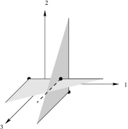
Figure 4. The intersection of the pairs $(x_{1}^{3}x_{3},\{2,3\})$ and $(x_{2}^{2}x_{3}^{2},\{1,3\})$ is the pair $(x_{1}^{3}x_{2}^{2}x_{3}^{2},\{3\})$.

Lemma 5.7.

Let $M\subset{\bf{k}}[{\bf{x}}]$ be a monomial ideal. Let $({\bf{x}}^{\bf{u}},\sigma)$ and $({\bf{x}}^{\bf{v}},\tau)$ be different standard pairs of $M$ with non-empty intersection $({\bf{x}}^{\textup{max}({\bf{u}},{\bf{v}})},\sigma\cap\tau)$. Then $\sigma\cap\tau$ is properly contained in each of $\sigma$ and $\tau$.

Proof:   Suppose $\sigma\cap\tau=\sigma$. Choose ${\bf{x}}^{\bf{m}}$ in the intersection of the two standard pairs. If $i\in\sigma$, $v_{i}=u_{i}=0$ since $\sigma\subseteq\tau$ and $({\bf{x}}^{\bf{u}},\sigma)$ and $({\bf{x}}^{\bf{v}},\tau)$ are admissible. If $i\in\overline{\sigma}$, we have $m_{i}=u_{i}$ since ${\bf{x}}^{\bf{m}}\in({\bf{x}}^{\bf{u}},\sigma)$ and $u_{i}=m_{i}\geq v_{i}$ since ${\bf{x}}^{\bf{m}}\in({\bf{x}}^{\bf{v}},\tau)$. In both cases $u_{i}\geq v_{i}$, implying ${\bf{u}}=\textup{max}({\bf{u}},{\bf{v}})$. Consequently $({\bf{x}}^{\bf{u}},\sigma)=({\bf{x}}^{\textup{max}({\bf{u}},{\bf{v}})},\sigma)=({\bf{x}}^{\textup{max}({\bf{u}},{\bf{v}})},\sigma\cap\tau)=({\bf{x}}^{\bf{u}},\sigma)\cap({\bf{x}}^{\bf{v}},\tau)\subseteq({\bf{x}}^{\bf{v}},\tau)$. This implies that $({\bf{x}}^{\bf{u}},\sigma)=({\bf{x}}^{\bf{v}},\tau)$ since both are standard pairs, which is a contradiction. $\square$

Lemma 5.8.

Let $M,M^{\prime}\subset{\bf{k}}[{\bf{x}}]$ be monomial ideals with $M\subseteq M^{\prime}$ and let $d$ be the Krull dimension of ${\bf{k}}[{\bf{x}}]/M$. Let ${\bf{a}}\in\mathbb{N}_{>0}^{n}$. Then the $d$-dimensional standard pairs of $M$ and $M^{\prime}$ are the same if and only if $H_{M,{\bf{a}}}-H_{M^{\prime},{\bf{a}}}\in{\mathcal{O}}(s^{d-2})$.

Proof:   $(\Rightarrow)$: We count the number of standard monomials of each monomial ideal via the Inclusion-Exclusion Principle, getting a formula of the form

$$|({\bf{x}}^{\alpha_{1}},\sigma_{1})_{s}\cup\dots\cup({\bf{x}}^{\alpha_{t}},\sigma_{t})_{s}|=\sum_{r=1}^{t}(-1)^{r-1}\sum_{1\leq i_{1}<\dots<i_{r}\leq t}|({\bf{x}}^{\alpha_{i_{1}}},\sigma_{i_{1}})_{s}\cap\dots\cap({\bf{x}}^{\alpha_{i_{r}}},\sigma_{i_{r}})_{s}|$$

for each of $M$ and $M^{\prime}$. The nonzero terms having $r\not=1$ or having $|\sigma_{i_{1}}|\not=d$ belong to ${\mathcal{O}}(s^{d-2})$ by Lemma 5.7 and Lemma 5.5. The remaining ones correspond to the $d$-dimensional standard pairs. Since the $d$-dimensional standard pairs of $M$ and $M^{\prime}$ are the same, these remaining terms are the same for both sums. Hence the difference $H_{M,{\bf{a}}}-H_{M^{\prime},{\bf{a}}}$ is in ${\mathcal{O}}(s^{d-2})$.

$(\Leftarrow)$: By Lemma 5.3, each term in the sum for $M^{\prime}$ that is not in ${\mathcal{O}}(s^{d-2})$ is also in the sum for $M$. Suppose there were more terms in the sum for $M$ not in ${\mathcal{O}}(s^{d-2})$. These terms would all be positive, so the difference $H_{M,{\bf{a}}}-H_{M^{\prime},{\bf{a}}}$ would not be in ${\mathcal{O}}(s^{d-2})$, a contradiction. $\square$

Lemma 5.9.

Let $I\subset{\bf{k}}[{\bf{x}}]$ be an ${\bf{a}}$-homogeneous ideal such that ${I_{{\mathcal{C}}_{\mathcal{A}}}}\subseteq I\subseteq{{I_{\mathcal{A}}}}$. Then $H_{I,{\bf{a}}}-H_{(I:x_{1}^{\infty}),{\bf{a}}}\in{\mathcal{O}}(s^{d-2})$.

Proof:   Let $\omega$ represent the ${\bf{a}}$-graded reverse lexicographic term order with $x_{1}\prec x_{2}\prec\dots\prec x_{n}$. Since $I\subseteq(I:x_{1}^{\infty})$ implies $\textup{in}_{\omega}(I)\subseteq\textup{in}_{\omega}(I:x_{1}^{\infty})$, it suffices (by Lemma 5.8) to show equality between the sets of $d$-dimensional standard pairs of these initial ideals to prove the lemma. Since ${I_{{\mathcal{C}}_{\mathcal{A}}}}\subseteq I\subseteq{{I_{\mathcal{A}}}}$, all ideals involved are $d$-dimensional.

Let $({\bf{x}}^{\bf{u}},\sigma)$ be a standard pair of $\textup{in}_{\omega}(I)$ with $|\sigma|=d$. Then by Remark 3.12, $(1,\sigma)$ is also a standard pair of $\textup{in}_{\omega}(I)$. Recall that the $\sigma$-columns of $A$ are independent over $\mathbb{Q}$ since $\sigma$ is a maximal face of $\Delta_{\omega}$. We claim that $1\in\sigma$. If not, then $a_{1}$ and $\{a_{i}\}_{i\in\sigma}$ are dependent over $\mathbb{Q}$. By Lemma 3.1 this gives an ${\bf{a}}$-homogeneous binomial ${\bf{x}}^{\alpha}-{\bf{x}}^{\beta}\in{I_{{\mathcal{C}}_{\mathcal{A}}}}\subseteq I$ with $\textup{supp}(\alpha),\textup{supp}(\beta)\subseteq\sigma\cup\{1\}$ and $\textup{supp}(\alpha)\cap\textup{supp}(\beta)=\emptyset$. The initial term $\textup{in}_{\omega}({\bf{x}}^{\alpha}-{\bf{x}}^{\beta})$ must be the term not containing $x_{1}$ by the definition of $\omega$, so the support of this term is contained in $\sigma$. This contradicts $(1,\sigma)$ being standard.

The ideal $\textup{in}_{\omega}(I:x_{1}^{\infty})$ can be computed from $\textup{in}_{\omega}(I)$ by projection along the $x_{1}$ axis, see [18, Lemma 12.1]. Since the monomials in $({\bf{x}}^{\bf{u}},\sigma)$ are all standard for $\textup{in}_{\omega}(I)$ with $1\in\sigma$, the pair $({\bf{x}}^{\bf{u}},\sigma)$ must be admissible for $\textup{in}_{\omega}(I:x_{1}^{\infty})$. It is standard because its root is 1 and its dimension is $d$. $\square$

Second proof of Theorem 3.19: Let ${\bf{a}}$ be a positive vector in the rowspan of $A$. By Proposition 4.1, we have ${{I_{\mathcal{A}}}}=({I_{{\mathcal{C}}_{\mathcal{A}}}}\,:\,(x_{1}x_{2}\cdots x_{n})^{\infty})=(({I_{{\mathcal{C}}_{\mathcal{A}}}}\,:\,x_{1}^{\infty})\,:\ldots\,:x_{n}^{\infty})$ so by repeatedly applying Lemma 5.9, we see that $H_{{{I_{\mathcal{A}}}},{\bf{a}}}-H_{{I_{{\mathcal{C}}_{\mathcal{A}}}},{\bf{a}}}\in{\mathcal{O}}(s^{d-2})$. It then follows by Lemma 5.8 that $\textup{in}_{\omega}({{I_{\mathcal{A}}}})$ and $\textup{in}_{\omega}({I_{{\mathcal{C}}_{\mathcal{A}}}})$ have the same $d$-dimensional standard pairs. $\square$

5.1. Polyhedral Fans of ${I_{{\mathcal{C}}_{\mathcal{A}}}}$

An ideal in ${\bf{k}}[{\bf{x}}]$ gives rise to several natural equivalence relations on $\mathbb{R}^{n}$ some of which give rise to polyhedral fans. In this final part, we compare various equivalence relations and fans for toric and circuit ideals.

Definition 5.10.

[16, page 112] Let $J\subset{\bf{k}}[{\bf{x}}]$ be an ideal and $d$ be the Krull dimension of ${\bf{k}}[{\bf{x}}]/J$. Define $\textup{top}(J)$ to be the intersection of all primary components of $J$ of dimension $d$.

Note that $\textup{top}(J)$ is well defined since the $d$-dimensional primary components of $J$ are not embedded and are hence unique.

Definition 5.11.

Let $I\subset{\bf{k}}[{\bf{x}}]$ be an ideal homogeneous with respect to a positive vector ${\bf{a}}\in\mathbb{N}_{>0}^{n}$. We define three equivalence relations on $\mathbb{R}^{n}$:

• The initial ideal equivalence relation ${\bf{u}}\sim{\bf{v}}\Leftrightarrow\textup{in}_{{\bf{u}}}(I)=\textup{in}_{{\bf{v}}}(I)$.

• The top equivalence relation ${\bf{u}}\sim{\bf{v}}\Leftrightarrow\textup{top}(\textup{in}_{{\bf{u}}}(I))=\textup{top}(\textup{in}_{{\bf{v}}}(I))$.

• The radical equivalence relation ${\bf{u}}\sim{\bf{v}}\Leftrightarrow\sqrt{\textup{in}_{{\bf{u}}}(I)}=\sqrt{\textup{in}_{{\bf{v}}}(I)}$.

In all three cases, the equivalence classes are invariant under translation by ${\bf{a}}$.

Definition 5.12.

A collection $C$ of polyhedra in $\mathbb{R}^{n}$ is a polyhedral complex if:

1. all proper faces of a polyhedron $P\in C$ are in $C$, and

2. the intersection of any two polyhedra $A,B\in C$ is a face of $A$ and $B$.

A polyhedral complex is a fan if it only consists of cones.

We say that an equivalence relation defines a fan $F$ if the closures of its equivalence classes are exactly the cones in $F$.

Proposition 5.13.

Let $I$ be as in Definition 5.11. Then

1. The initial ideal equivalence relation defines the Gröbner fan of $I$.

2. The radical equivalence relation does not define a fan in general.

A proof of the first claim is given in [18, Chapter 2]. See also [14]. The following example demonstrates the second claim.

Example 5.14.

The radical equivalence classes of the homogeneous ideal $I=\langle c^{4}-ba^{3},ab^{3}-ba^{3}\rangle\subset{\bf{k}}[a,b,c]$ are not all convex. This ideal has eight monomial initial ideals. Four of them have radical $\langle ab,ac,bc\rangle$ and the other four have radical $\langle ab,c\rangle$. The intersection of the Gröbner fan with the $2$-dimensional standard simplex is shown in Figure 5 and the two radical equivalence classes are shown in gray and white.

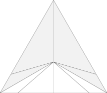
Figure 5. The Gröbner fan from Example 5.14 and the two radical equivalence classes. The fan is drawn in the standard simplex with $(1,0,0)$ at the right bottom, $(0,1,0)$ at the left bottom and $(0,0,1)$ at the top.

However, for toric ideals, all three equivalence relations of Definition 5.11 give rise to polyhedral fans.

Proposition 5.15.

1. The radical equivalence relation of ${{I_{\mathcal{A}}}}$ defines the secondary fan of $\mathcal{A}$.

2. The top equivalence relation of ${{I_{\mathcal{A}}}}$ defines the hypergeometric fan of $\mathcal{A}$.

Furthermore, the Gröbner fan of ${{I_{\mathcal{A}}}}$ is a refinement of the hypergeometric fan of $\mathcal{A}$, which is a refinement of the secondary fan of $\mathcal{A}$.

Proposition 5.15 may be taken as the definition of the hypergeometric and secondary fans of $\mathcal{A}$. The proposition is a collection of several known results [16, Proposition 3.3.1 and Corollary 3.3.2], [2], and [18, Chapter 8]. We now study the three equivalence classes for ${I_{{\mathcal{C}}_{\mathcal{A}}}}$.

Theorem 5.16.

The radical equivalence classes of ${I_{{\mathcal{C}}_{\mathcal{A}}}}$ form a polyhedral fan that coincides with the secondary fan of ${{I_{\mathcal{A}}}}$.

Proof:   By Proposition 5.15, to prove that the radical equivalence relation of ${I_{{\mathcal{C}}_{\mathcal{A}}}}$ defines the secondary fan of $\mathcal{A}$ it suffices to show that $\sqrt{\textup{in}_{\omega}({{I_{\mathcal{A}}}})}=\sqrt{\textup{in}_{\omega}({I_{{\mathcal{C}}_{\mathcal{A}}}})}$ for any $\omega$. Since ${I_{{\mathcal{C}}_{\mathcal{A}}}}\subseteq{{I_{\mathcal{A}}}}$ one inclusion is clear. To prove the other inclusion we first observe $\sqrt{\textup{in}_{\omega}({{I_{\mathcal{A}}}})}$ is $\omega$-homogeneous since $\textup{in}_{\omega}({{I_{\mathcal{A}}}})$ is. Hence it suffices to show that any homogeneous element in $\sqrt{\textup{in}_{\omega}({{I_{\mathcal{A}}}})}$ is also in $\sqrt{\textup{in}_{\omega}({I_{{\mathcal{C}}_{\mathcal{A}}}})}$. Let $f\in\sqrt{\textup{in}_{\omega}({{I_{\mathcal{A}}}})}$ be $\omega$-homogeneous. Then there exists some $m$ such that $f^{m}\in\textup{in}_{\omega}({{I_{\mathcal{A}}}})$. The polynomial $f^{m}$ is also $\omega$-homogeneous, so $f^{m}=\textup{in}_{\omega}(F)$ for some $F\in{{I_{\mathcal{A}}}}$. Since $\sqrt{{I_{{\mathcal{C}}_{\mathcal{A}}}}}={{I_{\mathcal{A}}}}$, $F^{k}\in{I_{{\mathcal{C}}_{\mathcal{A}}}}$ for some $k$, and $\textup{in}_{\omega}(F^{k})=\textup{in}_{\omega}(F)^{k}=f^{mk}$. Hence, $f\in\sqrt{\textup{in}_{\omega}({I_{{\mathcal{C}}_{\mathcal{A}}}})}$. $\square$

Now we consider the top equivalence relation of ${I_{{\mathcal{C}}_{\mathcal{A}}}}$.

Lemma 5.17.

[16, Lemma 3.2.4] Let $M\subseteq{\bf{k}}[{\bf{x}}]$ be a monomial ideal such that the Krull dimension of ${\bf{k}}[{\bf{x}}]/M$ is $d$. Then

$$\textup{top}(M)=\bigcap_{({\bf{x}}^{\bf{u}},\sigma)}\langle x_{i}^{{\bf{u}}_{i}+1}:i\not\in\sigma\rangle$$

where the intersection is taken over all $d$-dimensional standard pairs of $M$.

Lemma 5.18.

For any generic $\omega\in\mathbb{R}^{n}$, $\textup{top}(\textup{in}_{\omega}({{I_{\mathcal{A}}}}))=\textup{top}(\textup{in}_{\omega}({I_{{\mathcal{C}}_{\mathcal{A}}}}))$.

Proof:   For a generic $\omega$, the initial ideals $\textup{in}_{\omega}({{I_{\mathcal{A}}}})$ and $\textup{in}_{\omega}({I_{{\mathcal{C}}_{\mathcal{A}}}})$ are both $d$-dimensional monomial ideals, and by Lemma 5.17, their tops only depend on their $d$-dimensional standard pairs. By Theorem 3.19, these standard pairs are the same for both initial ideals. $\square$

Lemma 5.18 proves the following.

Proposition 5.19.

The top equivalence relation defines the same maximal cells for both ${{I_{\mathcal{A}}}}$ and ${I_{{\mathcal{C}}_{\mathcal{A}}}}$. These cells are precisely the open maximal cones in the hypergeometric fan of ${{I_{\mathcal{A}}}}$.

In contrast to Theorem 5.16 and Proposition 5.19, we have the following result for the initial ideal equivalence relation for ${{I_{\mathcal{A}}}}$ and ${I_{{\mathcal{C}}_{\mathcal{A}}}}$.

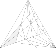
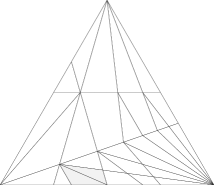
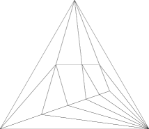
Figure 6. The Gröbner fans in the proof of Proposition 5.20 intersected with the simplex with coordinates $(0,1,0,0)$ (right), $(0,0,1,0)$ (left) and $(0,0,0,1)$ (top). The circuit fan is to the left and the toric fan is in the middle. The hypergeometric fan is shown to the right.

Proposition 5.20.

In general, neither is the Gröbner fan of ${{I_{\mathcal{A}}}}$ a refinement of the Gröbner fan of ${I_{{\mathcal{C}}_{\mathcal{A}}}}$, nor vice-versa.

Proof:   Let $A=(7\;9\;13\;15)$. It is easy to check that $\textup{in}_{(0,16,27,1)}({I_{{\mathcal{C}}_{\mathcal{A}}}})=\textup{in}_{(0,20,25,3)}({I_{{\mathcal{C}}_{\mathcal{A}}}})$ while $\textup{in}_{(0,16,27,1)}({{I_{\mathcal{A}}}})\not=\textup{in}_{(0,20,25,3)}({{I_{\mathcal{A}}}})$. Hence $(0,16,27,1)$ and $(0,20,25,3)$ lie in the same maximal cell of the Gröbner fan of ${I_{{\mathcal{C}}_{\mathcal{A}}}}$ but in different maximal cells of the Gröbner fan of ${{I_{\mathcal{A}}}}$. This proves that the Gröbner fan of ${I_{{\mathcal{C}}_{\mathcal{A}}}}$ does not refine the Gröbner fan of ${{I_{\mathcal{A}}}}$. On the other hand, $\textup{in}_{(0,4,19,9)}({{I_{\mathcal{A}}}})=\textup{in}_{(0,4,16,5)}({{I_{\mathcal{A}}}})$ and $\textup{in}_{(0,4,19,9)}({I_{{\mathcal{C}}_{\mathcal{A}}}})\not=\textup{in}_{(0,4,16,5)}({I_{{\mathcal{C}}_{\mathcal{A}}}})$. Hence the Gröbner fan of ${{I_{\mathcal{A}}}}$ does not refine the Gröbner fan of ${I_{{\mathcal{C}}_{\mathcal{A}}}}$. $\square$

The example in Proposition 5.20 would be best illustrated by a picture of the three-dimensional standard simplex in $\mathbb{R}^{n}$ intersected with the fans. Unfortunately we are limited to two dimensions in our drawing (Figure 6). The hypergeometric fan of ${{I_{\mathcal{A}}}}$ is drawn at the end of the two Gröbner fans.

Corollary 5.21.

If $n-d=2$ the Gröbner fan of ${I_{{\mathcal{C}}_{\mathcal{A}}}}$ is a refinement of the Gröbner fan of ${{I_{\mathcal{A}}}}$.

Proof:   Theorem 3.3.8 in [16] says that if $n-d=2$ then the Gröbner fan of ${{I_{\mathcal{A}}}}$ equals the hypergeometric fan of $\mathcal{A}$. The corollary then follows from Proposition 5.19 and the fact that the Gröbner fan of ${I_{{\mathcal{C}}_{\mathcal{A}}}}$ refines the hypergeometric fan of $\mathcal{A}$. $\square$

References

[1]
M.F. Atiyah and I.G. McDonald.
Introduction to Commutative Algebra.
Westview Press, Boulder, CO, 1969.
[2]
L. J. Billera, P. Filliman, and B. Sturmfels.
Constructions and complexity of secondary polytopes.
Advances in Mathematics, 83:155–179, 1990.
[3]
D. Cox, J. Little, and D. O’Shea.
Ideals, Varieties and Algorithms.
Springer-Verlag, New York, 1992.
[4]
P. Diaconis, D. Eisenbud, and B. Sturmfels.
Lattice walks and primary decomposition.
In B. E. Sagan and R. P. Stanley, editors, Mathematical Essays
in Honor of Gian-Carlo Rota, pages 173–193, Boston, 1998. Birkhäuser.
[5]
P. Diaconis and B. Sturmfels.
Algebraic algorithms for sampling from conditional distributions.
Annals of Statistics, 26:363–397, 1998.
[6]
D. Eisenbud and B. Sturmfels.
Binomial ideals.
Duke Math. J., pages 1–45, 1996.
[7]
G. Ewald.
Combinatorial Convexity and Algebraic Geometry, volume 168 of
Graduate Texts in Mathematics.
Springer-Verlag, New York, 1996.
[8]
W. Fulton.
Introduction to Toric Varieties.
Princeton University Press, 1993.
[9]
D. Grayson and M. Stillman.
Macaulay 2, a software system for research in algebraic geometry.
Available at http://www.math.uiuc.edu/Macaulay2.
[10]
S. Hoşten and B. Sturmfels.
GRIN : An implementation of Gröbner bases for integer
programming.
In E. Balas and J. Clausen, editors, Integer Programming and
Combinatorial Optimization, pages 267–276. Lecture Notes in Computer
Science 920, Springer Verlag, 1995.
[11]
S. Hoşten and R.R. Thomas.
The associated primes of initial ideals of lattice ideals.
Mathematical Research Letters, 6:83–97, 1999.
[12]
S. Hoşten and R.R. Thomas.
Gomory integer programs.
Math. Programming, Series B, 96:271–292, 2003.
[13]
A. Jensen.
Gfan, a software system for Gröbner fans.
Available at http://home.imf.au.dk/ajensen/software/gfan/gfan.html.
[14]
T. Mora and L. Robbiano.
The Gröbner fan of an ideal.
Journal of Symbolic Computation, 6:183–208, 1988.
[15]
H. Ohsugi.
Toric ideals and an infinite family of normal (0,1)-polytopes without
unimodular regular triangulations.
Discrete and Computational Geometry, 27:551–565, 2002.
[16]
M. Saito, B. Sturmfels, and N. Takayama.
Gröbner Deformations of Hypergeometric Differential
Equations, volume 6.
Algorithms and Computation in Mathematics, Springer-Verlag, New-York,
1999.
[17]
A. Schrijver.
Theory of Linear and Integer Programming.
Wiley-Interscience Series in Discrete Mathematics and Optimization,
New York, 1986.
[18]
B. Sturmfels.
Gröbner Bases and Convex Polytopes, volume 8 of University Lecture Series.
American Mathematical Society, Providence, RI, 1996.
[19]
B. Sturmfels, N. Trung, and W. Vogel.
Bounds on projective schemes.
Mathematische Annalen, 302:417–432, 1995.