Sergei V. Gusev

Department of Mathematics and Mechanics, St Petersburg State University
2 Bibliotechnaya sq., Peterhof, St.Petersburg, 198904, Russia
E-mail address: gusev@ieee.org

Igor A. Makarov

Institute for Problems of Mechanical Engineering, Russian Academy of Sciences
61 Bolshoy av., St.Petersburg, 199178, Russia
E-mail address: mak@ccs1.ipme.ru

Abstract

The paper considers a motion control problem for kinematic models of nonholonomic wheeled systems. The class of maneuverable wheeled systems is defined consisting of systems that can follow any sufficiently smooth non-stop trajectory on the plane. A sufficient condition for maneuverability is obtained. The design of control law that stabilizes motion along the desired trajectory on the plane is performed in two steps. On the first step the trajectory on the configuration manifold of the system and the input function are constructed that ensure the exact reproduction of the desired trajectory on the plane. The second step is the stabilization of the constructed trajectory on the configuration manifold of the system. For this purpose a recursive procedure is used that is a version of backstepping algorithm meant for non-stationary systems nonlinearly depending on input. The procedure results in the continuous memoryless feedback that stabilizes the trajectory on the configuration manifold of the system. As an example the motion control problem for a truck with multiple trailers is considered. It is shown that the proposed control law stabilizes the desired trajectory of the vehicle on the plane for all initial states of the system from some open dense submanifold of the configuration manifold, i. e., almost globally. The statement takes place both for a truck pulling any number of trailers in a forward direction and for a truck pushing any number of trailers in a backward direction. The latter result is the solution of the intuitively hard problem of the road train reverse motion control. The effectiveness of the proposed control is demonstrated by simulation. Animated examples are presented at Sergei V. Gusev Web Page.

Keywords: Nonholonomic systems, kinematics, nonlinear systems, trajectory tracking, backstepping.

AMS subject classification: 93D15; 70Q05; 70B15.

1.  Introduction.

The control of nonholonomic mechanical systems is a subject of intensive study (see survey [17]) that is mainly devoted to the transport robot control. These investigations can be classified into two groups: feedforward and feedback control strategies. The first direction, known as the motion planning problem, is presented in the comprehensive monograph [19]. The second direction can be subdivided into problems of the equilibrium manifold stabilization [2, 21], the zero state stabilization [2, 4, 6, 22, 26, 27, 29], and the stabilization of desired trajectory. Despite that latter problem is of great practical importance it is less investigated then other stabilization problems.

One approach to stabilization of the desired trajectory uses approximate linearization of the system in the neighborhood of this trajectory [1, 30]. Unfortunately, thus obtained linear feedback is guaranteed to perform well only in a small neighborhood of the desired trajectory.

Another approach is based on the system transformation to the chained form [27]. In [16] such a transformation is used for the trajectory stabilization of wheeled systems. Though the constructed feedback is not globally stabilizing its domain of attraction is not necessary a small neighborhood of the desired trajectory as in the previous case. However, this approach has a drawback that some trajectories, despite of being traceable in principle, are nevertheless missed in the domain of the transformation and hence they could not be stabilized. Thus the approach imposes unnecessary and unnatural restrictions on the desired trajectories of the system. For example, whether or not a particular trajectory is stabilizable might depend on the choice of a Cartesian coordinate system on the plane.

This paper deals with a specific variant of a trajectory tracking problem for wheeled systems. We select a point fixed in the body of the vehicle and are trying to define the vehicle control that stabilizes the motion of this distinguished point along a given trajectory on the plane. Note that when given a planar desired trajectory, we are not presented with the corresponding high-dimensional trajectory on the configuration manifold of the system. Therefore, we find the control in two steps: 1) the motion planning step during which we construct an input function and the corresponding trajectory on the configuration manifold of the system, so that the latter maps exactly onto the planar desired trajectory; 2) the stabilization step, wherein we stabilize the constructed trajectory.

The purpose of this paper is the design of the control law that stabilizes any non-stop motion of the distinguished point of the vehicle along any sufficiently smooth curve on the plane. To this end it is supposed that the system can trace any such a trajectory on the plane. Systems that have this property are called maneuverable.

We give a sufficient condition for maneuverability of wheeled systems. For systems that satisfy this condition the motion planning problem is solved, i.e., the algorithm is proposed that using the desired trajectory of the distinguished point constructs the corresponding trajectory on the configuration manifold of the system.

The stabilization of the constructed trajectory is based on a nonlinear state feedback transformation of the kinematic model of the system to a simplified cascaded form. The recursive application of a backstepping-like procedure to the cascaded system gives a continuous memoryless feedback that stabilizes the trajectory.

In our previous papers it was shown that a polar state transformation can be used to achieve the local stabilization of the desired trajectory in the case of caterpillar [10] and four-wheeled [20] mobile robots. Such a transformation allows to obtain the high performance practical control algorithm for trajectory tracking of the mobile platform [7].

This paper extends previous results using a more general state feedback transformation of the system. The constructed control law stabilizes the motion of a truck with multiple trailers along any non-stop trajectory that has a sufficient number of bounded derivatives. We tackle the task both for a truck pulling any number of trailers in a forward direction and even for a truck pushing any number of trailers in a backward direction. In addition, the stabilization is almost global in sense that the attraction domain of the trajectory is an open dense submanifold of the system configuration manifold.

For the Chaplygin sled, which is the simplest wheeled system, the constructed feedback is memoryless, continuous on the whole configuration manifold and guarantees the global stabilization of the desired trajectory. The latter example shows that the assumption about the non-stop character of the motion is essential. Because, a well known Brockett’s result [3] implies that a continuous memoryless feedback cannot globally stabilize the desired configuration of the Chaplygin sled.

The simulation shows the effectiveness of the proposed method of trajectory tracking control. The animated simulation is presented in [9]. Preliminary results on the maneuverable vehicles control can be found in [12].

Finally, we should note that while the present paper deals with kinematic models of wheeled systems, the obtained results can serve as the basis for the stabilization of dynamical models of vehicles (by analogy with results in [14], where the stabilization of the dynamical model of a car is considered) as well as for the adaptive control of robots using methods in [8, 11, 13, 14].

2.  Mathematical model of the system.

Wheeled vehicles are nonholonomic mechanical systems. We begin by describing the mathematical model of such systems. The configuration manifold of the system $\mathcal{Q}$ is the real smooth manifold with local coordinates $q=(q_{1},\ldots,q_{N}).$ Let $T_{q}\mathcal{Q}$ and $T^{\ast}_{q}\mathcal{Q}$ denote tangent and cotangent spaces of the manifold $\mathcal{Q}$ at a point $q,$ and let $T\mathcal{Q}=\bigcup_{q\in\mathcal{Q}}T_{q}\mathcal{Q}$ and $T^{\ast}\mathcal{Q}=\bigcup_{q\in\mathcal{Q}}T^{\ast}_{q}\mathcal{Q}$ denote tangent and cotangent bundles of this manifold. The kinematics of a nonholonomic system is described by a set of one-forms $\omega_{i}\in T^{\ast}\mathcal{Q},\;i=1,\ldots,n,$ that define the linear homogeneous nonholonomic constraints

$$\langle\omega_{j}(q),\dot{q}\rangle=0,\ \ \ j=1,\ldots,n,$$ (1)

where $\langle\omega(q),\dot{q}\rangle$ denote the action of the linear functional $\omega(q)\in T^{\ast}_{q}\mathcal{Q}$ on the tangent vector $\dot{q}\in T_{q}\mathcal{Q}.$ The trajectory of a nonholonomic system is the function $q\in C^{1}([0,\infty),\mathcal{Q})$ that satisfies the equations (1). Hereinafter $C^{k}(\mathcal{M}_{1},\mathcal{M}_{2}),\;k=0,1,2,\ldots,$ denotes the class of $k$ times continuously differentiable maps of the manifold $\mathcal{M}_{1}$ into the manifold $\mathcal{M}_{2}.$

Let $\mathcal{K}$ be an open submanifold of $\mathcal{Q}$ such that the codistribution $\Omega={\rm span}\left\{\omega_{1},\ldots,\omega_{n}\right\}\subset T^{\ast}\mathcal{Q}$ is constant-dimensional on $\mathcal{K}$. The codistribution $\Omega$ defines on $\mathcal{K}$ the $(m=N-n)$-dimensional distribution $\Delta=\Omega^{\bot}=\{g\in T\mathcal{K}\;|\;\langle\omega,g\rangle\equiv 0\;\forall\omega\in\Omega\}.$ We assume that smooth vectorfields $g_{1},\ldots,g_{m}$ form a basis of the distribution $\Delta.$ Then any lying in $\mathcal{K}$ trajectory of the nonholonomic system satisfies the differential equation

$$\dot{q}=\sum_{i=1}^{m}u_{i}g_{i}(q),$$ (2)

where $u=\mathop{\rm col}\nolimits(u_{1},\ldots,u_{m})\in C([0,\infty),R^{m}).$ Equation (2) is referred to as a kinematic model of the nonholonomic mechanical system. The freedom in defining the kinematic model is in the choice of the submanifold $\mathcal{K}$ and the basis vectorfields $g_{1},\ldots,g_{m}.$ We consider (2) as the equation that describes a control system with input $u.$

The wheeled system is a set of interconnected rigid bodies with wheels that can move on the plane. The wheels are constrained to roll without slipping. The position of the system on the plane is defined by the Cartesian coordinates $x_{1},x_{2}$ of a distinguished point, which is selected belonging to one of the wheel axles. Let $y_{1}$ be heading angle of the corresponding wheel, then the rolling without slipping constraint for this wheel takes the form

$$\dot{x}_{1}\sin y_{1}-\dot{x}_{2}\cos y_{1}=0.$$ (3)

We take a natural assumption that the constraint equations are invariant with respect to translations of the $x_{1},x_{2}$ plane.

It is typical for a vehicular system to have two scalar inputs. In terms of nonholonomic constraints it means that the number of constraints is two less then the number of degrees of freedom of the system.

Our assumptions can be summed up as follows:

1. $\mathcal{Q}=R^{2}\times\check{\mathcal{Q}},$ where $\check{\mathcal{Q}}$ is a smooth manifold of dimension $n.$ The vector of coordinates of the system can be represented as $q=\mathop{\rm col}\nolimits(x,y),$ where $x=\mathop{\rm col}\nolimits(x_{1},x_{2})$ is the vector of Cartesian coordinates of the distinguished point, and $y=\mathop{\rm col}\nolimits(y_{1},\ldots y_{n})$ are the remaining coordinates.

2. The kinematics of the system is described by the set of nonholonomic constraints (1) that includes the constraint (3).

3. The one-forms $\omega_{i},i=1,\ldots,n,$ do not depend on the coordinates $x_{1},x_{2}.$

Let $\mathcal{K}$ be an open submanifold of $\mathcal{Q}.$ It turns out that under very non-restrictive assumptions the wheeled system admits on $\mathcal{K}$ the kinematic model of the following special type

$$\begin{array}[]{lll}\dot{x}_{1}&=&u_{1}\cos y_{1},\\ \dot{x}_{2}&=&u_{1}\sin y_{1},\end{array}$$ (6)

$$\begin{array}[]{lll}\dot{y}&=&u_{1}h_{1}(y)+u_{2}h_{2}(y),\end{array}$$ (8)

where $u_{1}$ and $u_{2}$ are inputs, $u_{1}$ is the longitudinal velocity of the distinguished point motion along the vector $(\dot{x}_{1},\dot{x}_{2})\in R^{2},$ that has slope $y_{1},$ $h_{1},h_{2}\in T\check{\mathcal{Q}}.$ The output of the system is the distinguished point position $x=\mathop{\rm col}\nolimits(x_{1},x_{2}).$ Therefore the output trajectory of the system (6), (8) will be referred to as the distinguished point trajectory.

The control system (6), (8) is the subject of investigation in this paper.

Proposition 1

: Suppose the manifold $\mathcal{K}$ has the following properties:

• $\mathcal{K}=R^{2}\times\mathcal{Y},$ where $\mathcal{Y}$ is an open submanifold of $\check{\mathcal{Q}}.$

• The dimension of the codistribution $\Omega={\rm span}\left\{\omega_{1},\ldots,\omega_{n}\right\}$ is constant on $\mathcal{K}.$

• For any $q_{0}\in\mathcal{K}$ there exist the trajectory of the system $q\in C^{1}([-1,1]\rightarrow\mathcal{K}),$ passing through the point $q_{0}$ ($q(0)=q_{0}$), and such that $\dot{x}(0)\not=0.$

Then the wheeled system admits the kinematic model (6), (8) on the manifold $\mathcal{K}.$

The proof of Proposition 1 is given in Appendix A.

As an example consider the kinematic model of an automobile, the scheme of that is shown in Fig. 1. The vector of coordinates is $q=\mathop{\rm col}\nolimits(x_{1},x_{2},y_{1},y_{2}),$ where $x_{1}$ and $x_{2}$ are the Cartesian coordinates of the midpoint of the rear axle, $y_{1}$ is the heading angle, and $y_{2}$ is the angle between the front and rear axles. Define the configuration manifold as $\mathcal{Q}=R^{3}\times S^{1},$ where $S^{1}$ is the unit circle. From here on we shall employ the usual angular coordinate on the $S^{1}$ and we shall define trigonometric functions on $S^{1},$ where the argument will be the angle thus defined.

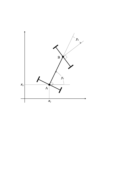
Figure 1: Kinematic scheme of an automobile (I).

Nonholonomic constraints take the form [23]

$$\begin{array}[]{l}\dot{x_{1}}\sin y_{1}-\dot{x_{2}}\cos y_{1}=0,\\ \dot{x_{1}}\sin(y_{1}+y_{2})-\dot{x_{2}}\cos(y_{1}+y_{2})-\dot{y_{1}}\cos y_{2}=0,\end{array}$$ (9)

where for simplicity the length of the automobile base (the segment AB) is assumed to be unity. The constraints (9) are defined by the one-forms $\omega_{1}(q)=\sin y_{1}dx_{1}-\cos y_{1}dx_{2},\;\omega_{2}(q)=\sin(y_{1}+y_{2})dx_{1}-\cos(y_{1}+y_{2})dx_{2}-\cos y_{2}dy_{1}.$ It is easy to see that $\mathcal{K}=\{q\in\mathcal{Q}\;|\;\cos y_{2}\not=0\}$ is the maximal submanifold of the manifold $\mathcal{Q},$ where the codistribution $\Omega={\rm span}\left\{\omega_{1},\omega_{2}\right\}$ is constant-dimensional. The defined on $\mathcal{K}$ kinematic model of an automobile has the known form [23]

$$\begin{array}[]{l}\dot{x}_{1}=u_{1}\cos y_{1},\\ \dot{x}_{2}=u_{1}\sin y_{1},\\ \dot{y}_{1}=u_{1}\tan y_{2},\\ \dot{y}_{2}=u_{2},\end{array}$$ (10)

where $u_{1}$ is the longitudinal velocity of the point A and $u_{2}$ is the angular velocity of the front axle spin relative to the automobile body.

Let us split the manifold $\mathcal{K}$ as $\mathcal{K}=R^{2}\times\mathcal{Y},$ where

$$\mathcal{Y}=\{y=(y_{1},y_{2})\in R\times S^{1}\;|\;\cos y_{2}\not=0\}.$$ (11)

Then the equation (10) takes the form (6), (8) with $h_{1}(y)=\mathop{\rm col}\nolimits(\tan y_{2},0),\;h_{2}(y)=\mathop{\rm col}\nolimits(0,1).$

3.  Maneuverable systems.

Let us consider the planar trajectory $x^{\mbox{\rm\tiny D}}\in C([0,\infty),R^{2})$ as the desired trajectory of the distinguished point of the system (6), (8).

Definition 1

: The trajectory $x^{\mbox{\rm\tiny D}}$ is called admissible trajectory of the distinguished point of the system (6), (8) if $x^{\mbox{\rm\tiny D}}\in C^{n+1}([0,\infty),R^{2})$ and

$$\inf_{t\geq 0}|\dot{x}^{\mbox{\rm\tiny D}}(t)|>0.$$ (12)

The set of all admissible trajectories of the distinguished point of the system (6), (8) is denoted $X\subset C^{n+1}([0,\infty),R^{2}).$

Definition 2

: The system (6), (8) is called maneuverable on an open submanifold $\mathcal{M}\subset\mathcal{K},$ if for any admissible trajectory of the distinguished point of the system there are the trajectory $q^{\mbox{\rm\tiny D}}=\mathop{\rm col}\nolimits(x^{\mbox{\rm\tiny D}},y^{\mbox{\rm\tiny D}})\in C^{1}([0,\infty),\mathcal{M})$ and the input $u^{\mbox{\rm\tiny D}}\in C([0,\infty),R^{2})$ that satisfy (6), (8). The operator $M:X\to C^{1}([0,\infty),\mathcal{M})\times C([0,\infty),R^{2}),$ which takes $x^{\mbox{\rm\tiny D}}$ to the pair $(q^{\mbox{\rm\tiny D}},u^{\mbox{\rm\tiny D}}),$ is called the maneuvering operator of the system. When $\mathcal{M}=\mathcal{K},$ the system is called maneuverable (without specifying the manifold).

A wheeled system is not necessary maneuverable. We shall demonstrate this with an example at the end of the section. The theorem below gives a sufficient condition for the wheeled system maneuverability. The proof of the theorem constructively defines the set of maneuvering operators for the system.

Let us introduce some notation. Consider a vector field $h$ and a function $\phi$ defined on a manifold $\mathcal{Y}.$ Denote $L_{h}\phi=\langle{\rm d}\phi,h\rangle=\sum_{i=1}^{k}\frac{\partial\phi}{\partial y_{i}}h^{(i)}$ the Lie derivative of the function $\phi$ along the vector field $h.$ The repeated Lie derivatives $L^{i}_{h}\phi,i=0,1,2,\ldots,$ are inductively defined by $L^{0}_{h}\phi=\phi$ and $L^{i}_{h}\phi=L_{h}L^{i-1}_{h}\phi,\;i\geq 1.$ In what follows we suppose that all manifolds, vectorfields, and functions are smooth enough to define all necessary Lie derivatives.

Theorem 1

: Let $\mathcal{O}\subset\mathcal{Y}$ be an open submanifold that is split as $\mathcal{O}=R\times\check{\mathcal{O}}.$ Suppose that for all $y\in\mathcal{O}$ the following conditions hold

$$L_{h_{2}}L_{h_{1}}^{i}y_{1}=0,\;i=0,\ldots,n-2,$$ (13)

$$L_{h_{2}}L_{h_{1}}^{n-1}y_{1}\not=0.$$ (14)

Then the smooth change of coordinates

$$s=S(y),$$ (15)

where the map $S\in C^{1}(\mathcal{O},R^{n})$ is defined by the equation

$$S(y)=\mathop{\rm col}\nolimits(L_{h_{1}}^{0}y,\ldots,L_{h_{1}}^{n-1}y),$$ (16)

and the nonsingular feedback transformation

$$v=F(y)u,$$ (17)

where the map $F\in C(\mathcal{O},GL(2))$ is defined by the equation

$$\begin{array}[]{lllllllllllllllllll}F(y)=\left[\begin{array}[]{ccccccccccccccccccccc}1,&0\\ L_{h_{1}}^{n}\phi(y),&L_{h_{2}}L_{h_{1}}^{n-1}\phi(y)\end{array}\right],\end{array}$$ (18)

transforms the system (6), (8) into the system

$$\begin{array}[]{l}\dot{x}_{1}=v_{1}\cos s_{1},\\ \dot{x}_{2}=v_{1}\sin s_{1},\end{array}$$ (21)

$$\begin{array}[]{l}\dot{s}_{i}=v_{1}s_{i+1},\;i=1,\ldots,n-1,\\ \dot{s}_{n}=v_{2}.\end{array}$$ (24)

If $S$ bijectively maps $\mathcal{O}$ on $R^{n},$ then the system (6), (8) is maneuverable on the manifold $\mathcal{M}=R^{2}\times\mathcal{O}.$

Remark 1

: Under the transformations (15) and (17) the equations $s_{1}=y_{1},v_{1}=u_{1}$ hold, and, consequently, the $x$-subsystem (6) does not change.

Proof. The representation (21), (24) can be obtained using the well known transformation of a nonlinear system to the canonical linear one [15]. However it is not difficult to prove this statement directly. Suppose that $y$ is the solution of the system (8) that corresponds to the input $u,$ and that $s$ and $v$ are defined by the transformations (15) and (17) respectively. Then from (13), (16), and (18) we obtain

$$\begin{array}[]{l}\dot{s}_{i}(t)=u_{1}(t)L^{i}_{h_{1}}y_{1}(t)+u_{2}(t)L_{h_{2}}L^{i-1}_{h_{1}}y_{1}(t)=v_{1}(t)s_{i+1}(t),\;i=1,\ldots,n-1,\end{array}$$

$$\begin{array}[]{l}\dot{s}_{n}(t)=u_{1}(t)L^{n}_{h_{1}}y_{1}(t)+u_{2}(t)L_{h_{2}}L^{n-1}_{h_{1}}y_{1}(t)=v_{2}(t).\end{array}$$

It is easy to see that, conversely, for any solution of (24) there corresponds some solution of (8), which is defined by the reverse transformation of variables.

Using (21), define the longitudinal velocity of the distinguished point that moves along the desired trajectory $x^{\mbox{\rm\tiny D}}$

$$v^{\mbox{\rm\tiny D}}_{1}(t)=\pm\sqrt{(\dot{x}^{\mbox{\rm\tiny D}}_{1}(t))^{2}+(\dot{x}^{\mbox{\rm\tiny D}}_{2}(t))^{2}},$$ (27)

where the sign of $v^{\mbox{\rm\tiny D}}_{1}$ can be chosen arbitrary but does not vary in time. Calculating $\dot{s}_{1}(t)$ by virtue of (21) with $v_{1}(t)=v^{\mbox{\rm\tiny D}}_{1}(t),$ we get

$$\dot{s}_{1}(t)=\displaystyle\frac{\ddot{x}^{\mbox{\rm\tiny D}}_{2}(t)\cos s_{1}-\ddot{x}^{\mbox{\rm\tiny D}}_{1}(t)\sin s_{1}}{v^{\mbox{\rm\tiny D}}_{1}(t)}.$$ (28)

Note that (12) implies the inequality $\inf_{t\geq 0}|v^{\mbox{\rm\tiny D}}_{1}(t)|>0.$ The desired heading angle $s^{\mbox{\rm\tiny D}}_{1}(t),\;t\geq 0,$ can be found as the solution of the differential equation (28) with the initial value $s^{\mbox{\rm\tiny D}}_{1}(0)$ that satisfies the equation

$$\dot{x}^{\mbox{\rm\tiny D}}(0)=v^{\mbox{\rm\tiny D}}_{1}(0)\left[\begin{array}[]{ccccccccccccccccccccc}\cos s^{\mbox{\rm\tiny D}}_{1}(0)\\ \sin s^{\mbox{\rm\tiny D}}_{1}(0)\end{array}\right].$$ (29)

Define $s^{\mbox{\rm\tiny D}}(t)$ using the recursive formulae

$$s^{\mbox{\rm\tiny D}}_{i}(t)=\dot{s}^{\mbox{\rm\tiny D}}_{i-1}(t)/v^{\mbox{\rm\tiny D}}_{1}(t),\ i=2,\ldots,n,$$ (30)

and put

$$v^{\mbox{\rm\tiny D}}_{2}(t)=\dot{s}^{\mbox{\rm\tiny D}}_{n}(t).$$ (31)

Then the triplet $x^{\mbox{\rm\tiny D}},s^{\mbox{\rm\tiny D}},v^{\mbox{\rm\tiny D}}$ satisfies the system of differential equations (21), (24). Since the transformation $S$ is diffeomorphism $\mathcal{O}$ onto $R^{n},$ we can define the trajectory

$$y^{\mbox{\rm\tiny D}}(t)=S^{-1}(s^{\mbox{\rm\tiny D}}(t)),$$ (32)

which satisfies the inclusion $y^{\mbox{\rm\tiny D}}(t)\in\mathcal{O}$ for all $t\geq 0.$ The desired input $u^{\mbox{\rm\tiny D}}$ can be uniquely defined from the equation

$$u^{\mbox{\rm\tiny D}}(t)=F^{-1}(y^{\mbox{\rm\tiny D}}(t))v^{\mbox{\rm\tiny D}}(t),$$ (33)

because the matrix $F(y)$ is nonsingular in $\mathcal{O}.$ The triplet $x^{\mbox{\rm\tiny D}},y^{\mbox{\rm\tiny D}},u^{\mbox{\rm\tiny D}}$ satisfies (6), (8).  

The proof gives the procedure for determining the maneuvering operators for the system (6), (8). After choosing the sign of $v^{\mbox{\rm\tiny D}}_{1}$ in (27) and the initial value $s^{\mbox{\rm\tiny D}}_{1}(0)$ satisfying (29), the formulae (27) – (33) uniquely define the pair $q^{\mbox{\rm\tiny D}}=\mathop{\rm col}\nolimits(x^{\mbox{\rm\tiny D}},y^{\mbox{\rm\tiny D}}),u^{\mbox{\rm\tiny D}}$ for a given admissible trajectory $x^{\mbox{\rm\tiny D}}.$

As an example of Theorem 1 application let us show that the kinematic model of an automobile (10) is maneuverable. The manifold $\mathcal{Y}$ defined by (11) is disconnected and consists of two connected components. It is easy to see that the conditions (13) and (14) of Theorem 1 are fulfilled on each component. For definiteness choose one component $\mathcal{O}=\{(y_{1},y_{2})\in R^{2}\;|\;|y_{2}|<\pi/2\}.$ On $\mathcal{O}$ the formulae (16) and (18) define the state transformation $S(y)=\mathop{\rm col}\nolimits(y_{1},\tan y_{2})$ and the feedback transformation $v_{1}=u_{1},\;v_{2}=u_{2}\cos^{-2}y_{2}.$ The system (10) is maneuverable on the manifold $\mathcal{O}\times R^{2}$ because $S$ bijectively maps $\mathcal{O}$ onto $R^{2}.$

In this example the choice of sign ”+” in (27) defines the trajectory $q^{\mbox{\rm\tiny D}}$ and the input $u^{\mbox{\rm\tiny D}}$ that correspond to an automobile forward motion along the desired trajectory $x^{\mbox{\rm\tiny D}},$ whereas the sign ”-” in (27) corresponds to an automobile backward motion along the same trajectory $x^{\mbox{\rm\tiny D}}.$

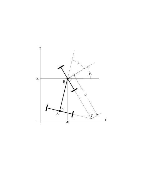
Figure 2: Kinematic scheme of an automobile (II).

Our next example shows that not any wheeled system is maneuverable and, more over, the maneuverability of the system depends on the choice of coordinates. Let us define the coordinates of automobile as follows: $x_{1},x_{2}$ are the Cartesian coordinates of the distinguished point B, which is the midpoint of the front axle, $y_{1}$ is the heading angle of the front wheels, $y_{2}$ is the angle between the front and rear axles (see Fig. 2). The configuration manifold of the system is $\mathcal{Q}=R^{3}\times S^{1}$ and can be split as $\mathcal{Q}=R^{2}\times\mathcal{Y},$ where $\mathcal{Y}=R\times S^{1}.$ The kinematic model is defined on the whole manifold $\mathcal{Q}$ and takes the form (6), (8) with $h_{1}(y)=\mathop{\rm col}\nolimits(\sin y_{2},0),\;h_{2}(y)=\mathop{\rm col}\nolimits(1,1).$ It is easy to see that conditions of Theorem 1 are not fulfilled for this system.

In fact, this system is not maneuverable. To show this let us construct the trajectory $x^{\mbox{\rm\tiny D}}$ that cannot be traced by the system. From Fig. 2 it is clear that at each instant of time $t$ the curvature of the point B trajectory is equal to $1/\rho(t),$ where $\rho(t)$ is the length of the hypotenuse of triangle ABC. Hence, $\rho(t)\geq 1$ for all $t\geq 0.$ It follows that the system cannot trace any trajectory $x^{\mbox{\rm\tiny D}}$ the curvature of which is less than one at some instant of time $t\geq 0.$ Thus the considered system is not maneuverable.

4.  Formulation of the trajectory stabilization problem.

Let $x^{\mbox{\rm\tiny D}}$ be a desired trajectory of the distinguished point of the system. The problem under consideration is to stabilize the motion of the distinguished point with coordinates $x$ along the desired trajectory $x^{\mbox{\rm\tiny D}}.$ But it is important also to guarantee boundedness of the control input of the system. Otherwise the stabilization has no practical application. For the input to be bounded, it does not suffice to assume the admissibility of the trajectory; more strict requirements have to be satisfied.

Definition 3

: The trajectory $x^{\mbox{\rm\tiny D}}$ of the distinguished point of the system (6), (8) is called strongly admissible if it is admissible and, in addition, all its derivatives up to the order $n+1$ are bounded, i. e., $\sup_{t\geq 0}\max_{k=1,\ldots,n+1}|d^{k}/dt^{k}x^{\mbox{\rm\tiny D}}(t)|<+\infty.$

The set of strongly admissible trajectories of the distinguished point of the system (6), (8) is denoted $\bar{X}.$

For maneuverable systems the problem under consideration can be refined. Let the system (6), (8) be maneuverable on the manifold $\mathcal{M}=R^{2}\times\mathcal{O}.$ Then for any admissible trajectory on the plane $x^{\mbox{\rm\tiny D}}$ the maneuvering operator $M$ defines the trajectory $q^{\mbox{\rm\tiny D}}=\mathop{\rm col}\nolimits(x^{\mbox{\rm\tiny D}},y^{\mbox{\rm\tiny D}})$ of the system (6), (8) and the input $u^{\mbox{\rm\tiny D}}$ such that the trajectory lies in $\mathcal{M}$ and corresponds to the input $u^{\mbox{\rm\tiny D}}.$ In this case becomes possible to replace stabilization of the desired planar trajectory $x^{\mbox{\rm\tiny D}}$ with that of the trajectory $q^{\mbox{\rm\tiny D}}.$ Clearly, the solution of the latter, more general problem, implies the solution for the problem of tracking the trajectory $x^{\mbox{\rm\tiny D}}.$

Suppose that $d$ is a metric on the manifold $\mathcal{O}.$ Consider a map $\Phi\in C(\mathcal{M}\times\mathcal{M}\times\mathcal{U},R^{2}),$ where $\mathcal{U}=\{u\in R^{2}\;|\;u_{1}\not=0\}.$

Definition 4

: The feedback

$$u=\Phi(q,q^{\mbox{\rm\tiny D}}(t),u^{\mbox{\rm\tiny D}}(t)),$$ (34)

where $q=\mathop{\rm col}\nolimits(x,y),\;q^{\mbox{\rm\tiny D}}=\mathop{\rm col}\nolimits(x^{\mbox{\rm\tiny D}},y^{\mbox{\rm\tiny D}}),$ stabilizes the trajectory $q^{\mbox{\rm\tiny D}}$ in $\mathcal{M},$ if for any initial value $q(0)\in\mathcal{M}$ the solution of the closed-loop system (6), (8), (34) is defined and lies in $\mathcal{M}$ for all $t\geq 0,$ and if the following limits hold:

$$\displaystyle\lim_{t\to\infty}(x(t)-x^{\mbox{\rm\tiny D}}(t))=0,$$ (35)

$$\displaystyle\lim_{t\to\infty}d(y(t),y^{\mbox{\rm\tiny D}}(t))=0,$$ (36)

$$\displaystyle\lim_{t\to\infty}(u(t)-u^{\mbox{\rm\tiny D}}(t))=0.$$ (37)

This definition implies, in particular, that if the input function $u^{\mbox{\rm\tiny D}}$ is bounded, so will be the input $u$ of the closed-loop system.

Now we return to the problem of the desired trajectory $x^{\mbox{\rm\tiny D}}$ stabilization. Consider an operator $U:[0,+\infty)\times\mathcal{M}\times\bar{X}\to\mathcal{U},$ which for $t\in[0,+\infty),\;q\in\mathcal{M},$ and $x^{\mbox{\rm\tiny D}}\in\bar{X}$ is defined as the superposition

$$U(t,q,x^{\mbox{\rm\tiny D}})=\Phi(q,q^{\mbox{\rm\tiny D}}(t),u^{\mbox{\rm\tiny D}}(t)),$$ (38)

where

$$(q^{\mbox{\rm\tiny D}},u^{\mbox{\rm\tiny D}})=M(x^{\mbox{\rm\tiny D}}).$$ (39)

Definition 5

: We say that the control law

$$u=U(t,q,x^{\mbox{\rm\tiny D}})$$ (40)

where the operator $U$ is defined by (38), (39), solves the problem of stabilizing the distinguished point trajectories of the system (6), (8) on the manifold $\mathcal{M}$, if for any strongly admissible trajectory $x^{\mbox{\rm\tiny D}}$ the feedback (34) stabilizes the trajectory $q^{\mbox{\rm\tiny D}}$ defined by (39).

The prime objective of the paper is solving the trajectories stabilization problem for the wheeled system (6), (8) on the manifold where the system is maneuverable. To do this it is necessary to design two operators $M$ and $\Phi.$ The former is already defined by Theorem 1. The latter is constructed in Section 5.

An additional objective is to make as wide as possible the domain where the constructed control law solves the trajectories stabilization problem. From the practical standpoint it is desirable to design the control law that solves this problem on the whole configuration manifold of the system $\mathcal{Q},$ i.e., globally. Such a control law for the Chaplygin sled is described below, in Section 6. The general problem of global stabilization of trajectories is not solved in the paper. However, we believe our result closely approximates the goal of the global stabilization. Let us explain in what sense.

Suppose that $\mathcal{K}=\bigcup_{i=1}^{m}\mathcal{M}_{i},$ where $\mathcal{M}_{i},\;i=1,\dots,m,$ are disjoint open connected components of $\mathcal{K},$ and for every $i=1,\dots,m,$ an operator $U_{i}:[0,+\infty)\times\mathcal{M}_{i}\times\bar{X}\to\mathcal{U}$ is defined. Consider an operator $U:[0,+\infty)\times\mathcal{K}\times\bar{X}\to\mathcal{U}$ defined for $t\in[0,+\infty),q\in\mathcal{K},x^{\mbox{\rm\tiny D}}\in\bar{X}$ by the equation

$$U(t,q,x^{\mbox{\rm\tiny D}})=U_{i}(t,q,x^{\mbox{\rm\tiny D}}),\mbox{\rm~{}if~{} }q\in\mathcal{M}_{i}.$$ (41)

Definition 6

: We say that the control law (40) with the operator (41) solves the problem of almost global stabilization of the distinguished point trajectories of the system (6), (8), if the manifold $\mathcal{K}$ is dense in the configuration manifold $\mathcal{Q},$ and if for every $i=1,\dots,m,$ the control law (40) with $U=U_{i},$ solves the problem of stabilizing the distinguished point trajectories of the system (6), (8) on the manifold $\mathcal{M}_{i}.$

In the sense of this definition we shall show that the proposed below control law solves the problem of almost global stabilization of the distinguished point trajectories for the considered in Section 6 kinematic model of a truck with multiple trailers.

5.  Stabilization of trajectories.

Suppose that the system (6), (8) satisfies the conditions of Theorem 1 on the manifold $\mathcal{M}$ and that $M$ is a corresponding maneuvering operator. Let $x^{\mbox{\rm\tiny D}}$ be an admissible trajectory of the distinguished point. Using the operator $M,$ define the trajectory $q^{\mbox{\rm\tiny D}}=\mathop{\rm col}\nolimits(x^{\mbox{\rm\tiny D}},y^{\mbox{\rm\tiny D}})$ and the input $u^{\mbox{\rm\tiny D}}$ ($(q^{\mbox{\rm\tiny D}},u^{\mbox{\rm\tiny D}})=M(x^{\mbox{\rm\tiny D}})$). After the state feedback transformation (15), (17) the system (6), (8) takes on the cascaded form (21), (24) and our design of the stabilizing feedback is based on that form. Using the state transformation (15) define the trajectory $s^{\mbox{\rm\tiny D}}(t)=S(y^{\mbox{\rm\tiny D}}(t)),$ $s^{\mbox{\rm\tiny D}}\in C^{1}([0,+\infty),R^{n}).$ To apply the backstepping technics we shall represent the system (21), (24) in terms of deviations from the trajectory $(x^{\mbox{\rm\tiny D}},s^{\mbox{\rm\tiny D}}).$

5.1. Further transformation of the kinematic model. Consider the function $\tau(t)=\int_{0}^{t}\sqrt{(\dot{x}^{\mbox{\rm\tiny D}}_{1}(\kappa))^{2}+(\dot{x}^{\mbox{\rm\tiny D}}_{2}(\kappa))^{2}}d\kappa;$ the value $\tau(t)$ is the length of the path traveled by the distinguished point in a time $t.$ Due to the equality $\dot{\tau}(t)=|\dot{x}^{\mbox{\rm\tiny D}}(t)|$ and the inequality (12), the function $\tau(.)$ maps the interval $[0,\infty)$ bijectively onto itself. The inverse function is denoted $t(.).$

Define functions $\bar{x}(\tau)=x^{\mbox{\rm\tiny D}}(t(\tau)),\bar{s}(\tau)=s^{\mbox{\rm\tiny D}}(t(\tau)),\bar{v}(\tau)=v^{\mbox{\rm\tiny D}}(t(\tau)),\tilde{x}(\tau)=x(t(\tau))-x^{\mbox{\rm\tiny D}}(t(\tau)),$ and $\tilde{s}(\tau)=s(t(\tau))-s^{\mbox{\rm\tiny D}}(t(\tau)).$ The change of variables from $t,x,s$ to $\tau,\tilde{x},\tilde{s}$ transforms the system (21), (24) into

$$\begin{array}[]{rcl}\tilde{x}^{\prime}&=&-\bar{w}_{1}\left[\begin{array}[]{ccccccccccccccccccccc}\cos\bar{s}_{1}\\ \sin\bar{s}_{1}\end{array}\right]+w_{1}G(\bar{s}_{1})\left[\begin{array}[]{ccccccccccccccccccccc}\cos\tilde{s}_{1}\\ \sin\tilde{s}_{1}\end{array}\right],\end{array}$$ (47)

$$\begin{array}[]{rcl}\tilde{s}^{\prime}_{i}&=&w_{1}\tilde{s}_{i+1}+(w_{1}-\bar{w}_{1})\bar{s}_{i+1},\indent i=1,\ldots,n-1,\\ \tilde{s}^{\prime}_{n}&=&w_{2},\end{array}$$ (50)

where

$$G(\bar{s}_{1})=\left[\begin{array}[]{ccccccccccccccccccccc}\cos\bar{s}_{1}&-\sin\bar{s}_{1}\\ \sin\bar{s}_{1}&\cos\bar{s}_{1}\end{array}\right],$$

$$w_{1}(\tau)=v_{1}(t(\tau))/|\bar{v}_{1}(\tau)|,\;w_{2}(\tau)=(v_{2}(t(\tau))-\bar{v}_{2}(\tau))/|\bar{v}_{1}(\tau)|.$$ (51)

Note that $\bar{w}_{1}=\bar{v}_{1}/|\bar{v}_{1}|=\mbox{\rm sign }\bar{v}_{1}$ does not depend on $\tau.$ Hereafter the prime denotes the differentiation with respect to $\tau.$ The above transformation uses the following formulae: $\bar{v}_{1}(\tau)=u^{\mbox{\rm\tiny D}}_{1}(t(\tau)),$

$$G(\bar{s}_{1})\left[\begin{array}[]{ccccccccccccccccccccc}\cos\tilde{s}_{1}\\ \sin\tilde{s}_{1}\end{array}\right]=\left[\begin{array}[]{ccccccccccccccccccccc}\cos(\tilde{s}_{1}+\bar{s}_{1})\\ \sin(\tilde{s}_{1}+\bar{s}_{1})\end{array}\right],$$

$$\begin{array}[]{lcl}{\bar{x}}^{\prime}_{1}&=&\bar{w}_{1}\cos\bar{s}_{1},\\ {x}^{\prime}_{2}&=&\bar{w}_{1}\sin\bar{s}_{1},\end{array}$$ (54)

$$\begin{array}[]{lcl}{\bar{s}}^{\prime}_{i}&=&\bar{w}_{1}\bar{s}_{i+1},\indent i=1,\ldots,n-1,\\ {\bar{s}}^{\prime}_{n}&=&\bar{v}_{2}/|\bar{v}_{1}|.\end{array}$$ (57)

5.2. Cascaded system stabilization theorem. To design a stabilizing feedback for the system (47), (50) we use a recursive procedure based on the idea of backstepping [18]. Let us formulate one step of the procedure.

Consider the cascaded system

$$z^{\prime}=B(z,\zeta,p(\tau)),$$ (58)

$$\zeta^{\prime}=b(z,\zeta,p(\tau))+\beta(z,\zeta,p(\tau))\upsilon,$$ (59)

where $z\in R^{k_{z}},\zeta,\upsilon\in R,\tau\geq 0,$ $p\in C^{1}([0,\infty),R^{k_{p}}),$ $B,\displaystyle\frac{\partial B}{\partial\zeta}\in C(R^{k_{z}}\times R\times R^{k_{p}},R^{k_{z}}),$ $b,\beta\in C(R^{k_{z}}\times R\times R^{k_{p}},R),$ $\beta(z,\zeta,p(\tau))\neq 0$ for all $z,\zeta,\tau.$

Suppose functions $\alpha\in C^{1}(R^{k_{z}}\times R^{k_{r}},R)$ and $V\in C^{1}(R^{k_{z}}\times R^{k_{p}}\times R^{k_{r}},R)$ are given that satisfy the conditions

$$\forall r\;\;\alpha(0,r)=0,$$ (60)

$$\forall\;p,r\;\;V(0,p,r)=0,$$ (61)

$$\forall\;z\not=0,p,r\;\;V(z,p,r)>0,$$ (62)

$$\forall\varepsilon>0,\mathcal{E}>0\;\inf_{|z|>\varepsilon,\;\max(|p|,|r|)<\mathcal{E}}V(z,p,r)>0.$$ (63)

Define a function $\hat{\alpha}:R^{k_{z}+1}\times R^{k_{p}}\times R^{k_{r}}\times R^{k_{r}}\to R$ by

$$\begin{array}[]{ll}\hat{\alpha}(\hat{z},p,r,r_{1})=&{\beta(z,\zeta,p)^{-1}}\left[\displaystyle\frac{\partial\alpha(z,r)}{\partial z}B(z,\zeta,p)+\displaystyle\frac{\partial\alpha(z,r)}{\partial r}r_{1}-\right.\\ &\left.\delta^{-1}\displaystyle\frac{\partial V(z,p,r)}{\partial z}D(z,\zeta,\alpha(z,r),p)-b(z,\zeta,p)-\gamma(\zeta-\alpha(z,r))\right],\end{array}$$ (64)

where

$$D(z,\zeta,\eta,p)=\left\{\begin{array}[]{ll}\displaystyle\frac{B(z,\zeta,p)-B(z,\eta,p)}{\zeta-\eta},&\mbox{\rm if }\zeta\not=\eta,\\ \displaystyle\frac{\partial B(z,\zeta,p)}{\partial\zeta},&\mbox{\rm if }\zeta=\eta,\end{array}\right.$$

and a function $\hat{V}:R^{k_{z}+1}\times R^{k_{p}}\times R^{k_{r}}\to R$ by

$$\hat{V}(\hat{z},p,r)=V(z,p,r)+\delta(\zeta-\alpha(z,r))^{2}/2.$$ (65)

Here $\gamma>0,\;\delta>0$ are parameters, $z\in R^{k_{z}},\;\zeta,\eta\in R,\;\hat{z}=\mathop{\rm col}\nolimits(z,\zeta),\;\;p\in R^{k_{p}},\;r,r_{1}\in R^{k_{r}}.$

Theorem 2

: The function $\hat{\alpha}$ is continuous, the function $\hat{V}$ is differentiable and satisfies the conditions (61)–(63), where $z$ should be replaced with $\hat{z}.$

• If the derivative of the function $V(z(\tau),p(\tau),r(\tau))$ along the trajectories of the closed-loop system (58),

  $$\zeta=\alpha(z,r(\tau))$$ (66)

  satisfies the inequality

  $$V^{\prime}(z(\tau),p(\tau),r(\tau))\leq-2\gamma V(z(\tau),p(\tau),r(\tau)),$$ (67)

  then the derivative of the function $\hat{V}(z(\tau),p(\tau),r(\tau))$ along the trajectories of the closed-loop system (58), (59),

  $$\upsilon=\hat{\alpha}(\hat{z},p(\tau),r(\tau),r^{\prime}(\tau))$$ (68)

  satisfies the inequality

  $$\hat{V}^{\prime}(\hat{z}(\tau),p(\tau),r(\tau))\leq-2\gamma\hat{V}(\hat{z}(\tau),p(\tau),r(\tau)).$$ (69)

• If the functions $p,r$ are bounded and the inequality (69) holds on the solutions of the system (58), (59), (68), then this system is globally asymptotically stable.

• If

  $$\forall p\in R^{k_{p}}\;\;B(0,0,p)=0\;\mbox{\rm~{}and~{}}b(0,0,p)=0,$$ (70)

  then

  $$\forall p\in R^{k_{p}},\;r,r_{1}\in R^{k_{r}}\;\;\hat{\alpha}(0,p,r,r_{1})=0.$$ (71)

• If, in addition to listed assumptions, the function $r^{\prime}$ is bounded, then

  $$\lim_{\tau\to\infty}\hat{\alpha}(\hat{z}(\tau),p(\tau),r(\tau),r^{\prime}(\tau))=0$$ (72)

  holds on the solutions of the closed-loop system (58), (59), (68).

Proof. The continuity of the function $\hat{\alpha}$ follows from (64) and properties of functions $\alpha,B,b,\beta,$ and $V.$ It should be noted that the function $1/\beta$ is defined and continuous for all $z\in R^{k_{z}},\;\zeta\in R,\;\tau\geq 0$ because $\beta$ is continuous and non-vanishing and that the function $D(z,\zeta,\alpha(z,r),r)$ is defined and continuous for all $z\in R^{k_{z}},\;\zeta\in R,\;r\in R^{k_{r}}$ due to the continuity of the functions $B$ and $\displaystyle\frac{\partial B}{\partial\zeta}.$

Let us show that $\hat{V}$ satisfies the conditions (61) – (63). The equality (61) is obvious.

Consider the inequality (62). Let $\hat{z}=\mathop{\rm col}\nolimits(z,\zeta)\not=0.$ We have $\hat{V}(\hat{z},p,r)>0$ for $z\not=0,$ since $\hat{V}(\hat{z},p,r)\geq V(z,p,r).$ If $z=0$ then $\hat{V}(\hat{z},p,r)=\delta(\zeta-\alpha(0,r))^{2}/2,$ and, by virtue of (60), $\hat{V}(\hat{z},p,r)=\zeta^{2}/2>0$ for $\zeta\not=0.$ The inequality (62) is proved.

We show (63) by reductio ad absurdum. Suppose this inequality is not fulfilled. Then there are $\varepsilon>0,$ $\mathcal{E}>0,$ and sequences $\{\hat{z}_{\kappa}\}_{\kappa=1}^{\infty},$ $\{r_{\kappa}\}_{\kappa=1}^{\infty},$ $\{p_{\kappa}\}_{\kappa=1}^{\infty},$ $(|\hat{z}_{\kappa}|>\varepsilon,\;|{r}_{\kappa}|<\mathcal{E},\;|{p}_{\kappa}|<\mathcal{E},\;\kappa=1,2,\ldots)$ such that

$$\lim_{\kappa\to\infty}\hat{V}(\hat{z}_{\kappa},p_{\kappa},r_{\kappa})=0.$$ (73)

Let $\hat{z}_{\kappa}=\mathop{\rm col}\nolimits(z_{\kappa},\zeta_{\kappa}).$ Then by virtue of (73),

$$\lim_{\kappa\to\infty}{V}({z}_{\kappa},p_{\kappa},r_{\kappa})=0.$$ (74)

The limit (74) and the inequality (63) imply

$$\lim_{\kappa\to\infty}z_{\kappa}=0.$$ (75)

From the continuity of the function $\alpha$ and the limit (75) it follows that

$$\lim_{\kappa\to\infty}\alpha(z_{\kappa},r_{\kappa})=0.$$ (76)

The substitution of (75) and (76) in (73) gives $\displaystyle\lim_{\kappa\to\infty}\zeta_{\kappa}=0$ and, consequently, $\displaystyle\lim_{\kappa\to\infty}\hat{z}_{\kappa}=0.$ The latter contradicts the assumption made about the sequence $\{\hat{z}_{\kappa}\}_{\kappa=1}^{\infty}.$ This contradiction proves that the function $\hat{V}$ satisfies (63).

The derivative of the function $\hat{V}$ along the trajectories of the closed-loop system (58), (59), (68) has the form

$$\hat{V}^{\prime}(\hat{z},p,r)=\displaystyle\frac{\partial V(z,p,r)}{\partial z}B(z,\zeta,p)+\displaystyle\frac{\partial V(z,p,r)}{\partial p}p^{\prime}+\displaystyle\frac{\partial V(z,p,r)}{\partial r}r^{\prime}+$$

$$\delta(\zeta-\alpha(z,r))[b(z,\zeta,p)+\beta(z,\zeta,p)\upsilon-\displaystyle\frac{\partial\alpha(z,r)}{\partial z}B(z,\zeta,p)-\displaystyle\frac{\partial\alpha(z,r)}{\partial r}r^{\prime}]$$

$$=\left\{\displaystyle\frac{\partial V(z,p,r)}{\partial z}B(z,\alpha(z,r),p)+\displaystyle\frac{\partial V(z,p,r)}{\partial p}p^{\prime}+\displaystyle\frac{\partial V(z,p,r)}{\partial r}r^{\prime}\right\}+$$

$$\left\{\displaystyle\frac{\partial V(z,p,r)}{\partial z}B(z,\zeta,p)-\displaystyle\frac{\partial V(z,p,r)}{\partial z}B(z,\alpha(z,r),p)+\right.$$

$$\left.\delta(\zeta-\alpha(z,r))[b(z,\zeta,p)+\beta(z,\zeta,p)\upsilon-\displaystyle\frac{\partial\alpha(z,r)}{\partial z}B(z,\zeta,p)-\displaystyle\frac{\partial\alpha(z,r)}{\partial r}r^{\prime}]\right\}.$$

The expression in the first curly braces is the derivative of $V$ along the trajectories of the system (58), (66). By virtue of (64), the term in the second curly braces is equal to $-\gamma\delta(\zeta-\alpha(z,r))^{2}.$ Thus, taking into account (67), we obtain (69).

The inequality (69) implies that the limit

$$\lim_{\tau\to\infty}\hat{V}(\hat{z}(\tau),p(\tau),r(\tau))=0$$ (77)

takes place on the solutions of the system (58), (59), (68).

Let us show that if $\max(|p(\tau)|,|r(\tau)|)<\mathcal{E}$ for some $\mathcal{E}$ and all $\tau\geq 0,$ then the system (58), (59), (68) is globally asymptotically stable. If this is not the case, then there are $\varepsilon>0,$ a solution $\hat{z}$ of the system (58), (59), (68), and a sequence $\{\tau_{\kappa}\}_{\kappa=1}^{\infty},\;\tau_{\kappa}\to_{\kappa\to\infty}\infty$ such that

$$\inf_{\kappa=1,2,\ldots}|\hat{z}(\tau_{\kappa})|>\varepsilon.$$ (78)

By virtue of (63), we have $\inf_{|\hat{z}|>\varepsilon,\;\max(|p|,|r|)<\mathcal{E}}\hat{V}(\hat{z},p,r)>0,$ therefore it follows from (78) that $\hat{V}(\hat{z}(\tau_{\kappa}),p(\tau_{\kappa}),r(\tau_{\kappa}))\not\to_{\kappa\to\infty}0.$ This contradicts (77). Thus the system (58), (59), (68) is globally asymptotically stable.

The equality (71) follows from (64). This implication is based on the equalities (70), (60) and on the identity $\displaystyle\frac{\partial V(0,p,r)}{\partial z}\equiv 0,$ which follows from the fact that for any $p$ and $r$ the function $V(z,p,r)$ achieves minimum when $z=0.$

The limit (72) results from the continuity of the function $\hat{\alpha},$ the boundedness of the functions $r$ and $r^{\prime},$ and from the equality (71).  

5.3. Stabilization of $x$-subsystem. Consider the stabilization problem for the $x$-subsystem (47) of the system (47), (50). The feedback, that solves this problem, is used to initiate the recursive process of designing the stabilizing control law for the system (47), (50).

The inputs of the system (47) are $w_{1}$ and $\tilde{s}_{1}.$ Denote $E(w_{1},\tilde{s}_{1})$ the right-hand side of (47). It is evident that the equation

$$E(w_{1},\tilde{s}_{1})=e$$ (79)

is solvable for any vector $e\in R^{2}.$ Taking into account that on the solutions of the closed-loop system $\tilde{s}_{1}$ has to tend to zero, we look for a solution of (79) that satisfies the inequality

$$|\tilde{s}_{1}|<\pi/2.$$ (80)

Let us rewrite (79) as

$$w_{1}\left[\begin{array}[]{ccccccccccccccccccccc}\cos\tilde{s}_{1}\\ \sin\tilde{s}_{1}\end{array}\right]=c,$$ (81)

where

$$c=G(\bar{s}_{1})^{-1}(e+\bar{w}_{1}\left[\begin{array}[]{ccccccccccccccccccccc}\cos\bar{s}_{1}\\ \sin\bar{s}_{1}\end{array}\right])=G(\bar{s}_{1})^{-1}e+\bar{w}_{1}\left[\begin{array}[]{ccccccccccccccccccccc}1\\ 0\end{array}\right],$$

$$G(\bar{s}_{1})^{-1}=\left[\begin{array}[]{ccccccccccccccccccccc}\cos\bar{s}_{1}&\sin\bar{s}_{1}\\ -\sin\bar{s}_{1}&\cos\bar{s}_{1}\end{array}\right].$$

For nonzero $c,$ the equation (81) has a solution satisfying the inequality (80) only if $c_{1}\not=0.$ This condition can be guaranteed if the vector $e$ satisfies the inequality $|e|<1$ since in this case ${\rm sign}~{}c_{1}=\bar{w}_{1}.$ Define

$$e=-\frac{\tanh(\gamma|\tilde{x}|)}{|\tilde{x}|}\tilde{x}.$$ (82)

Consider the Lyapunov function candidate

$$V_{0}(\tilde{x})=\sinh^{2}(\gamma|\tilde{x}|).$$ (83)

Calculating the derivative of $V_{0}$ along the trajectories of the system (47) and assuming that right-hand side of (47) is equal to $e,$ by virtue of (82) we obtain

$$V_{0}^{\prime}(\tilde{x})=2\gamma\frac{\sinh(\gamma|\tilde{x}|)\cosh(\gamma|\tilde{x}|)}{|\tilde{x}|}\langle\tilde{x},e\rangle=-2\gamma V_{0}(\tilde{x}).$$ (84)

Thus, to guarantee the stability of the closed-loop system it is sufficient to put

$$\begin{array}[]{l}w_{1}=\bar{w}_{1}|c|\stackrel{{\scriptstyle\rm def}}{{=}}\lambda(\tilde{x},\bar{s}_{1},\bar{w}_{1}),\\ \tilde{s}_{1}=\arctan(c_{2}/c_{1})\stackrel{{\scriptstyle\rm def}}{{=}}\alpha_{0}(\tilde{x},\bar{s}_{1},\bar{w}_{1}),\end{array}$$ (85)

where

$$c=-\frac{\tanh(\gamma|\tilde{x}|)}{|\tilde{x}|}G(\bar{s}_{1})^{-1}\tilde{x}+\bar{w}_{1}\left[\begin{array}[]{ccccccccccccccccccccc}1\\ 0\end{array}\right].$$

In such a way, we arrive at

Proposition 2

: The closed-loop system (47), (85) is globally asymptotically stable and has the Lyapunov function (83) satisfying the inequality (84).

5.4. Recursive design of stabilizing feedback. Using the feedback (85), transform the system (47), (50) to the form that is convenient for the recursive application of the backstepping procedure. Let $w_{1}=\lambda(\tilde{x},\bar{s}_{1},\bar{w}_{1}),$ where $\lambda$ is defined by (85). Define functions $p^{i}:R\to R^{i+2},\;i=0,\ldots,n,$ as follows: $p^{0}=\mathop{\rm col}\nolimits(\cos\bar{s}_{1},\sin\bar{s}_{1}),$ $p^{i}(\tau)=\mathop{\rm col}\nolimits(\cos\bar{s}_{1},\sin\bar{s}_{1},\bar{s}_{2},\ldots,\bar{s}_{i+1}),\;i=1,\ldots,n-1,$ $p^{n}(\tau)=\mathop{\rm col}\nolimits(\cos\bar{s}_{1},\sin\bar{s}_{1},\bar{s}_{2},\ldots,\bar{s}_{n},\bar{v}_{2}/\bar{v}_{1}).$ Then the system (47), (50) can be written as

$$\tilde{x}^{\prime}=B_{0}(\tilde{x},\tilde{s}_{1},p^{0}(\tau),\bar{w}_{1}),$$ (86)

$$\tilde{s}^{\prime}_{i}=b_{i}(\tilde{x},p^{i}(\tau),\bar{w}_{1})+\beta_{i}(\tilde{x},p^{i}(\tau),\bar{w}_{1})\tilde{s}_{i+1},\;i=1,\ldots,n,$$ (87)

where

$$B_{0}(\tilde{x},\tilde{s}_{1},p^{0}(\tau),\bar{w}_{1})=-\bar{w}_{1}\left[\begin{array}[]{ccccccccccccccccccccc}\cos\bar{s}_{1}\\ \sin\bar{s}_{1}\end{array}\right]+\lambda(\tilde{x},\bar{s}_{1},\bar{w}_{1})G(\bar{s}_{1})\left[\begin{array}[]{ccccccccccccccccccccc}\cos\tilde{s}_{1}\\ \sin\tilde{s}_{1}\end{array}\right],$$

$$b_{i}(\tilde{x},p^{i}(\tau),\bar{w}_{1})=(\lambda(\tilde{x},\bar{s}_{1},\bar{w}_{1})-\bar{w}_{1})\bar{s}_{i+1},\ \beta_{i}(\tilde{x},p^{i}(\tau),\bar{w}_{1})=\lambda(\tilde{x},\bar{s}_{1},\bar{w}_{1}),$$

$$i=1,\ldots,n-1,$$

$$\bar{s}_{n+1}=w_{2},\;b_{n}=0,\;\beta_{n}=1.$$

The design of the stabilizing feedback is performed by the recursive use of the backstepping procedure to subsystems of the system (86), (87), wherein we successively increase the number of equations in subsystems.

It is convenient to represent the $i$th subsystem in the form

$$(z^{i-1})^{\prime}=B_{i-1}(z^{i-1},\tilde{s}_{i},p^{i}(\tau),\bar{w}_{1}),$$ (89)

$$\tilde{s}^{\prime}_{i}=b_{i}(z^{i-1},p^{i}(\tau),\bar{w}_{1})+\beta_{i}(z^{i-1},p^{i}(\tau),\bar{w}_{1})\tilde{s}_{i+1},$$ (90)

where $z^{i}=\mathop{\rm col}\nolimits(\tilde{x},\tilde{s}_{1},\ldots,\tilde{s}_{i}),\;i=0,\ldots,n,$ is the state vector of the $i$th subsystem,

$$\begin{array}[]{l}B_{i-1}(z^{i-1},\tilde{s}_{i},p^{i}(\tau),\bar{w}_{1})=\mathop{\rm col}\nolimits(B_{0}(z^{0},\tilde{s}_{1},p^{0}(\tau),\bar{w}_{1}),b_{1}(z^{0},p^{1}(\tau),\bar{w}_{1})+\\ \beta_{1}(z^{0},p^{1}(\tau),\bar{w}_{1})\tilde{s}_{2},\ldots,b_{i-1}(z^{i-2},p^{i-1}(\tau),\bar{w}_{1})+\beta_{i-1}(z^{i-2},p^{i-1}(\tau),\bar{w}_{1})\tilde{s}_{i}).\end{array}$$

Since $\bar{w}_{1}$ is constant, it is considered as a parameter.

Let us describe the $i$th step of the recursion. Suppose that on the previous step functions $\alpha_{i-1}(z^{i-1},p^{i-1},\bar{w}_{1})$ and $V_{i-1}(z^{i-1},p^{i-1},\bar{w}_{1})$ were constructed such that the derivative of the function $V_{i-1}$ along the trajectories of the closed-loop system (89),

$$\tilde{s}_{i}=\alpha_{i-1}(z^{i-1},p^{i-1}(\tau),\bar{w}_{1})$$

satisfies the inequality

$$V^{\prime}_{i-1}(z^{i-1}(\tau),p^{i-1}(\tau),\bar{w}_{1})\leq-2\gamma V_{i-1}(z^{i-1}(\tau),p^{i-1}(\tau),\bar{w}_{1}).$$

On the first step we use the defined in Subsection 5.3 functions $\alpha_{0}$ and $V_{0}$ that satisfy the above assumption.

Choose an arbitrary $\delta_{i}>0$ and define functions $\hat{\alpha}_{i-1},$ $\hat{V}_{i-1}$ according to (64), (65) with $\alpha=\alpha_{i-1},\;V=V_{i-1},\;z=z^{i-1},\;\hat{z}=z^{i},\;r=p^{i-1},\;r_{1}=(p^{i-1})^{\prime},\;p=p^{i},\;B=B_{i-1},\;b=b_{i},\;\beta=\beta_{i},\;\delta=\delta_{i}.$ Note that using the equations (54), (57) we can represent the functions $p^{i-1}$ and $(p^{i-1})^{\prime}$ in terms of the function $p^{i}$ as follows:

$$p^{i-1}=\mathop{\rm col}\nolimits(p^{i}_{1},\ldots,p^{i}_{i-1})\stackrel{{\scriptstyle\rm def}}{{=}}P_{i}(p^{i}),$$

$$\begin{array}[]{l}(p^{i-1})^{\prime}=\mathop{\rm col}\nolimits(-\bar{s}^{\prime}_{1}\sin\bar{s}_{1},\bar{s}^{\prime}_{1}\cos\bar{s}_{1},\bar{s}^{\prime}_{2},\ldots,\bar{s}^{\prime}_{i+1})=\\ \mathop{\rm col}\nolimits(-p^{i}_{2}p^{i}_{3}\bar{w}_{1},p^{i}_{1}p^{i}_{3}\bar{w}_{1},p^{i}_{4}\bar{w}_{1},\ldots,p^{i}_{i}\bar{w}_{1})\stackrel{{\scriptstyle\rm def}}{{=}}P^{\prime}_{i}(p^{i},\bar{w}_{1}).\end{array}$$

Define functions

$$\alpha_{i}(z^{i},p^{i},\bar{w}_{1})=\hat{\alpha}_{i-1}(z^{i},p^{i},P_{i}(p^{i}),P^{\prime}_{i}(p^{i},\bar{w}_{1}),\bar{w}_{1}),$$

$$V_{i}(z^{i},p^{i},\bar{w}_{1})=\hat{V}_{i-1}(z^{i},p^{i},P_{i}(p^{i},\bar{w}_{1}),\bar{w}_{1}).$$

By virtue of Theorem 2, the functions $\alpha_{i},V_{i}$ have the same properties as the functions $\alpha_{i-1},V_{i-1}.$ Consequently, the recursion can be continued.

On the $n$th step of the recursion, the function $\alpha_{n}$ is defined such that the system (86), (87), $w_{2}=\alpha_{n}(z^{n},p^{n}(\tau),\bar{w}_{1})$ is globally asymptotically stable.

Turning to the system (47), (50), we define the following feedback function

$$\Psi(\tilde{x},\tilde{s},\bar{s},\bar{v})=\left[\begin{array}[]{ccccccccccccccccccccc}\lambda(\tilde{x},\bar{s}_{1},\bar{w}_{1})\\ \alpha_{n}(z^{n},p^{n},\bar{w}_{1})\end{array}\right],$$ (92)

where $p^{n}=\mathop{\rm col}\nolimits(\cos\bar{s}_{1},\sin\bar{s}_{1},\bar{s}_{2},\ldots,\bar{s}_{n},\bar{v}_{2}/\bar{v}_{1}),\;z^{n}=\mathop{\rm col}\nolimits(\tilde{x},\tilde{s}),\;\bar{w}_{1}=\mbox{\rm sign }\bar{v}_{1}.$ The result obtained can be formulated as

Proposition 3

: Let the functions $\bar{s}_{i},\;i=2,\ldots,n,$ be bounded, then the closed-loop system (47), (50),

$$w=\Psi(\tilde{x},\tilde{s},\bar{s},\bar{v}),$$ (93)

where $\Psi$ is defined by (92), is globally asymptotically stable and

$$\lim_{\tau\to\infty}w(\tau)=\mathop{\rm col}\nolimits(\bar{w}_{1},0).$$ (94)

Proof. To prove the proposition it is sufficient to show that the conditions of Theorem 2 are fulfilled on each step of the recursion.

Let us begin from the smoothness of the considered functions. The functions $\frac{\tanh(\gamma|\tilde{x}|)}{|\tilde{x}|}\tilde{x}$ and $V_{0}(\tilde{x})=\sinh^{2}(\gamma|\tilde{x}|)$ are infinitely differentiable for all $\tilde{x}\in R^{2},$ the matrices $G(\bar{s}_{1}),G(\bar{s}_{1})^{-1}$ are infinitely differentiable for all $\bar{s}_{1}\in R.$ Therefore for fixed $\bar{w}_{1}=\pm 1$ the functions $\lambda(\tilde{x},\bar{s}_{1},\bar{w}_{1}),$ $\alpha_{0}(\tilde{x},\bar{s}_{1},\bar{w}_{1}),$ $B_{0}(\tilde{x},\tilde{s}_{1},p^{0},\bar{w}_{1}),$ $b_{1}(\tilde{x},p^{1},\bar{w}_{1}),$ $\beta_{1}(\tilde{x},\bar{s}_{1},\bar{w}_{1})$ are infinitely differentiable with respect to the other arguments.

Because of the function $\lambda$ definition we have $\beta_{i}(\tilde{x},p^{i},\bar{w}_{1})=\lambda(\tilde{x},\bar{s}_{1},\bar{w}_{1})\not=0$ for all $\tilde{x}\in R^{2},\bar{w}_{1}=\pm 1,p^{i}\in R^{i+2},i=1,\ldots,n.$ Since

$$\lambda(0,\tilde{s}_{1},\bar{w}_{1})=\bar{w}_{1}$$ (95)

for all $\tilde{s}_{1}\in R$ and $\bar{w}_{1}=\pm 1,$ we have from the definition of the functions $b_{i}$ and $B_{i-1}$ that the equalities $b_{i}(0,p^{i},\bar{w}_{1})=0$ and $B_{i-1}(0,0,p^{i},\bar{w}_{1})=0$ hold for all $i=1,\ldots,n,$ $p^{i}\in R^{i+2},\bar{w}_{1}=\pm 1.$ From (85) it follows that the equality $\alpha_{0}(0,p^{0},\bar{w}_{1})=0$ is fulfilled for all $p^{0}\in R^{2}.$ By virtue of (84), the function $V_{0}$ satisfies (67).

In such a way, all the conditions of Theorem 2 are fulfilled on the first and all subsequent steps during the recursion. This implies that the closed-loop system (47), (50), (92) is globally asymptotically stable; and, moreover, (71) implies $\displaystyle\lim_{\tau\to\infty}w_{2}(\tau)=0.$ The limit $\displaystyle\lim_{\tau\to\infty}w_{1}(\tau)=\bar{w}_{1}$ follows from (95), the asymptotic stability of the closed-loop system and from the uniform continuity of $\lambda.$  

5.5. Main result. To obtain the control law for the system (6), (8), the variables $\tilde{x},\tilde{s},w,\tau$ in the control law (92) should be transformed into the initial variables $x,y,u,t$ and the function $p^{n}(\tau)$ should be expressed in terms of the trajectory $q^{\mbox{\rm\tiny D}}(t(\tau))=\mathop{\rm col}\nolimits(x^{\mbox{\rm\tiny D}}(t(\tau)),y^{\mbox{\rm\tiny D}}(t(\tau)))$ and of the input $u^{\mbox{\rm\tiny D}}(t(\tau)).$

The functions $\bar{x},\bar{s},\bar{v}$ are defined in such a way that for all $\tau\geq 0$ the equalities

$$\begin{array}[]{l}\bar{x}(\tau)=x^{\mbox{\rm\tiny D}}(t(\tau)),\\ \bar{s}(\tau)=S(y^{\mbox{\rm\tiny D}}(t(\tau))),\\ \bar{v}(\tau)=F(y^{\mbox{\rm\tiny D}}(t(\tau)))u^{\mbox{\rm\tiny D}}(t(\tau))\end{array}$$ (96)

hold. The input $v$ can be obtained from (51) and the last among the equalities in (96)

$$\begin{array}[]{l}v(t)=|\bar{v}_{1}(\tau(t))|w(\tau(t))+\left[\begin{array}[]{ccccccccccccccccccccc}0\\ \bar{v}_{2}(\tau(t))\end{array}\right]=|u^{\mbox{\rm\tiny D}}_{1}(t)|w(\tau(t))+F_{2}(y^{\mbox{\rm\tiny D}}(t))u^{\mbox{\rm\tiny D}}(t),\end{array}$$ (97)

where $F_{2}=\left[\begin{array}[]{ccccccccccccccccccccc}0&0\\ 0&1\end{array}\right]F.$ The formulae (96), (97), and (17) define the desired feedback function

$$\begin{array}[]{l}\Phi(q,q^{\mbox{\rm\tiny D}},u^{\mbox{\rm\tiny D}})=~{}[F(y)]^{-1}\left\{|u^{\mbox{\rm\tiny D}}_{1}|\Psi(x-x^{\mbox{\rm\tiny D}},S(y)-S(y^{\mbox{\rm\tiny D}}),S(y^{\mbox{\rm\tiny D}}),F(y^{\mbox{\rm\tiny D}})u^{\mbox{\rm\tiny D}})+F_{2}(y^{\mbox{\rm\tiny D}})u^{\mbox{\rm\tiny D}}\right\},\end{array}$$ (98)

where $q,q^{\mbox{\rm\tiny D}}\in R^{n+2},\;q=\mathop{\rm col}\nolimits(x,y),\;q^{\mbox{\rm\tiny D}}=\mathop{\rm col}\nolimits(x^{\mbox{\rm\tiny D}},y^{\mbox{\rm\tiny D}}),\;u^{\mbox{\rm\tiny D}}\in R^{2}$ are vectors and not functions of time.

Theorem 3

: Suppose that:

• The conditions of Theorem 1 are fulfilled on the manifold $\mathcal{M}=R^{2}\times\mathcal{O},$ and $M$ is a maneuvering operator.

• The metrics $d$ is defined on $\mathcal{O}=R\times\check{\mathcal{O}}$ by the equation $d(y,y^{\prime})=|y_{1}-y^{\prime}_{1}|+\check{d}(\check{y},\check{y}^{\prime}),$ where $y=\mathop{\rm col}\nolimits(y_{1},\check{y}),\;y^{\prime}=\mathop{\rm col}\nolimits(y^{\prime}_{1},\check{y}^{\prime}),\;y_{1},y^{\prime}_{1}\in R,\;\check{y},\check{y}^{\prime}\in\check{\mathcal{O}},$ $\check{d}$ is a metrics on $\check{\mathcal{O}}.$

• The vectorfields $h_{1},$ $h_{2}$ do not depend on the coordinate $y_{1}.$

Then the control law (38)–(40) with the maneuvering operator $M$ and the feedback function $\Phi$ given by (98) solves the problem of stabilizing the distinguished point trajectories of the system (6), (8) on the manifold $\mathcal{M}.$ In addition, on the trajectories of the closed-loop system the input $u$ is bounded.

Remark 2

: From (98) it follows that for all $t\geq 0$ $\mbox{\rm sign }u_{1}(t)=\mbox{\rm sign }u^{\mbox{\rm\tiny D}}_{1}(t)$ and, consequently, $\mbox{\rm sign }u_{1}(t)$ does not vary in time.

Remark 3

: The statement of Theorem 3 holds without assumptions B and C if the first component $y^{\mbox{\rm\tiny D}}_{1}$ of the trajectory $y^{\mbox{\rm\tiny D}}$ is bounded. However, this assumption seems to be too restrictive, because it excludes trajectories such as the circle motion.

Proof. Let $x^{\mbox{\rm\tiny D}}$ be a strongly admissible trajectory of the distinguished point. Using the maneuvering operator $M,$ define the trajectory $q^{\mbox{\rm\tiny D}}=\mathop{\rm col}\nolimits(x^{\mbox{\rm\tiny D}},y^{\mbox{\rm\tiny D}})$ and the input $u^{\mbox{\rm\tiny D}}$ that correspond to $x^{\mbox{\rm\tiny D}}$ ($(q^{\mbox{\rm\tiny D}},u^{\mbox{\rm\tiny D}})=M(x^{\mbox{\rm\tiny D}})$). The change of variables from $x,y,u,t$ to $\tilde{x},\tilde{s},w,\tau$ transforms the system (6), (8) into the system (47), (50) and it transforms the feedback (34) into the feedback (93).

By Proposition 3, the limits

$$\lim_{\tau\to\infty}\tilde{x}(\tau)=0,$$ (99)

$$\lim_{\tau\to\infty}\tilde{s}(\tau)=0,$$ (100)

and (94) hold on the solutions of the closed-loop system (47), (50), (93). The reversed change of variables in the formulae (99), (100), (94) gives the limits (35),

$$\lim_{t\to\infty}(S(y(t))-S(y^{\mbox{\rm\tiny D}}(t)))=0,$$ (101)

$$\lim_{t\to\infty}(F(y(t))u(t)-F(y^{\mbox{\rm\tiny D}}(t))u^{\mbox{\rm\tiny D}}(t))=0.$$ (102)

According to conditions of Theorem 1, we have $\mathcal{O}=R\times\check{\mathcal{O}}.$ Condition C yields existence of maps $\check{S}:\check{\mathcal{O}}\to R^{n-1}$ and $\check{F}:\check{\mathcal{O}}\to GL(2),$ such that for all $y=\mathop{\rm col}\nolimits(y_{1},\ldots,y_{n})\in\mathcal{O},$ we have

$$S(y)=\mathop{\rm col}\nolimits(y_{1},\check{S}(\check{y})),$$ (103)

$$F(y)=\check{F}(\check{y}),$$ (104)

where $\check{y}=\mathop{\rm col}\nolimits(y_{2},\ldots,y_{n}).$

Since $S$ is bijective, the map $\check{S}$ is a bijection $\check{\mathcal{O}}$ onto $R^{n-1}.$ Let us prove that $\check{S}$ is diffeomorphism. It can be shown [15] that the conditions (13), (14) imply the relations

$$|\det\mbox{\rm Jac }S(y)|=|(L_{h_{2}}L_{h_{1}}^{n-1}y_{1})|^{n}\not=0.$$ (105)

It follows from (103) and (105) that for all ${y}\in{\mathcal{O}}$ we have $\det\mbox{\rm Jac }\check{S}(\check{y})=\det\mbox{\rm Jac }S(y)\not=0.$ Thus $\check{S}$ is a diffeomorphism ([28], Chapter 3, Theorem 29).

Consider the trajectory $s^{\mbox{\rm\tiny D}}=S(y^{\mbox{\rm\tiny D}}).$ The formulae (28), (30) and the fact that the trajectory $x^{\mbox{\rm\tiny D}}$ is strongly admissible imply the boundedness of the functions $s^{\mbox{\rm\tiny D}}_{i},\;i=2,\ldots,n.$ Denote $\check{s}^{\mbox{\rm\tiny D}}=\mathop{\rm col}\nolimits(s^{\mbox{\rm\tiny D}}_{2},\ldots,s^{\mbox{\rm\tiny D}}_{n}),$ and let $\mathcal{D}\subset\check{\mathcal{O}}$ be a compact set such that $\check{s}^{\mbox{\rm\tiny D}}(t)\in\mbox{\rm int }\mathcal{D}.$ Since the map $\check{S}^{-1}$ is uniformly continuous on $\mathcal{D},$ the limit

$$\lim_{t\to\infty}(\check{S}(\check{y}(t))-\check{S}(\check{y}^{\mbox{\rm\tiny D}}(t)))=0$$

implies the limit

$$\lim_{t\to\infty}\check{d}(\check{y}(t),\check{y}^{\mbox{\rm\tiny D}}(t))=0.$$ (106)

The limit (36) follows from condition B of the theorem, from the limits (101), (106), and the equalities $y_{1}=s_{1},\;y^{\mbox{\rm\tiny D}}_{1}=s^{\mbox{\rm\tiny D}}_{1}.$

To prove (37) let us show first the boundedness of the input function $u^{\mbox{\rm\tiny D}}$. From the assumption that $x^{\mbox{\rm\tiny D}}$ is strongly admissible and from the formulae (27) – (31) it follows that $v^{\mbox{\rm\tiny D}}$ is bounded. By virtue of (17) and (104), we have $u^{\mbox{\rm\tiny D}}=(\check{F}(\check{S}^{-1}(\check{s}^{\mbox{\rm\tiny D}})))^{-1}v^{\mbox{\rm\tiny D}}.$ The latter equation implies the boundedness of $u^{\mbox{\rm\tiny D}}$ taking into account the inclusion $\check{s}^{\mbox{\rm\tiny D}}(\tau)\in\mathcal{D}$ and the boundedness of the continuous map $(\check{F}\circ\check{S}^{-1})^{-1}$ on the compact set $\mathcal{D}.$

Let us rewrite (102) as follows:

$$\begin{array}[]{ll}\lim_{t\to\infty}&(F(y(t))u(t)-F(y^{\mbox{\rm\tiny D}}(t))u^{\mbox{\rm\tiny D}}(t))=\\ \lim_{t\to\infty}&\left\{[\check{F}(\check{S}^{-1}(\check{s}(t)))u(t)-\check{F}(\check{S}^{-1}(\check{s}(t)))u^{\mbox{\rm\tiny D}}(t)]+\right.\\ &\left.[\check{F}(\check{S}^{-1}(\check{s}(t)))u^{\mbox{\rm\tiny D}}(t)-\check{F}(\check{S}^{-1}(\check{s}^{\mbox{\rm\tiny D}}(t)))u^{\mbox{\rm\tiny D}}(t)]\right\}=0.\end{array}$$ (107)

Considering that the map $\check{F}\circ\check{S}^{-1}$ is continuous on $\mathcal{D}$ and that the input $u^{\mbox{\rm\tiny D}}$ is bounded, (101) implies

$$\lim_{t\to\infty}[\check{F}(\check{S}^{-1}(\check{s}(t)))u^{\mbox{\rm\tiny D}}(t)-\check{F}(\check{S}^{-1}(\check{s}^{\mbox{\rm\tiny D}}(t)))u^{\mbox{\rm\tiny D}}(t)]=0.$$ (108)

The limit

$$\lim_{t\to\infty}\{\check{F}(\check{S}^{-1}(\check{s}(t)))[u(t)-u^{\mbox{\rm\tiny D}}(t)]\}=0$$ (109)

follows from (107) and (108). Inasmuch as $\check{s}(t)\in\mathcal{D}$ for all sufficiently large $t$ and the map $\check{F}\circ\check{S}^{-1}$ is bounded on $\mathcal{D},$ (109) implies the limit (37).

The boundedness of the input $u$ follows from the boundedness of $u^{\mbox{\rm\tiny D}}$ and from (37).  

6.  Trajectory stabilization for a truck with multiple trailers.

Consider a wheeled system that consists of a truck and several half-trailers; the kinematic scheme is shown in Fig. 3. Possible collisions of different parts of the vehicle are ignored. The configuration manifold of the system is $\mathcal{Q}=R^{3}\times S^{n-1}$ and the vector of coordinates is $q=\mathop{\rm col}\nolimits(x_{1},x_{2},y_{1},\ldots,y_{n}),$ where $x_{1},x_{2}$ are the Cartesian coordinates of the distinguished point of the system, which is taken to be the midpoint of the axle of the first half-trailer (trailers are enumerated starting from the tail-end), $y_{1}$ is the heading angle of this half-trailer, $y_{i}$ is the angle between the axles of $i$th and $(i-1)$th half-trailers, $i=2\ldots,n-2,$ $y_{n-1}$ is the angle between the axle of the last half-trailer and the rear axle of the truck, $y_{n}$ is the angle between the axles of the truck.

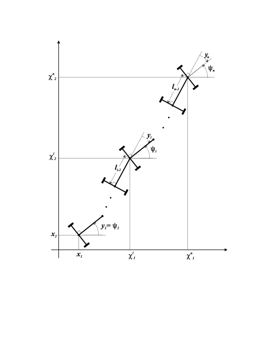
Figure 3: Kinematic scheme of a truck with multiple trailers.

The kinematic model of the system has the following form

$$\begin{array}[]{lll}\dot{x}_{1}&=&u_{1}\cos y_{1},\\ \dot{x}_{2}&=&u_{1}\sin y_{1},\\ \dot{y}_{i}&=&u_{1}\eta_{i}(y_{2},\ldots,y_{i+1}),\;i=1,\ldots,n-1,\\ \dot{y}_{n}&=&u_{2},\end{array}$$ (110)

where $\eta_{1}(y_{2})\!=\!l_{1}^{-1}\tan y_{2},\,\eta_{i}(y_{2},\ldots,y_{i+1})\!=\!(l_{i}^{-1}\tan y_{i+1}-l_{i-1}^{-1}\sin y_{i})\prod_{k=2}^{i}\sec y_{k},\,i\!=\!2,\ldots,n\!-\!1,$
$u_{1}$ is the longitudinal velocity of the first half-trailer, $u_{2}$ is the angular velocity of the truck forward axle spin with respect to the body of the truck. The equations (110) are derived in Appendix B. The system (110) is a special case of the system (6), (8) with $h_{1}=\mathop{\rm col}\nolimits(\eta_{1},\ldots,\eta_{n-1},0),\;\;h_{2}=\mathop{\rm col}\nolimits(0,\ldots,0,1).$

The system (110) is defined on the manifold $\mathcal{K}=\{q\in\mathcal{Q}\;|\;\cos y_{i}\not=0,\;i=2,\ldots,n\}.$ The kinematic model (110) is not defined when any two neighbor axles are orthogonal. When $n>1$ the manifold $\mathcal{K}$ is disconnected, being the union $\mathcal{K}=\bigcup_{\mu\in\mathrm{C}}\mathcal{M}_{\mu}$ of components $\mathcal{M}_{\mu}$ with the multi-index $\mu=(\mu_{1},\ldots,\mu_{n-1})$ taking on the values among the corners $\mathcal{C}$ of the $(n-1)$-dimensional cube, $\mathcal{C}=\{\mu\in R^{n-1}\;|\;\mu_{i}=0\mbox{\rm~{}or~{}}1,\;i=1,\ldots,n-1\}.$ Each $\mathcal{M}_{\mu},\;\mu\in\mathcal{C},$ is connected and has the form $\mathcal{M}_{\mu}=\{q\in\mathcal{Q}\;|\;\mu_{i-1}\pi-\pi/2<y_{i}<\mu_{i-1}\pi+\pi/2,\;i=2,\ldots,n\}.$ It should be noted that for $\mu\not=0$ the submanifold $\mathcal{M}_{\mu}$ includes exotic configurations with a neighbor half-trailers having the opposite orientation. The manifold $\mathcal{M}_{\mu}$ can be represented as $\mathcal{M}_{\mu}=R^{2}\times\mathcal{O}_{\mu},$ where $\mathcal{O}_{\mu}=\{y\in R\times S^{n-1}\;|\;\mu_{i-1}\pi-\pi/2<y_{i}<\mu_{i-1}\pi+\pi/2,\;i=2,\ldots,n\}.$ The metrics on the manifold $\mathcal{O}_{\mu},\;\mu\in\mathcal{C},$ is defined as $d(y^{\prime},y^{\prime\prime})=\sum_{i=1}^{n}|y^{\prime}_{i}-y^{\prime\prime}_{i}|.$

Proposition 4

: The system (110) satisfies the conditions of Theorem 3 on each manifold $\mathcal{M}_{\mu},\;\mu\in\mathcal{C}.$

The proof of Proposition 4 is given in Appendix C.

A corollary to Proposition 4 is the maneuverability of the system (110). It means that the midpoint of the tail-end axle of the vehicle that has $n-2$ trailers can trace any non-stop trajectory $x^{\mbox{\rm\tiny D}}\in C^{n+1}([0,\infty),R^{2})$ on the plane. This is a characteristic property of the smooth plane curves. It can be considered as a mechanical description of the smoothness of a planar curve.

According to Theorem 1, on each submanifold $\mathcal{M}_{\mu},\;\mu\in\mathcal{C},$ the system (110) has a set of maneuvering operators. Let us denote by $M^{+}_{\mu}$ the maneuvering operator, which results from choosing sign ”$+$” in (27) and choosing the value $s^{\mbox{\rm\tiny D}}_{1}(0)$ such that the inequality $-\pi<s^{\mbox{\rm\tiny D}}_{1}(0)\leq\pi$ in equation (29) holds. Similarly, by $M^{-}_{\mu}$ we denote the maneuvering operator, which results from ”$-$” in (27) and the value $s^{\mbox{\rm\tiny D}}_{1}(0)$ satisfying $0\leq s^{\mbox{\rm\tiny D}}_{1}(0)<2\pi.$ Then the operator $M^{+}_{\mu}$ defines the trajectory $q^{\mbox{\rm\tiny D}}$ for a forward motion of the tail-end trailer along the desired trajectory $x^{\mbox{\rm\tiny D}},$ and $M^{-}_{\mu}$ defines the trajectory $q^{\mbox{\rm\tiny D}}$ for a backward motion of the tail-end trailer along the same trajectory $x^{\mbox{\rm\tiny D}}.$

For each $\mu\in\mathcal{C}$ define the feedback function $\Phi_{\mu}$ on the manifold $\mathcal{M}_{\mu}$ using the formula (98). Now for any $\mu\in\mathcal{C}$ we construct the feedback operators $U^{+}_{\mu}$ and $U^{-}_{\mu}$ using the equations (38), (39) with $\Phi=\Phi_{\mu},$ $M=M^{+}_{\mu}$ and $M=M^{-}_{\mu}$ respectively. According to Theorem 3, the control laws $U^{+}_{\mu}$ and $U^{-}_{\mu}$ solve the problem of stabilizing the distinguished point trajectories of the system (110) on the manifold $\mathcal{M}_{\mu},\;\mu\in\mathcal{C}.$

Finally, we can design the feedback operators $U^{+}$ and $U^{-}$ on the manifold $\mathcal{K}=\bigcup_{\mu\in\mathcal{C}}\mathcal{M}_{\mu},$ using the formula (41) and the operators $U^{+}_{\mu},U^{-}_{\mu},\;\mu\in\mathcal{C}.$ Since the configuration manifold $\mathcal{Q}$ is the closure of $\mathcal{K},$ both control laws $U^{+}$ and $U^{-}$ solve the problem of almost global stabilization of the distinguished point trajectories for the considered vehicle.

It follows from Remark 2 that for all $t\geq 0$ the operator $U^{+}$ defines the positive input $u_{1}(t)>0,$ and $U^{-}$ defines the negative input $u_{1}(t)<0.$ Thus, the control law $U^{+}$ ensures a forward motion of the tail-end trailer and $U^{-}$ ensures a backward motion of the tail-end trailer. The latter control law solves intuitively harder problem of stabilizing the road train reverse motion along the desired trajectory.

Notice that the input $u_{1}$ in the system (110) is the longitudinal velocity of the tail-end trailer. In practice, the speed of the vehicle is controlled by the speed of the rear-axle assembly of the truck. Denote this alternative input $\tilde{u}_{1}.$ It is straightforward to show that the values $u_{1}$ and $\widetilde{u}_{1}$ satisfy the equation $\tilde{u}_{1}=u_{1}\prod_{k=2}^{n-1}\sec y_{k}.\;$Using this equation it is possible to express the control law in terms of inputs $\tilde{u}_{1}$ and $u_{2}.$

Consider special cases of the system (110).

For $n=2$ the equations (110) coincide with the equations of automobile (10) that were considered in Section 2. The proposed control law solves the problem of almost global stabilization of an automobile motion along any non-stop trajectory that has three bounded derivatives.

For $n=1$ the system (110) takes the form

$$\begin{array}[]{lll}\dot{x}_{1}&=&u_{1}\cos y_{1},\\ \dot{x}_{2}&=&u_{1}\sin y_{1},\\ \dot{y}_{1}&=&u_{2}.\end{array}$$ (111)

and describes the kinematics of the Chaplygin sled [24]. Equations (111) are also used as the kinematic model of caterpillar vehicles, the lunar vehicle Lunohod, the experimental robot Hilare described in [30]. The kinematic model (111) is defined on the whole configuration manifold of the system $\mathcal{Q}=R^{3}.$ Consequently, the proposed control law globally stabilizes strongly admissible trajectories of the Chaplygin sled.

7.  Simulation.

For $n=1,2,3,4$ the rectilinear motion and the circular motion of the system (110) with the constructed control law was simulated. The results of simulation demonstrate the efficiency of proposed control law.

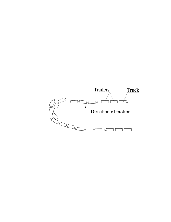
Figure 4: U-turn of the truck pushing two trailers in a backward direction.

As an illustration Fig. 4 shows the sequence of vehicle positions for an U-turn of the truck pushing two trailers in a backward direction. The desired trajectory corresponds to the motion along the dotted straight line. Animated results of this and some other experiments can be found in [9].

Appendix A. Proof of Proposition 1.

By virtue of K1 the system admits on the manifold $\mathcal{K}$ the kinematic model (2), and due to condition III for any $q=\mathop{\rm col}\nolimits(x,y)\in\mathcal{K}$ the vectorfields $g_{i},i=1,2,$ depend only on $y$-coordinates, i.e., $g_{i}(q)=g^{\prime}_{i}(y),i=1,2.$ Let $q=\mathop{\rm col}\nolimits(x,y)\in\mathcal{K}.$ Condition K2 implies the equalities $T_{q}(\mathcal{K})=R^{2}\times T_{y}(\mathcal{Y})$ and $g^{\prime}_{i}(y)=\mathop{\rm col}\nolimits(f^{\prime}_{i}(y),h^{\prime}_{i}(y)),\;i=1,2,$ where $f^{\prime}_{i}(y)\in R^{2},\;h^{\prime}_{i}(y)\in T_{y}(\mathcal{Y}).$ From the nonholonomic constraint (3) it follows that $f^{\prime}_{i}(y)=\lambda_{i}(y)f(y),i=1,2,$ where $\lambda_{i},i=1,2,$ are some functions defined on $\mathcal{Y},$ $f(y)=\mathop{\rm col}\nolimits(\cos y_{1},\sin y_{1}).$

Consider the feedback transformation

$$\left[\begin{array}[]{ccccccccccccccccccccc}\tilde{u}_{1}\\ \tilde{u}_{2}\end{array}\right]=\left[\begin{array}[]{ccccccccccccccccccccc}\lambda_{1},&\lambda_{2}\\ \lambda_{2},&-\lambda_{1}\end{array}\right]\left[\begin{array}[]{ccccccccccccccccccccc}u_{1}\\ u_{2}\end{array}\right].$$ (112)

Condition K3 implies that $\lambda_{1}^{2}(y)+\lambda_{2}^{2}(y)\not=0,$ i.e., the transformation (112) is nonsingular for all $y\in\mathcal{Y}.$ The transformation (112) brings the system (2) to the following form:

$$\begin{array}[]{lll}\dot{x}&=&\tilde{u}_{1}f(y),\\ \dot{y}&=&\tilde{u}_{1}h_{1}(y)+\tilde{u}_{2}h_{2}(y),\end{array}$$ (113)

where $h_{1}(y)=\lambda_{1}(y)h^{\prime}_{1}(y)+\lambda_{2}(y)h^{\prime}_{2}(y),\;h_{2}(y)=\lambda_{2}(y)h^{\prime}_{1}(y)-\lambda_{1}(y)h^{\prime}_{2}(y).$ Equations (113) differs from (6), (8) only by notation of inputs.

Appendix B. Derivation of the kinematic model for the truck with multiple trailers.

Let us introduce auxiliary variables: $\chi_{i}=(\chi^{1}_{i},\chi^{2}_{i})$ is the vector of the Cartesian coordinates of the $i$th axle midpoint, $\psi_{i}=\sum_{k=1}^{i}y_{k}$ is the heading angle of the $i$th pair of wheels, $\tau_{i}=(\cos\psi_{i},\sin\psi_{i})$ is the unit vector, that defines the orientation of the $i$th pair of wheels, $\nu_{i}=(-\sin\psi_{i},\cos\psi_{i})$ is the unit vector, that defines the orientation of the $i$th axle, $i=1,\ldots,n$ (see Fig. 3).

The nonslipping conditions for the wheels define the nonholonomic constraints

$$\langle\dot{\chi}_{i},\nu_{i}\rangle=0,\;\;i=1,\ldots,n.$$ (114)

In addition, the coordinates of the system satisfy the holonomic constraints

$$\chi_{i+1}=\chi_{i}+l_{i}\tau_{i},\;\;i=1,\ldots,n-1,$$ (115)

that describe the articulated joints of half-trailers. Here $l_{i}$ is the length of the $i$th half-trailer.

Differentiating (115), we obtain the equations

$$\dot{\chi}_{i+1}=\dot{\chi}_{i}+l_{i}\nu_{i}\dot{\psi}_{i},\;\;i=1,\ldots,n-1,$$ (116)

that can be used to exclude the derivatives of the dependent coordinates $\chi^{i},i=2,\ldots,n,$ from the equations (114). Thus, we deduce the equations of the nonholonomic constraints

$$-\sin\psi_{i}\dot{x}_{1}+\cos\psi_{i}\dot{x}_{2}+\sum_{j=1}^{i-1}l_{j}\cos(\psi_{j}-\psi_{i})\dot{\psi}_{j}=0,\;\;i=1,\ldots,n,$$ (117)

where $\chi^{1}=\mathop{\rm col}\nolimits(x_{1},x_{2})=x.$ The sum in the left-hand side of (117) is absent when $i=1.$

Let us show that the nonholonomic system described by the constraints (117) admits the kinematic model of the form (6), (8). Scalar multiplication of (116) by $\nu_{i}$ and $\tau_{i+1}$ gives the equations

$$\dot{\psi}_{i}=\upsilon_{i}l_{i}^{-1}\tan(\psi_{i+1}-\psi_{i}),\;i=1,\ldots,n-1,$$ (118)

$$\upsilon_{i+1}=\upsilon_{i}\sec(\psi_{i+1}-\psi_{i}),\;i=1,\ldots,n-1,$$ (119)

where $\upsilon_{i}=\langle\dot{\psi}_{i},\tau_{i}\rangle$ is the velocity of the $i$th half-trailer. Subject to the condition $\cos(\psi_{i+1}-\psi_{i})\not=0,\;i=1,\ldots,n-1,$ the equations (118), (119) yield the known equations of the truck with multiple trailers kinematics [23]

$$\begin{array}[]{lll}\dot{x}_{1}&=&\upsilon_{1}\cos\psi_{1},\\ \dot{x}_{2}&=&\upsilon_{1}\sin\psi_{1},\\ \dot{\psi}_{1}&=&\upsilon_{1}l_{1}^{-1}\tan(\psi_{2}-\psi_{1}),\\ \dot{\psi}_{i}&=&\upsilon_{1}l_{i}^{-1}\tan(\psi_{i+1}-\psi_{i})\prod_{k=2}^{i}\sec(\psi_{k}-\psi_{k-1}),\;i=2,\ldots,n-1,\\ \dot{\psi}_{n}&=&\upsilon_{n},\end{array}$$ (120)

where $\upsilon_{1}$ is the velocity of the tail-end half-trailer, $\upsilon_{n}$ is the angular velocity of the truck front axle spin with respect of the truck body. The conversion from the variables $\psi$ to the variables $y$ in (120) gives (110).

Appendix C. Proof of Proposition 3.

For fixed $\mu\in\mathcal{C}$ denote $S_{i}:\mathcal{O}_{\mu}\to R,i=1,\ldots,n,$ the $i$th component of the map $S,$ defined by (16). From the definition of the repeated Lie derivative it follows that for $i\geq 2$

$$\begin{array}[]{l}S_{i}(y)=L_{h_{1}}^{i-1}y_{1}=\sum_{j=1}^{n}\eta_{j}(y_{2},\ldots,y_{j+1})\displaystyle\frac{\partial}{\partial y_{j}}L_{h_{1}}^{i-2}y_{1}=\sum_{j=1}^{n}\eta_{j}(y_{2},\ldots,y_{j+1})\displaystyle\frac{\partial S_{i-1}(y)}{\partial y_{j}}.\end{array}$$ (121)

Let us show that

$$\frac{\partial S_{i}(y)}{\partial y_{j}}=0$$ (122)

for $i=1,\ldots,n,\;j=i+1,\ldots,n.$ To this end the equations

$$\begin{array}[]{l}\displaystyle\frac{\partial S_{i}(y)}{\partial y_{j}}=\sum_{\kappa=1}^{n}\displaystyle\frac{\partial}{\partial y_{j}}\eta_{\kappa}(y_{2},\ldots,y_{\kappa+1})\displaystyle\frac{\partial S_{i-1}(y)}{\partial y_{\kappa}}+\sum_{\kappa=1}^{n}\eta_{\kappa}(y_{2},\ldots,y_{\kappa+1})\displaystyle\frac{\partial}{\partial y_{\kappa}}\displaystyle\frac{\partial S_{i-1}(y)}{\partial y_{j}}\;,\;i\geq 2,\end{array}$$ (123)

are used that follow from (121). For $i=1$ $S_{1}(y)=y_{1},$ and (122) evidently holds. Suppose that (122) is fulfilled for $i-1,$ then the equation (123) implies $\displaystyle\frac{\partial S_{i}(y)}{\partial y_{j}}=0$ for $i<j\leq n.$ The equalities (122) are proved. From (122) it follows that $S_{i}(y)$ does not depend on $n$ and for $i\geq 2$

$$S_{i}(y)=\sum_{j=1}^{i-1}\eta_{j}(y_{2},\ldots,y_{j+1})\displaystyle\frac{\partial S_{i-1}(y)}{\partial y_{j}}.$$ (124)

The straightforward calculation gives

$$\begin{array}[]{l}\displaystyle\frac{\partial S_{i}(y)}{\partial y_{i}}=\sum_{\kappa=1}^{i-1}\displaystyle\frac{\partial}{\partial y_{i}}\eta_{\kappa}(y_{2},\ldots,y_{\kappa+1})\displaystyle\frac{\partial}{\partial y_{\kappa}}S_{i-1}(y)+\sum_{\kappa=1}^{i-1}\eta_{\kappa}(y_{2},\ldots,y_{\kappa+1})\displaystyle\frac{\partial}{\partial y_{\kappa}}\displaystyle\frac{\partial}{\partial y_{i}}S_{i-1}(y)=\\ \displaystyle\frac{\partial}{\partial y_{i}}\eta_{i-1}(y_{2},\ldots,y_{i})\displaystyle\frac{\partial}{\partial y_{i-1}}S_{i-1}(y)=l_{i-1}^{-1}\sigma_{i-1}(y_{2},\ldots,y_{i-1})\cos^{-2}(y_{i})\displaystyle\frac{\partial}{\partial y_{i-1}}S_{i-1}(y),\end{array}$$ (125)

where $\sigma_{1}\equiv 1,\;\sigma_{i}(y_{2},\ldots,y_{i})=\prod_{k=2}^{i}\sec(y_{k}),\ i=2\ldots,n.$

From (125) and the equality $\displaystyle\frac{\partial S_{1}(y)}{\partial y_{1}}=1$ it follows that for $i\geq 1$

$$\frac{\partial S_{i}(y)}{\partial y_{i}}=\sigma_{i}(y_{2},\ldots,y_{i})^{2}\prod_{j=1}^{i-1}\left[l_{j}^{-1}\sigma_{j}(y_{2},\ldots,y_{j})\right].$$ (126)

The equations (124) and (126) give for $i\geq 2$

$$S_{i}(y)=\theta_{i}(y_{2},\ldots,y_{i-1})\tan(y_{i})+\xi_{i}(y_{2},\ldots,y_{i-1}),$$ (127)

where

$$\begin{array}[]{l}\theta_{i}(y_{2},\ldots,y_{i-1})=\sigma_{i-1}(y_{2},\ldots,y_{i-1})^{2}\prod_{j=1}^{i-1}\left[l_{j}^{-1}\sigma_{j}(y_{2},\ldots,y_{j})\right],\\ \xi_{i}(y_{2},\ldots,y_{i-1})=-l_{i-1}^{-1}\sigma_{i-1}(y_{2},\ldots,y_{i-1})\tan(y_{i-1})+\sum_{j=1}^{i-2}\eta_{j}(y_{2},\ldots,y_{j+1})\displaystyle\frac{\partial S_{i-1}(y)}{\partial y_{j}}.\end{array}$$

From the definition of $S_{i}$ we have $L_{h_{2}}L_{h_{1}}^{i}y_{1}=\displaystyle\frac{\partial S_{i+1}}{\partial y_{n}}.$ This equality and the equations (122) and (126) imply that (13) and (14) are fulfilled for all $y\in\mathcal{O}_{\mu}.$

Let us show that $S$ maps bijectively $\mathcal{O}_{\mu}$ onto $R^{n}.$ Choose arbitrary $s^{*}\in R^{n}$ and consider the equation

$$s^{*}=S(y).$$ (128)

Define the vector $y^{*}\in\mathcal{O}_{\mu}$ by the recursive formulae

$$\begin{array}[]{l}y^{*}_{1}=s^{*}_{1},\\ y^{*}_{i}=\arctan(\frac{s^{*}_{i}-\xi_{i}(y^{*}_{1},\ldots,y^{*}_{i-1})}{\theta_{i}(y^{*}_{1},\ldots,y^{*}_{i-1})})+\mu_{i-1}\pi,\;i=2,\ldots,n.\end{array}$$

From (127) it is evidently follows that $y^{*}$ is a unique solution of (128).

We proved that the system (110) satisfies the conditions of Theorem 1.

Consider condition B of Theorem 3. Manifold $\mathcal{O}_{\mu}$ can be represented as $\mathcal{O}_{\mu}=R\times\check{\mathcal{O}}_{\mu},$ where $\check{\mathcal{O}}_{\mu}=\{\check{y}\in S^{n-1}\;|\;\mu_{i}\pi-\pi/2<\check{y}_{i}<\mu_{i}\pi+\pi/2,\;i=1,\ldots,n-1\}.$ On the manifold $\check{\mathcal{O}}_{\mu}$ define the metrics $\check{d}(\check{y}^{\prime},\check{y}^{\prime\prime})=\sum_{i=1}^{n-1}|\check{y}^{\prime}_{i}-\check{y}^{\prime\prime}_{i}|,$ then the metrics $d$ satisfies condition B of the theorem.

Condition C of the theorem evidently satisfied by the definition of the vectorfields $h_{1}$ and $h_{2}.$

Acknowledgment

The authors would like to thank B. D. Lubachevsky and I. V. Burkov for their thoughtful comments.

References

• [1] J. Ackermann, A. Bartlett, D. Kaesbauer, W. Sienel, and R. Steinhauser, Robust Constrol, Springer-Verlag, 1993.
• [2] A. M. Bloch, M. Reyhanoglu, and N. H. McClamroch, ”Control and stabilization of nonholonomic dynamical systems,” IEEE Trans. Automat. Contr., vol. 37, pp. 1746–1757, Nov. 1992.
• [3] R. W. Brockett, ”Asymptotic stability and feedback stabilization,” in Differential Geometric Control Theory, R. W. Brockett, R. S. Millmann, and H. J. Sussmann. Ed. Boston: Birkhäuser, 1983, pp. 181–191.
• [4] C. Canudas de Wit and O. J. Sordalen, ”Exponential stabilization of mobile robots with nonholonomic constraints,” IEEE Trans. Automat. Contr., vol. 37, pp. 1791–1797, Nov. 1992.
• [5] S. A. Chaplygin, ”Notes on theory of nonholonomic systems. Theorem on reducing factor,” Mathematical transactions, vol. 28, no. 2, 1911 (in Russian).
• [6] J. M. Coron, ”Global asymptotic stabilization for controllable systems without drift,” Mathematics of Control, Signals, and Systems, vol. 5, pp. 295–312, 1992.
• [7] M. Egerstedt, X. Hu, and A. Stotsky, ”Control of mobile platforms using virtual vehicle approach,” IEEE Trans. Automat. Contr., vol. 46, pp. 1777–1782, Nov. 2001.
• [8] A. L. Fradkov, S. V. Gusev, and I. A. Makarov, ”Robust speed-gradient adaptive control algorithms for manipulators and mobile robots,” in Proc. Conf. Decision Control, 1991, pp. 3095–3096.
• [9] S.V.Gusev, Sergei V. Gusev Web Page, at http://www.math.spbu.ru/user/gusev (web address is subject to change).
• [10] S. V. Gusev and I. A. Makarov, ”Stabilization of programmed motion of transport vechicle with a track-laying chassis,” Vestnik Leningradskogo Universiteta: Matematika, vol. 22, pp. 7–10, 1989.
• [11] S. V. Gusev and I. A. Makarov, ”An algorithm for stabilizing the program motion of transport robots,” Journal of computer and systems sciences international, vol. 35, no. 2, pp.155-163, 1994.
• [12] S. V. Gusev and I. A. Makarov, ”Motion control of maneuverable mobile robots,” deposited with VINITI, 2003 (in Russian).
• [13] S. V. Gusev, I. A. Makarov, I. E. Paromtchik, and V. A. Yakubovich, ”Adaptive stabilization of mechanical system with nonholonomic constraints,” in Proc. of 6th Intern. Symp. on Adaptive Systems Theory, St. Petersburg (Russia), 1999, pp. 101–104.
• [14] S. V. Gusev, I. A. Makarov, I. E. Paromtchik, V. A. Yakubovich, and C. Laugier, ”Adaptive motion control of a nonholonomic vehicle,” in Proc. IEEE Intern. Conference on Robotics and Automation, Leuven (Belgium), 1998, pp. 3285–3290.
• [15] A. Isidori, Nonlinear Control Systems, N. Y.: Springer-Verlag, 1995.
• [16] Z.-P. Jiang and H. Nijmeijer, ”A recursive technique for tracking control of nonholonomic systems in chained form,” IEEE Trans. Automat. Contr., vol. 44, pp. 265–279, Feb. 1999.
• [17] I. Kolmanovsky and N. H. McClamroch, ”Developments in nonholonomic control systems,” IEEE Control Systems Magazine, vol. 15, no. 6, pp. 20–36, 1995.
• [18] M. Krstic, I. Kanellakopoulos, and P. Kokotovic, Nonlinear and Adaptive Control Design, N. Y.: Willey-Interscience, 1995.
• [19] Z. X. Li and J. Canny, eds., Progress in nonholonomic motion planning, Kluwer, 1992.
• [20] I. A. Makarov, ”Desired trajectory tracking control for nonholonomic mechanical systems: a case study,” in Proc. 2nd European Control Conference, Groningen (The Netherlands), 1993, pp. 1444–1447.
• [21] B. M. Maschke and A. Van der Schaft, ”A hamiltonian approach to stabilization of nonholonomic mechanical systems,” in Proc. Conf. Decision Control, 1994, pp. 2950–2954.
• [22] R. T. M’Closkey and R. M. Murray, ”Exponential stabilization of driftless nonlinear control systems using homogeneous feedback,” IEEE Trans. Automat. Contr., vol. 42, pp. 614–628, May 1997.
• [23] R.M. Murray and S. S. Sastry, ”Nonholonomic motion planning: Steering using sinusoids,” IEEE Trans. Automat. Contr., vol. 38, pp. 700–716, May 1993.
• [24] Ju. I. Neimark and N. A. Fufaev, Dynamics of Nonholonomic Systems, vol. 33 of Translations of Mathematical Monographs, AMS, Providence, Rhode Island, 1972.
• [25] H. Nijmeijer and A. van der Schaft, Nonlinear Dynamical Control Systems, N.Y.: Springer-Verlag, 1990.
• [26] J.-P. Pomet, ”Explicit design of time-varying stabilizing control laws for a class of controllable systems without drift,” Syst. Control Lett., vol. 18, no. 2, pp. 147–158, 1992.
• [27] C. Samson, ”Control of chained systems: application to path following and time-varying point-stabilization of mobile robots,” IEEE Trans. Automat. Contr., vol. 40, pp. 64–77, Jan. 1995.
• [28] L. Schwartz, Mathematical analysis, Hermann, 1967 (in French).
• [29] O. J. Sordalen and O. Egeland, ”Exponential stabilization of nonholonomic chained systems,” IEEE Trans. Automat. Contr., vol. 40, pp. 35–49, Jan. 1995.
• [30] G. Walsh, D. Tilbury, S. Sastry, R. Murray, and J. P. Laumond, ”Stabilization of trajectories for systems with nonholonomic constraints,” IEEE Trans. Automat. Contr., vol. 39, pp. 216–222, Jan. 1994.