Computing Tropical Varieties

Abstract.

The tropical variety of a $d$-dimensional prime ideal in a polynomial ring with complex coefficients is a pure $d$-dimensional polyhedral fan. This fan is shown to be connected in codimension one. We present algorithmic tools for computing the tropical variety, and we discuss our implementation of these tools in the Gröbner fan software Gfan. Every ideal is shown to have a finite tropical basis, and a sharp lower bound is given for the size of a tropical basis for an ideal of linear forms.

1. Introduction

Every ideal in a polynomial ring with complex coefficients defines a tropical variety, which is a polyhedral fan in a real vector space. The objective of this paper is to introduce methods for computing this fan, which coincides with the “logarithmic limit set” in George Bergman’s seminal paper [2].

Given any polynomial $f\in\mathbb{C}[x_{1},x_{2},\ldots,x_{n}]$ and a vector $w\in\mathbb{R}^{n}$, the initial form ${\rm in}_{w}(f)$ is the sum of all terms in $f$ of lowest $w$-weight; for instance, if $\,\ell=x_{1}+x_{2}+x_{3}+1\,$ then $\,{\rm in}_{(0,0,1)}(\ell)\,=x_{1}+x_{2}+1\,$ and $\,{\rm in}_{(0,0,-1)}(\ell)\,=\,x_{3}$. The tropical hypersurface of $f$ is the set

$$\,\mathcal{T}(f)\quad=\,\quad\{\,w\in\mathbb{R}^{n}\,:\,{\rm in}_{w}(f)\,\,\,\hbox{is not a monomial}\,\}.$$

Equivalently, $\mathcal{T}(f)$ is the union of all codimension one cones in the inner normal fan of the Newton polytope of $f$. Note that $\mathcal{T}(f)$ is invariant under dilation, so we may specify $\mathcal{T}(f)$ by giving its intersection with the unit sphere. For the linear polynomial $\ell$ above, $\mathcal{T}(\ell)$ is a two-dimensional fan with six maximal cones. Its intersection with the $2$-sphere is the complete graph on the four nodes $(1,0,0)$, $(0,1,0)$, $(0,0,1)$ and $-(\frac{1}{\sqrt{3}},\frac{1}{\sqrt{3}},\frac{1}{\sqrt{3}})$.

A finite intersection of tropical hypersurfaces is a tropical prevariety [12]. If we pick the second linear form $\ell^{\prime}=x_{1}+x_{2}+2x_{3}$ then $\mathcal{T}(\ell^{\prime})$ is a graph with two vertices connected by three edges on the $2$-sphere, and $\,\mathcal{T}(\ell)\cap\mathcal{T}(\ell^{\prime})$ consists of three edges of $\mathcal{T}(\ell)$ which are adjacent to $-(\frac{1}{\sqrt{3}},\frac{1}{\sqrt{3}},\frac{1}{\sqrt{3}})$. In particular, the tropical prevariety $\,\mathcal{T}(\ell)\cap\mathcal{T}(\ell^{\prime})$ is not a tropical variety.

Tropical varieties are derived from ideals. Namely, if $I$ is an ideal in $\mathbb{C}[x_{1},\ldots,x_{n}]$ then its tropical variety $\mathcal{T}(I)$ is the intersection of the tropical hypersurfaces $\mathcal{T}(f)$ where $f$ runs over all polynomials in $I$. Theorem 2.9 below states that every tropical variety is actually a tropical prevariety, i.e., the ideal $I$ has a finite generating set $\{f_{1},f_{2},\ldots,f_{r}\}$ such that

$$\mathcal{T}(I)\quad=\quad\mathcal{T}(f_{1})\,\cap\,\mathcal{T}(f_{2})\,\cap\,\cdots\,\cap\mathcal{T}(f_{r})\,.$$

If this holds then $\{f_{1},f_{2},\ldots,f_{r}\}$ is called a tropical basis of $I$. For instance, our ideal $I=\langle\ell,\ell^{\prime}\rangle$ has the tropical basis $\,\{\,x_{1}+x_{2}+2x_{3},\,x_{1}+x_{2}+2,\,x_{3}-1\,\}$, and we find that its tropical variety consists of three points on the sphere:

$$\mathcal{T}(I)\,\,\,\,=\,\,\,\bigl{\{}(1,0,0),\,(0,1,0),\,-(\frac{1}{\sqrt{2}},\frac{1}{\sqrt{2}},0)\bigr{\}}.$$

Our main contribution is a practical algorithm, along with its implementation, for computing the tropical variety $\mathcal{T}(I)$ from any generating set of its ideal $I$. The emphasis lies on the geometric and algebraic features of this computation. We do not address issues of computational complexity, which have been studied by Theobald [19]. Our paper is organized as follows.

In Section 2 we give precise specifications of the algorithmic problems we are dealing with, including the computation of a tropical basis. We show that a finite tropical basis exists for every ideal $I$, and we give tight bounds on its size for linear ideals, thereby answering the question raised in [16, §5, page 13]. In Section 3 we prove that the tropical variety $\mathcal{T}(I)$ of a prime ideal $I$ is connected in codimension one. This result is the foundation of Algorithm 4.11 for computing $\mathcal{T}(I)$. Section 4 also describes methods for computing tropical bases and tropical prevarieties. Our algorithms have been implemented in the software package Gfan [9]. In Section 5 we compute the tropical variety of several non-trivial ideals using Gfan. The tropical variety $\mathcal{T}(I)$ is a subfan of the Gröbner fan of $I$ (defined in Section 2). The Gröbner fan is generally much more complicated and harder to compute than $\mathcal{T}(I)$. In Section 6 we compare these two fans, and we exhibit a family of curves for which the tropical variety of each member consists of four rays but the number of one-dimensional cones in the Gröbner fan grows arbitrarily.

A note on the choice of ground field is in order. In this paper we will work with varieties defined over $\mathbb{C}$. In the implementation of our algorithm (Section 5), we have required our polynomials to have rational coefficients, but our algorithms do not use any particular properties of $\mathbb{Q}$. It is important, however, that we work over a field of characteristic $0$, as our proof of correctness uses the Kleiman-Bertini theorem in the proof of Theorem 3.1.

In most papers on tropical algebraic geometry (cf. [5, 11, 12, 15, 19]), tropical varieties are defined from polynomials with coefficients in a field $K$ with a non-archimedean valuation. These tropical varieties are not fans but polyhedral complexes. We close the introduction by illustrating how our algorithms can be applied to this situation. Consider the field $\mathbb{C}(\epsilon)$ of rational functions in the unknown $\epsilon$. Then $\mathbb{C}(\epsilon)$ is a subfield of the algebraically closed field $\mathbb{C}\{\!\{\epsilon\}\!\}$ of Puiseux series with real exponents, which is an example of a field $K$ as in the above cited papers. Suppose we are given an ideal $I$ in $\mathbb{C}(\epsilon)[x_{1},\ldots,x_{n}]$. Let $I^{\prime}\subset\mathbb{C}\{\!\{\epsilon\}\!\}[x_{1},\ldots,x_{n}]$ be the ideal generated by $I$. The tropical variety $\mathcal{T}(I^{\prime})$, in the sense of the papers above, is a finite polyhedral complex in $\mathbb{R}^{n}$ which usually has both bounded and unbounded faces. To study this complex, we consider the polynomial ring in $n+1$ variables, $\,\mathbb{C}[\epsilon,x_{1},\ldots,x_{n}]\,$ and we let $J$ denote the intersection of $I$ with this subring of $\mathbb{C}(\epsilon)[x_{1}^{\pm},\ldots,x_{n}^{\pm}]$. Generators of $J$ are computed from generators of $I$ by clearing denominators and saturating with respect to $\epsilon$. The tropical variety of $I^{\prime}$ is related to the tropical variety of $J$ as follows.

Lemma 1.1.

A vector $w\in\mathbb{R}^{n}$ lies in the polyhedral complex $\mathcal{T}(I^{\prime})$ if and only if the vector $(1,w)\in\mathbb{R}^{n+1}$ lies in the polyhedral fan $\mathcal{T}(J)$.

Thus the tropical variety $\mathcal{T}(I^{\prime})$ equals the restriction of $\mathcal{T}(J)$ to the northern hemisphere of the $n$-sphere. Note that if $I$ is a prime ideal then so are $I^{\prime}$ and $J$. Einsiedler, Kapranov and Lind [5] have shown that if $I^{\prime}$ is prime, then $\mathcal{T}(I^{\prime})$ is connected. Our connectivity results in Section 3 (which use the result of [5]) imply the following result which was conjectured in [5].

Theorem 1.2.

If $I$ is an ideal in $\,\mathbb{C}\{\!\{\epsilon\}\!\}[x_{1},\ldots,x_{n}]$ whose radical is prime of dimension $d$, then the tropical variety $\mathcal{T}(I)$ is a pure $d$-dimensional polyhedral complex which is connected in codimension one.

On the algorithmic side, we conclude that the polyhedral complex $\mathcal{T}(I^{\prime})$ can be computed by restricting the flip algorithm of Section 4 to maximal cones in the fan $\mathcal{T}(J)$ which intersect the open northern hemisphere in $\mathbb{R}^{n+1}$.

2. Algorithmic Problems and Tropical Bases

For all algorithms in this paper we fix the ambient ring to be the polynomial ring over the complex numbers, $\mathbb{C}[\mathbf{x}]:=\mathbb{C}[x_{1},\ldots,x_{n}]$. The most basic computational problem in tropical geometry is the following:

Problem 2.1.

Given a finite list of polynomials $f_{1},\ldots,f_{r}\in\mathbb{C}[\mathbf{x}]$, compute the tropical prevariety $\mathcal{T}(f_{1})\cap\cdots\cap\mathcal{T}(f_{r})$ in $\mathbb{R}^{n}$ .

The geometry of this problem is best understood by considering the Newton polytopes ${\rm New}(f_{1}),\ldots,{\rm New}(f_{r})$ of the given polynomials. By definition, ${\rm New}(f_{i})$ is the convex hull in $\mathbb{R}^{n}$ of the exponent vectors which appear with non-zero coefficient in $f_{i}$. The tropical hypersurface $\mathcal{T}(f_{i})$ is the $(n-1)$-skeleton of the inner normal fan of the polytope ${\rm New}(f_{i})$. Our problem is to intersect these normal fans. The resulting tropical prevariety can be a fairly general polyhedral fan. Its maximal cones may have different dimensions.

The tropical variety of an ideal $I$ in $\mathbb{C}[\mathbf{x}]$ is the set $\mathcal{T}(I):=\bigcap_{f\in I}\mathcal{T}(f)$. Equivalently, $\mathcal{T}(I)=\{w\in\mathbb{R}^{n}\,:\,\textup{in}_{w}(I)\,\textup{does not contain a monomial}\}$ where $\textup{in}_{w}(I):=\langle\,\textup{in}_{w}(f)\,:\,f\in I\,\rangle$ is the initial ideal of $I$ with respect to $w$. Bieri and Groves [3] proved that $\mathcal{T}(I)$ is a $d$-dimensional fan when $d$ is the Krull dimension of $\mathbb{C}[\mathbf{x}]/I$. The fan is pure if $I$ is unmixed. In Section 3 we shall prove that $\mathcal{T}(I)$ is connected in codimension one if $I$ is prime.

We first note that it suffices to devise algorithms for computing tropical varieties of homogeneous ideals. Let ${}^{h}I\subset\mathbb{C}[x_{0},x_{1},\ldots,x_{n}]$ be the homogenization of an ideal $I$ in $\mathbb{C}[\mathbf{x}]$ and ${}^{h}f$ the homogenization of $f\in\mathbb{C}[\mathbf{x}]$.

Lemma 2.2.

Fix an ideal $I\subset\mathbb{C}[\mathbf{x}]$ and a vector $w\in\mathbb{R}^{n}$. The initial ideal ${\rm in}_{w}(I)$ contains a monomial if and only if ${\rm in}_{(0,w)}(^{h}I)$ contains a monomial.

Proof.

Suppose $\mathbf{x}^{\bf{u}}\in{\rm in}_{w}(I)$. Then $\mathbf{x}^{\bf{u}}={\rm in}_{w}(f)$ for some $f\in I$. The $(0,w)$-weight of a term in ${}^{h}f$ equals the $w$-weight of the corresponding term in $f$. Hence ${\rm in}_{(0,w)}(^{h}f)=x_{0}^{a}\mathbf{x}^{\bf{u}}\in{\rm in}_{(0,w)}(^{h}I)$ where $a$ is some non-negative integer.

Conversely, if $\mathbf{x}^{\bf{u}}\in{\rm in}_{(0,w)}(^{h}I)$ then $\mathbf{x}^{\bf{u}}={\rm in}_{(0,w)}(f)$ for some $f\in{}^{h}I$. Substituting $x_{0}=1$ in $f$ gives a polynomial in $I$. The $(0,w)$-weight of any term in $f$ equals the $w$-weight of the corresponding term in $\,f|_{x_{0}=1}$. Since ${\rm in}_{(0,w)}(f)$ is a monomial, only one term in $f$ has minimal $(0,w)$-weight. This term cannot be canceled during the substitution. Hence it lies in ${\rm in}_{w}(I)$. ∎

Our main goal in this paper is to solve the following problem.

Problem 2.3.

Given a finite list of homogeneous polynomials $f_{1},\ldots,f_{r}\in\mathbb{C}[\mathbf{x}]$, compute the tropical variety $\,\mathcal{T}(I)$ of their ideal $\,I=\langle f_{1},\ldots,f_{r}\rangle$.

It is important to note that the two problems stated so far are of a fundamentally different nature. Problem 2.1 is a problem of polyhedral geometry. It involves only polyhedral computations: no algebraic computations are required. Problem 2.3, on the other hand, combines the polyhedral aspect with an algebraic one. To solve Problem 2.3 we must perform algebraic operations (e.g. Gröbner bases) with polynomials. In Problem 2.1 we do not assume that the input polynomials $f_{1},\ldots,f_{r}$ are homogeneous as the polyhedral computations can be performed easily without this assumption.

Proposition 2.4.

Let $I$ be an ideal in $\mathbb{C}[\mathbf{x}]$ and let $w\in\mathbb{R}^{n}$. The following are equivalent:

1. The ideal $I$ is $w$-homogeneous; i.e. $I$ is generated by a set $S$ of $w$-homogeneous polynomials, meaning that $\textup{in}_{w}(f)=f$ for all $f\in S$.

2. The initial ideal $\textup{in}_{w}(I)$ is equal to $I$.

Proof.

If $I$ has a $w$-homogeneous generating set then $I\subseteq\textup{in}_{w}(I)$. Any maximal $w$-homogeneous component of $f\in I$ is in $I$. In particular $\textup{in}_{w}(f)\in I$. Conversely, the ideal $\textup{in}_{w}(I)$ is generated by $w$-homogeneous elements by definition so, if $I=\textup{in}_{w}(I)$, then $I$ is generated by $w$-homogeneous elements. ∎

The set of $w\in\mathbb{R}^{n}$ for which the above equivalent conditions hold is a vector subspace of $\mathbb{R}^{n}$. Its dimension is called the homogeneity of $I$ and is denoted ${\rm homog}(I)$. This space is contained in every cone of the fan $\mathcal{T}(I)$ and can be computed from the Newton polytopes of the polynomials that form any reduced Gröbner basis of $I$. Passing to the quotient of $\mathbb{R}^{n}$ modulo that subspace and then to a sphere around the origin, $\mathcal{T}(I)$ can be represented as a polyhedral complex of dimension $\,n-{\rm codim}(I)-{\rm homog}(I)-1={\rm dim}(I)-{\rm homog}(I)-1$. Here ${\rm codim}(I)$ and ${\rm dim}(I)$ are the codimension and dimension of $I$. In what follows, $\mathcal{T}(I)$ is always presented in this way, and every ideal $I$ is presented by a finite list of generators together with the three numbers $n$, ${\rm dim}(I)$ and ${\rm homog}(I)$.

Example 2.5.

Let $I$ denote the ideal which is generated by the $3\times 3$-minors of a symmetric $4\times 4$-matrix of unknowns. This ideal has $n=10$, ${\rm dim}(I)=7$ and ${\rm homog}(I)=4$. Hence $\mathcal{T}(I)$ is a two-dimensional polyhedral complex. We regard $\mathcal{T}(I)$ as the tropicalization of the secant variety of the Veronese threefold in $\mathbb{P}^{9}$, i.e., the variety of symmetric $4\times 4$-matrices of rank $\leq 2$, Applying our Gfan implementation (see Example 5.4), we find that $\mathcal{T}(I)$ is a simplicial complex consisting of $75$ triangles, $75$ edges and $20$ vertices. ∎

Our next problem concerns tropical bases. A finite set $\{f_{1},\ldots,f_{t}\}$ is a tropical basis of $I$ if $\,\langle f_{1},\ldots,f_{t}\rangle=I\,\,\textup{and}\,\,\mathcal{T}(I)=\mathcal{T}(f_{1})\cap\cdots\cap\mathcal{T}(f_{t}).$

Problem 2.6.

Compute a tropical basis of a given ideal $\,I\subset\mathbb{C}[\mathbf{x}]$.

A priori, it is not clear that every ideal $I$ has a finite tropical basis, but we shall prove this below. First, here is one case where this is easy:

Example 2.7.

If $\,I=\langle f\rangle\,$ is a principal ideal, then $\{f\}$ is a tropical basis. ∎

In [15] it was claimed that any universal Gröbner basis of $I$ is a tropical basis. Unfortunately, this claim is false as the following example shows.

Example 2.8.

Let $I$ be the intersection of the three linear ideals $\langle x+y,z\rangle$, $\langle x+z,y\rangle$, and $\langle y+z,x\rangle$ in $\mathbb{C}[x,y,z]$. Then $I$ contains the monomial $xyz$, so $\mathcal{T}(I)$ is empty. A minimal universal Gröbner basis of $I$ is

$$\mathcal{U}\quad=\quad\{\,x+y+z,\,x^{2}y+xy^{2},\,y^{2}z+yz^{2},\,x^{2}z+xz^{2}\,\},$$

and the intersection of the four corresponding tropical surfaces in $\mathbb{R}^{3}$ is the line $w_{1}=w_{2}=w_{3}$. Thus $\mathcal{U}$ is not a tropical basis of $I$. ∎

We now prove that every ideal $I\subset\mathbb{C}[\mathbf{x}]$ has a tropical basis. By Lemma 2.2, one tropical basis of a non-homogeneous ideal $I$ is the dehomogenization of a tropical basis for ${}^{h}I$. Hence we shall assume that $I$ is a homogeneous ideal.

Tropical bases can be constructed from the Gröbner fan of $I$ (see [13], [17]) which is a complete finite rational polyhedral fan in $\mathbb{R}^{n}$ whose relatively open cones are in bijection with the distinct initial ideals of $I$. Two weight vectors $w,w^{\prime}\in\mathbb{R}^{n}$ lie in the same relatively open cone of the Gröbner fan of $I$ if and only if ${\rm in}_{w}(I)={\rm in}_{w^{\prime}}(I)$. The closure of this cell, denoted by $C_{w}(I)$, is called a Gröbner cone of $I$. The $n$-dimensional Gröbner cones are in bijection with the reduced Gröbner bases, or equivalently, the monomial initial ideals of $I$. Every Gröbner cone of $I$ is a face of at least one $n$-dimensional Gröbner cone of $I$. If ${\rm in}_{w}(I)$ is not a monomial ideal, then we can refine $w$ to $\prec_{w}$ by breaking ties in the partial order induced by $w$ with a fixed term order $\prec$ on $\mathbb{C}[\mathbf{x}]$. Let $\mathcal{G}_{\prec_{w}}(I)$ denote the reduced Gröbner basis of $I$ with respect to $\prec_{w}$. The Gröbner cone of $\mathcal{G}_{\prec_{w}}(I)$, denoted by $C_{\prec_{w}}(I)$, is an $n$-dimensional Gröbner cone that has $C_{w}(I)$ as a face. The tropical variety $\mathcal{T}(I)$ consists of all Gröbner cones $C_{w}(I)$ such that ${\rm in}_{w}(I)$ does not contain a monomial. From the description of $\mathcal{T}(I)$ as $\,\bigcap_{f\in I}\mathcal{T}(f)\,$ it is clear that $\mathcal{T}(I)$ is closed. Thus we deduce that $\mathcal{T}(I)$ is a closed subfan of the Gröbner fan. This endows the tropical variety $\mathcal{T}(I)$ with the structure of a polyhedral fan.

Theorem 2.9.

Every ideal $I\subset\mathbb{C}[\mathbf{x}]$ has a tropical basis.

Proof.

Let $\mathcal{F}$ be any finite generating set of $I$ which is not a tropical basis. Pick a Gröbner cone $C_{w}(I)$ whose relative interior intersects $\,\cap_{f\in\mathcal{F}}\mathcal{T}(f)\,$ non-trivially and whose initial ideal $\,{\rm in}_{w}(I)\,$ contains a monomial $\mathbf{x}^{\bf m}$. Compute the reduced Gröbner basis $\mathcal{G}_{\prec_{w}}(I)$ for a refinement $\prec_{w}$ of $w$, and let $h$ be the normal form of $\mathbf{x}^{\bf m}$ with respect to $\mathcal{G}_{\prec_{w}}(I)$. Let $f:=\mathbf{x}^{\bf m}-h$. Since the normal form of $\mathbf{x}^{\bf m}$ with respect to $\mathcal{G}_{\prec}({\rm in}_{w}(I))=\{{\rm in}_{w}(g):g\in\mathcal{G}_{\prec_{w}}(I)\}$ is $0$ and $h$ is the normal form of $\mathbf{x}^{\bf m}$ with respect to $\mathcal{G}_{\prec_{w}}(I)$, every monomial occurring in $h$ has higher $w$-weight than $\mathbf{x}^{\bf m}$. Moreover, $h$ depends only on the reduced Gröbner basis $\mathcal{G}_{\prec_{w}}(I)$ and is independent of the particular choice of $w$ in $C_{w}(I)$. Hence for any $w^{\prime}$ in the relative interior of $C_{w}(I)$, we have $\mathbf{x}^{\bf m}={\rm in}_{w^{\prime}}(f)$. This implies that the polynomial $f:=\mathbf{x}^{\bf m}-h$ is a witness for the cone $C_{w}(I)$ not being in the tropical variety $\mathcal{T}(I)$.

We now add the witness $f$ to the current basis $\mathcal{F}$ and repeat the process. Since the Gröbner fan has only finitely many cones, this process will terminate after finitely many steps. It removes all cones of the Gröbner fan which violate the condition for $\mathcal{F}$ to be a tropical basis. ∎

We next show that tropical bases can be very large even for linear ideals. Let $I$ be the ideal in $\mathbb{C}[\mathbf{x}]$ generated by $d$ linear forms $\sum_{j=1}^{n}a_{ij}x_{j}$ where $i=1,\ldots,d$ and $(a_{ij})$ is an integer $d\times n$ matrix of rank $d$. The tropical variety $\mathcal{T}(I)$ depends only on the matroid associated with $I$, and it is known as the Bergman fan of that matroid. The results on the Bergman fan proved in [1, 18] imply that the circuits in $I$ form a tropical basis. A circuit of $I$ is a non-zero linear polynomial $f\in I$ of minimal support. The following result answers the question which was posed in [16, §5].

Theorem 2.10.

For any $1\leq d\leq n$, there is a linear ideal $I$ in $\mathbb{C}[x_{1},\ldots,x_{n}]$ such that any tropical basis of linear forms in $I$ has size at least $\frac{1}{n-d+1}{n\choose d}$.

Proof.

Suppose that all $d\times d$-minors of the coefficient matrix $(a_{ij})$ are non-zero. Equivalently, the matroid of $I$ is uniform. There are ${n\choose n-d+1}$ circuits in $I$, each supported on a different $(n-d+1)$-subset of $\{x_{1},\ldots,x_{n}\}$. Since the circuits form a tropical basis of $I$ and each circuit has support of size $n-d+1$, the tropical variety $\mathcal{T}(I)$ consists of all vectors $w\in\mathbb{R}^{n}$ whose smallest $d+1$ components are equal. The latter condition is necessary and sufficient to ensure that no single variable in a circuit becomes the initial form of the circuit with respect to $w$. Consider any vector $w\in\mathbb{R}^{n}$ satisfying

$$\,w_{i_{1}}=w_{i_{2}}=\cdots=w_{i_{d}}\,<\,{\rm min}\bigl{(}w_{j}\,:\,j\in\{1,\ldots,n\}\backslash\{i_{1},i_{2},\ldots,i_{d}\}\bigr{)}.$$

Since $w\not\in\mathcal{T}(I)$, any tropical basis of linear forms in $I$ contains an $f$ such that $\,{\rm in}_{w}(f)\in\{x_{i_{1}},\ldots,x_{i_{d}}\}$. This implies that $f$ is one of the $d$ circuits whose support contains the $n-d$ variables $\,x_{j}\,$ with $j\not\in\{i_{1},\ldots,i_{d}\}$. The support of each circuit has size $n-d+1$, hence contains $n-d+1$ distinct $(n-d)$-subsets. There are ${n\choose d}$ $\,(n-d)$-subsets of $\{x_{1},\ldots,x_{n}\}$ to be covered. Hence any tropical basis consisting of linear forms has size at least $\frac{1}{n-d+1}{n\choose d}$. ∎

Example 2.11.

Let $d=3,n=5$. The Bergman fan $\mathcal{T}(I)$ corresponds to the line in tropical projective $4$-space which consists of the five rays in the coordinate directions. We have $\,\frac{1}{n-d+1}{n\choose d}\,=\,10/3$. Hence this line is not a complete intersection of three tropical hyperplanes, but it requires four. ∎

3. Transversality and Connectivity

In this section we assume that $I$ is a prime ideal of dimension $d$ in $\mathbb{C}[x_{1},\ldots,x_{n}]$. Then its tropical variety $\mathcal{T}(I)$ is called irreducible. It is a subfan of the Gröbner fan of $I$ and, by the Bieri-Groves Theorem [3, 18], all facets of $\mathcal{T}(I)$ are cones of dimension $d$. A cone of dimension $d-1$ in $\mathcal{T}(I)$ is called a ridge of the tropical variety $\mathcal{T}(I)$. A ridge path is a sequence of facets $\,F_{1},F_{2},\ldots,F_{k}\,$ such that $F_{i}\cap F_{i+1}$ is a ridge for all $\,i\in\{1,2,\ldots,k-1\}$. Our objective is to prove the following result, which is crucial for the algorithms.

Theorem 3.1.

Any irreducible tropical variety $\mathcal{T}(I)$ is connected in codimension one, i.e., any two facets are connected by a ridge path.

The proof of this theorem will be based on the following important lemma.

Lemma 3.2.

(Transverse Intersection Lemma) Let $I$ and $J$ be ideals in $\mathbb{C}[x_{1},\ldots,x_{n}]$ whose tropical varieties $\mathcal{T}(I)$ and $\mathcal{T}(J)$ meet transversally at a point $w\in\mathbb{R}^{n}$. Then $w\in\mathcal{T}(I+J)$.

By “meet transversely” we mean that if $F$ and $G$ are the cones of $\mathcal{T}(I)$ and $\mathcal{T}(J)$ which contain $w$ in their relative interior, then $\mathbb{R}F+\mathbb{R}G=\mathbb{R}^{n}$.

This lemma implies that any transverse intersection of tropical varieties is a tropical variety. In particular, any transverse intersection of tropical hypersurfaces is a tropical variety, and such a tropical variety is defined by an ideal which is a complete intersection in the commutative algebra sense.

Corollary 3.3.

For any two ideals $I$ and $J$ in $\mathbb{C}[x_{1},\ldots,x_{n}]$ we have

$$\mathcal{T}(I+J)\quad\subseteq\quad\mathcal{T}(I)\,\cap\,\mathcal{T}(J).$$

Equality holds if the latter intersection is transverse at every point except the origin and the two fans meet in at least one point other than the origin.

Proof.

We have $\mathcal{T}(I)\cap\mathcal{T}(J)=\bigcap_{f\in I}\mathcal{T}(f)\cap\bigcap_{f\in J}\mathcal{T}(f)=\bigcap_{f\in I\cup J}\mathcal{T}(f)$. Clearly, this contains $\mathcal{T}(I+J)=\bigcap_{f\in I+J}\mathcal{T}(f)$. If $\mathcal{T}(I)$ and $\mathcal{T}(J)$ intersect transversally and $w$ is a point of $\mathcal{T}(I)\cap\mathcal{T}(J)$ other than the origin then the preceeding lemma tells us that $w\in\mathcal{T}(I+J)$. Thus $\mathcal{T}(I+J)$ contains every point of $\mathcal{T}(I)\cap\mathcal{T}(J)$ except possibly the origin. In particular, $\mathcal{T}(I+J)$ is not empty. Every nonempty fan contains the origin, so we see that the origin is in $\mathcal{T}(I+J)$ as well. ∎

We first derive Theorem 3.1 from Lemma 3.2, which will be proved later. We must at this point address an annoying technical detail. The subset $\mathcal{T}(I)\subset\mathbb{R}^{n}$ depends only on the ideal $I\mathbb{C}[\mathbf{x}^{\pm 1}]$ generated by $I$ in the Laurent polynomial ring $\mathbb{C}[x_{1}^{\pm},\ldots,x_{n}^{\pm 1}]$. (This is easy to see: if $I_{1}$ and $I_{2}$ generate the same ideal in $\mathbb{C}[\mathbf{x}^{\pm 1}]$ and $w\not\in\mathcal{T}(I_{1})$ then there is a polynomial $f\in I_{1}$ such that $\mathrm{in}_{w}(f)$ is a monomial. There is some monomial $m$ such that $mf\in I_{2}$, then $\mathrm{in}_{w}(mf)$ is a monomial and $w\not\in\mathcal{T}(I_{2})$.) From a theoretical perspective then, it would be better to directly work with ideals in $\mathbb{C}[\mathbf{x}^{\pm 1}]$. One reason is the availability the symmetry group ${\mathrm{G}L}_{n}(\mathbb{Z})$ of the multiplicative group of monomials. The action of this group transforms $\mathcal{T}(I)$ by the obvious action on $\mathbb{R}^{n}$. This symmetry will prove invaluable for simplifying the arguments in this section. Therefore, in this section, we will work with ideals in $\mathbb{C}[\mathbf{x}^{\pm 1}]$. Computationally, however, it is much better to deal with ideals in $\mathbb{C}[\mathbf{x}]$ as it is for such ideals that Gröbner basis techniques have been developed and this is the approach we take in the rest of the paper.

Note that, if $I\subset\mathbb{C}[\mathbf{x}]$ is prime then so is the ideal it generates in $\mathbb{C}[\mathbf{x}^{\pm 1}]$. We will signify an application of the ${\mathrm{G}L}_{n}(\mathbb{Z})$ symmetry by the phrase “making a multiplicative change of variables”. The polyhedral structure on $\mathcal{T}(I)$ induced by the Gröbner fan of $I$ may change under a multiplicative change of variables of $I\mathbb{C}[\mathbf{x}^{\pm}]$ in $\mathbb{C}[\mathbf{x}^{\pm 1}]$, but all of the properties of $\mathcal{T}(I)$ that are of interest to us depend only on the underlying point set.

Proof of Theorem 3.1. As discussed, we replace $I$ by the ideal it generates in $\mathbb{C}[\mathbf{x}^{\pm 1}]$ and, by abuse of notation, continue to denote this ideal as $I$. The proof is by induction on $d={\rm dim}(\mathcal{T}(I))$. If $d\leq 1$ then the statement is trivially true. We now explain why the result holds for $d=2$. By a multiplicative change of coordinates, it suffices to check that $\mathcal{T}(I)\cap\{x_{n}=1\}$ is connected. Let $K$ be the Puiseux series field over $\mathbb{C}$. Let $I^{\prime}\subset K[x_{1},\ldots,x_{n-1}]$ be the prime ideal generated by $I$ via the inclusion $\mathbb{C}[x_{n}]\to K$. By Lemma 1.1, the tropical variety of $I^{\prime}$ is $\mathcal{T}(I)\cap\{x_{n}=1\}$. In [5] it was shown that the tropical variety of $I^{\prime}$ is connected whenever $I^{\prime}$ is prime. We conclude that $\mathcal{T}(I)\cap\{x_{n}=1\}$ is connected, so our result holds for $d=2$.

We now suppose that $d\geq 3$. Let $F$ and $F^{\prime}$ be facets of $\mathcal{T}(I)$. We can find

$$H\quad=\quad\bigl{\{}\,(u_{1},\ldots,u_{n})\in\mathbb{R}^{n}\,:\,a_{1}u_{1}+\cdots+a_{n}u_{n}=0\,\bigr{\}}$$

such that $a_{1},\ldots,a_{n}$ are relatively prime integers, both $H\cap F$ and $H\cap F^{\prime}$ are cones of dimension $d-1$, and $H$ intersects every cone of $\mathcal{T}(I)$ except for the origin transversally. To see this, select rays $w$ and $w^{\prime}$ in the relative interiors of $F$ and $F^{\prime}$. By perturbing $w$ and $w^{\prime}$ slightly, we may arrange that the span of $w$ and $w^{\prime}$ does not meet any ray of $\mathcal{T}(I)$ – here it is important that $d\geq 3$. Now, taking $H$ to be the span of $w$, $w^{\prime}$ and a generic $(n-3)$-plane, we get that $H$ also does not contain any ray of $\mathcal{T}(I)$ and hence does not contain any positive dimensional face of $\mathcal{T}(I)$. So $H$ is transverse to $\mathcal{T}(I)$ everywhere except at the origin. Since $H\cap F$ and $H\cap F^{\prime}$ are positive-dimensional (as $d\geq 2$), the hyperplane $H$ does intersect $\mathcal{T}(I)$ at points other than just the origin. The hyperplane $H$ is the tropical hypersurface of a binomial, namely, $H=\mathcal{T}(\langle f_{u}\rangle)$, where

$$f_{u}\quad=\quad\prod_{i:a_{i}>0}(u_{i}x_{i})^{a_{i}}\,-\,\prod_{j:a_{j}<0}(u_{j}x_{j})^{-a_{j}},$$

and $\,u=(u_{1},u_{2},\ldots,u_{n})\,$ is an arbitrary point in the algebraic torus $(\mathbb{C}^{*})^{n}$. Our transversality assumption regarding $H$ and Lemma 3.2 imply that

(1) $$H\,\cap\,\mathcal{T}(I)\quad=\quad\mathcal{T}(\langle f_{u}\rangle)\,\cap\,\mathcal{T}(I)\quad=\quad\mathcal{T}\bigl{(}I+\langle f_{u}\rangle\bigr{)}.$$

Since $I$ is prime of dimension $d$, and $f_{u}\not\in I$, the ideal $\,I+\langle f_{u}\rangle\,$ has dimension $d-1$ by Krull’s Principal Ideal Theorem [6, Theorem 10.1]. If $\,I+\langle f_{u}\rangle\,$ were a prime ideal then we would be done by induction. Indeed, this would imply that there is a ridge path between the facets $H\cap F$ and $H\cap F^{\prime}$ in the $(d-1)$-dimensional tropical variety $(\ref{HcT})$. Since $d\geq 3$, the $(d-1)$- and $(d-2)$-dimensional faces of $H\cap\mathcal{T}(I)$ arise uniquely from the intersections of $H$ with $d$- and $(d-1)$-dimensional faces of $\mathcal{T}(I)$. Hence this path is also a ridge path considered as a path in $\mathcal{T}(I)$.

Let $V(J)$ denote the subvariety of the algebraic torus $(\mathbb{C}^{*})^{n}$ defined by an ideal $J\subset\mathbb{C}[x_{1}^{\pm 1},\ldots,x_{n}^{\pm 1}]$. The tropical variety in (1) depends only on the subvariety of $(\mathbb{C}^{*})^{n}$ defined by our ideal $\,I+\langle f_{u}\rangle$. This subvariety is

(2) $$V\bigl{(}I+\langle f_{u}\rangle\bigr{)}\quad=\quad V(I)\,\cap\,V(f_{u})\quad=\quad V(I)\,\cap\,u^{-1}\cdot V(f_{\bf 1}).$$

Here ${\bf 1}$ denotes the identity element of $(\mathbb{C}^{*})^{n}$. For generic choices of the group element $u\in(\mathbb{C}^{*})^{n}$, the intersection (2) is an irreducible subvariety of dimension $d-1$ in $(\mathbb{C}^{*})^{n}$. This follows from Kleiman’s version of Bertini’s Theorem [10, Theorem III.10.8], applied to the algebraic group $(\mathbb{C}^{*})^{n}$. Hence (1) is indeed an irreducible tropical variety of dimension $d-1$, defined by the prime ideal $I+\langle f_{u}\rangle$. This completes the proof by induction. ∎

Proof of Lemma 3.2: Again, we replace $I\subset\mathbb{C}[\mathbf{x}]$ by the ideal it generates in $\mathbb{C}[\mathbf{x}^{\pm 1}]$. Let $F$ be the cone of $\mathcal{T}(I)$ which contains $w$ in its relative interior and $G$ the cone of $\mathcal{T}(J)$ which contains $w$ in its relative interior. Our hypothesis is that $F$ and $G$ meet transversally at $w$, that is,

$$\mathbb{R}F\,+\,\mathbb{R}G\quad=\quad\mathbb{R}^{n}.$$

We claim that the ideal ${\rm in}_{w}(I)$ is homogeneous with respect to any weight vector $v\in\mathbb{R}F$ or, equivalently (see Proposition 2.4), that ${\rm in}_{v}({\rm in}_{w}(I))={\rm in}_{w}(I)$. According to Proposition 1.13 in [17], for $\epsilon$ a sufficiently small positive number, ${\rm in}_{w+\epsilon v}(I)={\rm in}_{v}({\rm in}_{w}(I))$. The vector $w+\epsilon v$ is in the relative interior of $F$ so ${\rm in}_{w+\epsilon v}(I)={\rm in}_{w}(I)$. By the same argument, the ideal ${\rm in}_{w}(J)$ is homogeneous with respect to any weight vector in $\mathbb{R}G$.

After a multiplicative change of variables in $\,\mathbb{C}[x_{1}^{\pm 1},\ldots,x_{n}^{\pm 1}]\,$ we may assume that $w=e_{1}$, $\,\mathbb{R}\{e_{1},e_{2},\ldots,e_{s}\}\subseteq\mathbb{R}F\,$ and $\,\mathbb{R}\{e_{1},e_{s+1},\ldots,e_{n}\}\subseteq\mathbb{R}G$. We change the notation for the variables as follows:

$$t=x_{1},\,y=(y_{2},\ldots,y_{s})=(x_{2},\ldots,x_{s}),\,\,z=(z_{s+1},\ldots,z_{n})=(x_{s+1},\ldots,x_{n}).$$

The homogeneity properties of the two initial ideals ensure that we can pick generators $f_{1}(z),\ldots,$ $f_{a}(z)\,$ for ${\rm in}_{w}(I)$ and generators $g_{1}(y),\ldots,g_{b}(y)$ for ${\rm in}_{w}(J)$. Since ${\rm in}_{w}(I)$ is not the unit ideal, the Laurent polynomials $f_{i}(z)$ have a common zero $Z=(Z_{s+1},\ldots,Z_{n})\in(\mathbb{C}^{*})^{n-s}$, and likewise the Laurent polynomials $g_{j}(y)$ have a common zero $Y=(Y_{2},\ldots,Y_{s})\in(\mathbb{C}^{*})^{s-1}$.

Next we consider the following general chain of inclusions of ideals:

(3) $${\rm in}_{w}(I)\,\cdot{\rm in}_{w}(J)\,\subseteq\,{\rm in}_{w}(I\cdot J)\,\subseteq\,{\rm in}_{w}(I\,\cap\,J)\,\subseteq\,{\rm in}_{w}(I)\,\cap\,{\rm in}_{w}(J).$$

The product of two ideals which are generated by (Laurent) polynomials in disjoint sets of variables equals the intersection of the two ideals. Since the set of $y$-variables is disjoint from the set of $z$-variables, it follows that the first ideal in (3) equals the last ideal in (3). In particular, we conclude that

(4) $${\rm in}_{w}(I\,\cap\,J)\quad=\quad{\rm in}_{w}(I)\,\cap\,{\rm in}_{w}(J).$$

We next claim that

(5) $${\rm in}_{w}(I\,+\,J)\quad=\quad{\rm in}_{w}(I)\,+\,{\rm in}_{w}(J).$$

The left hand side is an ideal which contains both ${\rm in}_{w}(I)$ and ${\rm in}_{w}(J)$, so it contains their sum. We must prove that the right hand side contains the left hand side. Consider any element $f+g\in I+J$ where $f\in I$ and $g\in J$. Let $\,f\,=\,f_{0}(y,z)+t\cdot f_{1}(t,y,z)\,$ and $\,g\,=\,g_{0}(y,z)+t\cdot g_{1}(t,y,z)$. We have the following representation for some integer $a\geq 0$ and non-zero polynomial $h_{0}$:

$$f+g\quad=\quad t^{a}\cdot h_{0}(y,z)+t^{a+1}\cdot h_{1}(t,y,z).$$

If $a=0$ then we conclude

$${\rm in}_{w}(f+g)\,\,=\,\,h_{0}(y,z)\,\,=\,\,f_{0}(y,z)+g_{0}(y,z)\,\,\in\,\,{\rm in}_{w}(I)+{\rm in}_{w}(J).$$

If $a\geq 1$ then $\,f_{0}\,=\,-g_{0}\,$ lies in $\,{\rm in}_{w}(I)\,\cap\,{\rm in}_{w}(J)$. In view of (4), there exists $\,p\in\,I\cap J\,\,$ with $\,f_{0}\,=\,-g_{0}\,=\,{\rm in}_{w}(p)$. Then $\,f+g=(f-p)+(g+p)\,$ and replacing $f$ by $(f-p)/t$ and $g$ by $(g+p)/t$ puts us in the same situation as before, but with $a$ reduced by $1$. By induction on $a$, we conclude that $\,{\rm in}_{w}(f+g)$ is in $\,{\rm in}_{w}(I)+{\rm in}_{w}(J)$, and the claim (5) follows.

For any constant $\,T\in\mathbb{C}^{*}$, the vector $\,(T,Y_{2},\ldots,Y_{s},Z_{s+1},\ldots,Z_{n})\,$ is a common zero in $(\mathbb{C}^{*})^{n}$ of the ideal (5). We conclude that $\,{\rm in}_{w}(I+J)\,$ is not the unit ideal, so it contains no monomial, and hence $w\in\mathcal{T}(I+J)$. ∎

4. Algorithms

In this section we describe algorithms for solving the computational problems raised in Section 2. The emphasis is on algorithms leading to a solution of Problem 2.3 for prime ideals, taking advantage of Theorem 3.1. Recall that we only need to consider the case of homogeneous ideals in $\mathbb{C}[\mathbf{x}]$.

In order to state our algorithms we must first explain how polyhedral cones and polyhedral fans are represented. A polyhedral cone is represented by a canonical minimal set of inequalities and equations. Given arbitrary defining linear inequalities and equations, the task of bringing these to a canonical form involves linear programming. Representing a polyhedral fan requires a little thought. We are rarely interested in all faces of all cones.

Definition 4.1.

A set $S$ of polyhedral cones in $\mathbb{R}^{n}$ is said to represent a fan $\mathcal{F}$ in $\mathbb{R}^{n}$ if the set of all faces of cones in $S$ is exactly $\mathcal{F}$.

A representation may contain non-maximal cones, but each cone is represented minimally by its canonical form. A Gröbner cone $C_{w}(I)$ is represented by the pair $(\mathcal{G}_{\prec_{w}}(\textup{in}_{w}(I)),\mathcal{G}_{\prec_{w}}(I))$ of marked reduced Gröbner bases, where $\prec$ is some globally fixed term order. In a marked Gröbner basis the initial terms are distinguished. The advantage of using marked Gröbner bases is that the weight vector ${w}$ need not be stored – we can deduce defining inequalities for its cone from the marked reduced Gröbner bases themselves, see Example 5.1. This is done as follows; see [17, proof of Proposition 2.3]:

Lemma 4.2.

Let $I\subset\mathbb{C}[\mathbf{x}]$ be a homogeneous ideal, $\prec$ a term order and ${w}\in\mathbb{R}^{n}$ a vector. For any other vector ${w}^{\prime}\in\mathbb{R}^{n}$:

$${w}^{\prime}\in C_{{w}}(I)\quad\Longleftrightarrow\quad\forall\,f\in\mathcal{G}_{\prec_{w}}(I):\,\textup{in}_{{w}}(\textup{in}_{{w}^{\prime}}(f))=\textup{in}_{{w}}(f).$$

Our first two algorithms perform polyhedral computations, and they solve Problem 2.1. By the support of a fan we mean the union of its cones. Recall that, for a polynomial $f$, the tropical hypersurface $\mathcal{T}(f)$ is the union of the normal cones of the edges of the Newton polytope $\textup{New}(f)$. The first algorithm computes these cones.

Algorithm 4.3.

Tropical Hypersurface
Input: $f\in\mathbb{C}[\mathbf{x}]$.
Output: A representation $S$ of a polyhedral fan whose support is $\mathcal{T}(f)$.
$\{$
     $S:=\emptyset$;
     For every vertex $v\in\textup{New}(f)$
     $\{$
          Compute the normal cone $C$ of $v$ in $\textup{New}(f)$;
          $S:=S\cup\{\textup{the facets of }C\}$;
     $\}$
$\}$

Let $\mathcal{F}_{1}$ and $\mathcal{F}_{2}$ be polyhedral fans in $\mathbb{R}^{n}$. Their common refinement is

$$\mathcal{F}_{1}\wedge\mathcal{F}_{2}:=\{C_{1}\cap C_{2}\}_{(C_{1},C_{2})\in\mathcal{F}_{1}\times\mathcal{F}_{2}}.$$

To compute a common refinement we simply run through all pairs of cones in the fan representations and bring their intersection to canonical form. The canonical form makes it easy to remove duplicates.

Algorithm 4.4.

Common Refinement
Input: Representations $S_{1}$ and $S_{2}$ for polyhedral fans $\mathcal{F}_{1}$ and $\mathcal{F}_{2}$.
Output: A representation $S$ for the common refinement $\mathcal{F}_{1}\wedge\mathcal{F}_{2}$.
$\{$
     $S:=\emptyset$;
     For every pair $(C_{1},C_{2})\in S_{1}\times S_{2}$
          $S:=S\cup\{C_{1}\cap C_{2}\}$;
$\}$

If refinements of more than two fans are needed, Algorithm 4.4 can be applied successively. Note that the intersection of the support of two fans is the support of the fans’ common refinement. Hence Algorithm 4.4 can be used for computing intersections of tropical hypersurfaces. This solves Problem 2.1, but the output may be a highly redundant representation.

Recall (from the proof of Theorem 2.9) that a witness $f\in I$ is a polynomial which certifies $\,\mathcal{T}(f)\cap\textup{rel int}(C_{w}(I))=\emptyset$. Computing witnesses is essential for solving Problems 2.3 and 2.6. The first step of constructing a witness is to check if the ideal $\textup{in}_{w}(I)$ contains monomials, and, if so, compute one such monomial. The check for monomial containment can be implemented by saturating the ideal with respect to the product of the variables (cf. [17, Lemma 12.1]). Knowing that the ideal contains a monomial, a simple way of finding one is to repeatedly reduce powers of the product of the variables by applying the division algorithm until the remainder is $0$.

Algorithm 4.5.

Monomial in Ideal
Input: A set of generators for an ideal $I\subset\mathbb{C}[\mathbf{x}]$.
Output: A monomial $m\in I$ if one exists, no otherwise.
$\{$
     If $((I:x_{1}\cdots x_{n}^{\infty})\not=\langle 1\rangle)$ return no;
     $m:=x_{1}\cdots x_{n}$;
     While $(m\not\in I)$ $\,m:=m\cdot x_{1}\cdots x_{n}$;
     Return $m$;
$\}$

Remark 4.6.

To pick the smallest monomial in $I$ with respect to a term order, we first compute the largest monomial ideal contained in $I$ using [14, Algorithm 4.2.2] and then pick the smallest monomial generator of this ideal.

Constructing a witness from a monomial was already explained in the proof of Theorem 2.9. We only state the input and output of this algorithm.

Algorithm 4.7.

Witness
Input: A set of generators for an ideal $I\subset\mathbb{C}[\mathbf{x}]$ and a vector ${w}\in\mathbb{R}^{n}$ with $\textup{in}_{w}(I)$ containing a monomial.
Output: A polynomial $f\in I$ such that the tropical hypersurface $\mathcal{T}(f)$ and the relative interior of $C_{w}(I)$ have empty intersection.

Combining Algorithm 4.5 and Algorithm 4.7 with known methods (e.g. [17, Algorithm 3.6]) for computing Gröbner fans, we can now compute the tropical variety $\mathcal{T}(I)$ and a tropical basis of $I$. This solves Problem 2.3 and Problem 2.6. This approach is not at all practical, as shown in Section 6.

We will present a practical algorithm for computing $\mathcal{T}(I)$ when $I$ is prime. An ideal $I\subset\mathbb{C}[\mathbf{x}]$ is said to define a tropical curve if $\textup{dim}(I)=1+\textup{homog}(I)$. Our problems are easier in this case because a tropical curve consists of only finitely many rays and the origin modulo the homogeneity space.

Algorithm 4.8.

Tropical Basis of a Curve
Input: A set of generators $\mathcal{G}$ for an ideal $I$ defining a tropical curve.
Output: A tropical basis $\mathcal{G}^{\prime}$ of $I$.
$\{$
     Compute a representation $S$ of $\bigwedge_{g\in\mathcal{G}}\mathcal{T}(g)$;
     For every $C\in S$
     $\{$
          Let ${w}$ be a generic relative interior point in $C$;
          If ($\textup{in}_{w}(I)$ contains a monomial)
               then add a witness to $\mathcal{G}$ and restart the algorithm;
     $\}$
     $\mathcal{G}^{\prime}:=\mathcal{G}$;
$\}$

Proof of correctness. The algorithm terminates because $I$ has only finitely many initial ideals and at least one is excluded in every iteration. If a vector ${w}$ passes the monomial test (which verifies $w\in\mathcal{T}(I)$) then $C$ has dimension $0$ or $1$ modulo the homogeneity space since we are looking at a curve and ${w}$ is generic in $C$. Any other relative interior point of $C$ would also have passed the monomial test. (This property fails in higher dimensions, when $\mathcal{T}(I)$ is no longer a tropical curve). Hence, when we terminate only points in the tropical variety are covered by $S$. Thus $\mathcal{G}^{\prime}$ is a tropical basis. ∎

In the curve case, combining Algorithms 4.3 and 4.4 with Algorithm 4.8 we get a reasonable method for solving Problem 2.3. This method is used as a subroutine in Algorithm 4.10 below. In the remainder of this section we concentrate on providing a better algorithm for Problem 2.3 in the case of a prime ideal. The idea is to use connectivity to traverse the tropical variety.

The next algorithm is an important subroutine for us. We only specify the input and output. This algorithm is one step in the Gröbner walk [4].

Algorithm 4.9.

Lift
Input: Marked reduced Gröbner bases $\mathcal{G}_{\prec^{\prime}}(I)$ and $\mathcal{G}_{\prec_{w}}(\textup{in}_{w}(I))$ where ${w}\in C_{\prec^{\prime}}(I)$ is an unspecified vector and $\prec$ and $\prec^{\prime}$ are unspecified term orders.
Output: The marked reduced Gröbner basis $\mathcal{G}_{\prec_{w}}(I)$.

We now suppose that $I$ is a monomial-free prime ideal with $d=\textup{dim}(I)$, and $\prec$ is a globally fixed term order. We first describe the local computations needed for a traversal of the $d$-dimensional Gröbner cones contained in $\mathcal{T}(I)$.

Algorithm 4.10.

Neighbors
Input: A pair $(\mathcal{G}_{\prec_{w}}(\textup{in}_{w}(I)),\mathcal{G}_{\prec_{w}}(I))$ such that $\textup{in}_{w}(I)$ is monomial-free and $C_{w}(I)$ has dimension $d$.
Output: The collection $N$ of pairs of the form $(\mathcal{G}_{\prec_{{w}^{\prime}}}(\textup{in}_{{w}^{\prime}}(I)),\mathcal{G}_{\prec_{{w}^{\prime}}}(I))$ where one ${w}^{\prime}$ is taken from the relative interior of each $d$-dimensional Gröbner cone contained in $\mathcal{T}(I)$ that has a facet in common with $C_{w}(I)$.
$\{$
     $N:=\emptyset$;
     Compute the set $\mathcal{F}$ of facets of $C_{w}(I)$;
     For each facet $F\in\mathcal{F}$
     $\{$
          Compute the initial ideal $J:=\textup{in}_{\bf{u}}(I)$
               where ${\bf{u}}$ is a relative interior point in $F$;
          Use Algorithm 4.8 and Algorithm 4.4 to produce a relative
               interior point ${\bf{v}}$ of each ray in the curve $\mathcal{T}(J)$;
          For each such ${\bf{v}}$
          $\{$
               Compute $(\mathcal{G}_{\prec_{{\bf{v}}}}(\textup{in}_{{\bf{v}}}(J)),\mathcal{G}_{\prec_{{\bf{v}}}}(J))=(\mathcal{G}_{\prec_{{\bf{v}}_{\bf{u}}}}(\textup{in}_{{\bf{v}}}(J)),\mathcal{G}_{\prec_{{\bf{v}}_{\bf{u}}}}(J))$;
               Apply Algorithm 4.9 to $\mathcal{G}_{\prec_{w}}(I)$ and $\mathcal{G}_{\prec_{{\bf{v}}_{\bf{u}}}}(J)$ to get $\mathcal{G}_{\prec_{{\bf{v}}_{\bf{u}}}}(I)$;
               $N:=N\cup\{(\mathcal{G}_{\prec_{{\bf{v}}_{\bf{u}}}}(\textup{in}_{{\bf{v}}}(J)),\mathcal{G}_{\prec_{{\bf{v}}_{\bf{u}}}}(I))\}$;
          $\}$
     $\}$
$\}$

Proof of correctness. Facets and relative interior points are computed using linear programming. Figure 1 illustrates the choices of vectors in the algorithm. The initial ideal $\textup{in}_{\bf{u}}(I)$ is homogeneous with respect to the span of $F$. Hence its homogeneity space has dimension $d-1$. The Krull dimension of $\mathbb{C}[\mathbf{x}]/\textup{in}_{\bf{u}}(I)$ is $d$. Hence $\textup{in}_{\bf{u}}(I)$ defines a curve and $\mathcal{T}(\textup{in}_{\bf{u}}(I))$ can be computed using Algorithm 4.8. The identity $\textup{in}_{\bf{v}}(\textup{in}_{\bf{u}}(I))=\textup{in}_{{\bf{u}}+\varepsilon{\bf{v}}}(I)$ for small $\varepsilon>0$, see [17, Proposition 1.13], implies that we run through all the desired $\textup{in}_{{w}^{\prime}}(I)$ where ${w}^{\prime}={\bf{u}}+\varepsilon{\bf{v}}$ for small $\varepsilon>0$. The lifting step can be carried out since ${\bf{u}}\in C_{\prec_{w}}(I)$. ∎

Figure 1. A projective drawing of the situation in Algorithm 4.10, with $\mathcal{T}(I)$ on the left and $\mathcal{T}(\textup{in}_{\bf{u}}(I))$ on the right.

Algorithm 4.11.

Traversal of an Irreducible Tropical Variety
Input: A pair $(\mathcal{G}_{\prec_{w}}(\textup{in}_{w}(I)),\mathcal{G}_{\prec_{w}}(I))$ such that $\textup{in}_{w}(I)$ is monomial free and $C_{w}(I)$ has dimension $d$.
Output: The collection $T$ of pairs of the form $(\mathcal{G}_{\prec_{{w}^{\prime}}}(\textup{in}_{{w}^{\prime}}(I)),\mathcal{G}_{\prec_{{w}^{\prime}}}(I))$ where one ${w}^{\prime}$ is taken from the relative interior of each $d$-dimensional Gröbner cone contained in $\mathcal{T}(I)$. The union of all the $C_{{w}^{\prime}}(I)$ is $\mathcal{T}(I)$.
$\{$
     $T:=\{(\mathcal{G}_{\prec_{w}}(\textup{in}_{w}(I)),\mathcal{G}_{\prec_{w}}(I))\}$;
     $Old:=\emptyset$;
     While ($T\not=Old$)
     $\{$
          $Old:=T$;
          $T:=T\cup\textup{Neighbors}(T)$;
     $\}$
$\}$

Proof of correctness. By $\textup{Neighbors}(T)$ we mean the union of all the output of Algorithm 4.10 applied to all pairs in $T$. The algorithm computes the connected component of the starting pair. Since $I$ is a prime ideal, Theorem 3.1 implies that the union of all the computed $C_{{w}^{\prime}}(I)$ is $\mathcal{T}(I)$. ∎

To use Algorithm 4.11 we must know a starting $d$-dimensional Gröbner cone contained in the tropical variety. One inefficient method for finding one would be to compute the entire Gröbner fan. Instead we currently use heuristics, which are based on the following probabilistic recursive algorithm:

Algorithm 4.12.

Starting Cone
Input: A marked reduced Gröbner basis $\mathcal{G}$ for an ideal $I$ whose tropical variety is pure of dimension $d=\textup{dim}(I)$. A term order $\prec$ for tie-breaking.
Output: Two marked reduced Gröbner bases:

• One for an initial ideal $\textup{in}_{{w}^{\prime}}(I)$ without monomials, where the homogeneity space of $\textup{in}_{{w}^{\prime}}(I)$ has dimension $d$. The term order is $\prec_{{w}^{\prime}}$.

• A marked reduced Gröbner basis for $I$ with respect to $\prec_{{w}^{\prime}}$.

$\{$
     If ($\textup{dim}(I)=\textup{homog}(I)$)
          Return $(\mathcal{G}_{\prec}(I),\mathcal{G}_{\prec}(I))$;
     If not
     $\{$
          Repeat
          $\{$
               Compute a random reduced Gröbner basis of $I$;
               Compute a random extreme ray ${w}$ of its Gröbner cone;
          $\}$
          Until ($\textup{in}_{w}(I)$ is monomial free);
          Compute $\mathcal{G}_{\prec_{w}}(I)$;
          $(\mathcal{G}_{Init},\mathcal{G}_{Full})$:= Starting Cone($\mathcal{G}_{\prec_{w}}(\textup{in}_{w}(I))$);
          Apply Algorithm 4.9 to $\mathcal{G}_{\prec_{w}}(I)$ and $\mathcal{G}_{Full}$
               to get a marked reduced Gröbner basis $\mathcal{G}^{\prime}$ for $I$;
          Return $(\mathcal{G}_{Init},\mathcal{G}^{\prime})$;
     $\}$
$\}$

5. Software and Examples

We implemented the algorithms of Section 4 in the software package Gfan [9]. Gfan uses the library cddlib [7] for polyhedral computations such as finding facets and extreme rays of cones and bringing cones to canonical form. We require our ideals to be generated by polynomials in $\mathbb{Q}[\mathbf{x}]$. Exact arithmetic is done with the library gmp [8]. This is needed both for polyhedral computations and for efficient arithmetic in $\mathbb{Q}[\mathbf{x}]$. In this section we illustrate the use of Gfan in computing various tropical varieties.

Example 5.1.

We consider the prime ideal $\,I\subset\mathbb{C}[a,b,c,d,e,f,g]\,$ which is generated by the $3\times 3$ minors of the generic Hankel matrix of size $4\times 4$:

$$\left(\begin{array}[]{cccc}a&b&c&d\\ b&c&d&e\\ c&d&e&f\\ d&e&f&g\\ \end{array}\right).$$

Its tropical variety is a $4$-dimensional fan in $\mathbb{R}^{7}$ with $2$-dimensional homogeneity space. Its combinatorics is given by the graph in Figure 2. To compute $\mathcal{T}(I)$ in Gfan, we write the ideal generators on a file hankel.in:

% more hankel.in
{-c^3+2*b*c*d-a*d^2-b^2*e+a*c*e,-c^2*d+b*d^2+b*c*e-a*d*e-b^2*f+a*c*f,
-c*d^2+c^2*e+b*d*e-a*e^2-b*c*f+a*d*f,-d^3+2*c*d*e-b*e^2-c^2*f+b*d*f,
-c^2*d+b*d^2+b*c*e-a*d*e-b^2*f+a*c*f,-c*d^2+2*b*d*e-a*e^2-b^2*g+a*c*g,
-d^3+c*d*e+b*d*f-a*e*f-b*c*g+a*d*g,-d^2*e+c*e^2+c*d*f-b*e*f-c^2*g+b*d*g,
-c*d^2+c^2*e+b*d*e-a*e^2-b*c*f+a*d*f,-d^3+c*d*e+b*d*f-a*e*f-b*c*g+a*d*g,
-d^2*e+2*c*d*f-a*f^2-c^2*g+a*e*g,-d*e^2+d^2*f+c*e*f-b*f^2-c*d*g+b*e*g,
-d^3+2*c*d*e-b*e^2-c^2*f+b*d*f,-d^2*e+c*e^2+c*d*f-b*e*f-c^2*g+b*d*g,
-d*e^2+d^2*f+c*e*f-b*f^2-c*d*g+b*e*g,-e^3+2*d*e*f-c*f^2-d^2*g+c*e*g}

We then run the command

gfan_tropicalstartingcone < hankel.in > hankel.start

which applies Algorithm 4.12 to produce a pair of marked Gröbner bases. This represents a maximal cone in $\mathcal{T}(I)$, as explained prior to Lemma 4.2.

% more hankel.start
{
c*f^2-c*e*g,
b*f^2-b*e*g,
b*e*f+c^2*g,
b*e^2+c^2*f,
b^2*g-a*c*g,
b^2*f-a*c*f,
b^2*e-a*c*e,
a*f^2-a*e*g,
a*e*f+b*c*g,
a*e^2+b*c*f}
{
c*f^2+e^3-2d*e*f+d^2*g-c*e*g,
b*f^2+d*e^2-d^2*f-c*e*f+c*d*g-b*e*g,
b*e*f+d^2*e-c*e^2-c*d*f+c^2*g-b*d*g,
b*e^2+d^3-2c*d*e+c^2*f-b*d*f,
b^2*g+c^2*e-b*d*e-b*c*f+a*d*f-a*c*g,
b^2*f+c^2*d-b*d^2-b*c*e+a*d*e-a*c*f,
b^2*e+c^3-2b*c*d+a*d^2-a*c*e,
a*f^2+d^2*e-2c*d*f+c^2*g-a*e*g,
a*e*f+d^3-c*d*e-b*d*f+b*c*g-a*d*g,
a*e^2+c*d^2-c^2*e-b*d*e+b*c*f-a*d*f}

Using Lemma 4.2 we can easily read off the canonical equations and equalities for the corresponding Gröbner cone $C_{w}(I)$. For example, the polynomials $cf^{2}-ceg$ and $cf^{2}+e^{3}-2def+d^{2}g-ceg$ represent the equation

$${w}_{c}+2{w}_{f}\,\,=\,\,{w}_{c}+{w}_{e}+{w}_{g}$$

and the inequalities

$${w}_{c}+2{w}_{f}\,\,\leq\,\,{\rm min}\bigl{\{}3{w}_{e},{w}_{d}+{w}_{e}+{w}_{f},2{w}_{d}+{w}_{g},{w}_{c}+{w}_{e}+{w}_{g}\bigr{\}}.$$

At this point, we could run Algorithm 4.11 using the following command:

gfan_tropicaltraverse < hankel.start > hankel.out

However, we can save computing time and get a better idea of the structure of $\mathcal{T}(I)$ by instructing Gfan to take advantage of symmetries of $I$ as it produces cones. The only symmetries that can be used in Gfan are those that simply permute variables. The output will show which cones of $\mathcal{T}(I)$ lie in the same orbit under the action of the symmetry group we provide.

Our ideal $I$ is invariant under reflecting the $4\times 4$-matrix along the anti-diagonal. This reverses the variables $a,b,\ldots,g$. To specify this permutation, we add the following line to the bottom of the file hankel.start:

{(6,5,4,3,2,1,0)}

We can add more symmetries by listing them one after another, separated by commas, inside the curly braces. Gfan will compute and use the group generated by the set of permutations we provide, and it will return an error if we input any permutation which does not keep the ideal invariant.

After adding the symmetries, we run the command

gfan_tropicaltraverse --symmetry < hankel.start > hankel.out

to compute the tropical variety. We show the output with some annotations:

% more hankel.out

Ambient dimension: 7
Dimension of homogeneity space: 2
Dimension of tropical variety: 4
Simplicial: true
Order of input symmetry group: 2
F-vector: (16,28)

A short list of basic data: the dimensions of the ambient space, of $\mathcal{T}(I)$, and of its homogeneity space, and also the face numbers ($f$-vector) of $\mathcal{T}(I)$ and the order of symmetry group specified in the input.

Modulo the homogeneity space:
{(6,5,4,3,2,-1,0),
 (5,4,3,2,1,0,-1)}

A basis for the homogeneity space. The rays are considered in the quotient of $\mathbb{R}^{7}$ modulo this $2$-dimensional subspace.

Rays:
{0: (-1,0,0,0,0,0,0),
 1: (-5,-4,-3,-2,-1,0,0),
 2: (1,0,0,0,0,0,0),
 3: (5,4,3,2,1,0,0),
 4: (2,1,0,0,0,0,0),
 5: (4,3,2,1,0,0,0),
 6: (0,-1,0,0,0,0,0),
 7: (6,5,4,3,2,0,0),
 8: (3,2,1,0,0,0,0),
 9: (0,0,-1,0,0,0,0),
 10: (0,0,0,0,-1,0,0),
 11: (0,0,0,-1,0,0,0),
 12: (-6,-4,-3,-3,-1,0,0),
 13: (-3,-2,-2,-1,-1,0,0),
 14: (3,2,2,1,1,0,0),
 15: (3,2,2,0,1,0,0)}

The direction vectors of the tropical rays. Since the homogeneity space is positive-dimensional, the directions are not uniquely specified. For instance, the vectors $(-5,-4,-3,-2,-1,0,0)$ and $(0,0,0,0,0,0,-1)$ represent the same ray. Note that Gfan uses negated weight vectors.

Rays incident to each
dimension 2 cone:
{{2,6}, {3,7},
{2,4}, {3,5},
{4,9}, {5,10},
{4,8}, {5,8},
{8,11},
{0,12}, {1,12},
{0,1},
{1,6}, {0,7},
{1,9}, {0,10},
{0,13}, {1,13},
{6,14}, {7,14},
{9,13}, {10,13},
{6,10}, {7,9},
{6,7},
{11,12},
{11,15},
{14,15}}

The cones in $\mathcal{T}(I)$ are listed from highest to lowest dimension. Each cone is named by the set of rays on it. There are 28 two-dimensional cones, broken down into 11 orbits of size 2 and 6 orbits of size 1.

The further output, which is not displayed here, shows that the 16 rays break down into 5 orbits of size 2 and 6 orbits of size 1.

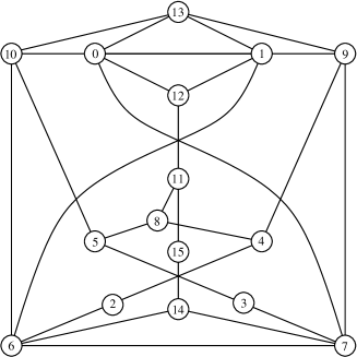
Figure 2. The tropical variety of the ideal generated by the $3\times 3$ minors of the generic $4\times 4$ Hankel matrix.

Using the same procedure, we now compute several more examples.

Example 5.2.

Let $I$ be the ideal generated by the $3\times 3$ minors of the generic $5\times 5$ Hankel matrix. We again use the symmetry group $\mathbb{Z}/2$. The tropical variety is a graph with vertex degrees ranging from 2 to 7.

Ambient dimension: 9
Dimension of homogeneity space: 2
Dimension of tropical variety: 4
Simplicial: true
F-vector: (28,53)

Example 5.3.

Let $I$ be the ideal generated by the $3\times 3$ minors of a generic $3\times 5$ matrix. We use the symmetry group $S_{5}\times S_{3}$, where $S_{5}$ acts by permuting the columns and $S_{3}$ by permuting the rows.

Ambient dimension: 15
Dimension of homogeneity space: 7
Dimension of tropical variety: 12
Simplicial: true
F-vector: (45,315,930,1260,630)

Example 5.4.

Let $I$ be the ideal generated by the $3\times 3$ minors of a generic $4\times 4$ symmetric matrix. We use the symmetry group $S_{4}$ which acts by simultaneously permuting the rows and the columns.

Ambient dimension: 10
Dimension of homogeneity space: 4
Dimension of tropical variety: 7
Simplicial: true
F-vector: (20,75,75)

If we take the $3\times 3$ minors of a generic $5\times 5$ symmetric matrix then we get

Ambient dimension: 15
Dimension of homogeneity space: 5
Dimension of tropical variety: 9
Simplicial: true
F-vector:    (75, 495, 1155, 855)

Example 5.5.

Let $I$ be the prime ideal of a pair of commuting $2\times 2$ matrices. That is, $I\subset\mathbb{C}[a,b,\ldots,h]$ is defined by the matrix equation

$$\left(\begin{array}[]{cc}a&c\\ b&d\end{array}\right)\left(\begin{array}[]{cc}e&g\\ f&h\end{array}\right)-\left(\begin{array}[]{cc}e&g\\ f&h\end{array}\right)\left(\begin{array}[]{cc}a&c\\ b&d\end{array}\right)=0.$$

The tropical variety is the graph $K_{4}$, which Gfan reports as follows:

Ambient dimension: 8
Dimension of homeogeneity space: 4
Dimension of tropical variety: 6
Simplicial: true
F-vector: (4,6)

If $I$ is the ideal of $3\times 3$ commuting symmetric matrices then we get:

Ambient dimension: 12
Dimension of homeogeneity space: 2
Dimension of tropical variety: 9
Simplicial: false
F-vector: (66,705,3246,7932,10888,8184,2745)

6. Tropical variety versus Gröbner fan

In this paper we developed tools for computing the tropical variety $\mathcal{T}(I)$ of a $d$-dimensional homogeneous prime ideal $I$ in a polynomial ring $\mathbb{C}[\mathbf{x}]$. We took advantage of the fact that, since $I$ is homogeneous, the set $\mathcal{T}(I)$ has naturally the structure of a polyhedral fan, namely, $\mathcal{T}(I)$ is the collection of all cones in the Gröbner fan of $I$ whose corresponding initial ideal is monomial-free. A naive algorithm would be to compute the Gröbner fan of $I$ and then retain only those $d$-dimensional cones who survive the monomial test (Algorithm 4.5). The software Gfan also computes the full Gröbner fan of $I$, and so we tested this naive algorithm. We found it to be too inefficient. The reason is that the vast majority of $d$-dimensional cones in the Gröbner fan of $I$ are typically not in the tropical variety $\mathcal{T}(I)$.

Example 6.1.

Consider the ideal $I$ in Example 5.1 which is generated by the $3\times 3$-minors of a generic $4\times 4$-Hankel matrix. Let $J={\rm in}_{w}(I)$ be its initial ideal with respect to the first vector $w$ in the list of rays. The initial ideal $J$ defines a tropical curve consisting of five rays and the origin. The curve is a subfan of the much more complicated Gröbner fan of $J$. The Gröbner fan is full-dimensional in $\mathbb{R}^{7}$ with $C_{0}(J)$ being three-dimensional. Its f-vector equals $(1,7167,32656,45072,19583)$. Of the $7167$ rays only $5$ are in the tropical variety. The Gröbner fan of $J$ is the link of the Gröbner fan of $I$ at $w$. We were unable to compute the full Gröbner fan of $I$.

Example 6.2.

Toric Ideals. Let $I=\langle\mathbf{x}^{\bf{u}}-\mathbf{x}^{\bf{v}}\,:\,A{\bf{u}}=A{\bf{v}}\rangle$ be the toric ideal of a matrix $A\in\mathbb{Z}^{d\times n}$ of rank $d$. The ideal $I$ is a prime of dimension $d$. The tropical variety $\mathcal{T}(I)$ coincides with the homogeneity space $C_{0}(I)$ which is just the row space of $A$. Hence $\mathcal{T}(I)$ modulo $C_{0}(I)$ is a single point. Yet, the Gröbner fan of $I$ can be very complicated, as it encodes the sensitivity information for an infinite family of integer programs [17, Chapter 7].

We next exhibit a family of ideals such that the number of rays in $\mathcal{T}(I)$ is constant while the number of rays in the Gröbner fan of $I$ grows linearly.

Theorem 6.3.

Fix $n\!=\!3,d\!=\!1$ and for any integer $p\geq 1$ consider the ideal

$$I_{p}\,\,\,=\,\,\,\langle\,\underline{x}-(z+1)^{p+2},\,\underline{y}-(z-1)^{p}\,\rangle.$$

Then $\mathcal{T}(I_{p})$ consists of $4$ rays but the Gröbner fan of $I_{p}$ has $\geq\frac{1}{4}(p+1)$ rays.

Sketch of proof: The ideal $I_{p}$ is prime. Its variety is the parametric curve $\,z\mapsto\bigl{(}(z+1)^{p+2},(z-1)^{p},z\bigr{)}$. The poles and zeros of this map are $0,-1,+1,\infty$. The tropical variety of $I_{p}$ consists of the four rays defined by the valuations at these points. These rays are generated by the columns of

$$\left(\begin{array}[]{cccc}0&0&p+2&-p-2\\ 0&p&0&-p\\ 1&0&0&-1\end{array}\right).$$

We examine the Gröbner fan around the ray $\,w=-(p+2,p,1)$. The initial ideal ${\rm in}_{w}(I_{p})$ equals the toric ideal $\,\langle x-z^{p+2},y-z^{p}\rangle$. To see this, we note that the two generators of $I_{p}$ form a Gröbner basis with respect to the underlined leading terms and ${\rm in}_{w}(I_{p})$ is generated by ${\rm in}_{w}(g)$ for each $g$ in this Gröbner basis since $w$ lies in this Gröbner cone. The Gröbner fan of ${\rm in}_{w}(I_{p})$ is the link at $w$ of the Gröbner fan of $I_{p}$. To prove the theorem we show that the Gröbner fan of ${\rm in}_{w}(I_{p})$ has at least $\frac{1}{2}(p+1)$ distinct Gröbner cones. This implies, by Euler’s formula, that the Gröbner fan of ${\rm in}_{w}(I_{p})$ has at least $\frac{1}{4}(p+1)$ rays and hence so does the Gröbner fan of $I_{p}$.

To argue that the Gröbner fan of ${\rm in}_{w}(I_{p})$ has at least $\frac{1}{2}(p+1)$ distinct Gröbner cones we use the methods in [17]. More specifically, this involves first showing that the binomials $g_{j}:=y^{j}-z^{p-2(j-1)}x^{j-1}$ for $j=1,\ldots,\frac{p+1}{2}$ are all in the universal Gröbner basis of ${\rm in}_{w}(I_{p})$. Each monomial in a binomial in the universal Gröbner basis of a toric ideal contributes a minimal generator to some initial ideal of the toric ideal. Thus there exist reduced Gröbner bases of ${\rm in}_{w}(I_{p})$ in which the binomials $g_{j}$ are elements with leading term $y^{j}$ for $j=1,\ldots,\frac{p+1}{2}$. This implies that these reduced Gröbner bases are all distinct, which completes the proof.

∎

While the Gröbner fan is a fundamental object which has had a range of applications (the Gröbner walk [4], integer programming (Example 6.2)), many computer algebra experts do not like it. Their view is that the Gröbner fan is a combinatorial artifact which is marginal to the real goal of computing the variety of $I$. While this opinion has some merit, the story is entirely different for the subfan $\mathcal{T}(I)$ of the Gröbner fan. In our view, the tropical variety is the variety of $I$. Every point on $\mathcal{T}(I)$ furnishes the starting system for a numerical homotopy towards the complex variety of $I$, see [18, Chapter 3]. Thus computing $\mathcal{T}(I)$ is not only much more efficient than computing the Gröbner fan of $I$, it is also geometrically more meaningful.

Acknowledgments. We thank Komei Fukuda for answering polyhedral computation questions and for customizing cddlib for our purpose, and we thank ETH Zürich for hosting Anders Jensen and Bernd Sturmfels during the summer of 2005. We acknowledge partial financial support by the University of Aarhus, the Danish Research Training Council (Forskeruddannelsesrådet, FUR), the Institute for Operations Research at ETH, the Swiss National Science Foundation Project 200021-105202, and the US National Science Foundation (DMS-0456960, DMS-0401047 and DMS-0354131).

Tristram Bogart, Department of Mathematics, University of Washington, Seattle, WA 98195-4350, USA, bogart@math.washington.edu.

Anders Jensen, Institut for Matematiske Fag, Aarhus Universitet, DK-8000 Århus, Denmark, ajensen@imf.au.dk.

David Speyer, Department of Mathematics, University of Michigan Ann Arbor, MI 48109-1043, USA, speyer@umich.edu.

Bernd Sturmfels, Department of Mathematics, University of California, Berkeley, CA 94720-3840, USA, bernd@math.berkeley.edu.

Rekha Thomas, Department of Mathematics, University of Washington, Seattle, WA 98195-4350, USA, thomas@math.washington.edu.

References

- [1] Federico Ardila and Caroline Klivans, The Bergman complex of a matroid and phylogenetic trees, math.CO/0311370, to appear in J. Combinatorial Theory Ser. B
- [2] George Bergman, The logarithmic limit set of an algebraic variety, Trans. Amer. Math. Soc. 157 (1971) 459–469.
- [3] Robert Bieri and John R.J. Groves, The geometry of the set of characters induced by valuations, J. Reine Angew. Mathematik 347 (1984) 168–195.
- [4] Stéphane Collart, Michael Kalkbrener and Daniel Mall, Converting bases with the Gröbner walk, J. Symbolic Computation 24 (1997) 465–469.
- [5] Manfred Einsiedler, Mikhail Kapranov and Douglas Lind, Non-archimedean amoebas and tropical varieties, to appear in J. Reine Angew. Mathematik.
- [6] David Eisenbud, Commutative Algebra with a View Toward Algebraic Geometry, Graduate Texts in Mathematics, 150. Springer-Verlag, New York, 1995
- [7] Komei Fukuda, cddlib reference manual, cddlib Version 093b. EPFL Lausanne and ETH Zürich, www.ifor.math.ethz.ch/~fukuda/cdd_home/cdd.htm.
- [8] Torbjorn Granlund et al, GNU Multiple Precision Arithmetic Library 4.1.4. September 2004. Available from http://swox.com/gmp/.
- [9] Anders Jensen, Gfan – a software system for Gröbner fans. Available at http://home.imf.au.dk/ajensen/software/gfan/gfan.html
- [10] Robin Hartshorne, Algebraic Geometry, Graduate Texts in Math., Springer, 1977.
- [11] Grigory Mikhalkin, Enumerative tropical algebraic geometry in , J. Amer. Math. Soc. 18 (2005) 313–377.
- [12] Jürgen Richter-Gebert, Bernd Sturmfels and Thorsten Theobald, First steps in tropical geometry, to appear in Idempotent Mathematics and Mathematical Physics, (eds. G.L. Litvinov and V.P. Maslov) American Math. Society, math.AG/0306366.
- [13] Teo Mora and Lorenzo Robbiano, The Gröbner fan of an ideal, Journal of Symbolic Computation 6 (1988) 183–208.
- [14] Mutsumi Saito, Bernd Sturmfels, and Nobuki Takayama, Gröbner Deformations of Hypergeometric Differential Equations, Springer-Verlag, 2000.
- [15] David Speyer and Bernd Sturmfels, The tropical Grassmannian, Advances in Geometry 4 (2004) 389–411.
- [16] David Speyer and Bernd Sturmfels, Tropical mathematics, Clay Institute lecture at Park City, Utah, July 2004, math.CO/0408099.
- [17] Bernd Sturmfels, Gröbner Bases and Convex Polytopes, University Lecture Series, American Math. Society, Providence, 1995.
- [18] Bernd Sturmfels, Solving System of Polynomial Equations, CBMS No. 97, American Math. Society, Providence, 2002.
- [19] Thorsten Theobald, On the frontiers of polynomial computations in tropical geometry, preprint, math.CO/0411012.