Optimal long term investment model
with memory

Abstract.

We consider a financial market model driven by an $\mathbf{R}^{n}$-valued Gaussian process with stationary increments which is different from Brownian motion. This driving noise process consists of $n$ independent components, and each component has memory described by two parameters. For this market model, we explicitly solve optimal investment problems. These include (i) Merton’s portfolio optimization problem; (ii) the maximization of growth rate of expected utility of wealth over the infinite horizon; (iii) the maximization of the large deviation probability that the wealth grows at a higher rate than a given benchmark. The estimation of paremeters is also considered.

1. Introduction

In this paper we study optimal investment problems for a financial market model with memory. This market model $\mathcal{M}$ consists of $n$ risky and one riskless assets. The price of the riskless asset is denoted by $S_{0}(t)$ and that of the $i$th risky asset by $S_{i}(t)$. We put $S(t)=(S_{1}(t),\dots,S_{n}(t))^{\prime}$, where $A^{\prime}$ denotes the transpose of a matrix $A$. The dynamics of the $\mathbf{R}^{n}$-valued process $S(t)$ are described by the stochastic differential equation

(1.1) $$\begin{split}dS_{i}(t)&=S_{i}(t)\left[\mu_{i}(t)dt+\sum\nolimits_{j=1}^{n}\sigma_{ij}(t)dY_{j}(t)\right],\quad t\geq 0,\\ \quad S_{i}(0)&=s_{i},\qquad\qquad\qquad\qquad\qquad\qquad\qquad i=1,\dots,n,\end{split}$$

while those of $S_{0}(t)$ by the ordinary differential equation

(1.2) $$dS_{0}(t)=r(t)S_{0}(t)dt,\quad t\geq 0,\quad S_{0}(0)=1,$$

where the coefficients $r(t)\geq 0$, $\mu_{i}(t)$, and $\sigma_{ij}(t)$ are continuous deterministic functions on $[0,\infty)$ and the initial prices $s_{i}$ are positive constants. We assume that the $n\times n$ volatility matrix $\sigma(t)=(\sigma_{ij}(t))_{1\leq i,j\leq n}$ is nonsingular for $t\geq 0$.

The major feature of the model $\mathcal{M}$ is the $\mathbf{R}^{n}$-valued driving noise process $Y(t)=(Y_{1}(t),\dots,Y_{n}(t))^{\prime}$ which has memory. We define the $j$th component $Y_{j}(t)$ by the autoregressive type equation

(1.3) $$\frac{dY_{j}(t)}{dt}=-\int_{-\infty}^{t}p_{j}e^{-q_{j}(t-s)}\frac{dY_{j}(s)}{ds}ds+\frac{dW_{j}(t)}{dt},\quad t\in\mathbf{R},\quad Y_{j}(0)=0,$$

where $W(t)=(W_{1}(t),\dots,W_{n}(t))^{\prime}$, $t\in\mathbf{R}$, is an $\mathbf{R}^{n}$-valued standard Brownian motion defined on a complete probability space $(\Omega,\mathcal{F},P)$, the derivatives $dY_{j}(t)/dt$ and $dW_{j}(t)/dt$ are in the random distribution sense, and $p_{j}$’s and $q_{j}$’s are constants such that

(1.4) $$0<q_{j}<\infty,\quad-q_{j}<p_{j}<\infty,\quad j=1,\dots,n$$

(cf. Anh and Inoue [1]). Equivalently, we may define $Y_{j}(t)$ by the moving-average type representation

(1.5) $$Y_{j}(t)=W_{j}(t)-\int_{0}^{t}\left[\int_{-\infty}^{s}p_{j}e^{-(q_{j}+p_{j})(s-u)}dW_{j}(u)\right]ds,\quad t\in\mathbf{R}$$

(see [1, Examples 2.12 and 2.14]). The components $Y_{j}(t)$, $j=1,\dots,n$, are Gaussian processes with stationary increments that are independent of each other. Each $Y_{j}(t)$ has short memory that is described by the two parameters $p_{j}$ and $q_{j}$. In the special case $p_{j}=0$, $Y_{j}(t)$ reduces to the Brownian motion $W_{j}(t)$. Driving noise processes with short or long memory of this kind are considered in [1], Anh et al. [2] and Inoue et al. [20], for the case $n=1$.

We define

$$\mathcal{F}_{t}:=\sigma\left(\sigma(Y(s):0\leq s\leq t)\cup\mathcal{N}\right),\quad t\geq 0,$$

where $\mathcal{N}$ is the $P$-null subsets of $\mathcal{F}$. This filtration $(\mathcal{F}_{t})_{t\geq 0}$ is the underlying information structure of the market model $\mathcal{M}$. From (1.5), we can easily show that $(Y(t))_{t\geq 0}$ is a semimartingale with respect to $(\mathcal{F}_{t})$ (cf. [1, Section 3]). In particular, we can interpret the stochastic differential equation (1.1) in the usual sense. In actual calculations, however, we need explicit semimartingale representations of $Y(t)$. It should be noticed that (1.5) is not a semimartingale representation of $Y(t)$ (except in the special case $p_{j}=0$). For, $W_{j}(t)$ involves the information of $Y_{j}(s)$ with $s<0$ and vice versa. The following two kinds of semimartingale representations of $Y(t)$ are obtained in [2, Example 5.3] and [20, Theorem 2.1], respectively:

(1.6) $$Y_{j}(t) =B_{j}(t)-\int_{0}^{t}\left[\int_{0}^{s}k_{j}(s,u)dY_{j}(u)\right]ds,\quad t\geq 0,\quad j=1,\dots,n,$$

(1.7) $$Y_{j}(t) =B_{j}(t)-\int_{0}^{t}\left[\int_{0}^{s}l_{j}(s,u)dB_{j}(u)\right]ds,\quad t\geq 0,\quad j=1,\dots,n,$$

where, for $j=1,\dots,n$, $(B_{j}(t))_{t\geq 0}$ is the so-called innovation process, i.e., an $\mathbf{R}$-valued standard Brownian motion such that

$$\sigma(Y_{j}(s):0\leq s\leq t)=\sigma(B_{j}(s):0\leq s\leq t),\quad t\geq 0.$$

Notice that $B_{j}$’s are independent of each other. The point of (1.6) and (1.7) is that the deterministic kernels $k_{j}(t,s)$ and $l_{j}(t,s)$ are given explicitly by

(1.8) $$k_{j}(t,s)=p_{j}(2q_{j}+p_{j})\frac{(2q_{j}+p_{j})e^{q_{j}s}-p_{j}e^{-q_{j}s}}{(2q_{j}+p_{j})^{2}e^{q_{j}t}-p_{j}^{2}e^{-q_{j}t}},\quad 0\leq s\leq t,$$

(1.9) $$l_{j}(t,s)=e^{-(p_{j}+q_{j})(t-s)}l_{j}(s),\quad 0\leq s\leq t,$$

with

(1.10) $$l_{j}(s):=p_{j}\left[1-\frac{2p_{j}q_{j}}{(2q_{j}+p_{j})^{2}e^{2q_{j}s}-p_{j}^{2}}\right],\quad s\geq 0.$$

We have the equalities

(1.11) $$\int_{0}^{t}k_{j}(t,s)dY_{j}(s)=\int_{0}^{t}l_{j}(t,s)dB_{j}(s),\quad t\geq 0,\quad j=1,\dots,n.$$

Many authors consider financial market models in which the standard driving noise, that is, Brownian motion, is replaced by a different one, such as fractional Brownian motion, so that the model can capture memory effect. To name some related contributions, let us mention here Comte and Renault [7, 8], Rogers [30], Heyde [16], Willinger et al. [32], Barndorff-Nielsen and Shephard [5], Barndorff-Nielsen et al. [4], Hu and Øksendal [18], Hu et al. [19], Elliott and van der Hoek [9], and Heyde and Leonenko [17]. In most of these references, driving noise processes are assumed to have stationary increments since this is a natural requirement of simplicity. Among such models, the above model $\mathcal{M}$ driven by $Y(t)$ which is a Gaussian process with stationary increments is possibly the simplest one. One advantage of $\mathcal{M}$ is that, by the semimartingale representations (1.6) and (1.7) of $Y(t)$, it admits explicit calculations in problems such as those considered in this paper. Another advantageous feature of the model $\mathcal{M}$ is that, assuming $\sigma_{ij}(t)=\sigma_{ij}$, real constants, we can easily estimate the characteristic parameters $p_{j}$, $q_{j}$ and $\sigma_{ij}$ from stock price data. We consider this parameter estimation in Appendix C.

For the market model $\mathcal{M}$, we consider an agent who has initial endowment $x\in(0,\infty)$ and invests $\pi_{i}(t)X^{x,\pi}(t)$ dollars in the $i$th risky asset for $i=1,\dots,n$ and $[1-\sum_{i=1}^{n}\pi_{i}(t)]X^{x,\pi}(t)$ dollars in the riskless asset at each time $t$, where $X^{x,\pi}(t)$ denotes the agent’s wealth at time $t$. The wealth process $X^{x,\pi}(t)$ is governed by the stochastic differential equation

(1.12) $$\frac{dX^{x,\pi}(t)}{X^{x,\pi}(t)}=\left[1-\sum\nolimits_{i=1}^{n}\pi_{i}(t)\right]\frac{dS_{0}(t)}{S_{0}(t)}+\sum\nolimits_{i=1}^{n}\pi_{i}(t)\frac{dS_{i}(t)}{S_{i}(t)},\quad X^{x,\pi}(0)=x.$$

Here, we choose the self-financing strategy $\pi(t)=(\pi_{1}(t),\dots,\pi_{n}(t))^{\prime}$ from the admissible class

$$\mathcal{A}_{T}:=\left\{\pi=(\pi(t))_{0\leq t\leq T}:\begin{split}&\mbox{$\pi$ is an $\mathbf{R}^{n}$-valued, progressively measurable}\\ &\mbox{process satisfying $\int_{0}^{T}\|\pi(t)\|^{2}dt<\infty$ a.s.}\end{split}\right\}$$

for the finite time horizon of length $T\in(0,\infty)$, where $\|\cdot\|$ denotes the Euclidean norm of $\mathbf{R}^{n}$. If the time horizon is infinite, we choose $\pi(t)$ from the class

$$\mathcal{A}:=\left\{(\pi(t))_{t\geq 0}:(\pi(t))_{0\leq t\leq T}\in\mathcal{A}_{T}\mbox{ for every }T\in(0,\infty)\right\}.$$

Let $\alpha\in(-\infty,1)\setminus\{0\}$ and $c\in\mathbf{R}$. In this paper, we consider the following three optimal investment problems for the model $\mathcal{M}$:

(P1) $$V(T,\alpha):=\sup_{\pi\in\mathcal{A}_{T}}\frac{1}{\alpha}E\left[(X^{x,\pi}(T))^{\alpha}\right],$$

(P2) $$J(\alpha):=\sup_{\pi\in\mathcal{A}}\limsup_{T\to\infty}\frac{1}{\alpha T}\log E\left[(X^{x,\pi}(T))^{\alpha}\right],$$

(P3) $$I(c):=\sup_{\pi\in\mathcal{A}}\limsup_{T\to\infty}\frac{1}{T}\log P\left[X^{x,\pi}(T)\geq e^{cT}\right].$$

The goal of Problem P1 is to maximize the expected utility of wealth at the end of the finite horizon. This classical optimal investment problem dates back to Merton [25]. We refer to Karatzas and Shreve [21] and references therein for work on this and related problems. In Hu et al. [19], this problem is solved for a Black–Scholes type model driven by fractional Brownian motion. In Section 2, assuming $p_{j}\geq 0$ for $j=1,\dots,n$, we explicitly solve this problem for the model $\mathcal{M}$. Our approach is based on a Cameron–Martin type formula which we prove in Appendix A. This formula holds under the assumption that a relevant Riccati type equation has a solution, and the key step of our arguments is to show the existence of such a solution (Lemma 2.1).

The aim of Problem P2 is to maximize the growth rate of expected utility of wealth over the infinite horizon. This problem is studied by Bielecki and Pliska [6], and subsequently by other authors under various settings, including Fleming and Sheu [11, 12], Kuroda and Nagai [22], Pham [28, 29], Nagai and Peng [27], Hata and Iida [13], and Hata and Sekine [14, 15]. In Section 3, we solve Problem P2 for the model $\mathcal{M}$ by verifying that a candidate of optimal strategy suggested by the solution to Problem P1 is actually optimal. In so doing, existence results on solutions to Riccati type equations (Lemmas 2.1 and 3.5) play a key role as in Problem P1. The result of Nagai and Peng [27] on the asymptotic behavior of solutions to Riccati equations, which we review in Appendix B, is also an essential ingredient in our arguments.

The purpose of Problem P3 is to maximize the large deviation probability that the wealth grows at a higher rate than the given benchmark $c$. This problem is studied by Pham [28, 29], in which a significant result, that is, a duality relation between Problems P2 and P3, is established. Subsequently, this problem is studied by Hata and Iida [13] and Hata and Sekine [14, 15] under different settings. In Section 4, we solve Problem P3 for the market model $\mathcal{M}$. In the approach of [28, 29], one needs an explicit expression of $J(\alpha)$. Since our solution to Problem P2 is explicit, we can solve Problem P3 for $\mathcal{M}$ using this approach. As in [28, 29], our solution to Problem 3 is given in the form of a sequence of nearly optimal strategies. For $c<\bar{c}$ with certain constant $\bar{c}$, an optimal strategy, rather than such a nearly optimal sequence, is obtained by ergodic arguments.

2. Optimal investment over the finite horizon

In this section, we consider the finite horizon optimization problem P1 for the market model $\mathcal{M}$. Throughout this section, we assume $\alpha\in(-\infty,1)\setminus\{0\}$ and

(2.1) $$0<q_{j}<\infty,\quad 0\leq p_{j}<\infty,\quad j=1,\dots,n.$$

Thus $p_{j}\geq 0$ rather than $p_{j}>-q_{j}$ (see Remark 2.6 below).

Let $Y(t)=(Y_{1}(t),\dots,Y_{n}(t))^{\prime}$ and $B(t)=(B_{1}(t),\dots,B_{n}(t))^{\prime}$ be the driving noise and innovation processes, respectively, described in Section 1. We define an $\mathbf{R}^{n}$-valued deterministic function $\lambda(t)=(\lambda_{1}(t),\dots,\lambda_{n}(t))^{\prime}$ by

(2.2) $$\lambda(t):=\sigma^{-1}(t)\left[\mu(t)-r(t)\mathbf{1}\right],\quad t\geq 0,$$

where $\mathbf{1}:=(1,\dots,1)^{\prime}\in\mathbf{R}^{n}$. For the kernels $k_{j}(t,s)$’s in (1.8), we put

$$k(t,s):=\mathrm{diag}(k_{1}(t,s),\dots,k_{n}(t,s)),\quad 0\leq s\leq t.$$

We denote by $\xi(t)=(\xi_{1}(t),\dots,\xi_{n}(t))^{\prime}$ the $\mathbf{R}^{n}$-valued process $\int_{0}^{t}k(t,s)dY(s)$, i.e.,

(2.3) $$\xi_{j}(t):=\int_{0}^{t}k_{j}(t,s)dY_{j}(s),\quad t\geq 0,\quad j=1,\dots,n.$$

By (1.1), (1.2), (1.6), and (1.12), the wealth process $X^{x,\pi}(t)$ evolves according to

$$\frac{dX^{x,\pi}(t)}{X^{x,\pi}(t)}=r(t)dt+\pi^{\prime}(t)\sigma(t)\left[\lambda(t)-\xi(t)\right]dt+\pi^{\prime}(t)\sigma(t)dB(t),\quad t\geq 0,$$

whence, by the Itô formula, we have, for $t\geq 0$,

(2.4) $$\begin{split}X^{x,\pi}(t)&=x\exp\left[\int_{0}^{t}\left\{r(s)+\pi^{\prime}(s)\sigma(s)\left(\lambda(s)-\xi(s)\right)-\frac{1}{2}\|\sigma^{\prime}(s)\pi(s)\|^{2}\right\}ds\right.\\ &\qquad\qquad\qquad\qquad\qquad\qquad\qquad+\left.\int_{0}^{t}\pi^{\prime}(s)\sigma(s)dB(s)\right].\end{split}$$

We define an $\mathbf{R}$-valued process $Z(t)$ by

$$Z(t):=\exp\left[-\int_{0}^{t}\left\{\lambda(s)-\xi(s)\right\}^{\prime}dB(s)-\frac{1}{2}\int_{0}^{t}\left\|\lambda(s)-\xi(s)\right\|^{2}ds\right],\quad t\geq 0.$$

Since $\lambda(t)-\xi(t)$ is a continuous Gaussian process, the process $Z(t)$ is a $P$-martingale (see, e.g., Example 3(a) in Liptser and Shiryayev [23, Section 6.2]). We define the $\mathbf{R}$-valued process $(\Gamma(t))_{0\leq t\leq T}$ by

$$\Gamma(t):=E\left[\left.Z^{\beta}(T)\right|\mathcal{F}_{t}\right],\quad 0\leq t\leq T,$$

where $\beta$ is the conjugate exponent of $\alpha$, i.e.,

$$(1/\alpha)+(1/\beta)=1.$$

Notice that $0<\beta<1$ (resp. $-\infty<\beta<0$) if $-\infty<\alpha<0$ (resp. $0<\alpha<1$). In view of Theorem 7.6 in Karatzas and Shreve [21, Chapter 3], to solve Problem P1, we only have to derive a stochastic integral representation for $\Gamma(t)$.

We define an $\mathbf{R}$-valued $P$-martingale $K(t)$ by

$$K(t):=\exp\left[-\beta\int_{0}^{t}\{\lambda(s)-\xi(s)\}^{\prime}dB(s)-\frac{\beta^{2}}{2}\int_{0}^{t}\|\lambda(s)-\xi(s)\|^{2}ds\right],\quad t\geq 0.$$

Then, by Bayes’ rule, we have

$$\begin{split}\Gamma(t)&=E\left[\left.K(T)\exp\left\{-\frac{1}{2}\beta(1-\beta)\int_{0}^{T}\|\lambda(s)-\xi(s)\|^{2}ds\right\}\right|\mathcal{F}_{t}\right]\\ &=K(t)\bar{E}\left[\left.\exp\left\{-\frac{1}{2}\beta(1-\beta)\int_{0}^{T}\|\lambda(s)-\xi(s)\|^{2}ds\right\}\right|\mathcal{F}_{t}\right]\end{split}$$

for $t\in[0,T]$, where $\bar{E}$ stands for the expectation with respect to the probability measure $\bar{P}$ on $(\Omega,\mathcal{F}_{T})$ such that $d\bar{P}/dP=K(T)$. Thus

(2.5) $$\begin{split}\Gamma(t)&=Z^{\beta}(t)\exp\left\{-\frac{1}{2}\beta(1-\beta)\int_{t}^{T}\|\lambda(s)\|^{2}ds\right\}\\ &\quad\times\bar{E}\left[\left.\exp\left\{-\frac{1}{2}\beta(1-\beta)\int_{t}^{T}\left(\|\xi(s)\|^{2}-2\lambda^{\prime}(s)\xi(s)\right)ds\right\}\right|\mathcal{F}_{t}\right].\end{split}$$

We are to apply Theorem A.1 in Appendix A to (2.5). By (1.11), the dynamics of $\xi(t)$ are described by the $n$-dimensional stochastic differential equation

(2.6) $$d\xi(t)=-(p+q)\xi(t)dt+l(t)dB(t),\quad t\geq 0,$$

where $p:=\mathrm{diag}(p_{1},\dots,p_{n})$, $q:=\mathrm{diag}(q_{1},\dots,q_{n})$, and $l(t):=\mathrm{diag}(l_{1}(t),\dots,l_{n}(t))$ with $l_{j}(t)$’s as in (1.10). Write $\bar{B}(t):=B(t)+\beta\int_{0}^{t}[\lambda(s)-\xi(s)]ds$ for $t\in[0,T]$. Then $\bar{B}(t)$ is an $\mathbf{R}^{n}$-valued standard Brownian motion under $\bar{P}$. By (2.6), the process $\xi(t)$ evolves according to

(2.7) $$d\xi(t)=\left[\rho(t)+b(t)\xi(t)\right]dt+l(t)d\bar{B}(t),\quad t\geq 0,$$

where $\rho(t)=(\rho_{1}(t),\dots,\rho_{n}(t))^{\prime}$, $b(t)=\mathrm{diag}(b_{1}(t),\dots,b_{n}(t))$ with

(2.8) $$\rho_{j}(t):=-\beta l_{j}(t)\lambda_{j}(t),\quad\quad t\geq 0,\quad j=1,\dots,n,$$

(2.9) $$b_{j}(t):=-(p_{j}+q_{j})+\beta l_{j}(t),\quad t\geq 0,\quad j=1,\dots,n.$$

By Theorem A.1 in Appendix A, we are led to consider the following one-dimensional backward Riccati equations: for $j=1,\dots,n$

(2.10) $$\dot{R}_{j}(t)-l_{j}^{2}(t)R_{j}^{2}(t)+2b_{j}(t)R_{j}(t)+\beta(1-\beta)=0,\quad 0\leq t\leq T,\quad R_{j}(T)=0.$$

The following lemma, especially (iii), is crucial in our arguments.

Lemma 2.1.

Let $j\in\{1,\dots,n\}$.

1. If $p_{j}=0$, then (2.10) has a unique solution $R_{j}(t)\equiv R_{j}(t;T)$.

2. If $-\infty<\alpha<0$, then (2.10) has a unique nonnegative solution $R_{j}(t)\equiv R_{j}(t;T)$.

3. If $p_{j}>0$ and $0<\alpha<1$, then (2.10) has a unique solution $R_{j}(t)\equiv R_{j}(t;T)$ such that $R_{j}(t)\geq b_{j}(t)/l_{j}^{2}(t)$ for $t\in[0,T]$.

Proof.

(i) If $p_{j}=0$, then (2.10) is linear, whence it has a unique solution.

(ii) If $-\infty<\alpha<0$, then $\beta(1-\beta)>0$, so that, by the well-known result on Riccati equations (see, e.g., Fleming and Rishel [10, Theorem 5.2] and Liptser and Shiryayev [23, Theorem 10.2]), (2.10) has a unique nonnegative solution.

(iii) When $p_{j}>0$ and $0<\alpha<1$, write

(2.11) $$a_{1}(t):=l_{j}^{2}(t),\quad a_{2}(t):=b_{j}(t),\quad a_{3}:=\beta(1-\beta),\quad t\geq 0.$$

Then the equation for $P(t):=R_{j}(t)-[a_{2}(t)/a_{1}(t)]$ becomes

(2.12) $$\dot{P}(t)-a_{1}(t)P^{2}(t)+a_{4}(t)=0,\quad 0\leq t\leq T,$$

where

$$a_{4}(t):=\frac{a_{2}^{2}(t)+a_{1}(t)a_{3}}{a_{1}(t)}+\frac{d}{dt}\left[\frac{a_{2}(t)}{a_{1}(t)}\right].$$

Since $dl_{j}(t)/dt>0$ and $\beta<0$, we see that

$$\frac{d}{dt}\left[\frac{a_{2}(t)}{a_{1}(t)}\right]=\frac{2(p_{j}+q_{j})-\beta l_{j}(t)}{l_{j}(t)^{3}}\cdot\frac{dl_{j}}{dt}(t)>0.$$

We write $a_{2}^{2}(t)+a_{1}(t)a_{3}$ as

$$(1-\beta)\left[(p_{j}+q_{j})^{2}-\{(p_{j}+q_{j})-l_{j}(t)\}^{2}\right]+[(p_{j}+q_{j})-l_{j}(t)]^{2},$$

which is positive since $0\leq l_{j}(t)\leq p_{j}$. Thus $a_{4}(t)>0$, so that (2.12) has a unique nonnegative solution $P(t)\equiv P(t;T)$. The desired solution to (2.10) is given by $R_{j}(t)=P(t)+[a_{2}(t)/a_{1}(t)]$. ∎

In what follows, we write $R_{j}(t)\equiv R_{j}(t;T)$ for the unique solution to (2.10) in the sense of Lemma 2.1. Then $R(t):=\mathrm{diag}(R_{1}(t),\dots,R_{n}(t))$ satisfies the backward matrix Riccati equation

(2.13) $$\begin{split}&\dot{R}(t)-R(t)l^{2}(t)R(t)+b(t)R(t)+R(t)b(t)+\beta(1-\beta)I_{n}=0,\quad 0\leq t\leq T,\\ &R(T)=0,\end{split}$$

where $I_{n}$ denotes the $n\times n$ unit matrix. For $j=1,\dots,n$, let $v_{j}(t)\equiv v_{j}(t;T)$ be the solution to the following one-dimensional linear equation:

(2.14) $$\begin{split}&\dot{v}_{j}(t)+[b_{j}(t)-l_{j}^{2}(t)R_{j}(t;T)]v_{j}(t)+\beta(1-\beta)\lambda_{j}(t)-R_{j}(t;T)\rho_{j}(t)=0,\\ &\quad 0\leq t\leq T,\quad v_{j}(T)=0.\end{split}$$

Then $v(t)\equiv v(t;T):=(v_{1}(t;T),\dots,v_{n}(t;T))^{\prime}$ satisfies the matrix equation

(2.15) $$\begin{split}&\dot{v}(t)+[b(t)-l^{2}(t)R(t;T)]v(t)+\beta(1-\beta)\lambda(t)-R(t;T)\rho(t)=0,\\ &\quad 0\leq t\leq T,\quad v(T)=0.\end{split}$$

We put, for $j=1,\dots,n$ and $(t,T)\in\Delta$,

(2.16) $$g_{j}(t;T):=v_{j}^{2}(t;T)l_{j}^{2}(t)+2\rho_{j}(t)v_{j}(t;T)-l_{j}^{2}(t)R_{j}(t;T)-\beta(1-\beta)\lambda_{j}^{2}(t),$$

where

(2.17) $$\Delta:=\{(t,T):0<T<\infty,\ 0\leq t\leq T\}.$$

We are now ready to give the desired representation for $\Gamma(t)$.

Proposition 2.2.

Write

(2.18) $$\psi(t):=\Gamma(t)\left[-\beta\lambda(t)+\{\beta-l(t)R(t;T)\}\xi(t)+l(t)v(t;T)\right],\quad 0\leq t\leq T.$$

Then, for $t\in[0,T]$, we have $\Gamma(t)=\Gamma(0)+\int_{0}^{t}\psi^{\prime}(s)dB(s)$ with

(2.19) $$\Gamma(0)=\exp\left[\frac{1}{2}\int_{0}^{T}\sum\nolimits_{j=1}^{n}g_{j}(s;T)ds\right].$$

Proof.

It follows from (2.5), (2.7), (2.13), (2.15) and Theorem A.1 that

(2.20) $$\Gamma(t)=Z^{\beta}(t)\exp\left[\sum_{j=1}^{n}\left\{v_{j}(t)\xi_{j}(t)-\frac{1}{2}\xi_{j}^{2}(t)R_{j}(t)+\frac{1}{2}\int_{t}^{T}g_{j}(s;T)ds\right\}\right].$$

The equality (2.19) follows from this. A straightforward calculation based on (2.20), (2.6) and the Itô formula gives $d\Gamma(t)=\psi^{\prime}(t)dB(t)$, where $\psi(t)$ is as in (2.18). Thus the proposition follows. ∎

Recall that we have assumed $\alpha\in(-\infty,1)\setminus\{0\}$ and (2.14). Here is the solution to Problem P1.

Theorem 2.3.

For $T\in(0,\infty)$, the strategy $(\hat{\pi}_{T}(t))_{0\leq t\leq T}\in\mathcal{A}_{T}$ defined by

(2.21) $$\hat{\pi}_{T}(t):=(\sigma^{\prime})^{-1}(t)\left[(1-\beta)\{\lambda(t)-\xi(t)\}-l(t)R(t;T)\xi(t)+l(t)v(t;T)\right]$$

is the unique optimal strategy for Problem P1. The value function $V(T)\equiv V(T,\alpha)$ in (P1) is given by

(2.22) $$V(T)=\frac{1}{\alpha}[xS_{0}(T)]^{\alpha}\exp\left[\frac{(1-\alpha)}{2}\sum\nolimits_{j=1}^{n}\int_{0}^{T}g_{j}(t;T)dt\right].$$

Proof.

By Theorem 7.6 in Karatzas and Shreve [21, Chapter 3], the unique optimal strategy $\pi_{T}(t)$ for Problem P1 is given by

$$\pi_{T}(t):=(\sigma^{\prime})^{-1}(t)\left[\Gamma^{-1}(t)\psi(t)+\lambda(t)-\xi(t)\right],\quad 0\leq t\leq T,$$

which, by (2.18), is equal to $\hat{\pi}_{T}(t)$. Thus the first assertion follows. By the same theorem in [21], $V(T)=\alpha^{-1}[xS_{0}(T)]^{\alpha}\Gamma^{1-\alpha}(0)$. This and (2.19) give (2.22). ∎

Remark 2.4.

We can regard $\xi(t)=\int_{0}^{t}k(t,s)dY(s)$, which is the only random term on the right-hand side of (2.21), as representing the memory effect. To illustrate this point, suppose that $(\sigma_{ij}(t))$ is a constant matrix. Then, by (C.2) in Appendix C, we can express $Y(t)$, whence $\xi(t)$, in terms of the past prices $S(u)$, $u\in[0,t]$, of the risky assets.

Remark 2.5.

From [21, Theorem 7.6], we also find that

$$X^{x,\hat{\pi}_{T}}(t)=x\frac{S_{0}(t)\Gamma(t)}{Z(t)\Gamma(0)},\quad 0\leq t\leq T.$$

Remark 2.6.

Regarding (2.1), we assume this to ensure the existence of solution to (2.10) for $j=1,\dots,n$. Under the weaker assumption (1.4), we could show by a different argument that, for $j=1,\dots,n$, (2.10) has a solution if $\alpha\in(-\infty,\bar{\alpha}_{j})\setminus\{0\}$, where $\bar{\alpha}_{j}\in(0,1]$ is defined by

$$\bar{\alpha}_{j}:=1\quad\mbox{if}\ 0\leq p_{j}<\infty,\quad:=\frac{(p_{j}+q_{j})^{2}}{l_{j}^{2}(0)+q_{j}^{2}}\quad\mbox{if}\ -q_{j}<p_{j}<0.$$

From this, we see that the same result as Theorem 2.3 holds under (1.4) if $-\infty<\alpha<\bar{\alpha}$, $\alpha\neq 0$, where $\bar{\alpha}:=\min\{\bar{\alpha}_{j}:j=1,\dots,n\}$. However, we did not succeed in extending the result to the most general case $-\infty<\alpha<1$, $\alpha\neq 0$. Such an extension, if possible, would lead us to the solution of Problem P3 under (1.4) (see Remark 3.8).

3. Optimal investment over the infinite horizon

In this section, we consider the infinite horizon optimization problem P2 for the financial market model $\mathcal{M}$. Throughout this section, we assume (2.1) and the following two conditions:

(3.1) $$\lim_{T\to\infty}\frac{1}{T}\int_{0}^{T}r(t)dt=\bar{r}\quad\mbox{with}\;\;\bar{r}\in[0,\infty),$$

(3.2) $$\lim_{t\to\infty}\lambda(t)=\bar{\lambda}\quad\mbox{with}\;\;\bar{\lambda}=(\bar{\lambda}_{1},\dots,\bar{\lambda}_{n})^{\prime}\in\mathbf{R}^{n}.$$

Here recall $\lambda(t)=(\lambda_{1}(t),\dots,\lambda_{n}(t))^{\prime}$ from (2.2). In the main result of this section (Theorem 3.4), we will also assume $\alpha^{*}<\alpha<1$, $\alpha\neq 0$, where

(3.3) $$\alpha^{*}:=\max(\alpha_{1}^{*},\dots,\alpha_{n}^{*})$$

with

(3.4) $$\alpha^{*}_{j}:=\left\{\begin{split}&-\infty\quad\mbox{if}\quad 0\leq p_{j}\leq 2q_{j},\\ &-3-\frac{8q_{j}}{p_{j}-2q_{j}}\quad\mbox{if}\quad 2q_{j}<p_{j}<\infty.\end{split}\right.$$

Notice that $\alpha^{*}\in[-\infty,-3)$.

To give the solution to Problem P2, we take the following steps:

1. For the value function $V(T)\equiv V(T,\alpha)$ in (P1), we calculate the following limit explicitly:

   (3.5) $$\tilde{J}(\alpha):=\lim_{T\to\infty}\frac{1}{\alpha T}\log[\alpha V(T)].$$

2. For $\hat{\pi}\in\mathcal{A}$ in (3.14) below, we calculate the growth rate

   (3.6) $$J^{*}(\alpha):=\lim_{T\to\infty}\frac{1}{\alpha T}\log E\left[(X^{x,\hat{\pi}}(T))^{\alpha}\right],$$

   and verify that $J^{*}(\alpha)=\tilde{J}(\alpha)$.

3. Since the definition of $V(T)$ implies

   (3.7) $$\limsup_{T\to\infty}\frac{1}{\alpha T}\log E[(X^{x,\pi}(T))^{\alpha}]\leq\tilde{J}(\alpha),\quad\forall\pi\in\mathcal{A},$$

   we conclude that $\hat{\pi}$ is an optimal strategy for Problem P2 and that the optimal growth rate $J(\alpha)$ in (P2) is given by $J(\alpha)=J^{*}(\alpha)=\tilde{J}(\alpha)$.

Let $\alpha\in(-\infty,1)\setminus\{0\}$ and $\beta$ be its conjugate exponent as in Section 2. For $j=1,\dots,n$, recall $b_{j}(t)$ from (2.9). We have $\lim_{t\to\infty}b_{j}(t)=\bar{b}_{j}$, where

$$\bar{b}_{j}:=-(1-\beta)p_{j}-q_{j}.$$

Notice that $\bar{b}_{j}<0$. We consider the equation

(3.8) $$p_{j}^{2}x^{2}-2\bar{b}_{j}x-\beta(1-\beta)=0.$$

When $p_{j}=0$, we write $\bar{R}_{j}$ for the unique solution $\beta(1-\beta)/(2q_{j})$ of this linear equation. If $p_{j}>0$, then

$$\bar{b}_{j}^{2}+\beta(1-\beta)p_{j}^{2}=(1-\beta)[(p_{j}+q_{j})^{2}-q_{j}^{2}]+q_{j}^{2}\geq q_{j}^{2}>0,$$

so that we may write $\bar{R}_{j}$ for the larger solution to the quadratic equation (3.8). Let

$$K_{j}:=\sqrt{\bar{b}_{j}^{2}+\beta(1-\beta)p_{j}^{2}}.$$

Then $\bar{b}_{j}-p_{j}^{2}\bar{R}_{j}=-K_{j}<0$.

As in Section 2, we write $R_{j}(t)\equiv R_{j}(t;T)$ for the unique solution to (2.10) in the sense of Lemma 2.1. Recall $\Delta$ from (2.17). The next proposition provides the necessary results on the asymptotic behavior of $R_{j}(t;T)$.

Proposition 3.1.

Let $-\infty<\alpha<1$, $\alpha\neq 0$, and $j\in\{1,\dots,n\}$. Then

1. $R_{j}(t;T)$ is bounded in $\Delta$.

2. $\lim_{T-t\to\infty,\ t\to\infty}R_{j}(t;T)=\bar{R}_{j}$.

3. For $\delta,\epsilon\in(0,\infty)$ such that $\delta+\epsilon<1$,

   $$\lim_{T\to\infty}\sup_{\delta T\leq t\leq(1-\epsilon)T}|R_{j}(t;T)-\bar{R}_{j}|=0.$$

Proof.

If $p_{j}=0$, then $l_{j}(t)=0$ and $b_{j}(t)=-q_{j}<0$ for $t\geq 0$, so that the assertions follow from Theorem B.3 in Appendix B.

We assume $p_{j}>0$. Since

$$|l_{j}(t)-p_{j}|\leq\frac{p_{j}^{2}}{2(p_{j}+q_{j})}e^{-2q_{j}t},\quad t\geq 0,$$

the function $l_{j}(t)$ converges to $p_{j}$ exponentially fast as $t\to\infty$. Hence the coefficients of the equation (2.10) converge to their counterparts in (3.8) exponentially fast, too. If $-\infty<\alpha<0$, then the desired assertions follow from Theorem B.1 in Appendix B (due to Nagai and Peng [27]). Suppose $0<\alpha<1$. Let $a_{1}(t)$, $a_{2}(t)$ and $a_{3}$ be as in (2.11). Since $R_{j}(t;T)\geq b_{j}(t)/l_{j}(t)^{2}$ and $b_{j}(t)/l_{j}(t)^{2}$ is bounded from below in $\Delta$, so is $R_{j}(t;T)$. To show that $R_{j}(t;T)$ is bounded from above in $\Delta$, we consider the solution $M_{j}(t)\equiv M_{j}(t;T)$ to the linear equation

$$\dot{M}_{j}(t)+2[a_{2}(t)-\bar{R}_{j}a_{1}(t)]M_{j}(t)+a_{3}+a_{1}(t)\bar{R}^{2}_{j}=0,\quad 0\leq t\leq T,\quad M_{j}(T)=0.$$

Since $M_{j}(T)-R_{j}(T)=0$ and

$$[\dot{M}_{j}(t)-\dot{R}_{j}(t)]+2[a_{2}(t)-\bar{R}_{j}a_{1}(t)][M_{j}(t)-R_{j}(t)]=-a_{1}(t)\left[R_{j}(t)-\bar{R}_{j}\right]^{2}\leq 0,$$

we have $R_{j}(t;T)\leq M_{j}(t;T)$ in $\Delta$. However, $a_{2}(t)-\bar{R}_{j}a_{1}(t)\to\bar{b}_{j}-\bar{R}_{j}\bar{p}_{j}^{2}<0$ as $t\to\infty$, so that $M_{j}(t;T)$ is bounded from above in $\Delta$, whence so is $R_{j}(t;T)$. The desired assertions now follow from Theorem B.2 in Appendix B. ∎

Let $j\in\{1,\dots,n\}$. For $\rho_{j}(t)$ in (2.8), we have $\lim_{t\to\infty}\rho_{j}(t)=\bar{\rho}_{j}$, where

$$\bar{\rho}_{j}:=-\beta p_{j}\bar{\lambda}_{j}.$$

Let $v_{j}(t)\equiv v_{j}(t;T)$ be the solution to (2.14) as in Section 2. Define $\bar{v}_{j}$ by

(3.9) $$\left(\bar{b}_{j}-p_{j}^{2}\bar{R}_{j}\right)\bar{v}_{j}+\beta(1-\beta)\bar{\lambda}_{j}-\bar{R}_{j}\bar{\rho}_{j}=0.$$

Proposition 3.2.

Let $-\infty<\alpha<1$, $\alpha\neq 0$, and $j\in\{1,\dots,n\}$. Then

1. $v_{j}(t;T)$ is bounded in $\Delta$.

2. $\lim_{T-t\to\infty,\ t\to\infty}v_{j}(t;T)=\bar{v}_{j}$.

3. For $\delta,\epsilon\in(0,\infty)$ such that $\delta+\epsilon<1$,

   $$\lim_{T\to\infty}\sup_{\delta T\leq t\leq(1-\epsilon)T}|v_{j}(t;T)-\bar{v}_{j}|=0.$$

Proof.

The coefficients of (2.14) converge to their counterparts in (3.9). Also,

$$\lim_{T-t\to\infty,\;t\to\infty}[b_{j}(t)-l_{j}^{2}(t)R_{j}(t;T)]=\bar{b}_{j}-p_{j}^{2}\bar{R}_{j}=-K_{j}<0.$$

Thus the proposition follows from Theorem B.3 in Appendix B. ∎

For $j=1,\dots,n$ and $-\infty<\alpha<1$, $\alpha\neq 0$, we put

(3.10) $$F_{j}(\alpha):=\frac{(p_{j}+q_{j})^{2}\bar{\lambda}_{j}^{2}\alpha}{\left[(1-\alpha)(p_{j}+q_{j})^{2}+\alpha p_{j}(p_{j}+2q_{j})\right]},$$

(3.11) $$\begin{split}&G_{j}(\alpha)\\ &\ \ :=(p_{j}+q_{j})-q_{j}\alpha-(1-\alpha)^{1/2}\left[(1-\alpha)(p_{j}+q_{j})^{2}+\alpha p_{j}(p_{j}+2q_{j})\right]^{1/2}.\end{split}$$

Recall the value function $V(T)\equiv V(T,\alpha)$ from (P1) and its representation (2.22). In the next proposition, we compute $\tilde{J}(\alpha)$ in (3.5).

Proposition 3.3.

Let $-\infty<\alpha<1$, $\alpha\neq 0$. Then the limit $\tilde{J}(\alpha)$ in (3.5) exists and is given by

(3.12) $$\tilde{J}(\alpha)=\bar{r}+\frac{(1-\alpha)}{2\alpha}\sum_{j=1}^{n}\bar{g}_{j},$$

where

$$\bar{g}_{j}:=\bar{v}^{2}_{j}p_{j}^{2}+2\bar{\rho}_{j}\bar{v}_{j}-p_{j}^{2}\bar{R}_{j}-\beta(1-\beta)\bar{\lambda}_{j}^{2},\quad j=1,\dots,n.$$

More explicitly,

(3.13) $$\tilde{J}(\alpha)=\bar{r}+\frac{1}{2\alpha}\sum_{j=1}^{n}F_{j}(\alpha)+\frac{1}{2\alpha}\sum_{j=1}^{n}G_{j}(\alpha).$$

Proof.

Recall $g_{j}(t;T)$ from (2.16). By Propositions 3.1 and 3.2,

$$\lim_{T\to\infty}\frac{1}{T}\int_{0}^{T}g_{j}(t;T)dt=\bar{g}_{j},\quad j=1,\dots,n.$$

From this and (2.22),

$$\begin{split}\frac{1}{\alpha T}\log\left[\alpha V(T)\right]&=\frac{\log x}{T}+\frac{1}{T}\int_{0}^{T}r(t)dt+\frac{1-\alpha}{2\alpha}\sum_{j=1}^{n}\frac{1}{T}\int_{0}^{T}g_{j}(t;T)dt\\ &\to\bar{r}+\frac{1-\alpha}{2\alpha}\sum_{j=1}^{n}\bar{g}_{j}\quad\mbox{as $T\to\infty$,}\end{split}$$

which implies (3.12).

We have $\bar{v}_{j}=\beta\bar{\lambda}_{j}(1-\beta+p_{j}\bar{R}_{j})/K_{j}$. Also,

$$\begin{split}\beta p_{j}^{2}(p_{j}\bar{R}_{j})^{2}-2\beta p_{j}^{2}\bar{R}_{j}K_{j}&=\beta p_{j}^{2}\bar{R}_{j}(p_{j}^{2}\bar{R}_{j}-2K_{j})=\beta p_{j}^{2}\bar{R}_{j}(\bar{b}_{j}-K_{j})\\ &=\beta(\bar{b}_{j}^{2}-K_{j}^{2})=-\beta^{2}(1-\beta)p_{j}^{2},\end{split}$$

and $\beta(1-\beta)=-\alpha/(1-\alpha)^{2}$. Thus

$$\begin{split}\bar{v}^{2}_{j}p_{j}^{2}&+2\bar{\rho}_{j}\bar{v}_{j}-\beta(1-\beta)\bar{\lambda}_{j}^{2}\\ &=\frac{\beta\bar{\lambda}_{j}^{2}}{K_{j}^{2}}\left[\beta p_{j}^{2}(1-\beta+p_{j}\bar{R}_{j})^{2}-2\beta p_{j}(1-\beta+p_{j}\bar{R}_{j})K_{j}-(1-\beta)K_{j}^{2}\right]\\ &=\frac{\beta\bar{\lambda}_{j}^{2}}{K_{j}^{2}}\left[\{\beta p_{j}^{2}(p_{j}\bar{R}_{j})^{2}-2\beta p_{j}^{2}\bar{R}_{j}K_{j}\}+2\beta(1-\beta)p_{j}(p_{j}^{2}\bar{R}_{j}-K_{j})\right.\\ &\left.\qquad\qquad\qquad\qquad\qquad\qquad\qquad\qquad\quad+\beta p_{j}^{2}(1-\beta)^{2}-(1-\beta)K_{j}^{2}\right]\\ &=\frac{\beta(1-\beta)\bar{\lambda}_{j}^{2}}{K_{j}^{2}}\left[-\beta^{2}p_{j}^{2}+2\beta p_{j}\bar{b}_{j}+\beta(1-\beta)p_{j}^{2}-\{\bar{b}_{j}^{2}+\beta(1-\beta)p_{j}^{2}\}\right]\\ &=-\frac{\beta(1-\beta)\bar{\lambda}_{j}^{2}}{K_{j}^{2}}[\bar{b}_{j}-\beta p_{j}]^{2}=\frac{\alpha}{(1-\alpha)^{2}}\frac{(p_{j}+q_{j})^{2}}{K_{j}^{2}}\bar{\lambda}_{j}^{2}.\end{split}$$

This and $p_{j}^{2}\bar{R}_{j}=\bar{b}_{j}+K_{j}$ imply

$$\bar{g}_{j}=\frac{\alpha}{(1-\alpha)^{2}}\frac{(p_{j}+q_{j})^{2}}{K_{j}^{2}}\bar{\lambda}_{j}^{2}-(\bar{b}_{j}+K_{j}).$$

Since $(1-\alpha)(1-\beta)=1$, it follows that

$$(1-\alpha)\bar{b}_{j}=(1-\alpha)[(\beta-1)p_{j}-q_{j}]=-p_{j}+(\alpha-1)q_{j}=q_{j}\alpha-(p_{j}+q_{j}).$$

Also,

$$K_{j}^{2}=(p_{j}+q_{j})^{2}-\beta p_{j}(p_{j}+2q_{j})=(p_{j}+q_{j})^{2}+\frac{\alpha}{1-\alpha}p_{j}(p_{j}+2q_{j}).$$

Combining, we obtain (3.13). ∎

Recall $\xi(t)$ from (2.3). Taking into account (2.21), we consider $\hat{\pi}=(\hat{\pi}(t))_{t\geq 0}\in\mathcal{A}$ defined by

(3.14) $$\hat{\pi}(t):=(\sigma^{\prime})^{-1}(t)\left[(1-\beta)\{\lambda(t)-\xi(t)\}-p\bar{R}\xi(t)+p\bar{v}\right],\quad t\geq 0,$$

where $p:=\mathrm{diag}(p_{1},\dots,p_{n})$ as in Section 2, and $\bar{R}:=\mathrm{diag}(\bar{R}_{1},\dots,\bar{R}_{n})$, $\bar{v}:=(\bar{v}_{1},\dots,\bar{v}_{n})^{\prime}$.

Recall that we have assumed (2.1), (3.1) and (3.2). Recall also $\alpha^{*}$ from (3.3) with (3.4). Here is the solution to Problem P2.

Theorem 3.4.

Let $\alpha^{*}<\alpha<1$, $\alpha\neq 0$. Then $\hat{\pi}$ is an optimal strategy for Problem P2 with limit in (3.6). The optimal growth rate $J(\alpha)$ in (P2) is given by

(3.15) $$J(\alpha)=\bar{r}+\frac{1}{2\alpha}\sum_{j=1}^{n}F_{j}(\alpha)+\frac{1}{2\alpha}\sum_{j=1}^{n}G_{j}(\alpha),$$

where $F_{j}$’s and $G_{j}$’s are as in (3.10) and (3.11), respectively.

Proof.

For simplicity, we put $X(t):=X^{x,\hat{\pi}}(t)$. For $\tilde{J}(\alpha)$ in (3.5) and $J^{*}(\alpha)$ in (3.6), we claim $J^{*}(\alpha)=\tilde{J}(\alpha)$, that is,

(3.16) $$\lim_{T\to\infty}\frac{1}{\alpha T}\log E[X^{\alpha}(T)]=\tilde{J}(\alpha).$$

As mentioned before, (3.7) and (3.16) imply that $\hat{\pi}$ is an optimizer for Problem P2. The equality (3.15) follows from this and (3.13)

We complete the proof of the theorem by proving (3.16).

Step 1. We calculate $E[X^{\alpha}(T)]$. Define the $\mathbf{R}$-valued martingale $L(t)$ by

$$L(t):=\exp\left[\alpha\int_{0}^{t}\{\sigma^{\prime}(s)\hat{\pi}(s)\}^{\prime}dB(s)-\frac{\alpha^{2}}{2}\int_{0}^{t}\|\sigma^{\prime}(s)\hat{\pi}(s)\|^{2}ds\right],\quad t\geq 0.$$

From (2.4), we have $X^{\alpha}(t)=[xS_{0}(t)]^{\alpha}L(t)\exp[\int_{0}^{t}N(s)ds]$ for $t\geq 0$, where

$$\begin{split}&N(t):=\alpha\{\sigma^{\prime}(t)\hat{\pi}(t)\}^{\prime}\left[\lambda(t)-\xi(t)+\frac{1}{2}(\alpha-1)\sigma^{\prime}(t)\hat{\pi}(t)\right]\\ &=\frac{\alpha(1-\alpha)}{2}\{\sigma^{\prime}(t)\hat{\pi}(t)\}^{\prime}\left[(1-\beta)\{\lambda(t)-\xi(t)\}+p\bar{R}\xi(t)-p\bar{v}\right]\\ &=-\frac{\beta}{2}\left[\lambda(t)-\xi(t)-(1-\alpha)\{p\bar{R}\xi(t)-p\bar{v}\}\right]^{\prime}\\ &\qquad\qquad\qquad\qquad\cdot\left[\lambda(t)-\xi(t)+(1-\alpha)\{p\bar{R}\xi(t)-p\bar{v}\}\right]\\ &=-\frac{\beta}{2}\left[\{\lambda(t)-\xi(t)\}^{\prime}\{\lambda(t)-\xi(t)\}-(1-\alpha)^{2}\{p\bar{R}\xi(t)-p\bar{v}\}^{\prime}\{p\bar{R}\xi(t)-p\bar{v}\}\right].\end{split}$$

Notice that we have used $(1-\alpha)(1-\beta)=1$, $\alpha(1-\beta)=-\beta$. We write

$$N(t)=-\frac{1}{2}\xi^{\prime}(t)Q\xi(t)-h^{\prime}(t)\xi(t)+\frac{1}{2}\sum\nolimits_{j=1}^{n}u_{j}(t),$$

where

$$u_{j}(t):=\alpha(\alpha-1)\left[p_{j}^{2}\bar{v}_{j}^{2}-(1-\beta)^{2}\lambda_{j}^{2}(t)\right],\quad t\geq 0,\quad j=1,\dots,n,$$

and $Q=\mathrm{diag}(Q_{1},\dots,Q_{n})$, $h(t)=h(t;T)=(h_{1}(t;T),\dots,h_{j}(t;T))^{\prime}$ with

$$Q_{j}:=\beta\left[1-(1-\alpha)^{2}p_{j}^{2}\bar{R}_{j}^{2}\right],\quad t\geq 0,\quad j=1,\dots,n,$$

$$h_{j}(t):=\alpha(\alpha-1)p_{j}^{2}\bar{R}_{j}\bar{v}_{j}-\beta\lambda_{j}(t),\quad t\geq 0,\quad j=1,\dots,n.$$

Therefore,

(3.17) $$\begin{split}E[X^{\alpha}(T)]&=[xS_{0}(T)]^{\alpha}\exp\left[\frac{1}{2}\sum\nolimits_{j=1}^{n}\int_{0}^{T}u_{j}(t)dt\right]\\ &\quad\times\bar{E}\left[\exp\left\{-\int_{0}^{T}\left(\frac{1}{2}\xi^{\prime}(t)Q\xi(t)+h^{\prime}(t)\xi(t)\right)dt\right\}\right],\end{split}$$

where $\bar{E}$ denotes the expectation with respect to the probability measure $\bar{P}$ on $(\Omega,\mathcal{F}_{T})$ such that $d\bar{P}/dP=L(T)$.

Step 2. We continue the calculation of $E[X^{\alpha}(T)]$. We are about to apply Theorem A.1 in Appendix A to (3.17). Write $\bar{B}(t):=B(t)-\alpha\int_{0}^{t}\sigma^{\prime}(s)\hat{\pi}(s)ds$ for $t\geq 0$. Then $\bar{B}(t)$ is an $\mathbf{R}^{n}$-valued standard Brownian motion under $\bar{P}$. By (2.6), the process $\xi(t)$ evolves according to the $n$-dimensional stochastic differential equation

(3.18) $$d\xi(t)=[\gamma(t)+d(t)\xi(t)]dt+l(t)d\bar{B}(t),\quad t\geq 0,$$

where $d(t)=\mathrm{diag}(d_{1}(t),\dots,d_{n}(t))$, $\gamma(t)=\mathrm{diag}(\gamma_{1}(t),\dots,\gamma_{n}(t))$ with

$$d_{j}(t):=b_{j}(t)-\alpha p_{j}\bar{R}_{j}l_{j}(t),\quad t\geq 0,\quad j=1,\dots,n,$$

$$\gamma_{j}(t):=\rho_{j}(t)+\alpha p_{j}l_{j}(t)\bar{v}_{j},\quad t\geq 0,\quad j=1,\dots,n.$$

For $j=1,\dots,n$, let $U_{j}(t)\equiv U_{j}(t;T)$ be the unique solution to the one-dimensional backward Riccati equation

(3.19) $$\dot{U}_{j}(t)-l_{j}^{2}(t)U_{j}^{2}(t)+2d_{j}(t)U_{j}(t)+Q_{j}=0,\quad 0\leq t\leq T,\quad U_{j}(T)=0$$

in the sense of Lemma 3.5 below, and let $m_{j}(t)\equiv m_{j}(t;T)$ be the solution to the one-dimensional linear equation

(3.20) $$\begin{split}&\dot{m}_{j}(t)+[d_{j}(t)-l_{j}^{2}(t)U_{j}(t;T)]m_{j}(t)-h_{j}(t)-U_{j}(t;T)\gamma_{j}(t)=0\\ &\quad 0\leq t\leq T,\quad m_{j}(T)=0.\end{split}$$

Then, from (3.17)–(3.20) and Theorem A.1, we obtain

(3.21) $$E[X^{\alpha}(T)]=[xS_{0}(T)]^{\alpha}\exp\left[\frac{1}{2}\sum\nolimits_{j=1}^{n}\int_{0}^{T}f_{j}(t;T)dt\right],$$

where, for $(t,T)\in\Delta$ and $j=1,\dots,n$,

$$f_{j}(t;T):=l_{j}^{2}(t)m_{j}^{2}(t;T)+2\gamma_{j}(t)m_{j}(t;T)-l_{j}^{2}(t)U_{j}(t;T)+u_{j}(t).$$

Step 3. We compute the limit $J^{*}(\alpha)$ in (3.6). Let $j\in\{1,\dots,n\}$. Write

$$\bar{d}_{j}:=\bar{b}_{j}-\alpha p_{j}^{2}\bar{R}_{j}.$$

Then $d_{j}(t)$ converges to $\bar{d}_{j}$, as $t\to\infty$, exponentially fast. Now

$$\bar{d}_{j}^{2}+p_{j}^{2}Q_{j} =(\bar{b}_{j}-\alpha p_{j}^{2}\bar{R}_{j})^{2}+p_{j}^{2}\beta\left[1-(1-\alpha)^{2}p_{j}^{2}\bar{R}_{j}^{2}\right]$$

$$=\bar{b}_{j}^{2}-2\alpha\bar{b}_{j}(\bar{b}_{j}+K_{j})+\alpha^{2}(\bar{b}_{j}+K_{j})^{2}+p_{j}^{2}\beta-\alpha(\alpha-1)(\bar{b}_{j}+K_{j})^{2}$$

$$=(1-\alpha)\bar{b}_{j}^{2}+\alpha K_{j}^{2}+p_{j}^{2}\beta=\bar{b}_{j}^{2}+p_{j}^{2}\beta(1-\beta),$$

which implies

(3.22) $$\sqrt{\bar{d}_{j}^{2}+p_{j}^{2}Q_{j}}=K_{j}>0.$$

Thus we may write $\bar{U}_{j}$ for the larger (resp. unique) solution of the following equation when $p_{j}>0$ (resp. $p_{j}=0$):

(3.23) $$p_{j}^{2}x^{2}-2\bar{d}_{j}x-Q_{j}=0.$$

From (3.22), we also see that $\bar{d}_{j}-p_{j}^{2}\bar{U}_{j}=-K_{j}$. Let $\bar{m}_{j}$ be the solution to

(3.24) $$\left(\bar{d}_{j}-p_{j}^{2}\bar{U}_{j}\right)\bar{m}_{j}-\bar{h}_{j}-\bar{U}_{j}\bar{\gamma}_{j}=0,$$

where

$$\bar{h}_{j}:=\alpha(\alpha-1)p_{j}^{2}\bar{R}_{j}\bar{v}_{j}-\beta\bar{\lambda}_{j},\quad\bar{\gamma}_{j}:=\bar{\rho}_{j}+\alpha p_{j}^{2}\bar{v}_{j}.$$

By (3.21), we have

$$\frac{1}{\alpha T}\log E[X^{\alpha}(T)]=\frac{\log x}{T}+\frac{1}{T}\int_{0}^{T}r(t)dt+\frac{1}{2\alpha}\sum_{j=1}^{n}\frac{1}{T}\int_{0}^{T}f_{j}(t;T)dt.$$

However, Propositions 3.6 and 3.7 below imply

$$\lim_{T\to\infty}\frac{1}{T}\int_{0}^{T}f_{j}(t;T)dt=\bar{f}_{j}$$

with

$$\bar{f}_{j}:=p_{j}^{2}\bar{m}_{j}^{2}+2\bar{\gamma}_{j}\bar{m_{j}}-p_{j}^{2}\bar{U}_{j}+\alpha(\alpha-1)\left[p_{j}^{2}\bar{v}_{j}^{2}-(1-\beta)^{2}\bar{\lambda}_{j}^{2}\right],$$

so that

(3.25) $$J^{*}(\alpha)=\bar{r}+\frac{1}{2\alpha}\sum_{j=1}^{n}\bar{f}_{j}.$$

Step 4. Here we show that in fact (3.16) holds. First,

$$p_{j}^{2}\bar{U}_{j}=\bar{d}_{j}+K_{j}=\bar{b}_{j}-\alpha p_{j}^{2}\bar{R}_{j}+K_{j}=p_{j}^{2}\bar{R}_{j}-\alpha p_{j}^{2}\bar{R}_{j}=(1-\alpha)p_{j}^{2}\bar{R}_{j},$$

whence $\bar{U}_{j}=(1-\alpha)\bar{R}_{j}$ (which we can directly check when $p_{j}=0$). Next,

$$\bar{h}_{j}+\bar{U}_{j}\bar{\gamma}_{j} =\alpha(\alpha-1)p_{j}^{2}\bar{R}_{j}\bar{v}_{j}-\beta\bar{\lambda}_{j}+(1-\alpha)\bar{R}_{j}[-\beta p_{j}\bar{\lambda}_{j}+\alpha p_{j}^{2}\bar{v}_{j}]$$

$$=\bar{\lambda}_{j}(-\beta+\alpha p_{j}\bar{R}_{j})=-(1-\alpha)\beta\bar{\lambda}_{j}[(1-\beta)+p_{j}\bar{R}_{j}],$$

so that

$$\bar{m}_{j}=\frac{(1-\alpha)}{K_{j}}\beta\bar{\lambda}_{j}[(1-\beta)+p_{j}\bar{R}_{j}]=(1-\alpha)\bar{v}_{j}.$$

Therefore,

$$\begin{split}\bar{f}_{j}&=(1-\alpha)^{2}p_{j}^{2}\bar{v}^{2}_{j}+2(1-\alpha)(\bar{\rho}_{j}+\alpha p_{j}^{2}\bar{v}_{j})\bar{v}_{j}-(1-\alpha)p_{j}^{2}\bar{R}_{j}\\ &\qquad\qquad\qquad\qquad\qquad\qquad\qquad\qquad+\alpha(\alpha-1)\left[p_{j}^{2}\bar{v}_{j}^{2}-(1-\beta)^{2}\bar{\lambda}_{j}^{2}\right]\\ &=(1-\alpha)\left[p_{j}^{2}\bar{v}^{2}_{j}+2\bar{\rho}_{j}\bar{v}_{j}-p_{j}^{2}\bar{R}_{j}-\beta(1-\beta)\bar{\lambda}_{j}^{2}\right]=(1-\alpha)\bar{g}_{j}.\end{split}$$

From (3.12), (3.25) and this, we obtain $J^{*}(\alpha)=\tilde{J}(\alpha)$ or (3.16), as desired. ∎

In the proof above, we needed the following results.

Lemma 3.5.

Let $j\in\{1,\dots,n\}$.

1. If $p_{j}=0$, then (3.19) has a unique solution $U_{j}(t)\equiv U_{j}(t;T)$.

2. If $p_{j}>0$ and $\alpha_{j}^{*}<\alpha<0$, then (3.19) has a unique nonnegative solution $U_{j}(t)\equiv U_{j}(t;T)$.

3. If $p_{j}>0$ and $0<\alpha<1$, then (3.19) has a unique solution $U_{j}(t)\equiv U_{j}(t;T)$ such that $U_{j}(t;T)\geq(1-\alpha)R_{j}(t;T)$ for $t\in[0,T]$, where $R_{j}(t)\equiv R_{j}(t;T)$ is the solution to (2.10) in the sense of Lemma 2.1 (iii).

Proof.

(i) When $p_{j}=0$, (3.19) is linear, whence it has a unique solution.

(ii) For $p_{j}>0$ and $\alpha<0$, we put $f(x)=p_{j}^{2}x^{2}-2\bar{b}_{j}x-\beta(1-\beta)$. Since $\bar{b}_{j}<0$ and $\beta(1-\beta)>0$, the larger solution $\bar{R}_{j}$ to $f(x)=0$ satisfies $p_{j}^{2}\bar{R}_{j}^{2}<(1-\beta)^{2}$ if and only if $f((1-\beta)/p_{j})>0$. However, this is equivalent to $-3p_{j}-2q_{j}<(p_{j}-2q_{j})\alpha$. Thus, if $p_{j}>0$ and $\alpha_{j}^{*}<\alpha<0$, then $p^{2}_{j}\bar{R}^{2}_{j}<(1-\beta)^{2}$ or $Q_{j}>0$, so that the Riccati equation (3.19) has a unique nonnegative solution.

(iii) Suppose $p_{j}>0$ and $0<\alpha<1$. For the solution $R_{j}(t)\equiv R_{j}(t;T)$ to (2.10) in the sense of Lemma 2.1 (iii), we consider

$$P_{j}(t):=\frac{U_{j}(t)}{1-\alpha}-R_{j}(t).$$

Let $d_{j}(t)$ be as above. Then, (3.19) becomes

$$\begin{split}&\dot{P}_{j}(t)-(1-\alpha)l_{j}^{2}(t)P^{2}_{j}(t)-2\left[(1-\alpha)l_{j}^{2}(t)R_{j}(t)-d_{j}(t)\right]P_{j}(t)\\ &\qquad\qquad\qquad\qquad\qquad\qquad\qquad+\alpha[l_{j}(t)R_{j}(t)-p_{j}\bar{R}_{j}]^{2}=0,\quad 0\leq t\leq T,\end{split}$$

with $P_{j}(T)=0$. Since $(1-\alpha)l_{j}^{2}(t)>0$ and $\alpha[l_{j}(t)R_{j}(t)-p_{j}\bar{R}_{j}]^{2}>0$, this Riccati equation has a unique nonnegative solution. Thus the assertion follows. ∎

Proposition 3.6.

Let $\alpha^{*}<\alpha<1$, $\alpha\neq 0$, and $j\in\{1,\dots,n\}$. Let $U_{j}(t;T)$ be the unique solution to (3.19) in the sense of Lemma 3.5, and let $\bar{U}_{j}$ be the larger (resp. unique) solution to (3.23) when $p_{j}>0$ (resp. $p_{j}=0$). Then

1. $U_{j}(t;T)$ is bounded in $\Delta$.

2. $\lim_{T-t\to\infty,\ t\to\infty}U_{j}(t;T)=\bar{U}_{j}$.

3. For $\delta,\epsilon\in(0,\infty)$ such that $\delta+\epsilon<1$,

   $$\lim_{T\to\infty}\sup_{\delta T\leq t\leq(1-\epsilon)T}|U_{j}(t;T)-\bar{U}_{j}|=0.$$

Proof.

We assume $0<\alpha<1$ and $p_{j}>0$. Since $U_{j}(t;T)\geq(1-\alpha)R_{j}(t;T)$ in $\Delta$ and $R_{j}(t;T)$ is bounded from below by Proposition 3.1, so is $U_{j}(t;T)$. Let $N_{j}(t)\equiv N_{j}(t;T)$ be the solution to the linear equation

$$\dot{N}_{j}(t)+2[d_{j}(t)-l_{j}^{2}(t)\bar{U}_{j}]N_{j}(t)+Q_{j}+l_{j}^{2}(t)\bar{U}_{j}^{2}=0,\quad 0\leq t\leq T,\quad N_{j}(T)=0.$$

By (3.22), $d_{j}(t)-l_{j}^{2}(t)\bar{U}_{j}\to\bar{d}_{j}-p_{j}^{2}\bar{U}_{j}=-K_{j}<0$ as $t\to\infty$, so that $N_{j}(t;T)$ is bounded from above in $\Delta$. Since $N_{j}(T)-U_{j}(T)=0$ and

$$[\dot{N}_{j}(t)-\dot{U}_{j}(t)]+2[d_{j}(t)-l_{j}^{2}(t)\bar{U}_{j}][N_{j}(t)-U_{j}(t)]=-l_{j}^{2}(t)\left[U_{j}(t)-\bar{U}_{j}\right]^{2}\leq 0,$$

we have, as in the proof of Proposition 3.1, $U_{j}(t;T)\leq N_{j}(t;T)$ in $\Delta$. Thus $U_{j}(t;T)$ is also bounded from above in $\Delta$. Combining, $U_{j}(t;T)$ is bounded in $\Delta$. The rest of the proof is similar to that of Proposition 3.1, whence we omit it. ∎

Proposition 3.7.

Let $\alpha^{*}<\alpha<1$, $\alpha\neq 0$, and $j\in\{1,\dots,n\}$. Let $m_{j}(t;T)$ and $\bar{m}_{j}$ be the solutions to (3.20) and (3.24), respectively. Then

1. $m_{j}(t;T)$ is bounded in $\Delta$.

2. $\lim_{T-t\to\infty,\ t\to\infty}m_{j}(t;T)=\bar{m}_{j}$.

3. For $\delta,\epsilon\in(0,\infty)$ such that $\delta+\epsilon<1$,

   $$\lim_{T\to\infty}\sup_{\delta T\leq t\leq(1-\epsilon)T}|m_{j}(t;T)-\bar{m}_{j}|=0.$$

The proof of Proposition 3.7 is similar to that of Proposition 3.2; so we omit it.

Remark 3.8.

We note that the proof of Lemma 3.5 (iii) is still valid under (1.4) if there were a solution $R_{j}(t)\equiv R_{j}(t;T)$ to (2.10). This implies that, to prove an analogue of Theorem 3.4 with $0<\alpha<1$, which is relevant to Problem P3, for (1.4), one may show the existence of such $R_{j}(t)$ when $0<\alpha<1$. We did not succeed in such an extension to Lemma 2.1 (iii) (see Remark 2.6).

4. Large deviations probability control

In this section, we study the large deviations probability control problem P3 for the market model $\mathcal{M}$. Throughout this section, we assume (2.1), (3.1), (3.2) and

(4.1) either $$\bar{\lambda}\neq(0,\dots,0)^{\prime} (p_{1},\dots,p_{n})\neq(0,\dots,0)$$ or .

For $x\in(0,\infty)$ and $\pi\in\mathcal{A}$, let $L^{x,\pi}(T)$ be the growth rate defined by

$$L^{x,\pi}(T):=\frac{\log X^{x,\pi}(T)}{T},\quad T>0.$$

We have $P\left(L^{x,\pi}(T)\geq c\right)=P\left(X^{x,\pi}(T)\geq e^{cT}\right)$. Following Pham [28, 29], we consider the optimal logarithmic moment generating function

$$\Lambda(\alpha):=\sup_{\pi\in\mathcal{A}}\limsup_{T\to\infty}\log E[\exp(\alpha TL^{x,\pi}(T))],\quad 0<\alpha<1.$$

Since $\Lambda(\alpha)=\alpha J(\alpha)$ for $\alpha\in(0,1)$, it follows from Theorem 3.4 that

$$\Lambda(\alpha)=\bar{r}\alpha+\frac{1}{2}\sum_{j=1}^{n}F_{j}(\alpha)+\frac{1}{2}\sum_{j=1}^{n}G_{j}(\alpha),\quad 0<\alpha<1,$$

where $F_{j}$’s and $G_{j}$’s are as in (3.10) and (3.11), respectively.

Proposition 4.1.

We have $(d\Lambda/d\alpha)(0+)=\bar{c}$ and $\lim_{\alpha\uparrow 1}(d\Lambda/d\alpha)(\alpha)=\infty$, where

$$\bar{c}:=\bar{r}+\frac{1}{4}\sum_{j=1}^{n}\frac{p_{j}^{2}}{p_{j}+q_{j}}+\frac{1}{2}\|\bar{\lambda}\|^{2}.$$

Proof.

For $0<\alpha<1$, $\dot{F}_{j}(\alpha)$ is equal to

$$\frac{(p_{j}+q_{j})^{2}\bar{\lambda}_{j}^{2}}{\left[(1-\alpha)(p_{j}+q_{j})^{2}+\alpha p_{j}(p_{j}+2q_{j})\right]}+\frac{(p_{j}+q_{j})^{2}\bar{\lambda}_{j}^{2}q_{j}^{2}\alpha}{\left[(1-\alpha)(p_{j}+q_{j})^{2}+\alpha p_{j}(p_{j}+2q_{j})\right]^{2}}.$$

From this, $\dot{F}_{j}(0+)=\bar{\lambda}_{j}^{2}$. This also shows that

$$\frac{dF_{j}}{d\alpha}(\alpha)\sim\bar{\lambda}_{j}^{2}(1-\alpha)^{-2},\quad\alpha\uparrow 1$$

if $p_{j}=0$ and $\bar{\lambda}_{j}\neq 0$. On the other hand, for $0<\alpha<1$,

$$\begin{split}&\frac{dG_{j}}{d\alpha}(\alpha)=-q_{j}+\frac{(1-\alpha)^{-1/2}}{2}\left[(1-\alpha)(p_{j}+q_{j})^{2}+\alpha p_{j}(p_{j}+2q_{j})\right]^{1/2}\\ &\qquad\qquad\qquad\qquad+\frac{q_{j}^{2}(1-\alpha)^{1/2}}{2\left[(1-\alpha)(p_{j}+q_{j})^{2}+\alpha p_{j}(p_{j}+2q_{j})\right]^{1/2}}.\end{split}$$

This gives $(dG_{j}/d\alpha)(0+)=p_{j}^{2}/[2(p_{j}+q_{j})]$. This also yields

$$\frac{dG_{j}}{d\alpha}(\alpha)\sim\frac{\sqrt{p_{j}(p_{j}+2q_{j})}}{2}(1-\alpha)^{-1/2},\quad\alpha\uparrow 1$$

if $p_{j}>0$. Thus the proposition follows. ∎

Remark 4.2.

From the proof of Proposition 4.1, we see that

$$\frac{d\Lambda}{d\alpha}(\alpha)\sim\frac{(1-\alpha)^{-1/2}}{4}\sum\nolimits_{j=1}^{n}\sqrt{p_{j}(p_{j}+2q_{j})},\quad\alpha\uparrow 1$$

if $p_{j}>0$ for all $j=1,\dots,n$, otherwise

$$\frac{d\Lambda}{d\alpha}(\alpha)\sim\frac{(1-\alpha)^{-2}}{2}\sum\nolimits_{1\leq j\leq n\atop p_{j}=0}\bar{\lambda}_{j}^{2},\quad\alpha\uparrow 1.$$

For $\alpha\in(0,1)$, we denote by $\hat{\pi}(t;\alpha)$ the optimal strategy $\hat{\pi}(t)$ in (3.14). Recall $I(c)$ from (P3). From Theorem 3.4, Proposition 4.1, and Pham [28, Theorem 3.1], we immediately obtain the following solution to Problem P3:

Theorem 4.3.

We have

$$I(c)=-\sup_{\alpha\in(0,1)}\left[\alpha c-\Lambda(\alpha)\right],\quad c\in\mathbf{R}.$$

Moreover, if $\alpha(d)\in(0,1)$ is such that $\dot{\Lambda}(\alpha(d))=d\in(\bar{c},\infty)$, then, for $c\geq\bar{c}$, the sequence of strategies

$$\hat{\pi}^{m}(t):=\hat{\pi}(t;\alpha(c+\tfrac{1}{m}))$$

is nearly optimal in the sense that

$$\lim_{m\to\infty}\limsup_{T\to\infty}\frac{1}{T}\log P\left(X^{x,\hat{\pi}^{m}}(T)\geq e^{cT}\right)=I(c),\quad c\geq\bar{c}.$$

Remark 4.4.

Theorem 3.1 in Pham [28] is stated for a model different from $\mathcal{M}$ but the arguments there are so general that we can prove Theorem 4.3 in the same way.

We turn to the problem of deriving an optimal strategy, rather than a nearly optimal sequence, for the problem (P3) when $c<\bar{c}$. We define $\pi_{0}\in\mathcal{A}$ by

$$\hat{\pi}_{0}(t):=(\sigma^{\prime})^{-1}(t)\left[\lambda(t)-\xi(t)\right],\quad t\geq 0,$$

where recall $\xi(t)$ from (2.3). From (2.4),

$$\begin{split}L^{x,\hat{\pi}_{0}}(T)&=\frac{\log x}{T}+\frac{1}{T}\int_{0}^{T}r(t)dt+\frac{1}{2T}\int_{0}^{T}\left\|\lambda(t)-\xi(t)\right\|^{2}dt\\ &\qquad\qquad\qquad\qquad\qquad\qquad\qquad+\frac{1}{T}\int_{0}^{T}\left[\lambda(t)-\xi(t)\right]^{\prime}dB(t).\end{split}$$

Proposition 4.5.

The rate $L^{x,\hat{\pi}_{0}}(T)$ converges to $\bar{c}$, as $T\to\infty$, in probability.

Proof.

In this proof, we denote by $C$ positive constants, which may not be necessarily equal.

For $j=1,\dots,n$, we write

$$\lambda_{j}(t)-\xi_{j}(t)=[\lambda_{j}(t)-\bar{\lambda}_{j}]+[\bar{\lambda}_{j}-p_{j}K(t)]+N(t),$$

where $K(t)=\int_{0}^{t}e^{-(p_{j}+q_{j})(t-s)}dB_{j}(s)$ and $N(t)=\int_{0}^{t}e^{-(p_{j}+q_{j})(t-s)}f(s)dB_{j}(s)$ with

$$f(s)=\frac{2p_{j}^{2}q_{j}}{(2q_{j}+p_{j})^{2}e^{2q_{j}s}-p_{j}^{2}}.$$

The process $K(t)$, the dynamics of which are given by

$$dK(t)=-(p_{j}+q_{j})K(t)dt+dB_{j}(t),$$

is a positively recurrent one-dimensional diffusion process with speed measure $m(dx)=2e^{-(p_{j}+q_{j})x^{2}}dx$. By the ergodic theorem (cf. Rogers and Williams [31, v.53]), we have

$$\lim_{T\to\infty}\frac{1}{T}\int_{0}^{T}[\bar{\lambda}_{j}-p_{j}K(t)]^{2}dt=\int_{-\infty}^{\infty}(\bar{\lambda}_{j}-p_{j}y)^{2}\nu(dy)=\bar{\lambda}_{j}^{2}+\frac{p_{j}^{2}}{2(p_{j}+q_{j})}\quad\mbox{a.s.,}$$

where $\nu(dy)$ is the Gaussian measure with mean $0$ and variance $1/[2(p_{j}+q_{j})]$.

Since $0\leq f(s)\leq Ce^{-2q_{j}s}$, we have

$$E\left[N^{2}(t)\right]\leq C\int_{0}^{t}e^{-2q_{j}(t+s)}ds\leq Ce^{-2q_{j}t},\quad t\geq 0.$$

Also, $E[K^{2}(t)]\leq C$ for $t\geq 0$. Therefore,

$$\frac{1}{T}\int_{0}^{T}E\left[|\{\bar{\lambda}_{j}-p_{j}K(t)\}N(t)|\right]dt\leq\frac{C}{T}\int_{0}^{T}E[N^{2}(t)]^{1/2}dt\to 0,\quad T\to\infty.$$

Similarly,

$$\begin{split}&\lim_{T\to\infty}\frac{1}{T}\int_{0}^{T}[\lambda_{j}(t)-\bar{\lambda}_{j}]^{2}dt=\lim_{T\to\infty}\frac{1}{T}\int_{0}^{T}E\left[(\lambda_{j}(t)-\bar{\lambda}_{j})(\bar{\lambda}_{j}-p_{j}K(t))\right]dt\\ &\quad=\lim_{T\to\infty}\frac{1}{T}\int_{0}^{T}E\left[N^{2}(t)\right]dt=\lim_{T\to\infty}\frac{1}{T}\int_{0}^{T}E\left[(\lambda_{j}(t)-\bar{\lambda}_{j})N(t)\right]dt=0.\end{split}$$

Combining,

$$\frac{1}{T}\int_{0}^{T}\left[\lambda_{j}(t)-\xi_{j}(t)\right]^{2}dt\to\bar{\lambda}_{j}^{2}+\frac{p_{j}^{2}}{2(p_{j}+q_{j})},\quad T\to\infty,\quad\mbox{\rm in probability.}$$

Finally, for $j=1,\dots,n$ and $t\geq 0$,

$$E\left[\left\{\lambda_{j}(t)-\xi_{j}(t)\right\}^{2}\right]\leq 2\lambda^{2}_{j}(t)+2E\left[\xi_{j}^{2}(t)\right]\leq C\left[1+\int_{0}^{t}l^{2}_{j}(t,s)ds\right]\leq C,$$

so that $(1/T)\int_{0}^{T}[\lambda_{j}(t)-\xi_{j}(t)]dB_{j}(t)\to 0$, as $T\to\infty$, in $L^{2}(\Omega)$, whence in probability. Thus the proposition follows. ∎

Theorem 4.6.

For $c<\bar{c}$, $\hat{\pi}_{0}$ is optimal for Problem P3 with limit

$$\lim_{T\to\infty}\frac{1}{T}\log P\left(X^{x,\hat{\pi}_{0}}(T)\geq e^{cT}\right)=I(c),\quad c<\bar{c}.$$

Proof.

Proposition 4.5 implies $\lim_{T\to\infty}P\left(L^{x,\hat{\pi}_{0}}(T)\geq c\right)=1$ for $c<\bar{c}$, so that

$$\lim_{T\to\infty}\frac{1}{T}\log P\left(L^{x,\hat{\pi}_{0}}(T)\geq c\right)=0\geq\sup_{\pi\in\mathcal{A}}\lim_{T\to\infty}\frac{1}{T}\log P\left(L^{x,\pi}(T)\geq c\right),\quad c<\bar{c}.$$

Thus $\hat{\pi}_{0}$ is optimal if $c<\bar{c}$. ∎

Remark 4.7.

From Theorem 10.1 in Karatzas and Shreve [21, Chapter 3], we see that $\hat{\pi}_{0}$ is the log-optimal or growth optimal strategy in the sense that

$$\sup_{\pi\in\mathcal{A}}\limsup_{T\to\infty}\frac{1}{T}\log X^{x,\pi}(T)=\limsup_{T\to\infty}\frac{1}{T}\log X^{x,\hat{\pi}_{0}}(T)\quad\mbox{a.s.}$$

We also find that $\lim_{\alpha\downarrow 0}\hat{\pi}(t;\alpha)=\hat{\pi}_{0}(t)$ a.s. for $t\geq 0$.

Appendix A A Cameron–Martin type formula

In this appendix, we prove a generalization of the Cameron–Martin formula that we need in the proofs of Proposition 2.2 and Theorem 3.4. We refer to Myers [26] for earlier work.

Let $T\in(0,\infty)$ and let $\mathbf{R}^{n\times n}$ be the set of $n\times n$ real matrices. We say that $A:[0,T]\to\mathbf{R}^{n\times n}$ is symmetric if $A(t)$ is a symmetric matrix for all $t\in[0,T]$. Let $(\Omega,\mathcal{F},P)$ be the underlying complete probability space equipped with filtration $(\mathcal{F}_{t})_{0\leq t\leq T}$ satisfying the usual conditions. We assume that the $\mathbf{R}^{n}$-valued process $\xi(t)$ satisfies the $n$-dimensional stochastic differential equation

$$d\xi(t)=[a(t)+b(t)\xi(t)]dt+c(t)dB(t),\quad 0\leq t\leq T,$$

where $B(t)$ is an $\mathbf{R}^{n}$-valued standard $(\mathcal{F}_{t})$-Brownian motion and all the coefficients $a:[0,T]\to\mathbf{R}^{n}$ and $b,c:[0,T]\to\mathbf{R}^{n\times n}$ are deterministic, bounded measurable functions.

Theorem A.1.

Let $Q:[0,T]\to\mathbf{R}^{n\times n}$ and $h:[0,T]\to\mathbf{R}^{n}$ be deterministic, bounded measurable functions. We assume that $Q$ is symmetric. We also assume that there exists a bounded symmetric function $R:[0,T]\to\mathbf{R}^{n\times n}$ satisfying the backward matrix Riccati equation

(A.1) $$\begin{split}&\dot{R}(t)-R(t)c(t)c^{\prime}(t)R(t)+b^{\prime}(t)R(t)+R(t)b(t)+Q(t)=0,\quad 0\leq t\leq T,\\ &R(T)=0.\end{split}$$

Let $v:[0,T]\to\mathbf{R}^{n}$ be the solution to the linear equation

(A.2) $$\begin{split}&\dot{v}(t)+[b(t)-c(t)c^{\prime}(t)R(t)]^{\prime}v(t)-h(t)-R(t)a(t)=0,\quad 0\leq t\leq T,\\ &v(T)=0.\end{split}$$

Then, for $t\in[0,T]$,

$$E\left[\left.\exp\left\{-\int_{t}^{T}\left(\frac{1}{2}\xi^{\prime}(s)Q(s)\xi(s)+h^{\prime}(s)\xi(s)\right)ds\right\}\right|\mathcal{F}_{t}\right]$$

$$=\exp\left[v^{\prime}(t)\xi(t)-\frac{1}{2}\xi^{\prime}(t)R(t)\xi(t)\right]$$

$$\qquad\times\exp\left[\frac{1}{2}\int_{t}^{T}\{v^{\prime}(s)c(s)c^{\prime}(s)v(s)+2a^{\prime}(s)v(s)-\mathrm{tr}(c(s)c^{\prime}(s)R(s))\}ds\right].$$

Proof.

We put $K(t)=c^{\prime}(t)[v(t)-R(t)\xi(t)]$ for $t\in[0,T]$. Then, by the Itô formula,

$$d\left[v^{\prime}(t)\xi(t)-\frac{1}{2}\xi^{\prime}(t)R(t)\xi(t)\right]\ -\left[K^{\prime}(t)dB(t)-\frac{1}{2}\|K(t)\|^{2}dt\right]$$

$$\qquad=\left[-\frac{1}{2}\xi^{\prime}(t)\{\dot{R}(t)+R(t)b(t)+b^{\prime}(t)R(t)-R(t)c(t)c^{\prime}(t)R(t)\}\xi(t)\right.$$

$$\qquad\qquad\quad\ \ +\{\dot{v}(t)+(b(t)-c(t)c^{\prime}(t)R(t))^{\prime}v(t)-R(t)a(t)\}^{\prime}\xi(t)$$

$$\qquad\qquad\qquad\quad\ \ +\left.\frac{1}{2}\{v^{\prime}(t)c(t)c^{\prime}(t)v(t)+2a^{\prime}(t)v(t)-\mathrm{tr}(c(t)c^{\prime}(t)R(t))\}\right]dt$$

$$\qquad=\left[\frac{1}{2}\xi^{\prime}(t)Q(t)\xi(t)+h^{\prime}(t)\xi(t)\right.$$

$$\qquad\qquad\qquad\qquad\left.+\frac{1}{2}\{v^{\prime}(t)c(t)c^{\prime}(t)v(t)+2a^{\prime}(t)v(t)-\mathrm{tr}(c(t)c^{\prime}(t)R(t))\}\right]dt.$$

Therefore, $\int_{t}^{T}K^{\prime}(s)dB_{s}-\frac{1}{2}\int_{t}^{T}\|K(s)\|^{2}ds$ is equal to

$$\frac{1}{2}\xi^{\prime}(t)R(t)\xi(t)-v^{\prime}(t)\xi(t)-\int_{t}^{T}\left(\frac{1}{2}\xi^{\prime}(s)Q(s)\xi(s)+h^{\prime}(s)\xi(s)\right)ds$$

$$\qquad\qquad-\frac{1}{2}\int_{t}^{T}\left\{v^{\prime}(s)c(s)c^{\prime}(s)v(s)+2a^{\prime}(s)v(s)-\mathrm{tr}(c(s)c^{\prime}(s)R(s))\right\}ds.$$

Since $K(t)$ is a continuous Gaussian process, the process

$$M(t):=\exp\left\{\int_{0}^{t}K^{\prime}(s)dB(s)-\frac{1}{2}\int_{0}^{t}\|K(s)\|^{2}ds\right\},\quad 0\leq t\leq T,$$

is a martingale (cf. Example 3(a) in [23, Section 6.2]). Thus

$$E\left[\left.\exp\left\{\int_{t}^{T}K^{\prime}(s)dB(s)-\frac{1}{2}\int_{t}^{T}\|K(s)\|^{2}ds\right\}\right|\mathcal{F}_{t}\right]=1.$$

Combining, we obtain the theorem. ∎

Appendix B Asymptotics for a solution to Riccati equation

Here we summarize the results on the asymptotics for a solution to Riccati or linear equation that we need in Section 3.

For $T\in(0,\infty)$, we consider the one-dimensional backward Riccati equation

(B.1) $$\dot{R}(t)-a_{1}(t)R^{2}(t)+2a_{2}(t)R(t)+a_{3}(t)=0,\quad 0\leq t\leq T,\quad R(T)=0,$$

where

(B.2) $$a_{i}(\cdot)\in C([0,\infty)\to\mathbf{R}) i=1,2,3$$ for ,

(B.3) $$a_{1}(t)\geq 0 t\geq 0$$ for ,

(B.4) for $$i=1,2,3 a_{i}(t) \bar{a}_{i} t\to\infty$$, converges to exponentially fast as ,

(B.5) $$\bar{a}_{1}>0 \bar{a_{2}}^{2}+\bar{a}_{1}\bar{a}_{3}>0$$ and .

By (B.5), we may write $\bar{R}$ for the larger solution to the quadratic equation

$$\bar{a}_{1}\bar{R}^{2}-2\bar{a}_{2}\bar{R}-\bar{a}_{3}=0.$$

Recall $\Delta$ from (2.17).

Theorem B.1 (Nagai and Peng [27], Section 5).

We further assume

(B.6) $$a_{3}(t)\geq 0 t\geq 0$$ for .

Then, for $T\in(0,\infty)$, (B.1) has a unique nonnegative solution $R(t)\equiv R(t;T)$, and it satisfies the following:

1. $R(t;T)$ is bounded in $\Delta$.

2. $\lim_{T-t\to\infty,\ t\to\infty}R(t;T)=\bar{R}$.

3. For $\delta,\epsilon\in(0,\infty)$ such that $\delta+\epsilon<1$,

   $$\lim_{T\to\infty}\sup_{\delta T\leq t\leq(1-\epsilon)T}|R(t;T)-\bar{R}|=0.$$

When the condition (B.6) is lacking, we have the following:

Theorem B.2.

We assume that, for every $T\in(0,\infty)$, the equation (B.1) has a solution $R(t)\equiv R(t;T)$ that is bounded in $\Delta$. Then (i)–(iii) in Theorem B.1 hold.

The proof of Theorem B.2 is almost the same as that of Theorem B.1 in [27], whence we omit it.

We turn to the one-dimensional backward linear differential equation

(B.7) $$\dot{v}(t)-b_{1}(t;T)v(t)+b_{2}(t;T)=0,\quad 0\leq t\leq T,\quad v(T)=0,$$

where

(B.8) $$b_{i}(\cdot;T)\in C([0,T]\to\mathbf{R}) T\in(0,\infty) i=1,2$$ for and ,

(B.9) $$\lim_{T-t\to\infty,\ t\to\infty}b_{i}(t;T)=\bar{b}_{i}\ \ \mbox{for}\ \ i=1,2,$$

(B.10) $$\bar{b}_{1}>0.$$

Theorem B.3 ([27], Section 5).

For $T\in(0,\infty)$, write $v(t)\equiv v(t;T)$ for the solution to (B.7). Let $\bar{v}$ be the solution of the linear equation $\bar{b}_{1}\bar{v}-\bar{b}_{2}=0$. Then

1. $v(t;T)$ is bounded in $\Delta$.

2. $\lim_{T-t\to\infty,\ t\to\infty}v(t;T)=\bar{v}$.

3. For $\delta,\epsilon\in(0,\infty)$ such that $\delta+\epsilon<1$,

   $$\lim_{T\to\infty}\sup_{\delta T\leq t\leq(1-\epsilon)T}|v(t;T)-\bar{v}|=0.$$

Appendix C Parameter estimation

In this appendix, we use the special case of our model $\mathcal{M}$ in which $\sigma_{ij}(t)$’s are constants, i.e.,

$$\sigma_{ij}(t)=\sigma_{ij},\quad t\geq 0,\quad i,j=1,\dots,n.$$

We explain how we can statistically estimate the parameters $\sigma_{ij}$, $p_{i}$ and $q_{i}$ from stock price data. This problem, for the univariate case $n=1$, is discussed in [3, 20]. Here we are interested in the multivariate case $n\geq 2$. As for the expected rates of return $\mu_{i}$, there is as usual a structural difficulty in the statistical estimation of them (cf. Luenberger [24, Chapter 8]), whence we do not discuss it here.

From (1.5), we see that

(C.1) $$E[Y_{j}^{2}(t)]/t=f(t;p_{j},q_{j}),\quad t>0,\quad j=1,\dots,n,$$

where

$$f(t;p,q):=\frac{q^{2}}{(p+q)^{2}}+\frac{p(2q+p)}{(p+q)^{3}}\cdot\frac{(1-e^{-(p+q)t})}{t},\quad t>0$$

(cf. [1], Examples 4.3 and 4.5). Notice that $f(t;0,q)=1$. From (1.6) or (1.7) and the Itô formula, the solution $S(t)=(S_{1}(t),\dots,S_{n}(t))^{\prime}$ to (1.1) is given by

(C.2) $$S_{i}(t)=s_{i}\exp\left[\sum\nolimits_{j=1}^{n}\sigma_{ij}Y_{j}(t)+\int_{0}^{t}\left\{\mu_{i}(s)-\frac{1}{2}\sum\nolimits_{j=1}^{n}\sigma_{ij}^{2}\right\}ds\right],\quad t\geq 0,$$

for $i=1,\dots,n$. Since $Y(t)$ has stationary increments, we may define

$$V_{ij}(t-s):=\frac{1}{t-s}\mathrm{cov}\left\{\log\frac{S_{i}(t)}{S_{i}(s)},\log\frac{S_{j}(t)}{S_{j}(s)}\right\},\quad t>s\geq 0,\quad i,j=1,\dots,n,$$

where cov$(\cdot,\cdot)$ denotes the covariance with respect to the physical probability measure $P$. By (C.1) and (C.2), we see that

$$V_{ij}(t)=\sum\nolimits_{m=1}^{n}\sigma_{im}\sigma_{jm}f(t;p_{m},q_{m}),\quad t>0,\quad i,j=1,\dots,n.$$

Suppose that we are given data consisting of closing prices of $n$ assets observed at a time interval of $N$ consecutive trading days. For $m=1,\dots,N$ and $i=1,\dots,n$, we denote by $s_{i}(m)$ the price of the $i$th asset on the $m$th day. Notice that here the time unit is the day. Pick $M<N$, and, for $t\in\{1,\dots,M\}$, define $u_{i}(m)\equiv u_{i}(m,t)$ by

$$u_{i}(m):=\log\frac{s_{i}(m+t)}{s_{i}(m)},\quad m=1,2,\dots,N-t.$$

For $t=1,\dots,M$, we consider the estimator

(C.3) $$v_{ij}(t):=100^{2}\frac{252}{t(N-t-1)}\sum\nolimits_{m=1}^{N-t}\{u_{i}(m)-\overline{u}_{i}\}\{u_{j}(m)-\overline{u}_{j}\}$$

of $V_{ij}(t)$, where $\overline{u}_{i}:=(N-t)^{-1}\sum_{m=1}^{N-t}u_{i}(m)$. The number 252, which is the average number of trading days in one year, converts the return into that per annum, while the number 100 gives the return in percentage.

We estimate the values of the parameters $\sigma_{ij}$, $p_{i}$ and $q_{i}$ by nonlinear least squares. More precisely, we search for the values of them such that the following least squares error is minimized:

$$\sum_{t=1}^{M}\sum_{i=1}^{n}\sum_{j=1}^{n}\left[V_{ij}(t)-v_{ij}(t)\right]^{2}.$$

We show numerical results obtained from the following daily stock prices from September 18, 1995, through September 16, 2005:

$$S_{1}:\mbox{Pfizer Inc.},\quad S_{2}:\mbox{Wal-Mart Stores Inc.},\quad S_{3}:\mbox{Exxon Mobil Corp.}$$

Here we use closing prices adjusted for dividends and splits, which are available at Yahoo! Finance [33], rather than actually observed closing prices. In this example, we have

$$n=3,\quad N=2519,\quad M=100.$$

The estimated values of the parameters are as follows:

$$\left[\begin{matrix}\sigma_{11}&\sigma_{12}&\sigma_{13}\cr\sigma_{21}&\sigma_{22}&\sigma_{23}\cr\sigma_{31}&\sigma_{32}&\sigma_{33}\end{matrix}\right]=\left[\begin{matrix}28.7&-14.1&9.1\cr 20.4&22.3&13.4\cr-1.8&-4.6&24.9\end{matrix}\right],\quad\left[\begin{matrix}p_{1}&q_{1}\cr p_{2}&q_{2}\cr p_{3}&q_{3}\end{matrix}\right]=\left[\begin{matrix}0.086&0.305\cr 0.261&0.044\cr 0.076&0.098\end{matrix}\right].$$

Using the signed square root $\mathrm{SSR}[x]:=\mathrm{sign}(x)\sqrt{|x|}$, we write

$$D_{ij}(t):=\mathrm{SSR}[V_{ij}(t)],\quad d_{ij}(t):=\mathrm{SSR}[v_{ij}(t)],\quad t>0,\quad i,j=1,\dots,n.$$

In Figures C.1–C.3, the dotted lines are the graphs of $d_{ij}(t)$’s, while the corresponding solid lines represent those of $D_{ij}(t)$’s that are obtained by using the nonlinear least squares above. We see that the fitted functions $D_{ij}(t)$ simultaneously approximate the corresponding sample values $d_{ij}(t)$ well for this data set. We have repeated this procedure for various data sets and obtained reasonably good fits in most cases.

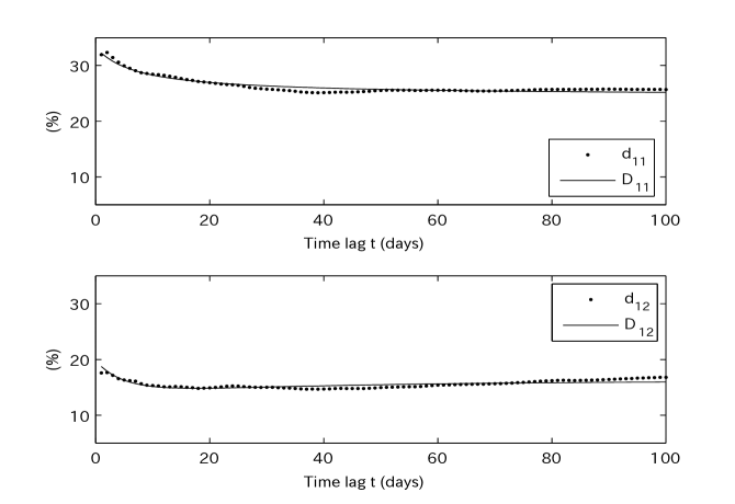
Figure C.1. $d_{11}(t)$ vs. fitted $D_{11}(t)$ and $d_{12}(t)$ vs. fitted $D_{12}(t)$.

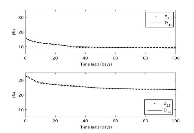
Figure C.2. $d_{13}(t)$ vs. fitted $D_{13}(t)$ and $d_{22}(t)$ vs. fitted $D_{22}(t)$.

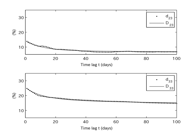
Figure C.3. $d_{23}(t)$ vs. fitted $D_{23}(t)$ and $d_{33}(t)$ vs. fitted $D_{33}(t)$.

Acknowledgements. We express our gratitude to Jun Sekine who suggested the use of a Cameron–Martin type formula in the proof of Theorem 2.3. The work of the second author was partially supported by a Research Fellowship of the Japan Society for the Promotion of Science for Young Scientists.

References

• [1] V. Anh and A. Inoue. Financial markets with memory I: Dynamic models. Stoch. Anal. Appl., 23:275–300, 2005.
• [2] V. Anh, A. Inoue and Y. Kasahara. Financial markets with memory II: Innovation processes and expected utility maximization. Stoch. Anal. Appl., 23:301–328, 2005.
• [3] V. Anh, A. Inoue and C. Pesee. Incorporation of memory into the Black–Scholes–Merton theory and estimation of volatility. Preprint.
• [4] O. E. Barndorff-Nielsen, E. Nicalato and N. Shephard. Some recent developments in stochastic volatility modelling. Quant. Finance, 2:11–23, 2002.
• [5] O. E. Barndorff-Nielsen and N. Shephard. Non-Gaussian Ornstein–Uhlenbeck-based models and some of their uses in financial economics. J. Roy. Statist. Soc. Ser. B, 63:167–241, 2001.
• [6] T. R. Bielecki and S. R. Pliska. Risk sensitive dynamic asset management. Appl. Math. Optim., 39:337–360, 1999.
• [7] F. Comte and E. Renault. Long memory continuous-time models. J. Econometrics, 73:101–149, 1996.
• [8] F. Comte and E. Renault. Long memory in continuous-time stochastic volatility models. Math. Finance, 8:291–323, 1998.
• [9] R. J. Elliott and J. van der Hoek. A general fractional white noise theory and applications to finance. Math. Finance, 13:301–330, 2003.
• [10] W. H. Fleming and R. W. Rishel. Deterministic and Stochastic Optimal Control. Springer-Verlag, New York, 1975.
• [11] W. H. Fleming and S. J. Sheu. Risk-sensitive control and an optimal investment model. Math. Finance, 10:197–213, 2000.
• [12] W. H. Fleming and S. J. Sheu. Risk-sensitive control and an optimal investment model (II). Ann. Appl. Probab., 12:730–767, 2000.
• [13] H. Hata and Y. Iida. A risk-sensitive stochastic control approach to an optimal investment problem with partial information. Preprint.
• [14] H. Hata and J. Sekine. Solving long term optimal investment problems with Cox-Ingersoll-Ross interest rates. Adv. Math. Econ., 8:231–255, 2006.
• [15] H. Hata and J. Sekine. Solving a large deviations control problem with a nonlinear factor model. Preprint.
• [16] C. C. Heyde. A risky asset model with strong dependence through fractal activity time. J. Appl. Prob., 36:1234–1239, 1999.
• [17] C. C. Heyde and N. N. Leonenko. Student processes. Adv. in Appl. Probab., 37:342–365, 2005.
• [18] Y. Hu and B. Øksendal. Fractional white noise calculus and applications to finance. Infin. Dimens. Anal. Quantum Probab. Relat. Top., 6:1–32, 2003.
• [19] Y. Hu, B. Øksendal, and A. Sulem. Optimal consumption and portfolio in a Black-Scholes market driven by fractional Brownian motion. Infin. Dimens. Anal. Quantum Probab. Relat. Top., 6:519–536, 2003.
• [20] A. Inoue, Y. Nakano and V. Anh. Linear filtering of systems with memory and application to finance. J. Appl. Math. Stoch. Anal., 2006, in press.
• [21] I. Karatzas and S. E. Shreve. Methods of mathematical finance. Springer-Verlag, New York, 1998.
• [22] K. Kuroda and H. Nagai. Risk sensitive portfolio optimization on infinite time horizon. Stoch. Stoch. Rep., 73:309–331, 2002.
• [23] R. S. Liptser and A. N. Shiryayev. Statistics of random processes. I. General theory, 2nd ed. Springer-Verlag, New York, 2001.
• [24] D. G. Luenberger, Investment science, Oxford University Press, Oxford, 1998.
• [25] R. Merton. Optimal consumption and portfolio rules in a continuous time model. J. Econom. Theory, 3:373–413, 1971.
• [26] L. E. Myers. Survival functions induced by stochastic covariance processes. J. Appl. Prob., 18:523–529, 1981.
• [27] H. Nagai and S. Peng. Risk-sensitive dynamic portfolio optimization with partial information on infinite time horizon. Ann. Appl. Probab., 12:173–195, 2002.
• [28] H. Pham. A large deviations approach to optimal long term investment. Finance Stoch., 7:169–195, 2003.
• [29] H. Pham. A risk-sensitive control dual approach to a large deviations control problem. Systems Control Lett., 49:295–309, 2003.
• [30] L. C. G. Rogers. Arbitrage with fractional Brownian motion. Math. Finance, 7:95–105, 1997.
• [31] L. C. G. Rogers and D. Williams. Diffusions, Markov processes and Martingales, Vol. 2, 2nd ed. Cambridge university press, Cambridge, 2000.
• [32] W. Willinger, M. S. Taqqu, and V. Teverovsky. Stock market prices and long-range dependence. Finance Stoch., 3:1–13, 1999.
• [33] Yahoo! Inc. Yahoo! Finance, http://finance.yahoo.com/.