Salem-Boyd sequences and Hopf plumbing

Abstract

Given a fibered link, consider the characteristic polynomial of the monodromy restricted to first homology. This generalizes the notion of the Alexander polynomial of a knot. We define a construction, called iterated plumbing, to create a sequence of fibered links from a given one. The resulting sequence of characteristic polynomials for these links has the same form as those arising in work of Salem and Boyd in their study of distributions of Salem and P-V numbers. From this we deduce information about the asymptotic behavior of the large roots of the generalized Alexander polynomials, and define a new poset structure for Salem fibered links.

1 Introduction

Let $(K,\Sigma)$ denote a fibered link $K\subset S^{3}$ with fibering surface $\Sigma$. Hopf plumbing defines a natural operation on fibered links that allows one to construct new fibered links from a given one while keeping track of useful information [Stallings:fibered] [Gabai:Murasugi]. Furthermore, a theorem of Giroux [Giroux02] shows that any fibered link can be obtained from the unknot by a sequence of Hopf plumbings and de-plumbings (see also [Harer:fibered]).

A fibered link $(K,\Sigma)$ has an associated homeomorphism $h:\Sigma\rightarrow\Sigma$, called the monodromy of $(K,\Sigma)$, such that the complement in $S^{3}$ of a regular neighborhood of $K$ is homeomorphic to a mapping torus for $h$. Let $h_{*}$ be the restriction of $h$ to first homology $\mathrm{H}_{1}(\Sigma,\mathbb{R})$, and let $\Delta_{(K,\Sigma)}(t)$ be the characteristic polynomial of the monodromy $h_{*}$. If $K$ is connected, that is, a fibered knot, then $\Delta_{(K,\Sigma)}(t)$ is the usual Alexander polynomial of $K$ and the mapping torus structure is unique. We extend this terminology and call $\Delta_{(K,\Sigma)}(t)$ the Alexander polynomial of the fibered link $(K,\Sigma)$.

A polynomial $f$ of degree $d$ is reciprocal if $f=f_{*}$, where $f_{*}(t)=t^{d}f(1/t)$. The Alexander polynomials $\Delta_{(K,\Sigma)}(t)$ are monic integer polynomials and reciprocal up to multiples of $(t-1)$. Burde [Burde:Alex] shows that there exists a fibered knot $(K,\Sigma)$ with $\Delta_{(K,\Sigma)}=f$, if and only if

(i) $f$ is a reciprocal monic integer polynomial; and

(ii) $f(1)=\pm 1$,

Kanenobu [Kanenobu81] shows that (i) is true if and only if $\Delta_{(K,\Sigma)}=f$ up to multiples of $(t-1)$, where $(K,\Sigma)$ is a fibered link. Our goal in this paper is to study how the roots of $\Delta_{(K,\Sigma)}(t)$ are affected by Hopf plumbing.

In Section 2, we define a construction called iterated (trefoil) plumbing, which produces a sequence of fibered links $(K_{n},\Sigma_{n})$ from a given fibered link $(K,\Sigma)$ and a choice of path $\tau$ properly embedded on $\Sigma$, called the plumbing locus.

Our main result is the following.

Theorem 1

If $(K_{n},\Sigma_{n})$ is obtained from $(K,\Sigma)$ by $\pm$ iterated trefoil plumbing, then there is a polynomial $P=P_{\Sigma,\tau}$ depending only on the location and orientation of the plumbing, such that $\Delta_{n}=\Delta_{(K_{n},\Sigma_{n})}$ is given by

$$\Delta_{n}(t)=\frac{t^{2n}P(t)\pm(-1)^{r}P_{*}(t)}{t+1},$$ (1)

where $r$ is the number of components of $K$.

We call sequences of polynomials of the form given in Equation 1 Salem-Boyd sequences, after work of Salem [Salem44] and Boyd [Boyd77] [Boyd89].

For a monic integer polynomial $f(t)$, let $\lambda(f)$ be the maximum absolute value among all roots of $f(t)$; $N(f)$, the number of roots with absolute value greater than one; and $M(f)$, the product of absolute values of roots of $f$ whose absolute value is greater than one. The latter invariant $M(f)$ is known as the Mahler measure of $f$. Clearly $N(f)$ is discrete, while $\lambda(f)$ can be made arbitrarily close to but greater than one, for example, by taking $f(t)=t^{n}-2$. Whether or not the values of $M(f)$ can also be brought arbitrarily close to one from above is an open problem posed by Lehmer in 1933 [Lehmer33]. Lehmer originally formulated his question as follows:

Question 2 (Lehmer)

For each $\delta>0$ does there exist a monic integer polynomial $f$ such that $1<M(f)<1+\delta$?

We are still far from answering Lehmer’s question, but show in Section 3 how to apply Salem and Boyd’s work and Theorem 1 to obtain information about the asymptotic behavior of $N(\Delta_{n})$, $\lambda(\Delta_{n})$, and $M(\Delta_{n})$ from properties of the original fibered link and location of plumbing.

Theorem 3

The sequences $N(\Delta_{n})$, $\lambda(\Delta_{n})$ and $M(\Delta_{n})$ converge to $N(P)$, $\lambda(P)$, and $M(P)$, respectively, where $P=P_{\Sigma,\tau}$.

Theorem 3 is useful for finding minimal Mahler measures appearing in particular families of fibered links, since the polynomials $P_{\Sigma,\tau}$ are easy to compute for explicit examples. We give an illustration in Section LABEL:example-section.

Iterated plumbing may be seen as the result of iterating full twists on a pair of strands of $K$, with some extra conditions on the pair of strands. For the case where $K$ has one component, the convergence of Mahler measure in Theorem 3 agrees with a result of Silver and Williams, which in general form may be stated as follows. Let $L$ be a link and $k$ an unknot disjoint from $L$ such that $L$ and $k$ have non-zero linking number. Let $L_{n}$ be obtained from $L$ by doing $1/n$ surgery along $k$. This amounts to taking the strands of $L$ encircled by $k$ and doing $n$ full-twists to obtain $L_{n}$. Silver and Williams show that the multi-variable Mahler measures of the links $L_{n}$ converge to the multi-variable Mahler measure of $L\cup k$ [S-W:Mahler]. Combining our results with that of Silver and Williams, and using the formulas for $P_{\Sigma,\tau}$ given in Section 2 (Equations 2 and 3) gives a new effective way to calculate the multi-variable Mahler measure of $L\cup k$.

It is not hard to see that if one fixes the degree of $f$, then the answer to Lehmer’s question is negative. Theorem 3 makes it possible to study Mahler measures for sequences of fibered links whose fibers have increasing genera, and hence for polynomials of increasing degree. Although, in general, $\lambda(\Delta_{n})$ and $M(\Delta_{n})$ are not monotone sequences (see Theorem 13), monotonicity can be shown (at least for large enough $n$) when $P_{\Sigma,\tau}$ has special properties.

In Section 3, we review properties of Salem-Boyd sequences, following work of Salem [Salem44] and Boyd [Boyd77], and consider the question of monotonicity. A Perron polynomial is a monic integer polynomial $f$ with a real root $\lambda=\lambda(f)>1$ satisfying $|\alpha|<\lambda$ for all roots $\alpha$ of $f$ not equal to $\lambda$.

Theorem 4

Suppose $P_{\Sigma,\tau}$ is a Perron polynomial. Then $\lambda(\Delta_{n})$ is an eventually monotone (increasing or decreasing) sequence converging to $\lambda(P_{\Sigma,\tau})$.

In the special case when $N(P_{\Sigma,\tau})=1$, more can be shown by applying results of Salem [Salem44] and Boyd [Boyd77].

Theorem 5

Suppose $N(P_{\Sigma,\tau})=1$. Then $M(\Delta_{n})=\lambda(\Delta_{n})$ is a monotone (increasing or decreasing) sequence converging to $\lambda(P_{\Sigma,\tau})$.

Section LABEL:applications-section studies the poset structure on fibered links defined by Hopf plumbing, and the corresponding poset structure on homological dilatations. We also give an example in Section LABEL:applications-section that shows how Theorem 5 can be used to give explicit solutions to Lehmer’s problem for restricted families.

Acknowledgements: I am indebted to J.S.P.S. who funded my research, and the staff of the Osaka University Mathematics Department and my host Makoto Sakuma for their kind hospitality and support during the writing of this paper. I would also like to thank D. Silver and S. Williams for many helpful discussions, and S. Williams and E. Kin for bringing my attention to the example in Section LABEL:example-section.

2 Iterations of Hopf plumbings.

We recall some basic definitions surrounding the Alexander polynomial of an oriented link. A Seifert surface for an oriented link $K$ is an oriented surface $\Sigma$ whose boundary is $K$. For any collection of free loops $\sigma_{1},\dots,\sigma_{d}$ on $\Sigma$ forming a basis for $\mathrm{H}_{1}(\Sigma;\mathbb{R})$, the associated Seifert matrix $S$ is given by

$$S=[\ell\mathrm{k}(\sigma_{i}^{+},\sigma_{j})],$$

where $\sigma_{i}^{+}$ is the push-off of $\sigma_{i}$ off $\Sigma$ into $S^{3}\setminus\Sigma$ in the positive direction with respect to the orientation of $\Sigma$, and $\ell\mathrm{k}(,)$ is the linking form on $S^{3}$. Let $S^{\mathrm{tr}}$ denote the transpose of $S$. The polynomial

$$\Delta_{K}(t)=|tS-S^{\mathrm{tr}}|$$

is uniquely defined up to units in the Laurent polynomial ring $\Lambda(t)=\mathbb{Z}[t,t^{-1}]$, and is reciprocal (it is the same if $S$ is replaced by $S^{\mathrm{tr}}$). For the purposes of this paper, we will always normalize $\Delta_{K}$ so that $\Delta_{K}(0)\neq 0$, and the highest degree coefficient of $\Delta_{K}(t)$ is positive. Then for any nonsingular Seifert matrix for $K$,

$$\Delta_{K}(t)=\mathrm{s}(S)|tS-S^{\mathrm{tr}}|,$$

where $\mathrm{s}(S)$ is the sign of the coefficient of $|tS-S^{\mathrm{tr}}|$ of highest degree.

If $K$ is fibered, and $\Sigma$ is the fibering surface, then the Seifert matrix $S$ is invertible over the integers, and the monodromy restricted to $\mathrm{H}_{1}(\Sigma;\mathbb{R})$ satisfies $h_{*}=S^{\mathrm{tr}}S^{-1}$. In this case $\mathrm{s}(S)=|S|$, and $\Delta_{K}(t)$ is characteristic polynomial of $h_{*}$. Since $|S|$ is invariant under change of basis, and the fiber surface is fixed, we will write $\mathrm{s}(K)=\mathrm{s}(S)$ if $K$ is fibered. If $K$ is a fibered knot, then $\mathrm{s}(K)=\Delta_{K}(1)$.

Figure 1: Positive Hopf plumbing

A properly embedded path on $\Sigma$ is a smooth embedding

$$\tau:[0,1]\rightarrow\Sigma$$

such that $\tau(0),\tau(1)\in\partial\Sigma$. The surface $\Sigma^{+}_{2}(\tau)$ (resp., $\Sigma^{-}_{2}$ is obtained from $\Sigma$ by positive (resp., negative) Hopf plumbing if it is obtained from $\Sigma$ by gluing on a positive (resp., negative) Hopf band as in Figure 1. The definition is independent of the orientation of $\tau$.

Set $\Sigma^{\pm}_{1}=\Sigma$. For $n\geq 1$, let $\Sigma^{\pm}_{n+1}$ be the (positive or negative) Hopf $n$-plumbing of $\Sigma$ along $\tau$, which is obtained by Hopf plumbing along $n$ paths as shown in Figure 2, starting with the vertical path $\tau$.

Figure 2: Base paths for iterated Hopf plumbings

The positive (resp., negative) Hopf $n$-plumbings can also be considered as a Murasugi sum of $\Sigma$ with the fiber surface of the torus link $T(2,n)$ (resp., $T(2,-n)$). Let $K^{\pm}_{n}(\Sigma,\tau)$ be the boundary of the surface $\Sigma^{\pm}_{n}$. For $n=1$, we have $K^{\pm}_{1}=K$. The local oriented link diagram for $K^{\pm}_{n}$ is shown in Figure 3, and $\Sigma^{\pm}_{n}$ is the corresponding Seifert surface.

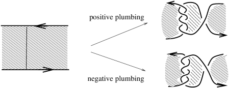
Figure 3: Result of iterated Hopf $4$-plumbing

Denote by $\langle,\rangle$ the intersection pairing

$$\mathrm{H}_{1}(\Sigma;\mathbb{Z})\times\mathrm{H}_{1}(\Sigma,\partial\Sigma;\mathbb{Z})\rightarrow\mathbb{Z},$$

and let $v\in\mathrm{H}_{1}(\Sigma;\mathbb{Z})$ be the vector such that $v^{\mathrm{tr}}$ represents the vector $[\tau]$ in $\mathrm{H}_{1}(\Sigma;\partial\Sigma;\mathbb{Q})\simeq\mathrm{H}_{1}(\Sigma;\mathbb{Q})^{\mathrm{dual}}$. Then, in terms of the basis $\sigma_{1},\dots,\sigma_{d}$, $v$ is given by

$$v=[\langle\sigma_{1},\tau\rangle,\dots,\langle\sigma_{d},\tau\rangle].$$

Set

$$P^{\pm}_{\Sigma,\tau}(t)=|tI-(S^{\mathrm{tr}}\mp vv^{\mathrm{tr}})S^{-1}|,$$ (2)

where $I$ is the identity matrix.

Before proving the Theorem 1, we put $P^{\pm}_{\Sigma,\tau}$ in an alternate form. Let $N(\tau)$ be a regular neighborhood of $\tau$ on $\Sigma$, and let $\Sigma_{0}=\Sigma\setminus N(\tau)$. Let $K_{0}=K_{0}(\Sigma,\tau)=\partial\Sigma_{0}$. Let $\sigma_{1},\dots,\sigma_{d-1}$ be a collection of free loops on $\Sigma_{0}$ forming a basis for $\mathrm{H}_{1}(\Sigma_{0};\mathbb{Z})$. Let $\sigma_{d}$ be a free loop on $\Sigma$ so that $\sigma_{1},\dots,\sigma_{d}$ is a basis for $\mathrm{H}_{1}(\Sigma;\mathbb{Z})$, and such that $\langle\sigma_{d},\tau\rangle=1$. Let $S_{1}$ and $S_{0}$ be the corresponding Seifert matrices for $K$ and $K_{0}$, respectively.

Lemma 6

The Seifert matrix $S_{0}$ is non-singular.

Proof. By our definitions, the transpose of the Seifert matrix defines a linear transformation from the first homology of the Seifert surface to its dual. We thus have a commutative diagram

$$\begin{array}[]{ccc}\mathrm{H}_{1}(\Sigma_{0};\mathbb{Z})&{\shortstack{$S_{0}^{\mathrm{tr}}$ \\ $\rightarrow$ }}&\mathrm{H}_{1}(\Sigma_{0};\mathbb{Z})^{\mathrm{dual}}\\ \vector(0,-1){12.0}&&\vector(0,-1){12.0}\\ \mathrm{H}_{1}(\Sigma_{1};\mathbb{Z})&{\shortstack{$S_{1}^{\mathrm{tr}}$ \\ $\rightarrow$}}&\mathrm{H}_{1}(\Sigma_{1};\mathbb{Z})^{\mathrm{dual}}.\end{array}$$

where vertical arrows are the inclusions determined by the choice of bases. Since $S_{1}$ is non-singular, it follows that $S_{0}$ must also be non-singular.

Lemma 7

The polynomial in Equation 2 can be rewritten as

$$P^{\pm}_{\Sigma,\tau}(t)=\Delta_{K}(t)\pm\mathrm{s}(K)\mathrm{s}(S_{0})\Delta_{K_{0}}(t).$$ (3)

Proof. The choice of basis $\sigma_{1},\dots,\sigma_{d}$ above yields the Seifert matrix S_1 = [ S_0xy^trs ] for $K$, where $x,y\in\mathbb{Z}^{d-1}$, and $s\in\mathbb{Z}$. The vector $v$ written with respect to the dual elements of $\sigma_{1},\dots,\sigma_{d}$ is given by $v=[0,\dots,0,1]^{\mathrm{tr}}$. We thus have —tS_1 - (S_1^tr∓vv^tr)— = — tS_0 - S_0^trtx - yty^tr- x^trs(t-1)±1 —. Therefore P^±_Σ,τ(t) = s(K)( —tS_1-S_1^tr— ±—tS_0 - S_0^tr—) and the claim follows.

For a polynomial $g$, define ¯g(t) = t^-mg(t), where $m$ is the largest power of $t$ dividing $g$. Then it is easy to check that $g_{*}(t)=\overline{g}_{*}(t)$. Also, if $g$ and $f$ are polynomials of degrees $d^{\prime}$ and $d$, respectively, then for $h(t)=g(t)\pm f(t)$, we have h_*(t) = g_*(t) ±t^d’-d f_*(t).

Lemma 8

Let $r$ be the number of components of $K$, and $P(t)=P^{\pm}_{\Sigma,\tau}(t)$. Then P_*(t) = (-1)^r+1(Δ_K(t) ∓s(K)s(S_0)tΔ_K_0(t)).

Proof. If $d$ is the rank of $\mathrm{H}_{1}(\Sigma;\mathbb{R})$, we have P_*(t) = t^dΔ_K(1/t) ±s(K) t^d (—(1/t)S_0-S_0^tr—). The Alexander polynomial of a link is reciprocal (anti-reciprocal) if the number of components is odd (even). Thus, the first summand equals $(-1)^{r+1}\Delta_{K}(t)$. Since, by Lemma 6, $S_{0}$ is a non-singular matrix, $t$ does not divide $|tS_{0}-S_{0}^{\mathrm{tr}}|$. It is also not difficult to check that the number of components of $K_{0}$ and $K_{1}$ have opposite parity, and the degree of $|tS_{0}-S_{0}^{\mathrm{tr}}|$ is one less than the degree of $\Delta_{K}(t)$. We thus have t^d—(1/t)S_0 - S_0^tr— = (-1)^r t —tS_0 - S_0^tr— = (-1)^r s(S_0)t Δ_K_0(t).

Theorem 1 is implied by the following stronger version.

Theorem 9

Let $(K_{n},\Sigma_{n})$ be obtained by $\pm$ iterated Hopf plumbing on a fibered link $(K,\Sigma)$ with $r$-components. Let $\Delta_{n}=\Delta_{(K_{n},\Sigma_{n})}$, and let $P=P^{\pm}_{\Sigma,\tau}$. Then Δ_n(t) = tnP(t) ±(-1)r+nP*(t)t+1.

Proof. By Lemma 8, we have

$$tP(t)+(-1)^{r+1}P_{*}(t) = t\Delta_{K}(t)\pm\mathrm{s}(K)\mathrm{s}(S_{0})t\Delta_{K_{0}}(t)$$

$$\qquad\qquad+(\Delta_{K}(t)\mp\mathrm{s}(K)\mathrm{s}(S_{0})t\Delta_{K_{0}}(t))$$

$$= (t+1)\Delta_{K}(t).$$

For $m\geq 1$, the Seifert matrix for $S^{\pm}_{m}$ is given by S^±_m=[ S^±_m-10w±1 ], where $w=[0,\dots,0,-1]$. Thus, the Alexander polynomial for $K^{\pm}_{m}$ is given by Δ_K^±_m(t) = s(K^±_m)— tS^±_m-1 - (S^±_m-1)^tr-w^trtw±(t-1) —. It follows that for $n\geq 2$, $\Delta_{K^{\pm}_{n}}(t)$ satisfies (t+1)Δ_K^±_n(t) =s(K^±_n)(t+1) [±(t-1)—tS^±_n-1-(S^±_n-1)^tr— + t—tS^±_n-2-(S^±_n-2)^tr—], and $\mathrm{s}(K^{\pm}_{n})=\pm\mathrm{s}(K^{\pm}_{n-1})$. For $n=2$, using $\mathrm{s}(K)=\mathrm{s}(K_{1})=\pm\mathrm{s}(K^{\pm}_{2})$, we have

$$(t+1)\Delta_{K^{\pm}_{2}}(t) = \mathrm{s}(K^{\pm}_{2})\left[\pm(t^{2}-1)|tS_{1}-S_{1}^{\mathrm{tr}}|+(t^{2}+t)|tS_{0}-S_{0}^{\mathrm{tr}}|\right]$$

$$= \pm\mathrm{s}(K^{\pm}_{2})((t^{2}-1)|tS_{1}-S_{1}^{\mathrm{tr}}|\pm(t^{2}+t)|tS_{0}-S_{0}^{\mathrm{tr}}|)$$

$$= \mathrm{s}(K)t^{2}(|tS_{1}-S_{1}^{\mathrm{tr}}|\pm|tS_{0}-S_{0}^{\mathrm{tr}}|)$$

$$\qquad\qquad-\mathrm{s}(K)(|tS_{1}-S_{1}^{\mathrm{tr}}|\mp t|tS_{0}-S_{0}^{\mathrm{tr}}|)$$

$$= t^{2}P(t)+(-1)^{r}P_{*}(t)$$

$$= t^{2}P(t)+(-1)^{r+2}P_{*}(t).$$

If $n>2$, we use induction, to obtain

$$(t+1)\Delta_{K^{\pm}_{n}}(t) = \pm\mathrm{s}(K^{\pm}_{n})[(t^{2}-1)|tS^{\pm}_{n-1}-(S^{\pm}_{n-1})^{\mathrm{tr}}|\pm t(t+1)|tS^{\pm}_{n-2}-(S^{\pm}_{n-2})^{\mathrm{tr}}|]$$

$$= \mathrm{s}(K^{\pm}_{n-1})[\mathrm{s}(K^{\pm}_{n-1})(t+1)(t-1)\Delta_{K^{\pm}_{n-1}}(t)$$

$$\qquad\pm\mathrm{s}(K^{\pm}_{n-2})t(t+1)\Delta_{K^{\pm}_{n-2}}(t)]$$

$$= (t-1)(t+1)\Delta_{K^{\pm}_{n-1}}(t)+t(t+1)\Delta_{K^{\pm}_{n-2}}(t)$$

$$= (t-1)(t^{n-1}P(t)+(-1)^{n-1+r}P_{*}(t))+t(t^{n-2}P(t)+(-1)^{n-2+r}P_{*}(t))$$

$$= t^{n}P(t)-t^{n-1}P(t)+(-1)^{n+r-1}tP_{*}(t)+(-1)^{n+r}P_{*}(t)$$

$$\qquad+t^{n-1}P(t)+(-1)^{n+r-2}tP_{*}(t)$$

$$= t^{n}P(t)+(-1)^{n+r}P_{*}(t)$$

3 Properties of Salem-Boyd sequences.

In this section we review some general properties of roots of polynomials in Salem-Boyd sequences (see also, [Salem44], [Boyd77]), and apply them to the Alexander polynomials of iterated plumbings.

3.1 Asymptotic behavior of roots of Salem-Boyd sequences.

Given a monic integer polynomial $P(t)$ define

$$Q^{\pm}_{n}(t) = t^{n}P(t)\pm P_{*}(t).$$ (4)

We will call the sequence of polynomials given in Equation 4 the Salem-Boyd sequence associated to $P$. For all positive integers $n$, $Q^{\pm}_{n}(t)$ is equal to a reciprocal polynomial up to a multiple of $t-1$. We are interested in the asymptotic behavior of roots of $Q^{\pm}_{n}(t)$.

S. Williams suggested the use of Rouché’s theorem to prove the following.

Lemma 10

Let $P$ be a monic integer polynomial, and let $R(t)$ be any integer polynomial, and Q_n(t) = t^n P(t) ±R(t). Then the roots of $Q_{n}(t)$ outside $C$ converge to those of $P(t)$ counting multiplicity as $n$ increases.

Proof. Consider the rational function S_n(t) = Qn(t)tn = P(t) ±R(t)tn. Let $\alpha$ be a root of $P(t)$ (counted with multiplicity), and let $D_{\alpha}$ be any small disk around $\alpha$ that is also strictly outside $C$ and that contains no roots of $P(t)$ other than $\alpha$. Then $P(t)$ has a lower bound on the boundary $\partial D_{\alpha}$, and thus there exists an $n_{\alpha}$ depending on $\alpha$ and $D_{\alpha}$ such that —R(t)tn — ¡ —P(t)— on $\partial D_{\alpha}$ for all $n>n_{\alpha}$. By Rouché’s theorem, it follows that for $n>n_{\alpha}$, $P(t)$ and $S_{n}(t)$ (and hence also $Q_{n}(t)$) have $m$ roots in $D_{\alpha}$ counted with multiplicity. Since the disks could be made arbitrarily small, and there are only a finite number of roots, the claim follows.

Lemma 11

Let $P$ be a monic integer polynomial and let $Q_{n}(t)$ be the associated Salem-Boyd sequence. Then $N(Q_{n})\leq N(P)$ for all $n$.

A proof of this Lemma is contained in [Boyd77] (p. 317), but we include it here for the convenience of the reader.

Proof. We first assume that $P(t)$ has no roots on the unit circle. This does not change the statement’s generality. To study the roots of $Q_{n}(t)$ it suffices to consider the case when $P(t)$ has no reciprocal or anti-reciprocal factors, since such factors will be factors of $Q_{n}$ for all $n$. If $P(t)$ has a root on the unit circle, then the minimal polynomial of that root would be necessarily reciprocal or anti-reciprocal, and we can factor the minimal polynomial out of $P$ and the $Q_{n}$.

Consider the two variable polynomial

$$Q_{n}(z,u)=z^{n}P(z)\pm uP_{*}(z)$$ (5)

where $z$ is any complex number and $u\in[0,1]$.

Suppose $P(t)$ has roots $\theta_{1},\dots,\theta_{s}$ outside the unit circle $C$ counted with multiplicity. Then $Q^{\pm}_{n}(z,u)$ defines an algebraic curve $z=Z(u)$ with branches $z_{1}(u),\dots,z_{s}(u)$ satisfying $z_{i}(0)=\theta_{i}$. For $z\in C$ we have $|P(z)|=|P_{*}(z)|$. Now suppose that $0<u<1$ and $1=|z_{i}(u)|$. Then 1 = —z_i(u)—^n = u—P*(zi(u))——P(zi(u))— = u yielding a contradiction. Thus, by continuity —z_i(u)— ¿ 1, for $u\in[0,1)$. It follows that $Q^{\pm}_{n}(t)$ has at most $s$ roots outside $C$.

Summarizing the contents of Lemma 10 and Lemma 11 we have the following.

Theorem 12

Let $P$ be a monic integer polynomial, and let Q_n(t) = t^n P(t) ±P_*(t). Then

$$N(Q_{n}) \leq N(P);$$

$$\lim_{n\rightarrow\infty}\lambda(Q_{n}) = \lambda(P);\quad\mbox{and}$$

$$\lim_{n\rightarrow\infty}M(Q_{n}) = M(P).$$

Theorem 1 and Theorem 12 imply Theorem 3.

A natural question is whether $M(Q_{n})$ is a monotone sequence, perhaps on arithmetic progressions, when $P$ has more than one root outside $C$. The proof of Lemma 10, does not restrict the directions by which the roots of $Q_{n}$ outside $C$ approach those of $P$. If a root $\theta$ of $P$ is not real, then the root(s) of $Q_{n}$ approaching $\theta$ typically rotate around $\theta$ as they converge. More precisely, we have the following. For $z$ a complex number, let $A=\mathrm{Arg}(z)$ be such that $z=|z|e^{2\pi iA}$.

Theorem 13

Let $\alpha_{1},\dots,\alpha_{s}$ be the roots of $P$ outside $C$. Take $N_{0}$, so that $Q_{n}$ has $s$ roots outside $C$ for $n\geq N_{0}$. Label these roots $\alpha_{i}^{(n)}$, for $i=1,\dots,s$, so that lim_n →∞ α_i^(n) = α_i. Then, there is a constant $c$ such that for any $\delta>0$, and $n>N_{\delta}>N_{0}$, Arg(α_i^(n) - α_i) = c + n Arg(α_i) + δ_n, where the error term $\delta_{n}$ satisfies $|\delta_{n}|<\delta$.

Proof. Let $P_{1}(x)$ be the largest degree monic integer factor of $P(x)$ with no roots outside $C$. For $i=1,\dots,s$, we have α_i