3-manifolds efficiently bound 4-manifolds

Abstract.

It is known since 1954 that every 3-manifold bounds a 4-manifold. Thus, for instance, every 3-manifold has a surgery diagram. There are several proofs of this fact, but there has been little attention to the complexity of the 4-manifold produced. Given a 3-manifold $M^{3}$ of complexity $n$, we construct a 4-manifold bounded by $M$ of complexity $O(n^{2})$, where the “complexity” of a piecewise-linear manifold is the minimum number of $n$-simplices in a triangulation.

The proof goes through the notion of “shadow complexity” of a 3-manifold $M$. A shadow of $M$ is a well-behaved 2-dimensional spine of a 4-manifold bounded by $M$. We further prove that, for a manifold $M$ satisfying the Geometrization Conjecture with Gromov norm $G$ and shadow complexity $S$,

$$c_{1}G\leq S\leq c_{2}G^{2}$$

for suitable constants $c_{1}$, $c_{2}$. In particular, the manifolds with shadow complexity 0 are the graph manifolds.

In addition, we give an $O(n^{4})$ bound for the complexity of a spin 4-manifold bounding a given spin 3-manifold. We also show that every stable map from a 3-manifold $M$ with Gromov norm $G$ to $\mathbb{R}^{2}$ has at least $G/10$ crossing singularities, and if $M$ is hyperbolic there is a map with at most $c_{3}G^{2}$ crossing singularities.

1. Introduction

Among the different ways to combinatorially represent 3-manifolds, two of the most popular are triangulations and surgery on a link. A triangulation is very natural way to represent 3-manifolds, and any other representation of a 3-manifold is easy to turn into a triangulation. On the other hand, although some 3-manifold invariants may be computed directly from a triangulation (e.g., the Turaev-Viro invariants), not all can be, and it is difficult to visualise the combinatorial structure of a triangulation.

A more typical way to present a 3-manifold is via Dehn surgery on a link. In practice, there are simple descriptions of small manifolds via surgery, and this is generally the preferred way of representing manifolds. There are many more invariants that may be computed directly from a surgery diagram, like the Witten-Reshetikhin-Turaev invariants. It is easy to turn a surgery diagram into a triangulation of the manifold [40]. But for the other direction, passing from triangulations to surgery diagrams, there seems to be little known. In particular, it is an open question whether a surgery diagram must (asymptotically) be more complicated than a triangulation. For a more general setting of this problem, consider that if all the surgery coefficients are integers, a surgery diagram naturally gives a 4-manifold bounded by the 3-manifold. This leads us to ask the central question of the paper:

Question 1.1.

How efficiently do 3-manifolds bound 4-manifolds?

To make this question more precise, let us make some definitions.

Definition 1.2.

A $\Delta$-complex is the quotient of a disjoint union of simplices by identifications of their faces. (See [14, Section 2.1] for a complete definition.) A $\Delta$-triangulation is a $\Delta$-complex whose underlying topological space is a manifold.

Definition 1.3.

The complexity of a piecewise-linear oriented $n$-manifold $M^{n}$ is the minimal number of $n$-simplices in a $\Delta$-triangulation of $M$.

(1) $$C(M^{n})=\min_{\text{Triang.\ $\Delta$ of $M$}}\text{\# of $n$-simplices in $\Delta$}$$

Remark 1.4.

Since the second barycentric subdivision of a $\Delta$-triangulation is an ordinary simplicial triangulation, $C(M)$ would only change by at most a constant factor if we insisted that the triangulation be simplicial.

Definition 1.5.

The 3-dimensional boundary complexity function $G_{3}(k)$ is the minimal complexity such that every 3-manifold of complexity at most $k$ is bounded by a 4-manifold of complexity at most $G_{3}(k)$.

We can think of $G_{3}(k)$ as a kind of topological isoperimetric inequality. We can now give a concrete version of our original Question 1.1:

Question 1.6.

What is the asymptotic growth rate of $G_{3}$?

The first main result of this paper is that $G_{3}(k)=O(k^{2})$. More precisely, we have

Theorem 5.2.

If a 3-manifold $M$ has a $\Delta$-triangulation with $t$ tetrahedra, then there exists a 4-manifold $W$ such that $\partial W=M$ and $W$ has a $\Delta$-triangulation with $O(t^{2})$ simplices. Moreover, $W$ has “bounded geometry”. That is, there exists an integer $c$ (not depending on $M$ and $W$) such that each vertex of the triangulation of $W$ is contained in less than $c$ simplices.

The fact that $W$ has bounded geometry makes the resulting representation nicer; in particular, to check whether the topological space resulting from a triangulation is a manifold, you need to decide whether the link of each simplex is a sphere. This is easy for dimension $n\leq 3$, in NP for $n=4$ [34], unknown for $n=5$, and undecidable for dimension $n>5$ [24, 25, 20]. In all cases, such complexity issues do not arise if the triangulation has bounded geometry.

Note that there is an evident linear lower bound for $G_{3}(k)$, since a triangulation for a 4-manifold also gives a triangulation of its boundary.

We also prove a number of other related bounds which do not directly refer to 4-manifolds. For instance, we have the following bound in terms of surgery:

Theorem 5.6.

A finite-volume hyperbolic 3-manifold with volume $V$ has a rational surgery diagram with $O(V^{2})$ crossings.

Note that there may be an infinite number of 3-manifolds with volume less than the bound $V$, and likewise an infinite number of surgeries on a given link diagram; but in both cases the manifolds come in families with some structure. In this case as well there is a linear lower bound: there are at least $V/v_{\mathrm{oct}}$ crossings in any surgery diagram for $M$, where $v_{\mathrm{oct}}\approx 3.66$ is the volume of a regular ideal hyperbolic octahedron. A somewhat weaker lower bound was proved by Lackenby [19]; the bound using $v_{\mathrm{oct}}$ comes from a decomposition into ideal octahedra, one per crossing [35, 29].

For a clean statement about general 3-manifolds, we use the crucial notion of shadows, which we recall in Section 3. For now, we just need to know that shadows are certain kinds of decorated 2-complexes which can be used to represent both a 4-manifold and a 3-manifold (on the boundary of the 4-manifold), and that a coarse notion of the complexity of a shadow is the number of its vertices. There are an infinite number of 3-manifolds with shadows with a given number of vertices, but as with hyperbolic volume and surgeries on a given link, they come in families that can be understood. The shadow complexity $\operatorname{sc}(M)$ of a 3-manifold $M$ is the minimal number of vertices in any shadow for $M$.

The following theorem says that the shadow complexity gives a coarse estimate of the hyperbolic volume.

Theorems 3.37 and 5.5.

There is a constant $C>0$ so that every geometric 3-manifold $M$, with boundary empty or a union of tori, satisfies

$$\frac{v_{\mathrm{tet}}}{2v_{\mathrm{oct}}}\|M\|\leq\operatorname{sc}(M)\leq C\|M\|^{2}.$$

The lower bound on $\operatorname{sc}(M)$ holds for all 3-manifolds.

Here $v_{\mathrm{tet}}\approx 1.01$ is the volume of a regular ideal hyperbolic tetrahedron and $v_{\mathrm{oct}}$ is as above. A geometric manifold is one that satisfies the Geometrization Conjecture [36]: it can be cut along spheres and tori into pieces admitting a geometric structure. $\|M\|$ is the Gromov norm of $M$, which is defined for any 3-manifold, and for a geometric 3-manifold is $1/v_{\mathrm{tet}}$ times the sum of the volumes of the hyperbolic pieces.

Note that there is no constant term in these theorems. The manifolds with shadows with no vertices are the graph manifolds, the geometric manifolds with no hyperbolic pieces (see Proposition 3.31).

Our techniques are based on maps from 3-manifolds to surfaces, so we can also phrase the bounds in terms of the singularities of such maps. A crossing singularity is a singularity of the type we will consider in Section 4.4: a point in $\mathbb{R}^{2}$ with two indefinite fold points in its inverse image. For more background on the classification of the stable singularities of a map from a 3-manifold to a 2-manifold, see Levine [22, 23].

Theorems 3.38 and 5.7.

A 3-manifold $M$ has at least $\|M\|/10$ crossing singularities in any smooth, stable map $\pi:M\to\mathbb{R}^{2}$. There is a universal constant $C$ so that if $M$ is hyperbolic then $M$ has a map to $\mathbb{R}^{2}$ with $C\|M\|^{2}$ crossing singularities.

One related theorem was previously known: Saeki [33] showed that the manifolds with maps to a surface with no crossing singularities are the graph manifolds.

We also prove bounds for the complexity for 3-manifolds to bound special types of 4-manifolds.

Theorem 5.3.

A 3-manifold with a triangulation with $k$ tetrahedra is the boundary of a simply-connected 4-manifold with $O(k^{2})$ 4-simplices.

Theorem 6.1.

A 3-manifold with a triangulation with $k$ tetrahedra is the boundary of a spin 4-manifold with $O(k^{4})$ 4-simplices.

All the constants in these theorems can be made explicit, but since in general they are quite bad, we have not given them explicitly. The exception is Theorems 3.37 and 3.38, which are the best possible.

As one application of the results above, let us mention computing invariants of 3-manifolds. There are a number of 3-manifold invariants that are most easily computed from a 4-manifold with boundary. (Often this is done via surgery diagrams, so the 4-manifold is simply-connected, but there are usually more general constructions as well.) For instance, the Witten-Reshitikhin-Turaev (WRT) quantum invariants are of this form [30, 39, 31] as is the Casson invariant [21].

As one concrete example, Kirby and Melvin explained [17, 18] how to compute the WRT invariant at a 4th root of unity as a sum over spin structures, which can be done concretely given a surgery diagram. Although they show that the exact evaluation is NP-hard, our results imply that the sum can be approximated (up to some error) in polynomial time using random sampling over spin structures: for any given spin structure, we can, in polynomial time, find a 4-manifold which spin-bounds the given 3-manifold and therefore compute the summand at this spin structure. This contrasts with a result of Kitaev and Bravyi, who showed that computing (up to the same error) the partition function of the corresponding 2-dimensional TQFT is BQP-complete, as soon as we allow evaluation of observables on closed curves [1].

Acknowledgments We would like to warmly thank Riccardo Benedetti, Simon King, Robion Kirby, William Thurston, Vladimir Turaev, and an anonymous referee for their encouraging comments and suggestions.

1.1. Plan of the paper

In the remainder of the Introduction, we survey some related work, first on different kinds of topological isoperimetric functions, and second on other work considering our main tool, stable maps from a 3-manifold to $\mathbb{R}^{2}$. In Section 2, we sketch our construction in the smooth setting and introduce the crucial tool of the Stein factorization, which shows how 2-complexes naturally arise. This section is not logically necessary for the rest of the paper, although it does provide helpful motivation and a guide to the proof. This 2-complexes that arise are studied more abstractly in Section 3, where we review the definition of shadow surface and prove a number of properties of them; here we also use the Gromov norm to prove all the lower bounds in the theorems above. In Section 4 we give our main tool, a construction of a shadow from a triangulated 3-manifold with a map to the plane, together with a bound on the complexity of the resulting shadow. Section 4 is independent from Section 3 except for the definition of shadows, and only uses Section 2 as motivation, so the impatient reader can skip there. In Section 5 we use this construction to prove the upper bounds of our main theorems (except for the spin bound case, Theorem 6.1) and see precisely how shadow complexity relates to geometric notions on the complexity of the manifold. Finally, in Section 6 we show how to modify an arbitrary shadow to get a 4-manifold that spin-bounds a specified spin structure on a 3-manifold, while controlling the complexity.

1.2. Related questions

Although the question we consider does not seem to have been previously addressed, there has been related work. Perhaps the closest is the work on distance in the pants complex and hyperbolic volumes. The pants complex is closely related to shadows; in particular, a sequence of moves of length $n$ in the pants complex can be turned into a shadow with $n$ vertices for a 3-manifold which has two boundary components, so that the natural pants decomposition of the boundary components corresponds to the start and end of the sequence of moves.

Theorem 1.7 (Brock [2, 3]).

Given a surface $S$ of genus $g\geq 2$, there are constants $C_{1},C_{2}$ so that for every pseudo-Anosov map $\psi:S\to S$, we have

$$C_{1}\|\psi\|_{\mathrm{P}ants}\leq\operatorname{vol}(T_{\psi})\leq C_{2}\|\psi\|_{\mathrm{P}ants}$$

where $T_{\psi}$ is the mapping torus of $\psi$ and $\|\psi\|_{\mathrm{P}ants}$ is the translation distance in the pants complex.

By the relation between moves in the pants complex and shadows mentioned above, this shows that for 3-manifolds that fiber over the circle with fiber a surface of fixed genus, shadow complexity is bounded above and below by a linear function of the hyperbolic volume. However, the constant depends on the genus in an uncontrolled way. Our result gives a quadratic bound, but with an explicit constant not depending on the genus. Brock’s construction also produces shadows (and 4-manifolds) of a particular type.

More recently, Brock and Souto have announced [4] that there is a similar bound for manifolds with a Heegaard splitting with a fixed genus. In our language, their result says that a hyperbolic manifold with a strongly irreducible Heegaard splitting of genus $g$ has a shadow diagram where the number of vertices is bounded by a linear function of the volume, with a constant of proportionality depending only on the genus. (The result is probably true without the assumption that the Heegaard splitting is strongly irreducible, but the statement becomes more delicate in the language of the pants complex and we have not checked the details.) Their method of proof does not produce any explicit constants.

There has also been work on the question of polygonal curves in $\mathbb{R}^{3}$ bounding surfaces.

Definition 1.8.

The surface isoperimetric function $G_{\text{\rm{surf}}}(k)$ is the minimal number such that every closed polygonal curve $\gamma$ in $\mathbb{R}^{3}$ with at most $k$ segments bounds an oriented polygonal surface $\Sigma$ with at most $G_{\text{\rm{surf}}}(k)$ triangles.

Theorem 1.9 (Hass-Lagarias [9]).

$\frac{1}{2}k^{2}\leq G_{\text{\rm surf}}(k)\leq 7k^{2}.$

This result contrasts sharply with the situation when we ask for the spanning surface $\Sigma$ to be a disk.

Definition 1.10.

The disk isoperimetric function $G_{\text{{disk}}}(k)$ is the minimal number such that every closed polygonal curve $\gamma$ in $\mathbb{R}^{3}$ with at most $k$ segments bounds an oriented polygonal disk $D$ with at most $G_{\text{{surf}}}(k)$ triangles.

Theorem 1.11 (Hass-Snoeyink-Thurston [11]).

$G_{\text{\rm{disk}}}(k)=e^{\Omega(k)}$. That is, there is a constant $C$ so that, for sufficiently large $k$, $G_{\text{\rm{disk}}}(k)\geq e^{Ck}$.

Theorem 1.12 (Hass-Lagarias-Thurston [10]).

$G_{\text{{disk}}}(k)=e^{O(k^{2})}$. That is, there is a constant $C$ so that, for sufficiently large $k$, $G_{\text{\rm{disk}}}(k)\leq e^{Ck^{2}}$.

Although there is a large gap between these upper and lower bounds, both bounds are substantially larger than the bounds in Theorem 1.9, which was about arbitrary oriented surfaces.

There is an analogous question on the growth of $G_{\text{\rm{disk}}}$ for 3-manifolds rather than curves: asking for 4-balls bounding a 3-sphere with a given triangulation on the boundary. As stated, this is not an interesting question, since we can construct such a triangulation by taking the triangulated 3-ball and coning it to a point. This is related to the somewhat unsatisfactory nature of the 4-manifold complexity (mentioned earlier). A more interesting question might involve 4-manifold triangulations where the vertices have bounded geometry. For a somewhat different question, there are known upper bounds:

Definition 1.13.

The Pachner isoperimetric function $G_{\text{{Pachner}}}(k)$ is the maximum over all triangulations $T$ of the 3-sphere with $\leq\,k$ simplices of the minimum number of Pachner moves required to relate $T$ to the standard triangulation, the boundary of a 4-simplex.

Theorem 1.14 (King [16], Mijatović [28]).

$G_{\text{\rm{Pachner}}}(k)=e^{O(k^{2})}$.

Note that a sequence of Pachner moves as in the definition gives you, in particular, a triangulation of the 4-ball, although you only get very special triangulations of the 4-ball in this way.

As in the case of polygonal surfaces and disks, this upper bound is much larger than the polynomial bound we obtain. King [16] also constructs triangulations of $S^{3}$ which seem likely to require a large number of Pachner moves to simplify.

1.3. Previous work

The central construction in our proof, a generic smooth map from a 3-manifold to $\mathbb{R}^{2}$, has been considered by several previous authors, sometimes with little contact with each other. These maps were probably first considered by Burlet and de Rham [5], who showed that the 3-manifolds admitting a map with only definite fold singularities are connected sums of $S^{1}\times S^{2}$ (including $S^{3}$). They also introduced the Stein factorization. Levine [23] clarified the structure of the singularities and studied, for instance, related immersions of the 3-manifold into $\mathbb{R}^{4}$. Burlet and de Rham’s result was extended by Saeki [33], who showed that the 3-manifolds admitting a map without codimension 2 singularities (i.e., only definite or indefinite folds) are the graph manifolds.

Rubinstein and Scharlemann [32] constructed a map from the complement of a graph in a 3-manifold to $\mathbb{R}^{2}$ from a pair of Heegaard splittings and used this to bound the number of stabilizations required to turn one splitting into the other. Much of the analysis is similar to ours.

Also independently, Hatcher and Thurston [12] considered Morse functions on a orientable surface to show that its mapping class group is finitely presented. To get a set of generators, they considered one parameter deformations of the Morse function. Note that a one parameter family of maps from $\Sigma$ to $\mathbb{R}$ is a map from the 3-manifold $\Sigma\times[0,1]$ to $\mathbb{R}^{2}$.

In a slightly different context, Hatcher’s proof of the Smale conjecture [13], that the space of smooth 2-spheres in $\mathbb{R}^{3}$ is contractible, uses the Stein factorization of a map from $S^{2}$ to $\mathbb{R}^{2}$. Hong, McCullough, and Rubinstein recently combined this approach with the Rubinstein-Scharlemann techniques in their proof of the Smale conjecture for lens spaces [15].

On the other side of the story, Turaev [37, 38, 39] introduced shadow surfaces as the most natural objects on which the Reshetikhin-Turaev quantum invariants are defined. He observed that you could construct both a 3-manifold and a 4-manifold with boundary the 3-manifold from a shadow surface.

Thus several authors have been considering nearly the same objects (shadow surfaces on the one hand and the Stein factorization of a map from $M^{3}$ to $\mathbb{R}^{2}$ on the other hand) for several years. The gleams are key topological data from the shadow surface point of view, since they let you reconstruct the 3-manifold, but they were not explicitly described by the authors writing on Stein factorizations, although it is implicitly present.

2. 4-manifolds from stable maps

In order to prove that 3-manifolds efficiently bound 4-manifolds, we start by sketching a proof that 3-manifolds do bound 4-manifolds. In Section 4 we will analyze a version of the proof in the PL setting and give a bound on the complexity of the resulting 4-manifold.

Consider an oriented, smooth, closed 3-manifold $M^{3}$ and a generic smooth map $f$ from $M$ to $\mathbb{R}^{2}$. At a regular value $x\in\mathbb{R}^{2}$, the inverse image $f^{-1}(x)$ consists of an oriented union of circles. To construct a 4-manifold, we glue a disk to each of these circles away from critical values and then extend across the singularities in codimension 1 and codimension 2.

2.1. Pants decompositions from Morse functions

To get some idea of what the singularities look like, we first do the analysis of extending across singularities one dimension down: let’s prove that every oriented 2-manifold $\Sigma^{2}$ bounds a 3-manifold. Consider a generic smooth map $f$ from $\Sigma$ to $\mathbb{R}$, that is, a Morse function. The inverse image of a regular value is again a union of circles. Glue in disks to each of these circles as in Figure 1. More properly, take $\Sigma\times[0,1]$, pick a regular value in each component of $\mathbb{R}$ minus the singular set, and attach 2-handles along the circles appearing in the inverse image of the chosen regular values. The result is a 3-manifold with one boundary component which is $\Sigma$ and other boundary components corresponding to the singular values of $f$.

$$\vbox{\hbox{\includegraphics[trim=-1.00374pt -1.00374pt -1.00374pt -1.00374pt]{draws/surface.62}}}\longrightarrow\vbox{\hbox{\includegraphics[trim=-1.00374pt -1.00374pt -1.00374pt -1.00374pt]{draws/surface.71}}}$$

Figure 1. Proving that every surface bounds a 3-manifold: A generic map of a surface to $\mathbb{R}$, with regular values marked and disks glued into the inverse image of the regular values.

The singular values of a Morse function, locally in the domain $\Sigma$, are well-known: they are critical points with a quadratic form which is definite (index 0 or 2, minima or maxima) or indefinite (index 1, saddle points). Since our construction works with the entire inverse image of a regular value, we need to understand the singularities locally in the range $\mathbb{R}$; that is, we need to know the connected components of inverse images of a critical value. This is easy for the definite singularities.

Let $p_{0}\in\Sigma$ be a saddle point, and let $x_{0}\in\mathbb{R}$ be its image. Near $p_{0}$, $f^{-1}(x_{0})$ is a cross. For $x$ above and below $x_{0}$, $f^{-1}(x)$ is locally the cross is smoothed out in the two possible ways. Note that the orientations of $\Sigma$ and $\mathbb{R}$ induce an orientation of $f^{-1}(x)$ for all $x\in\mathbb{R}$ except at critical points in $\Sigma$, so both of these smoothings must be oriented, so the arms of the cross must be oriented alternating in and out. The connected component of $f^{-1}(x_{0})$ containing $p_{0}$ must join the arms of the cross in an orientation-preserving way and is therefore a figure 8 graph  . This implies that for a small interval $I$ containing $x_{0}$, $f^{-1}(I)$ is a pair of pants.

             

Figure 2. Analysing the saddle singularity

To finish constructing the 3-manifold, recall that in the previous step we glued in disks at all the regular values. Near this pair of pants, this means that we have closed off each hole in the pair of pants and the boundary component we are trying to fill in is just a sphere, which we can fill in with a ball.

An easier analysis shows that the surface we need to fill in the other cases of a maximum or minimum is again a sphere.

Notice where the proof breaks down if we do not assume that $\Sigma$ is oriented: there is then another possibility for the inverse image of the critical value, with opposite arms of the cross attached to each other: . In this case the surface we are left to fill in turns out to be $\mathbb{RP}^{2}$, which does not bound a 3-manifold.

In a similar way we can analyse the possible stable singularities of a smooth map from a 3-manifold $M$ to $\mathbb{R}^{2}$. We glue in a disk (a 2-handle) to each circle in the inverse image of a regular point, extend across codimension 1 singularities by attaching 3-handles (the singularities look just like the singularities we analysed for the case of a surface, crossed with $\mathbb{R}$), and then consider the codimension 2 singularities. In Section 4.4, we will analyze the codimension 2 singularities (in the PL category) and see that the remaining boundary from each codimension 2 singularity is $S^{3}$, which can be filled in by attaching a 4-handle.

2.2. Stein factorization and shadow surfaces

For a more global view, we can consider the Stein factorization $f=g\circ h$ of these maps. The Stein factorization of a map $f$ with compact fibers decomposes it as the composition of a map $h$ with connected fibers and a map $g$ which is finite-to-one. That is, $h$ is the quotient onto the space of connected components of the fibers of $f$. See Figure 3 for an example.

$$\vbox{\hbox{\includegraphics[trim=-1.00374pt -1.00374pt -1.00374pt -1.00374pt]{draws/surface.63}}}\overset{h}{\longrightarrow}\vbox{\hbox{\includegraphics[trim=-1.00374pt -1.00374pt -1.00374pt -1.00374pt]{draws/surface.75}}}\overset{g}{\longrightarrow}\vbox{\hbox{\includegraphics[trim=-1.00374pt -1.00374pt -1.00374pt -1.00374pt]{draws/surface.72}}}$$

Figure 3. The Stein factorization $f=g\circ h$ of the map in Figure 1.

For a stable map from an oriented surface $\Sigma$ to $\mathbb{R}$, the Stein factorization is generically a 1-manifold, with singularities from the critical points. Concretely, it is a graph with vertices which have valence 1 (at definite singularities) or valence 3 (at indefinite singularities). The surface is a circle bundle over this Stein graph $\Gamma$ at generic points. Likewise, the 3-manifold we constructed (with boundary $\Sigma$) is a disk bundle over $\Gamma$ at generic points. In fact, the 3-manifold collapses onto $\Gamma$. If we collapse all the valence 1 ends, we may think of $\Gamma$ as representing a pair-of-pants decomposition of $\Sigma$; each circle in the pair-of-pants decomposition bounds a disk in the 3-manifold.

For a stable map from a 3-manifold to $\mathbb{R}^{2}$, on the other hand, the Stein factorization is generically a surface. The codimension 1 singularities of the Stein surface are products of the lower-dimensional singularities with an interval, and have one or three sheets meeting at an edge at what we will call definite or indefinite folds, respectively. In codimension two there are a few different configurations of how the surface can meet, the most interesting of which is shown in Figure 4.

             

Figure 4. Some local models for the Stein factorization of a map from a 3-manifold to $\mathbb{R}^{2}$ in codimension 0, 1, and 2. In each picture, the map to the plane is the vertical projection.

The 3-manifold is a circle bundle over the Stein surface at generic points and the 4-manifold is generically a disk bundle. As in the previous case, it turns out that the 4-manifold collapses onto the Stein surface. The resulting surface is very close to a shadow surface.

Unlike in the lower dimensional case, the surface does not determine the 4-manifold (or the 3-manifold), even after you fix a standard local model of how the surface sits inside the 4-manifold. The additional data you need are the gleams, numbers associated to the 2-dimensional regions of the surface; see Definition 3.7.

3. Shadow surfaces

We will now define shadow surfaces and shadows of 3-manifolds and give a few examples. In the Section 3.2 we will extend the definitions to 3-manifolds with boundary and an embedded, framed graph. For a more detailed though introductory account of shadows of 3- and 4-manifolds, see [7]. Note that these are slightly different from the Stein surfaces mentioned in Section 2.2. We prefer shadow surfaces as the fundamental object since they are a little more symmetric and regular than Stein surfaces. From now on every manifold will be PL compact and oriented unless explicitly stated and every polyhedron will be finite; we also recall that, in dimension 3 and 4, each PL manifold has a unique smooth structure and vice versa.

3.1. Shadows of 3-manifolds

For simplicity, we will first define shadows in the case when there is no boundary, appropriate for 3-manifolds without boundary or other decorations; in the next section we will extend this.

Definition 3.1.

A simple polyhedron $P$ is a compact topological space where every point has a neighborhood homeomorphic to an open set in one of the local models depicted in Figure 5. The set of points without a local model of the leftmost type form a 4-valent graph, called the singular set of the polyhedron and denoted $\operatorname{Sing}(P)$. The vertices of $\operatorname{Sing}(P)$ are called vertices of $P$. The connected components of $P\setminus\operatorname{Sing}(P)$ are called the regions of $P$. The set of points of $P$ whose local models correspond to the boundaries of the blocks shown in the figure is called the boundary of $P$ and is denoted $\partial P$; $P$ is said to be closed if it has empty boundary. A region is internal if its closure does not touch $\partial P$. A simple polyhedron is standard if every region of $P$ is a disk, and hence $\operatorname{Sing}(P)$ has no circle components.

Definition 3.2.

Let $W$ be a PL, compact and oriented 4-manifold. $P\subset W$ is a shadow for $W$ if $P$ is a closed simple sub-polyhedron onto which $W$ collapses and $P$ is locally flat in $W$, that is for each point $p\in P$ there exists a local chart $(U,\phi)$ of $W$ around $p$ such that $\phi(P\cap U)$ is contained in $\mathbb{R}^{3}\subset\mathbb{R}^{4}$.

It follows from this definition that in the 3-dimensional slice, the pair $(\mathbb{R}^{3}\cap\phi(U),\allowbreak\mathbb{R}^{3}\cap\phi(U\cap P))$ is PL-homeomorphic to one of the models depicted in Figure 5.

For the sake of simplicity, from now on we will skip the PL prefix and all the homeomorphisms will be PL unless explicitly stated. Not every 4-manifold admits a shadow: a necessary and sufficient condition for $W$ to admit one is that it has an handle decomposition containing no handles of index greater than 2 [37, 6]. This imposes restrictions on the topology of $W$. For instance, its boundary has to be a non-empty connected 3-manifold.

$$\begin{array}[]{c@{\qquad\qquad}c@{\qquad\qquad}c}\vbox{\hbox{\includegraphics[trim=-1.00374pt -1.00374pt -1.00374pt -1.00374pt]{draws/surface.110}}}&\vbox{\hbox{\includegraphics[trim=-1.00374pt -1.00374pt -1.00374pt -1.00374pt]{draws/surface.111}}}&\vbox{\hbox{\includegraphics[trim=-1.00374pt -1.00374pt -1.00374pt -1.00374pt]{draws/surface.112}}}\\ \textrm{Region}&\textrm{Edge}&\textrm{Vertex}\end{array}$$

Figure 5. For each point of a simple polyhedron embedded in a 4-manifold there is a local chart $(U,\phi)$ in which the polyhedron is flat in the sense that is embedded in a three dimensional plane and in this plane it appears as in one of the three models shown in this figure.

Definition 3.3.

A shadow of an oriented, closed 3-manifold $M$ is a shadow $P$ of a closed 4-manifold $W$ with $M=\partial W$.

Theorem 3.4 (Turaev [37]).

Any closed, oriented, connected 3-manifold has a shadow.

Example 3.5.

The simple polyhedron $P=S^{2}$ is a shadow of $S^{2}\times D^{2}$ and hence of the 3-manifold $S^{2}\times S^{1}$. In this case, $P$ is a surface whose self-intersection number in the ambient 4-manifold is zero. Consider now the disk bundle over $S^{2}$ with Euler number equal to 1, homeomorphic to a punctured $\mathbb{CP}^{2}$. The 0-section of the bundle is a shadow of the 4-manifold homeomorphic to $P$ and so $P$ is a shadow of $\mathbb{CP}^{2}-B^{4}$ and of its boundary: $S^{3}$.

The above example shows that the naked polyhedron by itself is not sufficient to encode the topology of the 4-manifold collapsing on it. Turaev described [37] how to equip a polyhedron embedded in a 4-manifold with combinatorial data called gleams which are sufficient to encode the topology of the regular neighborhood of the polyhedron in the manifold. A gleam is a coloring of the regions of the polyhedron with values in $\frac{1}{2}\mathbb{Z}$, with value modulo 1 given by a $\mathbb{Z}_{2}$-gleam which depends only on the polyhedron.

In the simplest case, if $P$ is a shadow of $M$ and $P$ is homeomorphic to an orientable surface, then $W$ is homeomorphic to an oriented disk bundle over the surface and the gleam of $P$ is the Euler number of the normal bundle of $P$ in $W$.

We summarize in the following proposition the basic construction of the $\mathbb{Z}_{2}$-gleam and of the gleam of a simple polyhedron. A framing for a graph $G$ in a 3-manifold $M$ is a surface with boundary embedded in $M$ and collapsing onto $G$.

Proposition 3.6.

Let $P$ be a simple polyhedron. There exists a canonical $\mathbb{Z}_{2}$-coloring of the internal regions of $P$ called the $\mathbb{Z}_{2}$-gleam of $P$. If $P$ is embedded in a 4-manifold $W$ in a flat way, there is a canonical coloring of the internal regions of $P$ by integers or half-integers called gleams, such that the gleam of a region of $P$ is an integer if and only if its $\mathbb{Z}_{2}$-gleam is zero. Moreover, if $\partial P\subset\partial W$ is framed, then the gleam can also be defined on the non-internal regions of $P$.

Proof..

Let $D$ be an internal region of $P$ and let $\overline{D}$ be the abstract compactification of the (open) surface represented by $D$. The embedding of $D$ in $P$ extends to a map $i:\overline{D}\to P$ which is injective on $\operatorname{int}(\overline{D})$, locally injective on $\partial\overline{D}$ and sends $\partial\overline{D}$ into $\operatorname{Sing}(P)$. Using $i$ we can “pull back” a small open regular neighborhood of $D$ in $P$ and construct a simple polyhedron $U(D)$ collapsing on $\overline{D}$. Extend $i$ as a local homeomorphism $i^{\prime}:U(D)\to P$ whose image is contained in a small regular neighborhood of the closure of $D$ in $P$. In the particular case when $i$ is an embedding of $\overline{D}$ in $P$, $U(D)$ is the regular neighborhood of $D$ in $P$ and $i^{\prime}$ is its embedding in $P$. In general, $U(D)$ has the following structure: each boundary component of $\overline{D}$ is glued to the core of a band (annulus or Möbius strip) and some small disks are glued along half of their boundary on segments which are properly embedded in these bands and cut transversally once their cores. We define the $\mathbb{Z}_{2}$-gleam of $D$ in $P$ to be equal to the reduction modulo 2 of the number of Möbius strips used to construct $U(D)$. This coloring only depends on the combinatorial structure of $P$.

Let us now suppose that $P$ is embedded in a 4-manifold $W$, and let $D$, $\overline{D}$, $i:\overline{D}\to P$, $U(D)$ and $i^{\prime}$ be defined as above. Using $i^{\prime}$, we can “pull back” a neighborhood of $\overline{D}$ in $W$ to an oriented 4-ball $B^{4}$ collapsing on $U(D)$. The regular neighborhood of a point $p_{0}\in\partial\overline{D}\subset U(D)$ sits in a 3-dimensional slice $B^{3}_{0}$ of $B^{4}$ where it appears as in Figure 6. The direction along which the other regions touching $\partial\overline{D}$ get separated gives a section of the bundle of orthogonal directions to $D$ in $B^{4}$. (If $p_{0}\in\partial P$, use the framing of $\partial P$ in place of the other regions. By an orthogonal direction we mean a line in the normal bundle, not a ray.) This section can be defined on all $\partial\overline{D}$ and the obstruction to extend it to all of $\overline{D}$ is an element of $H^{2}(\overline{D},\partial\overline{D};\pi_{1}(S^{1}))$. Since $B^{4}$ is oriented, we can canonically identify this element with an integer and define the gleam of $D$ to be half this number.

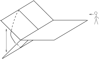
Figure 6. The picture sketches the position of the polyhedron in a 3-dimensional slice of the ambient 4-manifold. The horizontal plane is our region of interest $D$. The direction indicated by the vertical double arrow is the one along which the two regions touching the horizontal one get separated.

∎

We can also go the other direction, from gleams to 4-manifolds.

Definition 3.7.

A gleam on a simple polyhedron $P$ is a coloring on all the regions of $P$ with values in $\frac{1}{2}\mathbb{Z}$ such that the color of each internal region is integer if and only if its $\mathbb{Z}_{2}$-gleam is zero.

Theorem 3.8 (Reconstruction of 4-manifold [37]).

Let $P$ be a polyhedron with gleams $g$; there exists a canonical reconstruction associating to $P$ and $g$ a pair $(W_{P},P)$ where $W_{P}$ is a PL, compact and oriented 4-manifold containing a properly embedded copy of $P$ with framed boundary, onto which it collapses and such that the gleam of $P$ in $W_{P}$ coincides with $g$. The pair $(W_{P},P)$ can be explicitly reconstructed from the combinatorics of $P$ and from its gleam. Moreover, if $P$ is a polyhedron embedded in a PL and oriented manifold $W$, $\partial P$ is framed, and $g$ is the gleam induced on $P$ as explained in the Proposition 3.6, then $W_{P}$ is homeomorphic to the regular neighborhood of $P$ in $W$.

Hence, to study 4-manifolds with shadows (and their boundaries), one can either use abstract polyhedra equipped with gleams or embedded polyhedra.

From now on, each time we speak of a shadow of a 3-manifold as a polyhedron we will be implicitly taking a 4-dimensional thickening of this polyhedron whose boundary is the given 3-manifold or, equivalently, a choice of gleams on the regions of the polyhedron.

Example 3.9.

Let $M$ be a 3-manifold which collapses onto a simple polyhedron $P$ whose regions are orientable surfaces; it is straightforward to check that the $\mathbb{Z}_{2}$-gleam of $P$ is everywhere zero. Let us then equip $P$ with the gleam which is zero on all the regions; Turaev’s thickening construction produces the 4-manifold $W=M\times[-1,1]$ and $P$ is a shadow of $\partial W$, homeomorphic to the double of $M$.

3.2. Shadows of framed graphs in manifolds with boundary

In this subsection we extend the definition of shadows to pairs $(M,G)$ where $M$ is a 3-manifold, possibly with boundary and $G\subset M$ is a (possibly empty) framed graph with trivalent vertices and univalent ends. To do this, we allow the simple polyhedron to have boundary.

Definition 3.10.

A boundary-decorated simple polyhedron $P$ is a simple polyhedron where $\partial P$ is equipped with a cellularization whose 1-cells are colored with one of the following colors: $i$ (internal), $e$ (external) and $f$ (false). We can correspondingly distinguish three subgraphs of $\partial P$ intersecting only in $0$-cells and whose union is $\partial P$: let us call them $\partial_{i}P$, $\partial_{e}P$, and $\partial_{f}P$. A boundary-decorated simple polyhedron is said to be proper if $\partial_{f}(P)=\emptyset$.

We can turn decorated polyhedra into shadows. The intuition is that $\partial_{f}(P)$ is ignored, $\partial_{e}(P)$ is drilled out to create the boundary of the 3-manifold, and $\partial_{i}(P)$ gives a trivalent graph.

Definition 3.11.

Let $P$ be a boundary-decorated simple polyhedron, properly embedded in a 4-manifold $W$ which collapses onto $P$ with a framing on $\partial_{i}(P)$. Let $M$ be the complement of an open regular neighborhood of $\partial_{e}P$ in $\partial W$, and let $G$ be a framed graph whose core is $\partial_{i}(P)$. Then we say that $P$ is a shadow of $(M,G)$ and, if $\partial_{f}P=\emptyset$, we call it a proper shadow. As before, we can define a gleam on each region of $P$ that does not meet $\partial_{f}(P)\cup\partial_{e}(P)$.

Remark 3.12.

Turaev’s Reconstruction Theorem extends to the case of decorated polyhedra equipped with gleams on the regions not touching $\partial_{e}P\cup\partial_{f}P$.

Remark 3.13.

The genus of a boundary component of $M$ equals the rank of $H_{1}$ of the corresponding component of $\partial_{e}(P)$, since the Euler characteristic of the handlebody filling the boundary component equals the Euler characteristic of the graph. In particular, components of $\partial_{e}(P)$ corresponding to sphere boundary components of $M$ are contractible and so if $\partial_{f}(P)$ is empty, $M$ does not have any sphere boundary components that do not meet $G$.

Theorem 3.14 (Turaev [37]).

Let $M$ be a oriented, connected 3-manifold and let $G$ be a properly-embedded framed graph in $M$ with vertices of valence 1 or 3. If $M$ has no spherical boundary components that do not meet $G$, the pair $(M,G)$ has a proper, simply-connected shadow.

Let us now show how to construct a shadow of a pair $(M,G)$ given a shadow $P$ of $(M,\emptyset)$. Recall that $M$ is the boundary of a 4-manifold collapsing through a projection $\pi$ onto $P$. Up to small isotopies, we can suppose that the restriction to $G$ of $\pi$ is transverse to $\operatorname{Sing}(P)$ and to itself; that is, it does not contain triple points or self tangencies and is injective on the vertices of $T$. Let us also suppose that it misses $\partial_{f}(P)$. Then the mapping cylinder of the projection of $G$ in $P$ is contained in the thickening $W_{P}$ of $P$ and $W_{P}$ collapses on it. (Recall that the mapping cylinder is $P\cup G\times[0,1]$, with $G\times\{0\}$ identified with $\pi(G)\subset P$.) By Proposition 3.6 we can equip this polyhedron with gleams. Coloring $G\times\{1\}$ with the color $i$ we get a shadow of the pair $(M,G)$, coloring it with $e$ we get a shadow of $M-U(G)$ where $U(G)$ is a small open regular neighborhood of $G$ in $M$, and coloring it with $f$ we get another shadow of $M$ (necessarily not proper).

As a warm up, note that a flat disk $D$ whose boundary has color $f$ is a shadow of the pair $(S^{3},\emptyset)$. The open solid torus $T_{h}=\pi^{-1}(\operatorname{int}(D))$ can be imagined as the regular neighborhood of the closure of the $z$-axis in $\mathbb{R}^{3}$, embedded inside $S^{3}$ in the standard way. The fibers of $\pi:S^{3}\to D$ run parallel to the $z$-axis away from $\infty$ and are unknotted. The projection of the solid torus $T_{v}=S^{3}\setminus T_{h}$ is $\partial D$.

With the setup above, we now apply the projection construction to the case of a link $L$ in $S^{3}$. Up to isotopy we can suppose that $L\subset T_{h}$ and that its projection to $D$ is generic; so it is sufficient to consider a standard diagram of $L$ in the unit disk in $\mathbb{R}^{2}$. The mapping cylinder $D_{L}$ of $\pi:L\to D$ is obtained from $D$ by gluing an annulus for each component of $L$ and marking the free boundary components of these annuli with the color $i$. We can further collapse the region of $D_{L}$ containing $\partial_{f}D$; this produces a simple sub-polyhedron of $D_{L}$, which we call $P_{L}$. By construction $\partial P_{L}=\partial_{i}P_{L}=L$.

In general, $P_{L}$ has some vertices, each corresponding to a crossing in the diagram of $L$. However, some of the crossings in that diagram of $L$ do not generate vertices in $P_{L}$ because they disappear when we pass from $D_{L}$ to $P_{L}$.

Example 3.15.

Applying the construction to a figure eight knot in a standard position, one gets a shadow of its complement containing only one vertex: Three of the four crossings of the diagram are contained in the boundary of the region to be collapsed in $P_{L}$. See Figure 7.

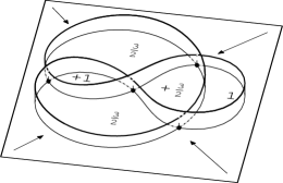
$$\to\vbox{\hbox{\includegraphics[trim=-1.00374pt -1.00374pt -1.00374pt -1.00374pt]{draws/shadow.2}}}$$

$$=\vbox{\hbox{\includegraphics[trim=-1.00374pt -1.00374pt -1.00374pt -1.00374pt]{draws/shadow.11}}}$$

Figure 7. In the left part of the picture we sketch the construction described in Example 3.15; the resulting shadow is drawn in the right part where, for the two internal regions we write their gleams. Note that, after the collapse of the polyhedron $D_{L}$ along its free boundary component (as indicated by the arrows), the only vertex surviving is the central one.

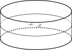
Figure 8. The shadow obtained for the Hopf link.

Example 3.16.

Consider a standard Hopf link in $T_{h}$. The polyhedron $H$ one gets by applying the above procedure contains no vertices: the two crossings of the standard projection of the Hopf link in $\mathbb{R}^{2}$ touch the region of $D$ which is collapsed. The resulting polyhedron can be obtained by gluing a disk to the core of an annulus; its embedding in $B^{4}$ is such that $\partial H$ is the Hopf link in $\partial B^{4}$. See Figure 8.

Example 3.17.

Applying this construction to the graph $\partial P$ in Figure 19 (with the projection shown there) gives the shadow in Figure 20.

3.3. Shadow complexity and its basic properties

We will now define a notion of shadow complexity and study how it behaves under combining manifolds, either via connect sum (gluing along spheres) or torus connect sum (gluing along torus boundaries).

Definition 3.18.

For $M$ be an oriented 3-manifold (possibly with boundary) and $T\subset M$ a trivalent graph, the shadow complexity $\operatorname{sc}(M,T)$ of the pair $(M,T)$ is the minimal number of vertices of a boundary-decorated shadow of $(M,T)$.

Remark 3.19.

If $M$ has no spherical boundary components, it doesn’t matter whether or not we allow the shadow to have false edges in this definition: If we have a decorated shadow $P_{1}$ for $(M,T)$, it can be shown that the polyhedron $P_{2}$ obtained by iteratively collapsing all the regions of $P_{1}$ containing a false boundary edge is a complex obtained by gluing some graphs to a (possibly disconnected) simple polyhedron. This complex $P_{2}$ can be modified, without adding vertices, to give a shadow $P_{3}$ for $(M,T)$ without false edges and no more vertices than $P_{1}$; the modifications are generally similar to those in Lemma 3.22, with a few special constructions for cases where the complex is contractible (so $M$ is $S^{3}$) or the graph has non-trivial loops, producing $S^{1}\times S^{2}$ summands in the prime decomposition. All of these special cases are graph manifolds. By Proposition 3.31 they can be treated without creating any vertices.

Such a notion of complexity is similar to the usual notion of complexity of 3-manifolds introduced by S. Matveev [27]:

Definition 3.20.

The complexity $c(M)$ of a 3-manifold $M$ is the minimal number of vertices in a simple polyhedron $P$ contained in $M$ which is a spine for $M$ or $M$ minus a ball.

Both notions are based on the least number of vertices of a simple polyhedron describing (in a suitable sense) the given manifold. Despite this similarity, shadow complexity is not finite. That is, the set of manifolds having complexity less than or equal to any given integer is infinite. For instance, the lens spaces $L(p,1)$ have a shadow surface which is $S^{2}$ with gleam $p$ and so they all have shadow complexity 0.

To reduce the set of attainable manifolds to a finite number and bound the complexity of the 4-manifold, we also need to bound the gleams.

Definition 3.21.

The gleam weight $|g|$ of a shadow polyhedron $(P,g)$ is the sum of the absolute values of the gleams on the regions of $P$.

Lemma 3.22.

Shadow complexity is sub-additive under connected sum: for $M_{1}$, $M_{2}$ two oriented 3-manifolds containing graphs $T_{1}$, $T_{2}$,

$$\operatorname{sc}(M_{1}\mathbin{\#}M_{2},T_{1}\cup T_{2})\leq\operatorname{sc}(M_{1},T_{1})+\operatorname{sc}(M_{2},T_{2}).$$

Proof..

Let $P_{1}$ and $P_{2}$ be two shadows for $(M_{1},T_{1})$ and $(M_{2},T_{2})$ having the least number of vertices, and let $W_{1}$ and $W_{2}$ the corresponding 4-thickenings. To construct a shadow of the connect sum, let $x_{1}$ and $x_{2}$ by two points in regions of $P_{1}$ and $P_{2}$, respectively, and join them by an arc. The polyhedron we get can be embedded as a shadow of the boundary connected sum of $W_{1}$ and $W_{2}$. This polyhedron is not simple so we modify the construction slightly: roughly speaking, we put our fingers at the two ends of the arc and the push $P_{1}$ towards $P_{2}$ along the arc until they meet in the middle along a disk. More precisely, identify a closed regular neighborhood of $x_{1}$ and $x_{2}$, and put gleam 0 on the resulting disk region. ∎

Question 3.23.

Is shadow complexity additive under connected sum?

If the answer to the above question were “yes”, a consequence would be the following:

Lemma 3.24.

If shadow complexity is additive under connected sum, then for any closed 3-manifold $M$,

$$\operatorname{sc}(M)\leq 2c(M),$$

where $c(M)$ is Matveev’s complexity.

Proof..

Let $P$ be a minimal spine of $M$, i.e., a simple polyhedron whose 3-thickening is homeomorphic to the complement $M^{\prime}$ of a ball in $M$ and containing the least possible number of vertices. Then $P$, equipped with gleam 0 on every region, is a shadow of $M^{\prime}\times[-1,1]$, with boundary $M\mathbin{\#}\overline{M}$. Therefore $\operatorname{sc}(M\mathbin{\#}\overline{M})\leq c(M)$ and the thesis follows. ∎

It is worth noting that the consequence of the above lemma is true for all the 3-manifolds with Matveev’s complexity up to $9$: we were able to check the inequality for all of them using Proposition 3.27 and the basic blocks exhibited by Martelli and Petronio [26].

We next show that shadow complexity does not increase under Dehn surgery.

Lemma 3.25.

Let $L$ be a framed link contained in an oriented 3-manifold $M$ and $P$ be a shadow of $(M,L)$. A manifold $M^{\prime}$ obtained by Dehn surgery on $L$ has a shadow obtained by capping each component of $\partial P$ by a disk.

Proof..

Let $W$ be a 4-thickening of $P$. Surgery of $M$ along a component of $L$ with integer coefficients corresponds to gluing a 2-handle to $W$. Gluing the core of this 2-handle to $P$ gives a shadow of $W$, and the definition of Dehn surgery on a framed link ensures that the gleam on the capped region does not change. ∎

Remark 3.26.

Lemma 3.25 together with the projection construction described in Section 3.2 give an easy proof that any closed 3-manifold has a shadow, since any 3-manifold can be presented by an integer surgery on a link in $S^{3}$.

Proposition 3.27.

Let $M_{1}$ and $M_{2}$ be two oriented manifolds such that both $\partial M_{1}$ and $\partial M_{2}$ contain torus components $T_{1}$ and $T_{2}$. Let $P_{1}$ and $P_{2}$ be shadows of $M_{1}$ and $M_{2}$, and let $M$ be any 3-manifold obtained by identifying $T_{1}$ and $T_{2}$ with an orientation-presevering homeomorphism. Then $M$ has a shadow which can be obtained from $P_{1}$ and $P_{2}$ without adding any new vertices. In particular, any Dehn filling of a 3-manifold can be described without adding new vertices.

Proof..

Let $W_{1}$ and $W_{2}$ be the 4-thickenings of $P_{1}$ and $P_{2}$. The tori $T_{1}$ and $T_{2}$ are equipped with the meridians $\mu_{1}$ and $\mu_{2}$ of the external boundary components $l_{1}$ and $l_{2}$ of $P_{1}$ and $P_{2}$. Also fix longitudes $\lambda_{i}$ on them. The orientation-reversing homeomorphism identifying $T_{2}$ and $T_{1}$ sends $\mu_{2}$ into a simple curve $a\lambda_{1}+b\mu_{1}$ and $\lambda_{2}$ into a curve $c\lambda_{1}+d\mu_{1}$.

We now describe how to modify $P_{1}$ and construct a shadow $P^{\prime}_{1}$ of $M_{1}$ embedded in a new 4-manifold $W^{\prime}_{1}$ such that the meridian induced by $P^{\prime}_{1}$ on $T_{1}$ is the curve $a\lambda_{1}+b\mu_{1}$. To construct $P^{\prime}_{1}$ let us construct a shadow of the Dehn filling of $M_{1}$ along $T_{1}$ whose meridian is $a\lambda_{1}+b\mu_{1}$. It is a standard fact that any surgery on a framed knot can be translated into an integer surgery over a link as shown in Figure 9.

$$\vbox{\hbox{\includegraphics[trim=-1.00374pt -1.00374pt -1.00374pt -1.00374pt]{draws/shadow.30}}}\mapsto\vbox{\hbox{\includegraphics[trim=-1.00374pt -1.00374pt -1.00374pt -1.00374pt]{draws/shadow.31}}}$$

Figure 9. In this picture we show how to transform a rational surgery with coefficient $r$ over a knot into an integer surgery over a link. The coefficient $a_{i}$ are those of the continued fraction expansion of $r$, namely those of the equality:

$$r=a_{0}-\frac{1}{a_{1}-\frac{1}{a_{2}\dots-\frac{1}{a_{n}}}}$$

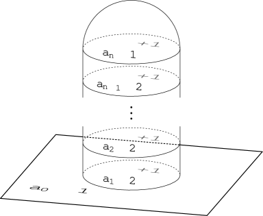
Figure 10. The shadow with no vertices corresponding to the surgeries on the chain in Figure 9. Intrinsically in the 4-manifold, this is equivalent to a chain of spheres, each intersecting the next in just one point.

With the notation of the figure, we glue $n$ copies of the polyhedron $H$ of Example 3.16 to $P_{1}$ so that one component of $\partial H_{1}$ is identified with $l_{1}$, $H_{j}$ is glued to $H_{j+1}$ and $H_{j-1}$ and the free component of $\partial H_{n}$ is a knot $l^{\prime}_{1}$. On the level of the boundary of the thickening we are gluing $n$ copies of the complement of the Hopf link in $S^{3}$ to $M$. Since the complement of the Hopf link is $T^{2}\times[0,1]$ the final 3-manifold is unchanged. But now the polyhedron $P^{\prime}_{1}=P_{1}\cup H_{1}\cup\ldots\cup H_{n}$ can be equipped with gleams so to describe the operation of Figure 9. The meridian $\mu^{\prime}_{1}$ of $l^{\prime}_{1}$ is now by construction the curve which, expressed in the initial base of $T_{1}$, is $a\lambda_{1}+b\mu_{1}$. Hence we can now glue $P^{\prime}_{1}$ and $P_{2}$ along $l^{\prime}_{1}$ and $l_{2}$ and choose suitably the gleam of the region of $P^{\prime}_{1}\cup P_{2}$ to obtain the desired homeomorphism. ∎

Corollary 3.28.

Shadow complexity is sub-additive under torus sums, i.e., under the gluing along toric boundary components through orientation reversing homeomorphisms.

One special case of torus sums is surgery, gluing in a solid torus. Surgery can decrease any reasonable notion of complexity, so shadow complexity cannot be additive under torus sums in general, hence we ask the following:

Question 3.29.

Let $M_{1}$ and $M_{2}$ be two oriented 3-manifolds with incompressible torus boundary components $T_{1}$ and $T_{2}$. Is it true that any torus sum of $M_{1}$ and $M_{2}$ along $T_{1}$ and $T_{2}$ has shadow complexity equal to $\operatorname{sc}(M_{1})+\operatorname{sc}(M_{2})$?

3.4. Complexity zero shadows

In this subsection we classify the manifolds having zero shadow complexity.

Definition 3.30.

An oriented 3-manifold is said to be a graph manifold if it can be decomposed by cutting along tori into blocks homeomorphic to solid tori and $R\times S^{1}$, where $R$ is a pair of pants (i.e., a thrice-punctured sphere).

Graph manifolds can also be characterized as those manifolds which have only Seifert-fibered or torus bundle pieces in their JSJ decomposition.

Proposition 3.31 (Complexity zero manifolds).

The set of oriented 3-manifolds admitting a shadow containing no vertices coincides with the set of oriented graph manifolds.

Proof..

To see that any graph manifold has a shadow without vertices, notice that a disk with boundary colored by $e$ is a shadow of a solid torus and, similarly, a pair of pants $R$ is a shadow of $R\times S^{1}$. Proposition 3.27 shows that any gluing of these blocks can be described by a shadow without vertices.

For the other direction, we must show that if a 3-manifold $M$ has a shadow $P$ without vertices, then it is a graph manifold. The polyhedron $P$ can be decomposed into basic blocks as follows. Since $P$ contains no vertices, a regular neighborhood of $\operatorname{Sing}(P)$ in $P$ is a disjoint union of blocks of the following three types:

1. the product of a $Y$-shaped graph and $S^{1}$;

2. the polyhedron obtained by gluing one boundary component of an annulus to the core of a Möbius strip; and

3. the polyhedron obtained by considering the product of a $Y$-shaped graph and $[-1,1]$ and identifying the graphs $Y\times\{1\}$ and $Y\times\{-1\}$ by a map which rotates the legs of the graph of $\frac{2\pi}{3}$.

Let $\pi:M\to P$ be the projection of $M$ on $P$. The complement of the above blocks in $P$ is a disjoint union of (possibly non-orientable) compact surfaces. The preimage under $\pi$ of each of these surfaces is a (possibly twisted) product of the surface with $S^{1}$ and hence is a graph manifold. Moreover, the preimage under $\pi$ of the above three blocks is a 3-dimensional sub-manifold of $M$ which admits a Seifert fibration (induced by the direction parallel to $\operatorname{Sing}(P)$) and hence is graph manifold. ∎

3.5. Decomposing shadows

In Proposition 3.31, we saw how to decompose a shadow with no vertices into elementary pieces. For more general shadows, we will need a new type of block. For simplicity, we will suppose that the boundary of $P$ is all marked “external” and that the singular set $\operatorname{Sing}(P)$ of the shadow $P$ is connected and contains at least one vertex. (This last can always be achieved by modifying $P$ with suitable local moves.) Let $P$ be a shadow for a 3-manifold $M$, possibly with non empty boundary, and let $\pi:M\to P$ be the projection. Then we have the following:

Proposition 3.32.

The combinatorial structure of $P$ induces through $\pi^{-1}$ a decomposition of $M$ into blocks of the following three types:

1. products $F\times S^{1}$ where $F$ is an orientable surface, or $F\mathbin{\tilde{\times}}S^{1}$ with $F$ non-orientable;

2. products of the form $R\times[-1,1]$, where $R$ is a pair of pants; and

3. genus 3 handlebodies.

Proof..

Decompose the polyhedron $P$ by taking regular neighborhoods of the vertices and then regular neighborhoods of the edges in the complement of the vertices. This decomposes $P$ into blocks of the following three types:

1. surfaces (corresponding to the regions);

2. pieces homeomorphic to the product of a $Y$-shaped graph and $[-1,1]$; and

3. regular neighborhoods of the vertices.

The preimage of the first of these blocks is a block of the first type in the statement. Let us consider the preimages of the products $Y\times[-1,1]$. The 4-dimensional thickening of one of these blocks is the product of the 3-dimensional thickening $\mathbf{Y}$ of the $Y$-graph and $[-1,1]$, where $\mathbf{Y}$ is a 3-ball containing a properly embedded copy of $Y$ and collapsing on it. The preimage in $M$ of this block is the product of $[-1,1]$ with $\partial{\mathbf{Y}}-\partial Y$, which is a pair of pants.

Let us denote by $V$ the simple polyhedron formed by a regular neighborhood of a vertex in $P$. We are left to show that $\pi^{-1}(V)$ is a genus 3-handlebody. The 4-thickening of $V$ is ${\mathbf{V}}\times[-1,1]$, where $\mathbf{V}$ is the 3-dimensional thickening of $V$, i.e., a 3-ball into which $V$ is properly embedded. In particular, $\partial V\subset\partial\mathbf{V}$ is a tetrahedral graph and so $\partial\mathbf{V}$ is split into four disks by $\partial V$. One can decompose $\partial({\mathbf{V}}\times[-1,1])$ as $\partial{\mathbf{V}}\times[-1,1]\cup\partial{\mathbf{V}}\times\{-1,1\}$. The part of this boundary corresponding to $M$ is the complement of $\partial V$ and is homeomorphic to ${\mathbf{V}}\times\{-1\}\cup(\partial{\mathbf{V}}-\partial V)\times[-1,1]\cup{\mathbf{V}}\times\{1\}$; this is composed of two 3-balls connected through 4 handles of index one (each of which corresponds to one of the four disks into which $\partial V$ splits $\partial\mathbf{V}$). ∎

Note that boundary the blocks of the second two types in Proposition 3.32 are themselves naturally decomposed into annuli and pairs of pants.

3.6. A family of universal links

Now suppose further that $P$ (and therefore $M$) has no boundary, and consider the union of the blocks of the second two types in Proposition 3.32. These two types of blocks meet in pairs of pants, and the remaining boundary is obtained from the annuli; therefore, we are left with a manifold $S_{P}$ with boundary a union of tori, which depends only on the polyhedron $P$ and not on the gleams. (The original manifold $M$ can be obtained by surgery on $S_{P}$.)

In this subsection we show that $S_{P}$ is a hyperbolic cusped 3-manifold whose geometrical structure can be easily deduced from the combinatorics of $P$. We furthermore show how to present $S_{P}$ as the complement of a link in a connected sum of copies of $S^{2}\times S^{1}$.

As before, let $P$ be a simple polyhedron (now with no boundary) such that $\operatorname{Sing}(P)$ is connected and contains at least one vertex; let $c(P)$ be the number of vertices. Let $S(P)$ be the regular neighborhood of $\operatorname{Sing}(P)$ in $P$, which we think of as a simple polyhedron with boundary colored “internal”. Let $l_{1},\ldots,l_{k}$ be the components of $\partial S(P)$ in $P$. To each $l_{i}$ we assign a positive integer number $c_{i}$ called its valence by counting the number of vertices touched by the region $R_{i}$ of $S(P)$ containing $l_{i}$ and an element of $\mathbb{Z}_{2}$ given by the $\mathbb{Z}_{2}$-gleam $g_{i}$ of the region of $S(P)$ containing $l_{i}$.

Let $X_{P}$ be the 4-thickening of $S(P)$ provided by Turaev’s Reconstruction Theorem; $X_{P}$ collapses onto a graph with Euler characteristic $\chi(S(P))=-c(P)$ and so $\partial X_{P}$ is a connected sum of $c(P)+1$ copies of $S^{2}\times S^{1}$. Moreover, $\partial S(P)$ is a link $L_{P}$ in $\partial X_{P}$. The manifold $S_{P}$ introduced earlier is the complement of $L_{P}$ in $\partial X_{P}$.

$S_{P}$ has a natural hyperbolic structure which we can understand in detail, as we will now see.

Proposition 3.33.

For any standard shadow surface $P$, $S_{P}$ can be equipped with a complete, hyperbolic metric with volume equal to $2v_{\mathrm{oct}}c$.

Proof..

The main point of the proof is to construct an hyperbolic structure on a block corresponding to a vertex in $S(P)$ and then to show that these blocks can be glued by isometries along the edges of $S(P)$.

Let us realize a block of type 3 as follows. In $S^{3}$, pick two disjoint 3-balls $B_{0}$ and $B_{\infty}$ forming neighborhoods respectively of 0 and $\infty$. Connect them using four 1-handles $L_{i}$, $i=1,\ldots,4$, positioned symmetrically, as shown in Figure 11.

In the boundary of the so obtained genus 3-handlebody consider the 4 thrice-punctured spheres formed by regular neighborhoods of the theta-curves connecting $B_{0}$ and $B_{\infty}$ each of which is formed by 3-segments parallel to the cores of three of the 1-handles. These four pants are the surfaces onto which the blocks of type 2 in Proposition 3.32 are to be glued. Indeed, these blocks are of the form $R\times[-1,1]$ where $R$ is a thrice punctured sphere, and they are glued to the blocks of type 3 along $R\times\{-1,1\}$. We will now exhibit an hyperbolic structure on this block so that these 4 thrice-punctured spheres become totally geodesic and their complement is formed by $6$ annuli which are cusps of the structure.

Consider a regular tetrahedron in $B_{0}$ whose barycenter is the center of $B_{0}$ and whose vertices are directed in the four directions of the 1-handles $L_{i}$. Truncate this tetrahedron at its midpoints as shown in Figure 11. The result is a regular octahedron $O_{0}$ contained in $B_{0}$, with 4 faces (called “internal”) corresponding to the vertices of the initial tetrahedron and 4 faces (called “external”) corresponding to the faces of the initial tetrahedron. Do the same construction around $\infty$ and call the result $O_{\infty}$. The handlebody $B_{0}\cup B_{\infty}\cup L_{i}$, $i=1,\ldots,4$ can be obtained by gluing the internal faces of $O_{0}$ to the corresponding internal faces of $O_{\infty}$. The remaining parts of the boundaries of the two octahedra are four spheres each with three ideal points and triangulated by two triangles. If we put the hyperbolic structure of the regular ideal octahedron on both $O_{0}$ and $O_{\infty}$, then, after truncating with horospheres near the vertices, we get the hyperbolic structure we were searching for: the geodesic thrice-punctured spheres come from the boundary spheres without their cone points and the annuli are the cusps of the structure. Each (annular) cusp has an aspect ratio of $\frac{1}{2}$ since it is the union of two squares, the sections of the cusps of an ideal octahedron near a vertex.

\psfrag{B_0}{$B_{0}$}\psfrag{B_infty}{$B_{\infty}$}\psfrag{l_1}{$L_{1}$}\psfrag{l_2}{$L_{2}$}\psfrag{l_3}{$L_{3}$}\psfrag{l_4}{$L_{4}$}\includegraphics[width=210.55022pt]{figure/hyperbolicstructure}

Figure 11. In this picture we show how to connect the two balls $B_{0}$ and $B_{\infty}$ in $S^{3}$ using the four legs $L_{i}$, $i=1,\ldots,4$. In the center of $B_{0}$, we visualize how the regular octahedron $O_{0}$ is embedded. In the figure, the four internal faces are directed towards the four legs of the handlebody since they are identified with the four internal faces of the octahedron $O_{\infty}$.

To show that these blocks can be glued and form a hyperbolic manifold $S_{P}$ it suffices to notice that the thrice-punctured spheres in a block of type 3 are all isometric. ∎

Proposition 3.34.

The Euclidean structure on the cusp corresponding to a boundary component $l_{i}$ of $S(P)$ is the quotient of $\mathbb{R}^{2}$ under the two transformations $(x,y)\cong(x+2,y)$ and, $(x,y)\cong(x+g_{i},y+c_{i})$.

Proof..

The cusp corresponding to $l_{i}$ is obtained by gluing some of the annular cusps in the blocks of the vertices: each time $l_{i}$ passes near a vertex $v$ of $S(P)$, we glue the annular cusp corresponding to $l_{i}$ in the block of $v$ (note indeed that in this block there are exactly $6$ cusps, one for each of the six regions passing near the vertex). Since each annular cusp has a section which is an annulus whose core has length 2 and height is 1, following $l_{i}$ and gluing the cusps corresponding to the vertices we meet, we construct an enlarging annular cusp; when we conclude a loop around $l_{i}$, we glued $c_{i}$ cusps and we got an annulus whose core has length 2 and whose height is $c_{i}$. Then, we are left to glue the two boundary components of this annulus to each other, and the combinatorics of $S(P)$ forces us to do that by applying $g_{i}$ half twists to one of the two components. ∎

Finally, we give a more explicit description of the link $L_{P}$ in terms of surgery on $S^{3}$.

Proposition 3.35.

$S_{P}$ can be presented as the complement of a link $L_{P}$ in the manifold obtained by surgering $S^{3}$ over a set of $c(P)+1$ unknotted 0-framed meridians (where $c(P)$ is the number of vertices of $P$). Moreover this link can be decomposed into blocks like those shown in Figure 12.

Proof..

Let $T$ be a maximal tree in $S(P)$ and consider its regular neighborhood, a contractible sub-polyhedron $P^{\prime}$ of $S(P)$; $S(P)$ can be recovered from $P^{\prime}$ by gluing to $P^{\prime}$ the blocks corresponding to the edges of $S(P)\setminus T$. Let $B$ be the 3-dimensional thickening of $P^{\prime}$, and let $X^{\prime}$ be $B\times[-1,1]$, the 4-dimensional thickening of $P^{\prime}$. The trivalent graph $\partial P^{\prime}$ is contained in $\partial B\times\{0\}\subset\partial X^{\prime}=S^{3}$. Moreover we can push $P^{\prime}$ into $\partial X^{\prime}$ by an isotopy keeping its boundary fixed. Then $\partial P^{\prime}$ is the boundary of a contractible polyhedron in $B^{3}$ and hence is composed by joining some copies of the blocks shown in the upper-left part of Figure 12 by means of triples of parallel strands. Each time we glue back to $P^{\prime}\subset X^{\prime}$ a block corresponding to an edge of $S(P)\setminus T$, we are gluing to $X^{\prime}$ a 1-handle connecting neighborhoods of two vertices, say $v_{1}$ and $v_{2}$, of $\partial P^{\prime}$. The boundary of the polyhedron we get that way is obtained from $\partial P^{\prime}$ by connecting the strands around $v_{1}$ and those around $v_{2}$ according to the combinatorics of $S(P)$ and letting it pass over the 1-handle once: this can be represented by a passage through a 0-framed meridian. Performing this construction on all the edges of $S(P)-T$ one gets the link $L_{P}$ of the form described in the statement. ∎

\psfrag{0}{$0$}\includegraphics[width=295.90848pt]{figure/blocchilink.eps}

\psfrag{0}{$0$}\includegraphics[width=239.00298pt]{figure/link.eps}

Figure 12. In the upper part of the picture we draw the basic blocks composing the links $L_{P}$. In the lower part we work out an example: at the left part we show an example of $S(P)$ (the curves represent $\partial S(P)$). In the right part we encircle the complement of a maximal tree of $\operatorname{Sing}(P)$ with 0-framed meridians.

As already noticed, any closed oriented 3-manifold has a shadow; moreover, up to applying some basic transformations to such a shadow, we can always suppose it to be standard. This has the following consequence:

Proposition 3.36.

The family of links $L_{P}$, with $P$ ranging over all standard polyhedra, is “universal”: any closed orientable 3-manifold can be obtained by a suitable integral surgery over an element of this family.

Since the number of standard polyhedra with at most $c$ vertices is finite, the family of universal links $L_{P}$ has a natural finite stratification given by the complexity of the polyhedron from which each element of the family is constructed. Using Jeff Weeks’ program SnapPea, we were able to check that all but 4 manifolds of the cusped census can be obtained by surgering over links corresponding to polyhedra with at most 2 vertices.

The following inequality from the introduction is a corollary of Gromov’s results [8]:

Theorem 3.37.

A 3-manifold $M$, with boundary empty or a union of tori, has shadow complexity of at least $(v_{\mathrm{tet}}/2v_{\mathrm{oct}})\|M\|$.

Proof..

In any shadow for $M$ with $n$ vertices, the preimage of a neighborhood of the singular set is the disjoint union of pieces which either have the hyperbolic structure described above (if there is at least one vertex in the connected component) or are graph manifolds (as in Proposition 3.31). The total Gromov norm of these pieces is therefore $(2v_{\mathrm{oct}}/v_{\mathrm{tet}})n$. $M$ can be obtained from these pieces by gluing some additional pieces from the regions: each region contributes a surface cross $S^{1}$. Since the Gromov norm is non-increasing under gluing along torus boundaries [8], $n$ must be at least $v_{\mathrm{tet}}/2v_{\mathrm{oct}}\cdot\|M\|$. ∎

Theorem 3.38.

A 3-manifold $M$ with Gromov norm $G$ has at least $G/10$ crossing singularities in any smooth, stable map $\pi:M\to\mathbb{R}^{2}$.

Proof..

Applying the construction underlying the proof of Theorem 4.2, one can construct $M$ as a Dehn filling of a link $L_{P}$ for a suitable simple polyhedron $P$; moreover, each singularity of the second type (as in Figure 18) produces a pattern which can be triangulated with $10$ regular ideal hyperbolic tetrahedra, and each singularity of the first type (as in Figure 16) can be obtained as the union of two regular ideal octahedra. Hence $M$ is the Dehn filling of an hyperbolic cusped 3-manifold whose volume is no more than $10s{v_{\mathrm{tet}}}$, where $s$ is the number of crossing singularities of $\pi$ and ${v_{\mathrm{tet}}}$ is the volume of the regular ideal tetrahedron. The statement follows. ∎

4. Shadows from triangulations

In this section, we exhibit a construction which, given a 3-manifold $M$ triangulated with $t$ tetrahedra (possibly with some ideal vertices), produces a shadow of the manifold containing a number of vertices bounded from above by $kt^{2}$ where $k$ is a constant which does not depend on $M$. This produces a 4-manifold whose shadow complexity (the least number of vertices of a shadow of the manifold) can be bounded by $kt^{2}$ and whose boundary is the given 3-manifold. Furthermore, we bound the gleam weight and the number of 4-simplices needed to construct the 4-manifold.

Because this is the central point of the paper, we go into some details and give an explicit estimate for $k$ and the bounds on the gleam weights.

From now on, by a triangulation we mean a $\Delta$-triangulation, an assembly of simplices glued along their faces, possibly with self-gluings.

Definition 4.1.

Let $M$ be an oriented 3-manifold whose boundary does not contain spherical components. A partially ideal triangulation of $M$ is a triangulation of the singular manifold $M/\partial M$ (obtained by identifying each boundary component to a point) whose vertices contain the singular points corresponding to the boundary components of $M$. An edge-distinct triangulation is a triangulation where the two vertices of each edge (simplex of dimension 1) are different.

This section is devoted to proving the following theorem which is the main tool in proving the results announced in the introduction:

Theorem 4.2.

Let $M$ is an oriented 3-manifold, possibly with boundary, and let $T$ be a partially ideal, edge-distinct triangulation of $M$ containing $t$ tetrahedra. There exists a shadow $P$ of $M$ which is a boundary-decorated standard polyhedron, contains at most $18t^{2}$ vertices, and has gleam weight at most $108t^{2}$.

Corollary 4.3.

With the assumptions an in Theorem 4.2, except that $T$ is not necessarily edge-distinct, then $M$ has a shadow which is a standard polyhedron, contains at most $24^{2}\cdot 18t^{2}$ vertices, and has gleam weight at most $24^{2}\cdot 108t^{2}$.

Proof..

Apply Theorem 4.2 to the barycentric subdivision of $T$, which has $24t$ tetrahedra and is edge-distinct. ∎

Proof of Theorem 4.2.

The main idea of the proof is to pick a map from $M/\partial M$ to $\mathbb{R}^{2}$, stabilize its singularities and associate to this map its Stein factorization, which turns out to be a decorated shadow of $M$. We split the proof of the theorem into 6 main steps.

1. Define an initial projection map. We map all the vertices to the boundary of the unit disk, so that they don’t interfere with the bulk of the construction.

2. Modify the projection map to get a map which is stable in the smooth sense. This involves modifying the projection in a neighborhood of the edges, in a uniform way along the edge.

3. Construct the shadow surface over the complement of a neighborhood of the codimension 2 singularities of the map. Here the shadow surface is just the Stein factorization as described in the introduction.

4. Extend the construction to the neighborhoods of the codimension 2 singularities. This involves analyzing the two interesting types of singularities. For one of the singularities we modify the Stein factorization slightly to get a shadow surface.

5. Estimate the complexity of the resulting shadow. Essentially, the vertices may come from interactions between a pair of edges, and there are quadratically many such interactions.

6. Estimate the gleams on the regions of the shadow.

4.1. The initial projection

Pick a generic map $\pi$ from the vertices $v_{1},\ldots,v_{n}$ of $T$ to the unit circle in $\mathbb{R}^{2}$ and call $p_{1},\ldots,p_{n}$ their images. Extend $\pi$ to all of $T$ in a piecewise-linear fashion to a map from $M/\partial M$ to the unit disk (see Figure 13). Pick a small disk around each $p_{i}$, and let $M^{\prime}$ be the complement in $M/\partial M$ of the preimage of these disks; $M^{\prime}$ is homeomorphic to $M$ minus a ball around each non-ideal vertex.

Let $G$ be the image (via $\pi$) in $\mathbb{R}^{2}$ of the union of the edges of $T$. If $p$ is any point in $\mathbb{R}^{2}\setminus G$ then $\pi^{-1}(p)$ is a set (possibly empty) of circles in $M^{\prime}$ since it is a union of segments properly embedded in the tetrahedra of $T$ never meeting the edges of $T$. We may think that the set of “critical values” of $\pi$ is contained in $G$.

\psfrag{v_1}{$v_{1}$}\psfrag{v_2}{$v_{2}$}\psfrag{v_3}{$v_{3}$}\psfrag{v_4}{$v_{4}$}\psfrag{p_1}{$p_{1}$}\psfrag{p_2}{$p_{2}$}\psfrag{p_3}{$p_{3}$}\psfrag{p_4}{$p_{4}$}\includegraphics[width=182.09746pt]{figure/projection1.eps}

Figure 13. In this figure we summarize the notation we fixed in the first step. The tetrahedron spanned from the vertices $v_{i}$ is a tetrahedron of the triangulation $T$ of $M/\partial M$.

4.2. A stable projection

The boundary of $M^{\prime}$ in $M/\partial M$ is a union of “vertical” surfaces, surfaces which project to segments of small circles around the points $p_{i}$. In the next sections we will restrict ourselves to $M^{\prime}$ and construct a Stein factorization of $\pi:M^{\prime}\to\mathbb{R}^{2}$, which turns out to be a shadow of $M^{\prime}$; we will then modify it to get a shadow for $M$.

The image of the edges $e_{i}$, $i=1,\ldots,r$ of $T$ form a set of segments $f_{i}$ in the unit circle. Since two edges $e_{i}$ and $e_{j}$ could have the same endpoints in $T$, some $f_{i}$ could coincide. To avoid this, we modify $\pi$ slightly around small regular neighborhoods of the edges in $M^{\prime}$ so that the projections of different edges with the same endpoints in $T$ are distinct segments in the unit circle running parallel to each other. This can be done by operating in disjoint small cylindrical neighborhoods of the edges, since no vertices of $T$ are contained in $M^{\prime}$. The resulting map is no longer PL.

Let us keep calling $G$ the graph which is the (modified) image of the $f_{i}$. The edges of $G$ are now straight segments away from neighborhoods of the $p_{i}$, with bends near the $p_{i}$. We now study the behavior of the projection map on a cylindrical regular neighborhood $C_{i}$ of each edge $e_{i}$ of $T$. Transverse to $e_{i}$ in $C_{i}$ is a triangulated disk with one interior vertex from $e_{i}$ and triangles coming from the tetrahedra of $T$ incident to $e_{i}$; the projection of this disk in $\mathbb{R}^{2}$ is a segment transverse to $f_{i}$. Let $\pi_{t}$ be the map from this transverse disk to the transverse segment. The map from $C_{i}$ to the neighborhood of $f_{i}$ is the product of $\pi_{t}$ with an interval, hence it suffices to study $\pi_{t}$.

For instance, consider the following possibility for $\pi_{t}$: let $Q$ be a square triangulated into four triangles by coning from the center, let $A$, $B$, $C$, $D$ be its vertices in cyclic order, and consider the PL map from $Q$ to $[-1,1]$ sending $A$ and $C$ to $1$, $B$ and $D$ to $-1$ and the center to $0$. The preimage of a point near $1$ (resp. $-1$) is a pair of segments near $A$ and $C$ (resp. $B$ and $D$). The preimage of $0$ is the cone from the center of $Q$ to the midpoints of its edges. This map is the typical example of a saddle on the base of $C_{i}$.

If we repeat the above construction with an hexagon, sending the vertices alternately to 1 and $-1$, we obtain instead a “monkey saddle”, which is not stable (from the smooth point of view). The inverse image of 0 is a cone over the midpoints of the edges from the center: a six-valent star. As shown in Figure 14, in this case $\pi_{t}$ can be perturbed to a map having two stable critical points as shown in the figure. In general, if the inverse image of a critical value is a star with $2k$ legs, then $\pi_{t}$ can be perturbed to a map containing $k-1$ stable saddle points all having distinct images in the segment.

There is one case left: when the whole disk is projected on one side of 0 in $[-1,1]$. In this case the singular point in the center of the disk is an extremum and we keep the map unchanged.

\psfrag{Preimage of zero}{Preimage of zero}\psfrag{Preimage of -1/2}{Preimage of $-1/2$}\psfrag{Preimage of 1/2}{Preimage of $1/2$}\psfrag{1}{$1$}\psfrag{-1}{$-1$}\includegraphics[width=210.55022pt]{figure/stabilization.ps}

$\vbox{\hbox{\includegraphics[trim=-1.00374pt -1.00374pt -1.00374pt -1.00374pt]{draws/surface.80}}}\longrightarrow\vbox{\hbox{\includegraphics[trim=-1.00374pt -1.00374pt -1.00374pt -1.00374pt]{draws/surface.81}}}$

Figure 14. Stabilizing the map sending the vertices of an hexagon over $[-1,1]$ alternatively in $\pm 1$. In the right part we show the preimages of the two singular values ($\pm\frac{1}{2}$) of the stabilized map. The lower diagram is another representation, where the projection to $\mathbb{R}$ is the projection onto the vertical axis.

We now modify $\pi:C_{i}\to\mathbb{R}^{2}$ as above around each edge $e_{i}$ to get the cylinder of a stable map from a disk to a segment. This increases the set of critical values of $\pi$ near $f_{i}$ so that it no longer coincides with $f_{i}$, but is formed by a set of strands running parallel to it, all corresponding to stable singularities of the map. Let us keep calling $G$ the graph in $\mathbb{R}^{2}$ made of these critical values; as before, it consists of straight segments away from the vertices $p_{i}$, with bent segments near the $p_{i}$. These straight segments are cut by their intersections $x_{k},\ k=1,\ldots,l$ (which, together with the points $p_{i}$, form the vertices of $G$) into sub-segments $h_{j},j=1,\ldots,m$ (which form the edges of $G$).

4.3. The Stein factorization away from codimension 2 singularities

Pick a regular neighborhood of each vertex of $G$, and let $M^{\prime\prime}$ be the preimage through $\pi$ of the complement of these neighborhoods. We will now construct a shadow $P^{\prime\prime}$ for $M^{\prime\prime}$ from the Stein factorization for the map $\pi$, as shown in Figure 15.

Let $R_{1}$, …, $R_{m}$, $R_{\infty}$ be the connected components of $\mathbb{R}^{2}\setminus G$, where $R_{\infty}$ is the unbounded region and $R_{i}$, $i\neq\infty$, are disks. By construction, $\pi^{-1}(R_{\infty})$ is empty and $\pi^{-1}(R_{i})$, $i\neq\infty$ is a disjoint union of $n_{i}$ open solid tori in $M^{\prime}$. For an edge $h_{j}$ of $G$, let $\alpha_{j}$ be a small arc intersecting it transversally and connecting two regions, say $R_{0}$ and $R_{1}$. Let $q_{0}$ and $q_{1}$ be the endpoints of $\alpha_{j}$; the (possibly disconnected) surface $S_{j}=\pi^{-1}(\alpha_{j})\subset M^{\prime\prime}$ is the cobordism between $\pi^{-1}(q_{0})$ and $\pi^{-1}(q_{1})$ whose possible shapes are depicted in Figure 15.

To construct the Stein factorization of $\pi$, for each $R_{i}$, take $n_{i}$ copies of $R_{i}$. We need to connect these regions to each other near the centers of the segments $h_{j}$. To do this, we apply the procedure of Figure 15, where all the possible behaviors of $S_{j}$ are examined. Saddle singularities produce a singular set in the polyhedra used to connect the regions. Shrinking singularities (when the transverse map $\pi_{t}$ in the previous step maps entirely on one side of the singularity) produce a boundary segment of $P^{\prime\prime}$, which we mark as “false”; temporarily mark the rest of the boundary of $P^{\prime\prime}$ as “internal”. Call the regions which are involved in the singularity or boundary over $h_{j}$ the interacting regions.

\psfrag{R_1}{$R_{1}$}\psfrag{R_2}{$R_{2}$}\psfrag{f_1}{$f_{1}$}\psfrag{f_2}{$f_{2}$}\psfrag{Singular values}{Singular values}\psfrag{P}{$P$}\psfrag{Sing(P)}{$\operatorname{Sing}(P)$}\psfrag{pigreco'}{$\pi_{1}$}\psfrag{pigrecop}{$\pi_{2}$}\psfrag{R_1^i}{$R_{1}^{i}$}\psfrag{R_1^j}{$R_{1}^{j}$}\psfrag{R_1^k}{$R_{1}^{k}$}\psfrag{R_1^l}{$R_{1}^{l}$}\psfrag{R_2^i}{$R_{2}^{i}$}\psfrag{R_2^j}{$R_{2}^{j}$}\includegraphics[width=352.814pt]{figure/projection2.eps}

Figure 15. The construction we perform in Step 3. To each fiber over a region of $\mathbb{R}^{2}$ we associate a region of $P^{\prime\prime}$. We glue these regions along their boundaries to the type of singularity which intervenes. In the highest part of the picture we see the simplest case: when the singularity does not affect the fibers corresponding to two regions of $P^{\prime\prime}$. The second case is the one of a shrinking singularity, which creates a false boundary component in $P^{\prime\prime}$. The last case is the case of a simple saddle singularity, which creates an arc in $\operatorname{Sing}(P^{\prime\prime})$.

If we repeat the above construction for all pairs of regions in contact through a segment of the family $h_{j}$, we get a decorated simple polyhedron which represents the Stein factorization of $\pi:M^{\prime\prime}\to\mathbb{R}^{2}$. We can naturally find maps $\pi_{1}:M^{\prime\prime}\to P^{\prime\prime}$ and $\pi_{2}:P^{\prime\prime}\to\mathbb{R}^{2}$ so that $\pi=\pi_{2}\circ\pi_{1}$.

Let us analyze $\partial_{e}P^{\prime\prime}$. Currently, $\pi_{2}(P^{\prime\prime})$ covers the complement in $\mathbb{R}^{2}$ of small circular neighborhoods of the vertices of $G$, which are either the points $p_{i}$ (the images of the vertices of $T$) or intersections $x_{k}$ of the edges $f_{i}$. The inverse image in $P^{\prime\prime}$ of the boundaries of these circular neighborhoods is $\partial_{e}P^{\prime\prime}$, which is a trivalent graph possibly with some free ends.

4.4. Codimension-2 singularities

We now describe how to extend $P^{\prime\prime}$ to get a shadow $P^{\prime}$ of $M^{\prime}$. We fill in the gaps of the polyhedron near the intersections $x_{k}$ of critical values by using a simple polyhedron with at most 2 vertices per intersection.

Near each $x_{k}$ two segments of critical values intersect, say $s_{1}$ and $s_{2}$. For every region which is not interacting over either $s_{1}$ or $s_{2}$, we fill in the hole over $x_{k}$ with a disk. Also, if the region(s) interacting over $s_{1}$ do not meet those interacting over $s_{2}$, we can fill in the hole with the same simple blocks as in Figure 15 without adding any new vertices. In particular this always occurs if the singularity over $s_{1}$ or $s_{2}$ is a shrinking singularity.

We are left with the case when both $s_{1}$ and $s_{2}$ correspond to saddle singularities. In this case the component of the preimage $\pi^{-1}(x_{k})$ containing the singularities is a connected 4-valent graph $F$ in $M^{\prime}$ with two vertices, one from each singular segment. The edges of $F$ are oriented: At a generic point on an edge of $F$, a small disk in $M^{\prime}$ transverse to the edge maps homeomorphically to its image in $\mathbb{R}^{2}$ and so we can pull back the orientation of $\mathbb{R}^{2}$ to it. Then, since $M^{\prime}$ is oriented, we can orient the edges of $F$. Each vertex of $F$ corresponds to a codimension 1 singularity whose singular values are contained either in $s_{1}$ or in $s_{2}$. Moreover, near each vertex of $F$, two edges are incoming and the other two outgoing. Therefore the only possibilities for $F$ are these graphs:

$$\vbox{\hbox{\includegraphics[trim=-1.00374pt -1.00374pt -1.00374pt -1.00374pt]{draws/singularity.5}}}\textrm{\quad or\quad}\vbox{\hbox{\includegraphics[trim=-1.00374pt -1.00374pt -1.00374pt -1.00374pt]{draws/singularity.51}}}.$$

While passing through the codimension 1 singularity corresponding to a vertex, the edges of $F$ recouple so that incoming edges are glued to outgoing edges.

We now analyze these two cases and show that if $F=\pi^{-1}(x_{k})$ has the first shape, then its neighborhood in $M^{\prime}$ can be reconstructed by using a shadow polyhedron with one vertex, while in the second case, two vertices are sufficient. In both cases, the regular neighborhood of $F$ in $M^{\prime}$ is a 3-handlebody $H(F)$. By construction, the boundary $\Sigma_{3}$ of this handlebody projects, through $\pi_{1}$, to a component $G$ of $\partial_{i}P^{\prime\prime}$ and, through $\pi$, to a circle in $\mathbb{R}^{2}$ which is the boundary of a small regular neighborhood of $x_{k}$. The thickening of $G$, contained in the thickening of $P^{\prime\prime}$ constructed so far, is another 3-handlebody $H(G)$ lying vertically (through $\pi_{2}$) over this circle, and whose boundary is identified in $M^{\prime}$ with $\Sigma_{3}$. We will show that in both cases the union of these two handlebodies is $S^{3}$ and then construct a shadow of $(S^{3},G)$, where $G$ is considered as a subset of $H(G)\subset S^{3}$.

Case 1. $F$ is  .

Figure 16. The behavior over a neighborhood $U$ of the intersection of two segments  $s_{1}$, $s_{2}$ of singular values of the projection map when the singular graph $F=\pi^{-1}(x_{k})$ is  . We see the different topological types of preimages of points, with the induced orientation. The different types of points are the four regular areas (the components of $U\setminus(s_{1}\cup s_{2})$), the segments $s_{1}$ and $s_{2}$ themselves, and the intersection $s_{1}\cap s_{2}$. We have marked two different systems of curves in the fibers. One (the $n_{i}$) are copies of the fibers over the upper right region; these are meridians for $H(G)$. The other (the $m_{i}$) map surjectively to $\partial U$, and are meridians for $H(F)$. In the picture they appear as a choice of one point in each fiber.

In Figure 16, we show the preimages in $M^{\prime}$ of various points in a small circular neighborhood $U$ of $x_{k}$ in $\mathbb{R}^{2}$. In each component of $U\setminus(s_{1}\cup s_{2})$ the preimage of a point is a union of circles in $M^{\prime}$. While crossing $s_{1}$ or $s_{2}$ two arcs of these circles approach each other and after passing through a singular position, they recouple. In the figure, we show the preimage of a point in each of the regular areas and on each of the singularities.

In the figure we have picked three of the edges of $F$. Transverse to these edges are three meridian disks of $H(F)$ bounded by curves $m_{1}$, $m_{2}$ and $m_{3}$. Each disk can be chosen to be a section of $\pi$ as shown by the dots in Figure 16, so that each of the $m_{i}$ projects homeomorphically to $\partial U$.

We now identify meridians of $H(G)$. By construction, each circle in $M^{\prime}$ which is in the preimage of a regular point in $\mathbb{R}^{2}$ bounds a disk in $H(G)$: the preimage of the corresponding point in the thickening of $P^{\prime\prime}$. Hence the meridian curves of $H(G)$ include the circles drawn in Figure 16 over the 4 areas near $x_{k}$. In the upper-right region the preimage of a point is composed of three circles $n_{1},n_{2}$ and $n_{3}$, which we can choose as our Heegaard system.

The handlebodies $H(F)$ and $H(G)$ are glued along their boundaries. Since each meridian $n_{i}$ of $H(G)$ intersects exactly one time one of the meridians $m_{j}$ of $H(F)$, we have $H(G)\cup H(F)=S^{3}$. Inside this 3-sphere, $G$ is a 3-valent graph. The vertex of Figure 5, with boundary colored $i$, forms a shadow of the pair $(S^{3},G)$: Its thickening is $B^{4}$ and its boundary sits in $S^{3}=\partial B^{4}$. To see that this is a correct shadow, in Figure 17, we exhibit two oriented graphs embedded in $S^{3}$ which are homeomorphic respectively to $G$ and $F$. Moreover, the graphs are equipped with systems of meridians $n_{i}$ and $m_{i}$, respectively; when the meridians are homotoped into a common surface, the intersections $m_{i}\cap n_{j}$ coincide with the corresponding intersections in $M^{\prime}$ between the meridians of $H(F)$ and $H(G)$.

This shows that, when the codimension two singularity is , it is sufficient to form $P^{\prime}$ by gluing one vertex to $P^{\prime\prime}$ in order to extend the description of $M^{\prime}$ over $x_{k}$.

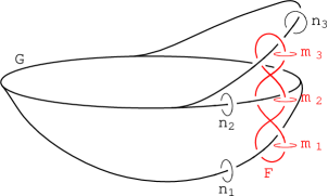
Figure 17. The two graphs $G$ (in black) and $F$ (in red) embedded in $S^{3}$. Their thickenings form two genus 3 handlebodies in $S^{3}$ equipped with meridian curves whose intersections agree with the intersections of the curves $m_{i}$ and $n_{i}$ described in the text.

Case 2. $F$ is  .

For this case, Figure 18 shows the preimages in $M^{\prime}$ of various points in a small neighborhood of $x_{k}$. As shown in the figure, two opposite areas are covered by 2 circles and the other two by 1 circle.

Figure 18. The same analysis as in Figure 16, in the case when the singular fiber is  . The $m_{i}$ are the meridian curves of $H(F)$ and the $n_{i}$ are the meridian curves of $H(G)$.

Let us choose a set of meridian curves $m_{1}$, $m_{2}$, $m_{3}$ for $H(F)$, as shown in Figure 18. For $H(G)$ we pick three curves $n_{1}$, $n_{2}$, $n_{3}$ out of those lying over the two areas covered by two circles: they form an Heegaard system for $H(G)$ since they bound disks in it and do not disconnect $\partial H(G)$. Then the number of intersections between the $m_{i}$ and the $n_{i}$ is as follows:

m_i ∩n_j n_1 n_2 n_3

vhv m_1 1 0 1

m_2 1 0 0

m_3 0 1 0

Hence we can reduce the Heegard diagram to the trivial diagram by eliminating in turn the pairs $(m_{3},n_{2})$, $(m_{2},n_{1})$, and $(m_{1},n_{3})$. This shows that in this case as well $H(G)\cup H(F)=S^{3}$, with embedded graphs $G$ (from $\partial_{i}P^{\prime\prime}$) and $F$ (from $\pi^{-1}(x_{k})$). In Figure 19 we show how these graphs and the corresponding meridians are embedded in $S^{3}$.

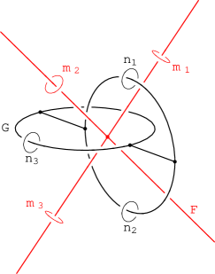
Figure 19. Two graphs in $S^{3}$ forming two genus 3 handlebodies whose union is the whole space and whose indicated meridians intersect as the curves $n_{i}$ and $m_{i}$ do. The legs of the red graph $F$ meet in an additional point at $\infty$.

Now that we know the position of $G$ in $S^{3}$, we are left to construct a simple polyhedron with boundary describing the pair $(S^{3},G)$. We saw in Example 3.17 that this graph is represented by the shadow in Figure 20. Therefore in this case to extend the construction of the shadow of $M^{\prime}$ to the singularities of codimension 2 it is sufficient to use a polyhedron with two vertices.

Figure 20. The polyhedron (containing only two vertices) we use to complete the construction of $P^{\prime}$ near the codimension 2 singularities of the second type. The boundary of the polyhedron (thicker in the picture) coincides with the boundary of the polyhedron $P^{\prime\prime}$ already constructed away from the singularity.

4.5. Shadow complexity estimate

In the preceding steps, we constructed a shadow surface $P^{\prime}$ for $M^{\prime}$, together with maps $\pi_{1}:M^{\prime}\to P^{\prime}$ and $\pi_{2}:P^{\prime}\to\mathbb{R}^{2}$ providing the Stein factorization of $\pi:M^{\prime}\rightarrow\mathbb{R}^{2}$. Let us now show that the total number of vertices in this shadow is bounded by a constant times $t^{2}$, where $t$ is the number of tetrahedra in the initial triangulation $T$.

Given an edge $e_{i}$ of $T$, let $v(e_{i})$ be the valence of $e_{i}$, i.e., the number of tetrahedra in $T$ containing $e_{i}$. If $e_{i}$ is contained twice in a tetrahedron we count it twice. Since each tetrahedron has $6$ edges, we have

$$\sum_{i}v(e_{i})=6t.$$

Let us now count the total number of segments of singular values in $\mathbb{R}^{2}$ (i.e., the number of $f_{i}$). In Step 2, while perturbing $\pi$ near an edge $e_{i}$ in order to get a stable map, we obtain at most $\frac{v(e_{i})}{2}-1$ segments of critical values. Thus the total number of $f_{i}$ is less than $\sum_{i}\frac{v(e_{i})}{2}=3t$. Then, the number of vertices in $P^{\prime}$ is bounded by $2(\#\{f_{i}\})^{2}\leq 18t^{2}$ since each vertex or pair of vertices comes from a crossing.

So the above construction produces a polyhedron $P^{\prime}$ with boundary having a well-controlled number of vertices and admitting a 4-thickening $W_{P^{\prime}}$ whose boundary contains $M^{\prime}$. We claim that the regions of $P^{\prime}$ are disks. To see this, note that the regions project by $\pi_{2}$ locally homeomorphically onto $\mathbb{R}^{2}$ (since the points in $P^{\prime}$ where $\pi_{2}$ is not locally a homeomorphism are, by construction, $\operatorname{Sing}(P^{\prime})$). Furthermore, by examining Figures 16 and 18, we see that the boundary of the projection of each region turns only to the left (with the induced orientation from $\mathbb{R}^{2}$). Then for each region of $P^{\prime}$ apply the following lemma.

Lemma 4.4.

Let $R$ be a connected oriented surface with boundary and $\pi:R\to\mathbb{R}^{2}$ be a local orientation-preserving homeomorphism so that $\pi|_{\partial R}$ turns to the left. Then $R$ is a disc and $\pi$ is an embedding.

Proof..

Define the straight arcs in $R$ to be the curves which are locally projected into straight arcs in $\mathbb{R}^{2}$; observe that $\pi$ is injective on a straight arc. Let $p$ be an interior point of $R$. We claim that the set of points which can be connected to $p$ by a straight arc is all of $R$: this clearly implies the statement. If this set were not open then one could find a straight arc connecting $p$ to another point $q$ whose projection is tangent internally to $\pi(\partial R)$ but this is ruled out by local convexity of the image. On the other hand, because the limit of a sequence of rays is itself a ray, this set is also closed and so is all of $R$. ∎

Let us now color each edge of $\partial P^{\prime}$ with one of the colors $e$ (“external”) and $f$ (“false”), the “false” edges being those produced during Step 3 of the construction (corresponding to shrinking circles in $M^{\prime}$) and the “external” edges being the remaining ones (around the vertices $p_{i}$). Then $P^{\prime}$ is a shadow for $M^{\prime}$, and $M^{\prime}$ sits inside the boundary of the thickening $W_{P^{\prime}}$ of $P^{\prime}$ as the union of the horizontal boundary (i.e., $\pi_{1}^{-1}(\operatorname{int}P^{\prime})$) and the vertical boundary over $\partial_{f}P^{\prime}$ (i.e., $\pi_{1}^{-1}(\partial_{f}P^{\prime})$). The components of $\partial M^{\prime}$ are surfaces $S_{i}$ that map through $\pi$ to the boundaries of small circles around the $p_{i}$. By Remark 3.13, each spherical component of $\partial M^{\prime}$ corresponds to a contractible component of $\partial_{e}P^{\prime}$ whose preimage through $\pi_{1}$ in $\partial W_{P^{\prime}}$ is a 3-ball.

Recall that $M^{\prime}$ is homeomorphic to $M$ minus a neighborhood of each non-ideal vertex of $T$. Hence, to get a shadow $P$ for $M$, it is sufficient take $P^{\prime}$ with the boundary components corresponding to these non-ideal vertices marked as false.

This concludes the construction of a decorated shadow $P$ for $M$ and an estimate of its shadow complexity.

4.6. Gleam estimate

We now provide an upper bound for the absolute value of the gleam of a region $D$ of $P$. We remark first of all that if the closure $\overline{D}$ of $D$ intersects $\partial_{f}P$, then no gleam has to be defined on $D$, as the gleam is defined only on the interior regions of $P$. Note that, by Lemma 4.4, $\overline{D}$ is a closed disc in $P$ with $\partial\overline{D}\subset\operatorname{Sing}(P)$. Let $v_{1},\ldots,v_{n}$ and $e_{1},\ldots,e_{n}$ be respectively the vertices and the edges of $\operatorname{Sing}(P)$ contained in $\partial\overline{D}$ so that $\partial e_{i}=v_{i+1}\cup v_{i}$. Let $B$ be a “shrunk copy of $\overline{D}$”, that is, the complement in $\overline{D}$ of a small open neighborhood of $\partial\overline{D}$. Equip $\partial B$ with the decomposition into vertices $w_{i}$ and edges $f_{i}$ induced by that of $\partial\overline{D}$.

Now we lift $e_{i}$ to the strand $e^{\prime}_{i}\subset M$ of singular points of $\pi$ such that $\pi_{1}(e^{\prime}_{i})=e_{i}$. This allows us to also choose lifts $f^{\prime}_{i}$ of $f_{i}$ by considering the points in $\pi_{1}^{-1}(f_{i})$ which are nearest to $e^{\prime}_{i}$. Notice that over some $f_{i}$, we could have two choices for $f^{\prime}_{i}$ according to how $D$ is positioned with respect to the saddle singularity corresponding to $e_{i}$. To get a section of $\pi_{1}$ over $\partial B$ we need to choose how to connect the endpoints of the $f^{\prime}_{i}$ with curves in $\pi_{1}^{-1}(w_{i})$. But $w_{i}\notin\operatorname{Sing}(P)$ and so $\pi_{1}^{-1}(w_{i})$ is an oriented curve, so we connect the endpoints of $f^{\prime}_{i}$ and $f^{\prime}_{i-1}$ through an oriented arc over $w_{i}$. With an appropriate choice of these arcs over $w_{i}$, a section $s_{B}$ of $\pi_{1}$ over $\partial B$ corresponds to that used in Proposition 3.6 to compute the gleam.

We now construct a section $B^{\prime}$ of $\pi_{1}$ over $B$. To do this, let $T^{(1)}$ be the $1$-skeleton of $T$ and for each component $B_{i}$ of $B\setminus\pi_{1}(T^{(1)})$ choose a face $F_{i}$ of $T$ so that $B_{i}\subset\pi_{1}(F_{i})$ and let $B^{\prime}_{i}=\pi_{1}^{-1}(D_{i})\cap F_{i}$. One can choose the faces so that they fit coherently on the edges of $T$ projecting inside $B$, because, by construction, these edges correspond to non-critical points. The union of the $B^{\prime}_{i}$ is $B^{\prime}$.

Now compare the section $s_{B}$ with $\partial B^{\prime}$ by counting $\#\{s_{B}\cap\partial B^{\prime}\}$. Note that, over an edge $f_{i}$, $s_{B}$ and $\partial B^{\prime}$ run parallel to each other (because the singular points of $\pi$ are by construction parallel to the edges of $T$). We claim that near a vertex $w_{i}$ they intersect at most once. Indeed, by construction $s_{B}$ is an embedded arc in $\pi_{1}^{-1}(v_{i})$ whose endpoints are the two endpoints of the lifts $f^{\prime}_{i}$ and $f_{i-1}$. On the other side, near $w_{i}$, $B^{\prime}$ is formed by a face $F$ of $T$ and at most one of $f^{\prime}_{i}$ and $f^{\prime}_{i-1}$ can be near to an edge of $F$ so $\partial B^{\prime}$ can stay near to at most one of $e^{\prime}_{i}$ and $e^{\prime}_{i-1}$. So, the two sections can intersect over $w_{i}$ but they can do it at most once.

Therefore the total gleam of $D$ is bounded above by the number of vertices in $\partial\overline{D}$ and, since each vertex of $P$ touches exactly $6$ regions, then the gleam weight of $P$ is at most $6\cdot 18\cdot t^{2}$. This concludes the proof of Theorem 4.2. ∎

5. Upper bounds

We can now apply our main tool on constructing shadows, Theorem 4.2, to give upper bounds on the complexity of various representations of 3-manifolds in terms of geometric properties.

5.1. Triangulating the 4-manifold

We now turn to the proof of Theorem 5.2, that 3-manifolds efficiently bound 4-manifolds. To actually construct the triangulated 4-manifold, we use the following:

Lemma 5.1.

Let $(P,g)$ be a boundary-decorated shadow with $n$ vertices whose regions are disks. There exists a triangulation of the manifold $W_{P}$ obtained by thickening $(P,g)$ (as described by Turaev’s Reconstruction theorem) containing $O(n+|g|)$ simplices. Moreover, the triangulation can be chosen so that the number of simplices touching each vertex is bounded above by a constant not depending on $P$ or $g$.

Proof..

Choose a triangulation of $P$ such that $\operatorname{Sing}(P)$ is composed of simplices, the number of simplices depends linearly (through a constant independent of $P$) on $n$, and the number of simplices touching each vertex of the triangulation is bounded above by a constant independent of $P$. Let $P^{\prime}$ be the triangulated polyhedron obtained by deleting a triangle from each region of $P$ and let $L$ be a 3-dimensional thickening of $P^{\prime}$ (which may be non-orientable). By gluing prisms on each triangle of $P^{\prime}$ one can construct a triangulation of $L$ containing at most $k$ simplices, where $k=O(n)$. Similarly, the number of simplices touching a vertex can be linearly bounded from above by a fixed constant not depending on $(P,g)$.

The 4-dimensional thickening $W_{P^{\prime}}$ (note that $P^{\prime}$ has no internal region and hence no gleam is needed to thicken it) is a fiber bundle over $L$ with fiber $[-1,1]$. This bundle is the unique bundle whose total space is orientable, so $W_{P^{\prime}}$ can be triangulated with a number of simplices bounded above by $6k$, since $6$ is the minimal number of simplices needed to triangulate the product of $[-1,1]$ and a 3-dimensional tetrahedron. Note that the part of the boundary of $W_{P^{\prime}}$ which collapses onto the boundary components of $\partial P^{\prime}$ that correspond to the triangular punctures is a set of solid tori $T_{i}$, all equipped with the same triangulation. In particular, let $s$ be the number of 3-simplices in the triangulation of each of these tori. Applying a Dehn twist to a meridian of a solid torus $T_{i}$, one obtains a new triangulation of $T_{i}$ which can be connected by means of, say, $m$ standard moves of triangulations (called “Pachner moves”) to the initial one. Each Pachner move corresponds to gluing a 4-dimensional simplex to $T_{i}$ along a face and looking at the new triangulation induced on $T_{i}$ by the new faces of the simplex. Hence, in order to perform $g_{i}$ Dehn twists on $T_{i}$ it is sufficient to glue $mg_{i}$ 4-simplices to $W_{P^{\prime}}$. Then, gluing a 2-handle on $T_{i}$ (which can be triangulated with a number of simplices depending only on $s$) produces a triangulated version of $W_{P}$.

By construction, the number of simplices of dimension 4 in this triangulation is bounded above by a constant times the number of simplices in the triangulation of $P^{\prime}$ plus the sum over all the regions of $P$ of $s+|g_{i}|$ where $g_{i}$ are the gleams and $s$ is the number of simplices on the solid tori $T_{i}$. Moreover, the number of simplices touching any vertex of the so obtained triangulation can be controlled from above by a suitable constant which does not depend on $(P,g)$. ∎

Theorem 4.2 and Lemma 5.1 together prove one main result:

Theorem 5.2.

If a 3-manifold $M$ has a triangulation with $t$ tetrahedra, then there exists a 4-manifold $W$ such that $\partial W=M$ and $W$ is triangulated with $O(t^{2})$ simplices. Moreover, $W$ has “bounded geometry”, that is, there exists an integer $c$ (not depending on $M$ and $W$) such that each vertex of the triangulation of $W$ is contained in less than $c$ simplices.

An alternate construction gives a simply-connected 4-manifold.

Theorem 5.3.

A 3-manifold with a triangulation with $k$ tetrahedra is the boundary of a simply-connected 4-manifold with $O(k^{2})$ 4-simplices.

Proof..

Applying the construction underlying the proof of Theorem 4.2 to the 3-manifold $M$, we produce a decorated shadow $P$ of $M$ whose singular set projects to $\mathbb{R}^{2}$, which contains $O(k^{2})$ vertices and whose regions are discs. Note that furthermore that the projection of the singular set has $O(k^{2})$ self-intersections. Collapse the false boundary of $P$ and appropriately modify the result to get a genuine simple shadow of $M$ with no more vertices as in Remark 3.19; the result may not be a standard polyhedron, but we can modify it to get a standard polyhedron with local moves. The result is a standard polyhedron, which we continue to call $P$, which still has a map to $\mathbb{R}^{2}$ with at most $O(V^{2})$ vertices.

Now apply Proposition 3.35 to $P$. The resulting hyperbolic link $L_{P}$ is obtained by gluing the pieces as in Figure 12 and performing surgery on some 0-framed meridians. Using the projection to $\mathbb{R}^{2}$, we get a link diagram with 1 crossing per vertex of $P$, at most 3 crossings per edge of $P$, 9 crossings per crossing of the projection of edges of $P$, and 6 crossings per 0-framed meridian: $O(k^{2})$ crossings in all. $M$ can be obtained by integer surgery on this link with coefficients related to the gleams, and so bounded by $O(k^{2})$. This surgery diagram therefore gives a simply-connected 4-manifold whose boundary is $M$ with complexity $O(k^{2})$. ∎

Note that the proof of Theorem 5.3 depended on a reasonably nice projection from the shadow to the plane; in general, there is no reason to believe that a shadow can be turned into a simply-connected shadow without an increase in complexity.

5.2. Upper bounds from geometry

We now turn to hyperbolic geometry, and prove various upper bounds based on geometry, including an estimate for the shadow complexity of a hyperbolic 3-manifold by the square of its Gromov norm.

We first recall an estimate for the number of tetrahedra in a triangulation from the hyperbolic volume.

Theorem 5.4 (W. Thurston).

There is a positive constant $C$ so that, for every hyperbolic 3-manifold $M$, there is a link $L$ contained in $M$ and a partially ideal triangulation of $M\setminus L$ with less than $C\cdot\operatorname{Vol}(M)$ tetrahedra.

This theorem was first used in the proof of the Thurston-Jørgensen Theorem [36, Theorem 5.11.2]. We recall the proof here.

Proof..

Let $V(r)$ be the volume of a ball of radius $r$ in $\mathbb{H}^{3}$.

Let $c$ be the Margulis constant, and consider the thick-thin decomposition of $M$: let $\varepsilon=c/2$, and let $M^{\prime}$ be the $\varepsilon$-thick part of $M$; we will take $L$ to be the core of $M\setminus M^{\prime}$. Consider a generic maximal $\varepsilon$-net in $M^{\prime}$, i.e., a maximal set of points $p_{i}$ such that the distance between any two of them is at least $\varepsilon$. Then the balls of radius $\varepsilon$ around the $p_{i}$ cover $M^{\prime}$ and the balls of radius $\varepsilon/2$ around the $p_{i}$ are embedded in $M$. Therefore the number of $p_{i}$ is bounded above by $\operatorname{Vol}(M)/V(\varepsilon/2)$. Starting from this $\varepsilon$-net we can construct a triangulation $T$ of a manifold homeomorphic to $M^{\prime}$ by taking the Delaunay triangulation of the $p_{i}$; that is, a set of $p_{i}$ are in a simplex of $T$ exactly when there is a point $x$ in $M^{\prime}$ which is equidistant from the chosen $p_{i}$ (and no farther than $\varepsilon$ from them) and no closer to any other $p_{i}$. Since the $p_{i}$ were chosen to be generic, this is actually a triangulation.

To estimate the number of tetrahedra in $T$, let us consider the lift $\tilde{T}$ of $T$ to $\mathbb{H}^{3}$. Note that two vertices that are connected by an edge have distance at most $2\varepsilon$, and so balls of radius $\varepsilon/2$ around these vertices fit disjointly in a ball of radius $5\varepsilon/2$. Thus the number of vertices connected by an edge to a given vertex in $\tilde{T}$ is therefore at most $\bigl{\lfloor}\frac{V(5\varepsilon/2)}{V(\varepsilon/2)}\bigr{\rfloor}-1$; let this number be $k$. Then the number of tetrahedra that touch this vertex is therefore at most $\binom{k}{3}$ (since in $\tilde{T}$ a tetrahedron is determined by its set of vertices) and the total number of tetrahedra in $T$ is at most

$$\frac{\operatorname{Vol}(M)}{4V(\varepsilon/2)}\binom{k}{3},$$

which is linear in $\operatorname{Vol}(M)$, as desired.

To make a partially ideal triangulation of $M\setminus L$, we need to add one more vertex per component of $L$ and cone from the boundary of the triangulation of $T$ to this new vertex. This does not affect the asymptotic growth of the estimate. ∎

Theorem 5.5.

There is a universal constant $C>0$ so that a geometric 3-manifold $M$, with boundary empty or a union of tori, has shadow complexity at most $C\|M\|^{2}$.

Proof..

Since Gromov norm is additive under gluing of two 3-manifolds along incompressible boundary tori [8], by Corollary 3.28 it is sufficient to prove the theorem for each piece of the JSJ decomposition of $M$, and by Proposition 3.31 it is sufficient to study the case when $M$ is hyperbolic.

By applying Theorem 4.2 to the triangulation from Theorem 5.4, we get a boundary-decorated shadow $P_{0}$ for $M\setminus L$ for some appropriate link $L$ in $M$ with at most $O(\operatorname{Vol}(M)^{2})$ vertices. Collapse the false boundary of $P_{0}$ as in Remark 3.19 to get a proper shadow $P$ for $M\setminus L$; each component of $L$ gives a torus boundary component of $M\setminus L$, which corresponds to a circle component of $\partial_{e}P$. But now $M$ can be obtained from $M\setminus L$ by Dehn filling, which by Proposition 3.27 can be performed at the level of shadows without adding any vertices. ∎

Theorem 5.6.

A finite-volume hyperbolic 3-manifold $M$ with volume $V$ has a rational surgery diagram with $O(V^{2})$ crossings.

Proof..

The shadow $P$ constructed in the proof of Theorem 5.5 (before the final Dehn filling) has $O(V^{2})$ vertices, and comes with a projection to $\mathbb{R}^{2}$ with at most $O(V^{2})$ crossings of the singular set in the image; as in the proof of Theorem 5.3 in the previous subsection, we will modify the shadow to give a link diagram. The only difference is that $P$ has some circular external boundary components (corresponding to the link we drilled out) and so cannot be made standard; instead, we make all regions either disks or annuli (with one external boundary component). Then we can construct a link $L_{P}$ as before with at most $O(V^{2})$ crossings, and $M$ is surgery on $L_{P}$, with rational coefficients on the components coming from the external boundary. ∎

Theorem 5.7.

There exists a constant $C$ such that each hyperbolic 3-manifold $M$ has a smooth projection in $\mathbb{R}^{2}$ with less than $C\|M\|^{2}$ crossing singularities.

Proof..

As in the proof of Theorem 5.5, drill out of $M$ some geodesics in order to find a triangulation of a sub-manifold $M^{\prime}\subset M$ with a number of tetrahedra bounded above by a constant times $\operatorname{Vol}(M)$. Applying the construction of the proof of Theorem 5.6 to $M^{\prime}$, one gets a simple polyhedron $P$, containing $O(\operatorname{Vol}(M)^{2})$ vertices, whose singular set embeds in $\mathbb{R}^{2}$ and such that $M^{\prime}$ (and hence $M$) is a the Dehn filling of $S_{P}$ (recall Proposition 3.33). The immersion of $\operatorname{Sing}(P)$ in $\mathbb{R}^{2}$ produces a smooth projection of $\pi:S_{P}\to\mathbb{R}^{2}$ with $O(\operatorname{Vol}(M)^{2})$ crossing singularities; moreover, by Lemma 4.4 the projection through $\pi$ of each component of $(\partial S_{P})$ is a simple curve. Hence it is sufficient to show how to extend $\pi$ to a projection of an arbitrary Dehn filling of $S_{P}$ without adding any crossing singularities. The idea is to extend $\pi$ through a map whose Stein factorization on the Dehn-filled solid torus is given by a “tower” as that of Figure 10: in order not to add any crossing singularities, it is the sufficient to project the singular set of the added tower to disjoint, nested circles in $\mathbb{R}^{2}$. It is not difficult to check that, even if the projection of one of these circles intersects the projection of other components of $\operatorname{Sing}(P)$, no crossing singularity is created since the fibers in $M$ of the two strands of singular values stay disconnected around the intersection point. ∎

6. Spin boundaries

In this section we will modify the shadow surfaces constructed in Section 4 to construct a spin-boundary of a given spin structure on a 3-manifold. Our goal is the following theorem.

Theorem 6.1.

A 3-manifold with a triangulation with $k$ tetrahedra is the boundary of a spin 4-manifold with $O(k^{4})$ 4-simplices.

Before we give the proof, we need some preliminaries about spin structures on 3- and 4-manifolds given by a shadow.

6.1. Spin structures from shadows

We first identify the Stiefel-Whitney class $w_{2}(W)\in H^{2}(W;\mathbb{Z}/2)$ for a 4-manifold $W$ with shadow $P$. In a 4-manifold, the evaluation of $w_{2}$ on a closed surface $S$ is the reduction modulo 2 of the self-intersection number of $S$. Self-intersection numbers for a general integral homology class may be computed with the following proposition.

Proposition 6.2 (Turaev, [37]).

Given a shadow $P$ for a 4-manifold $W$ with oriented regions $f_{i}$ and gleams $g(f_{i})$, and $S\in H_{2}(W;\mathbb{Z})$ given by the chain $S=\sum_{i}a_{i}f_{i}$. The self-intersection number of $S$ is

$$S\cdot S=\sum_{i}a_{i}^{2}g(f_{i}).$$

For an element of $H_{2}(W;\mathbb{Z}/2)$, this simplifies: a $\mathbb{Z}/2$ homology class is a formal sum of regions of the shadow surface, with an even number of regions (0 or 2) around each edge; that is, it is a union of regions of the shadow surface which form a closed surface without singularities. Since $a_{i}^{2}=a_{i}$ in $\mathbb{Z}/2$, we have:

Proposition 6.3.

The self-intersection number of $S\in H_{2}(W;\mathbb{Z}/2)$ is the sum of gleams on the regions that appear in $S$.

Note that in both cases it is not immediately obvious that the sum is an integer. If the gleams were all integers, this proposition would say that the Stiefel-Whitney class is the reduction modulo 2 of the cocycle given by the gleams. In general, the following holds:

Lemma 6.4.

The $\mathbb{Z}/2$-cochain represented by the $\mathbb{Z}/2$-gleam is a coboundary. Therefore the gleam cocycle $g$ is cobordant (over $\mathbb{Q}$) to an integer-valued cocycle $g^{\prime}$, for each cycle $z=\sum_{i}a_{i}f_{i}\in H_{2}(P;\mathbb{Z})$ the sum $\sum_{i}g(f_{i})a_{i}$ is an integer, and the Stiefel-Whitney class is the reduction modulo 2 of $g^{\prime}$.

Proof..

We will explicitly construct a 0-cochain with coefficients in $\mathbb{Z}/2$ whose coboundary is the $\mathbb{Z}/2$-gleam cochain. First define an orientation on a vertex $v$ of a simple polyhedron to be a numbering (from 0 to 3) of the 4 edges of the singular set touching the vertex. An orientation on a vertex allows one to name the six regions touching the vertex as $R_{\{i,j\}}$ where $i\neq j$ are in $\{0,1,2,3\}$ so that the edge $k$ is touched by the regions $R_{\{k,j\}}$ with $k\neq j$. Construct a cyclic ordering of the three regions touching each edge by considering the order induced by the $j$’s if $k$ is odd and the reverse if $k$ is even.

Now fix arbitrarily an orientation around each vertex of $P$ and consider the 1-cochain $c$ whose value on an edge $e\in\operatorname{Sing}(P)$ is 1 if the two cyclic orderings induced on the three regions touching $e$ by the two vertices touched by $e$ are the same and 0 otherwise. For an edge $e$ which is a circle, $c(e)$ is 0 if there is a consistent cyclic orientation on the regions touching $e$ and 1 otherwise. We claim that $\delta c$ is the $\mathbb{Z}/2$-gleam cochain. For simplicity, we prove it on a region $R$ whose boundary passes at most once on each edge of $\operatorname{Sing}(P)$. In that case, the $\mathbb{Z}/2$-gleam is 1 iff the regular neighborhood of $\partial R$ in $P\setminus R$ collapses on an odd number of Möbius strips. For each component $\alpha$ of $\partial R$, let us fix an orientation of $\alpha$ and a base point $p_{\alpha}$ contained in an edge $e_{\alpha}$ of $\operatorname{Sing}(P)$ and lying in a neighborhood of a vertex $v_{\alpha}$. To control the topology of the neighborhood of $\alpha$ it is sufficient to count (mod $2$) how many times, while running along $\alpha$, two consecutive vertices are connected by an orientation preserving gluing. This number is $\langle\delta c,\alpha\rangle$. This proves the first statement.

For the second part, define $g^{\prime}$ by

$$g^{\prime}(f_{i})=g(f_{i})+\frac{1}{2}\delta c(f_{i}),$$

where $c$ is the $\mathbb{Z}$-valued 1-cochain defined as above, considering 0 and 1 as elements of $\mathbb{Z}$ rather than $\mathbb{Z}/2$. By the above results, $g^{\prime}(f_{i})$ are integers. Since $g$ and $g^{\prime}$ are cobordant, for a closed surface $S=\sum a_{i}f_{i}$, we have $\sum_{i}g(f_{i})a_{i}=\sum_{i}g^{\prime}(f_{i})a_{i}$. This second sum is obviously an integer and so, by Proposition 6.3, $g^{\prime}$ represents the Stiefel-Whitney class. ∎

For a given 3-manifold $M$, we are interested not just in finding a spin 4-manifold $W$ with $\partial W=M$, but in finding one where a given spin structure $s$ on $M$ extends to a spin structure on $W$. The obstruction to extending a given spin structure is a relative Stiefel-Whitney class $w_{2}(W,s)\in H^{2}(W,\partial W;\mathbb{Z}/2)$. Since $H^{2}(W,\partial W;\mathbb{Z}/2)\cong H_{2}(W;\mathbb{Z}/2)$ by Poincaré duality, $w_{2}(W,s)$ is given by a subsurface $F$ of $P$, possibly disconnected or not orientable. The image of $w_{2}(W,s)$ under the natural map from $H^{2}(W,\partial W)$ to $H^{2}(W)$ must be the original Stiefel-Whitney class of $W$. The corresponding map from $H_{2}(W)$ to $H^{2}(W)$ is given on a homology cycle by the cup product, so for any other subsurface $S$ of $P$, we must have $S\cdot F=S\cdot S$. A surface $F$ satisfying this property is called a characteristic surface. Every characteristic surface appears as the obstruction to extending a spin structure on the boundary.

6.2. Constructing efficient spin fillings

With these preliminaries in hand, we prove the following result which allows us to convert an arbitrary shadow to one that spin-bounds a given spin structure. Together with Theorem 4.2 and Lemma 5.1 this implies Theorem 6.1.

Theorem 6.5.

Let $M$ be a 3-manifold equipped with a spin-structure $s$, let $W$ be a 4-manifold with $\partial W=M$ and let $(P,g)$ be a shadow of $W$ with $k$ vertices and gleam weight $|g|$. Then there exists a shadow $P^{\prime}$ of $M$ containing $O(k^{2})$ vertices, with gleam weight $|g|+O(k)$, and whose thickening is a 4-manifold $W^{\prime}$ admitting a spin-structure whose restriction to $\partial W=M$ is $s$.

Proof..

Let us first sketch the strategy of the proof. As outlined above, the Poincaré dual of $w_{2}(W,s)$ is a 2-cycle represented by a surface $F$ in $P$. Let $N(F)$ be a regular neighborhood of $F$ in $W$ (diffeomorphic to a disk bundle over $F$); by construction, there exists a spin-structure on $W\setminus N(F)$ extending $s$. Note that $P\cap(W\setminus N(F))$ is a polyhedron with boundary, embedded in $W\setminus N(F)$, with boundary in $\partial N(F)$. Our goal is to replace $N(F)$ with a suitable 4-manifold $W_{F}$ equipped with a shadow with boundary, so that the spin-structure of $W\setminus N(F)$ extends on $W_{F}$ and that the gluing of the shadows matches up the boundaries. We will do this by dividing $N(F)$ into a number of pieces, of a finite number of topological types, each of which can be replaced by a standard model. There are some special regions to incorporate the gleams. In all this process we will have to control the complexity of the resulting final shadow.

The proof is divided into four steps:

1. Estimate the complexity of the shadow $P\cap N(F)$;

2. Find an efficient set of separating curves in $F$ decomposing it into Möbius strips, punctured spheres and tori;

3. Perform surgery along these curves producing $W^{\prime}$ and its shadow $P^{\prime}$, reducing to the case when $F$ is a union of $\mathbb{RP}^{2}$, $S^{2}$ and $T^{2}$;

4. Solve the cases for $F=S^{2}$, $\mathbb{RP}^{2}$, and $T^{2}$.

Step 1. The polyhedron with boundary $P\cap N(F)$ is properly embedded in $N(F)$ and is the mapping cylinder of the projection of the trivalent graph $G=P\cap\partial N(F)$ into $F$. The set $\operatorname{Sing}(P)\cap F$ coincides with the graph formed by the projection of $G$ in $F$ and its vertices correspond to distinct vertices of $P$ and have valency either 3 (corresponding to vertices of $G$) or 4 (corresponding to transverse self intersections of the projection of $G$ in $F$). In particular, it contains $O(k)$ vertices and edges. $F$ is a union of regions of $P$ and so comes equipped with the gleams induced by the inclusion; in particular, the gleam weight of $P\cap N(F)$ is bounded by $|g|$.

Step 2. By the preceding step, the graph $E=\operatorname{Sing}(P)\cap F$ has $O(k)$ vertices with valency 3 or 4 and splits $F$ into regions with gleam whose total weight is no more than $|g|$. We will now define a $0\to 2$-move on a pair of edges $e_{0}$ and $e_{1}$ of $E$. Let $R_{0}$ and $R_{1}$ be the regions of $P\setminus F$ such that $\overline{R_{i}}\cap F=e_{i},\ i=0,1$. A $0\to 2$-move on the pair $\{e_{0},e_{1}\}$ is the sliding $R_{0}$ over a small disk contained in $R_{1}$ (the construction is symmetrical) as shown in Figure 21. In the lower part of the figure we exhibit the modification induced on $E$ by the move.

Figure 21. The $0\to 2$-move and its effect on the graph $\operatorname{Sing}(P)\cap F$.

A $0\to 2$ move does not modify $W$ nor $F$ but changes $P$ by adding 2 vertices.

Lemma 6.6.

Let $S$ be a connected surface and $H\subset S$ be a graph containing $n$ vertices each having valency 3 or 4. After applying $O((|\chi(S)|+n)^{2})$ $0\to 2$-moves on $H$, it is possible to find a set $C$ of closed curves, with each component of $C$ a separating curve, cutting the pair $(F,H)$ into the following blocks:

1. Pairs $(D^{2},H)$, where $H$ is a properly embedded graph in $D^{2}$ with one vertex of valency 3 or 4.

2. Pairs $(A,H_{A})$ where $A$ is an annulus and $H_{A}$ is a trivalent graph in $A$;

3. Pairs $(P,H_{P})$ where $P$ is a thrice punctured sphere and $H_{P}$ is a (possibly empty) set of disjoint, non-parallel, essential arcs in $P$;

4. Pairs $(M,H_{M})$ where $M$ is a Möbius band and $H_{M}$ is either empty or an essential arc in $M$;

5. Pairs $(T,H_{T})$ where $T$ is a punctured torus and $H_{T}$ is a (possibly empty) set of disjoint, non-parallel essential arcs in $T$.

Moreover the set $C$ can be chosen to intersect $H$ in $O((|\chi(S)|+n)^{2})$ points.

Proof..

If $H$ is empty, the lemma is trivial. If $H$ has no vertices, we can create 2 vertices by a $0\to 2$ move.

Encircle each vertex of $H$ by a closed curve: this set of $n$ curves intersects $H$ at most $4n$ times and decomposes $S$ into $n$ blocks of the first type and a surface $S^{\prime}$ whose Euler characteristic is $\chi(S)-n$. If $H^{\prime}=H\cap S^{\prime}$ contains parallel edges we apply $O(n)$ $0\to 2$-moves in order to replace each set of parallel edges by a single edge branching only in the neighborhood of $\partial S^{\prime}$. Then we add one curve per component of $\partial S^{\prime}$ in order to enclose all these trivalent vertices in annular regions. This creates at most $n$ annular regions of type 2 in the above list; the set of curves considered until now intersects $H$ at most $8n$ times. Let $S^{\prime\prime}\subset S^{\prime}$ be the remaining surface equipped with the graph $H^{\prime\prime}=H^{\prime}\cap S^{\prime\prime}$. We will prove the statement of the lemma for the pair $(S^{\prime\prime},H^{\prime\prime})$ by arguing by induction on $|H_{1}(S^{\prime\prime};\mathbb{Z}_{2})|$. If $\chi(S^{\prime\prime})=0$ or if $S^{\prime\prime}$ is orientable and $\chi(S^{\prime\prime})=-1$ we are done. Otherwise the result follows by induction by applying Lemma 6.7 below to $S^{\prime\prime}$. Note that $\chi(S^{\prime\prime})=\chi(S)-n$. ∎

Lemma 6.7.

Let $S$ be a connected surface with boundary, with $\chi(S)<0$ and not a thrice-punctured sphere, equipped with a set $H$ of essential, pairwise non-parallel arcs. Then it is possible to apply $O(-\chi(S))$ $0\to 2$-moves to $H$ and find a set of curves in $S$ intersecting $H$ at most $-18\chi(S)$ times and cutting $S$ into annuli of type 2 in the above list and two surfaces $S_{1}$ and $S_{2}$ such that $|H_{1}(S_{i};\mathbb{Z}_{2})|<|H_{1}(S;\mathbb{Z}_{2})|$ for $i=1,2$.

Proof..

We first find an essential separating curve $c_{0}$ cutting $S$ into $S_{1}$ and $S_{2}$ and intersecting $H$ at most $-4\chi(S)$ times. Then we show how to apply $0\to 2$-moves and add boundary parallel curves in order to prove the rest of the claim.

Complete $H$ to a maximal set of essential, pairwise non-parallel arcs, that is, an ideal triangulation of $S$. This can be achieved by adding $O(\chi(S))$ arcs: indeed, the cardinality of $H$ after this becomes exactly $-3\chi(S)$. We now prove that $c_{0}$ can be chosen to intersect $H$ at most $-12\chi(S)$ times. By cutting $S$ along $1-\chi(S)$ arcs of $H$ and shrinking the original boundary components to points, we can reduce to considering a polygon with $2-2\chi(S)$ sides whose sides are identified in pairs. The other arcs of $H$ are contained among the diagonals of the polygon.

If two edges of the polygon are identified in $S$ through an orientation-preserving homeomorphism, then the straight curve connecting their midpoints is a simple closed curve in $S$ whose regular neighborhood is a Möbius strip whose boundary is $c_{0}$: it intersects each edge of $H$ at most two times and it cuts a Möbius strip out of $S$. From now on we will assume all edges are identified by an orientation-reversing homeomorphism, i.e., $S$ is orientable.

If there is a pair $a,a^{\prime}$ identified in $S$ such that the straight arc $\alpha$ connecting their midpoints is not separating in $S$, then we can find another pair $b,b^{\prime}$ identified in $S$ such that the straight arc $\beta$ connecting their midpoints intersects $\alpha$ once. Then the curve $c_{0}$ formed by the boundary of the regular neighborhood in $S$ of $\alpha\cup\beta$ intersects each edge of $H$ at most four times and cuts a punctured torus out of $S$.

If there is a pair of edges $a,a^{\prime}$ so that the straight arc $\alpha$ connecting their midpoints is an essential, disconnecting curve in $S$, then we can take $c_{0}$ to be $\alpha$. In this case it intersects each edge of $H$ at most once.

If none of the above cases hold, each edge is paired with a neighboring edge. In this case, pick four neighboring edges $a,a^{\prime},b,b^{\prime}$, with $a,a^{\prime}$ and $b,b^{\prime}$ paired, and take $c_{0}$ to be the union of the straight arcs connecting the midpoints of $a^{\prime}$ and $b$ and $a$ and $b^{\prime}$. In this case it intersects each edge of $H$ at most twice.

In all cases the curve $c_{0}$ intersects $H$ at most $4\#H\leq-12\chi(S)$ times and cuts $S$ into the union of two surfaces $S_{1}\cup S_{2}$ such that $|H_{1}(S_{i};\mathbb{Z}_{2})|<|H_{1}(S^{\prime\prime};\mathbb{Z}_{2})|,\ i=1,2$. We still need $H_{i}$ to be composed only of non-parallel, essential edges in $S_{i}$. To fulfill this condition, it is sufficient to apply to each pair of parallel edges of $H_{i}$ a $0\to 2$-move in order to produce trivalent graphs in $S_{i}$ each having its vertices near $\partial S_{i}$. Then we add to $c_{0}$ a copy of each of the components of $\partial S_{i}$, creating at most $-6\chi(S)$ intersections, in order to enclose these trivalent vertices in annuli. (In order to count the number of new intersections, note that after joining parallel arcs, in $S_{i}$ there are at most $-3\chi(S_{i})$ essential arcs, each of which touches $\partial S_{i}$ twice, and $\chi(S_{1})+\chi(S_{2})=\chi(S)$.) The remaining blocks are surfaces $S^{\prime}_{i},\ i=1,2$, homeomorphic to $S_{i}$ and equipped with sets of disjoint essential arcs $H^{\prime}_{i},\ i=1,2$. ∎

Applying Lemma 6.6 to each connected component of $(F,E)$ and noting that the sum of $|\chi(F_{i})|$ over the components $F_{i}$ of $F$ is $O(k)$, we conclude that, after applying $O(k^{2})$ $0\to 2$-moves to the edges of $E$ (which adds $O(k^{2})$ vertices to $P$), it is possible to find a set of disjoint, separating curves cutting $F$ into disks, annuli, once punctured $T^{2}$ and $\mathbb{RP}^{2}$ and thrice punctured spheres, whose total number of intersections with $E$ is $O(k^{2})$.

Moreover, by adding one simple curve bounding a disk enclosing as much of the gleam as possible per region, we can suppose that the gleam of other regions is $0$ or $\pm\frac{1}{2}$, depending on the $\mathbb{Z}/2$ gleam. We do not add these curves to the regions with zero gleam. These circles will be called gleam circles.

Step 3. We will now perform 4-dimensional surgeries inside $N(F)$ in order to replace a regular neighborhood of each curve of the family $C$ found in the preceding step with the regular neighborhood of a self-intersection 0 sphere. Topologically, this corresponds to replacing $S^{1}\times D^{3}$ with $S^{2}\times D^{2}$ (whose boundary is $S^{2}\times S^{1}$ in both cases). On the level of polyhedra, each move replaces the regular neighborhood of a separating curve in $F$ with a polyhedron collapsing on a sphere whose total gleam is 0 as shown in Figure 22.

      

Figure 22. On the left we draw a typical regular neighborhood of a separating curve $c\subset F$: in the drawing $F$ is the vertical cylinder and the lateral regions correspond to the regions of $P\setminus F$ whose intersection with $F$ form $E$. On the right we show the result of a surgery on $c$: two new disks are glued to $F$ along curves parallel to $c$; their gleams are respectively 1 and $-1$.

After modifying $N(F)$ and $P\cap N(F)$ in this way, we get a new 4-manifold $N^{\prime}(F)$ equipped with a shadow $P^{\prime}$ with the same boundary as $N(F)$ and $P\cap N(F)$. Since the set of curves over which we performed the surgeries intersects $\operatorname{Sing}(P)\cap F$ only $O(k^{2})$ times, the number of vertices of $P^{\prime}$ is $O(k^{2})$. Moreover the gleam weight of $P^{\prime}$ is increased by $O(k)$ because of the addition of the two disks of gleam $\pm 1$ for each curve over which we performed a surgery.

Lemma 6.8.

After surgery on a separating curve $c$ of the characteristic surface as above, $w_{2}(N(P),s)$ is represented by the sub-polyhedron $F^{\prime}$ of $P^{\prime}$ obtained by cutting $F$ along all the curves over which we performed the surgeries and capping the resulting boundaries with the $\pm 1$-gleam disks added during the surgeries.

Proof..

The characteristic surface agrees with $F$ away from the surgery, and so can either be the original surface $F$, including the annulus between the two disks, or the surface $F^{\prime}$, not including the annulus but including the two disks. Let $F_{1}$ be one of the two components of $F\setminus c$, and let $g_{1}$ be its total gleam (which is necessarily an integer). Consider the surface $F_{1}^{\prime}$ obtained by attaching to $F_{1}$ the disk with gleam $+1$ after surgery. The self-intersection number of $F_{1}^{\prime}$ is $F_{1}^{\prime}\cdot F_{1}^{\prime}=g_{1}+1$, while $F\cdot F_{1}^{\prime}=g_{1}$, so $F$ itself is not characteristic and the new characteristic surface must be $F^{\prime}$. ∎

By Lemma 6.8, after surgery on a complete set of separating curves the characteristic surface is a surface $F^{\prime}$ formed by a disjoint union of surfaces $S_{i}$, $i=1,\ldots m$ each of which is a $S^{2}$, $\mathbb{RP}^{2}$ or $T^{2}$ embedded in $P^{\prime}$, which we will call $P$.

Note that, by the construction in Step 2, almost all of the regions of $F^{\prime}$ are equipped with gleam at most $\pm\frac{1}{2}$. The regions possibly having non-zero gleam are those coming from the disks added while surgering or from the disks bounded by the gleam circles. Let us call the spheres that result from these last disks gleam spheres. Therefore each $S_{i}$ which is not a gleam sphere is either a $S^{2}$ with total gleam in $[-3,3]$ or a $T^{2}$ or $\mathbb{RP}^{2}$ with total gleam in $[-2,2]$.

Step 4. We have now reduced the problem to the case when $F$ is a disjoint union of gleam spheres and surfaces of a finite number of types with bounded gleams. Note that, by the construction of Step 2, on each $S_{i}$ which is not a gleam sphere the graph $E_{i}=\operatorname{Sing}(P)\cap S_{i}$, in addition to the gleam circles (each of which now bounds a disk of gleam $\pm 1$), is one of the following graphs:

1. $S_{i}$ a sphere coming from a vertex of the original singular graph: $E_{i}$ is a circle and the cone from its center to 3 or 4 points. $S_{i}$ is split into 4 or 5 disks, one of which has gleam $\pm 1$ and the other ones having gleam 0 or $\pm\frac{1}{2}$.

2. $S_{i}$ a sphere coming from an annulus: $E_{i}$ is two circles bounding $\pm 1$ gleam disks and a trivalent graph connecting them whose complement is made of gleam 0 regions without gleam circles.

3. $S_{i}$ a sphere coming from a thrice-punctured sphere: $E_{i}$ is three circles bounding three $\pm 1$-gleam disks in $S_{i}$, connected by a subset of the three essential arcs in the complement of the disks, cutting it into gleam 0 regions.

4. $S_{i}$ is a torus or a $\mathbb{RP}^{2}$: $E_{i}$ is formed by a circle bounding a $\pm 1$-gleam disk and a set of disjoint, essential arcs in the complement of this disk, cutting it into gleam 0 regions.

Figure 23. The $3\to 2$-move decreases the number of vertices of $P$ without changing its thickening.

Now applying some $3\to 2$-moves to $P$ as shown in Figure 23 (which decreases the number of vertices), we can push all the trivalent vertices of $E_{i}$ out of the spheres of type 2 above, so to reduce them to spheres in which $E_{i}$ is made of two circles bounding $\pm 1$-gleam disks, connected by some number of parallel arcs. If there is more than one parallel arc, we can reduce the number of arcs by performing a $0\to 2$ move followed by two $3\to 2$ moves, not changing the total number of vertices. So we may assume in this case that $E_{i}$ is two circles, possibly connected by one arc.

Thus, each pair $(S_{i},E_{i})$ which is not a gleam sphere is one of a finite number of cases. Since every spin 3-manifold spin-bounds a 4-handlebody and every 4-handlebody admits a shadow, for each of these cases we can choose a spin-filling equipped with a shadow. Therefore we replace the regular neighborhood of each such $S_{i}$ in $W$ with the suitable model. It is clear that this changes the complexity of $P$ by a fixed finite amount, which can be estimated by explicitly choosing the above models for the spin fillings.

We are left with the gleam spheres, each of which is a sphere split by a simple closed curve into a $\pm 1$-gleam disk and a $g$-gleam disk (for suitable $g$). We can split these last spheres by a surgery along a curve inside the $g$-gleam disk bounding a disk of gleam $g-\operatorname{sign}(g)$. By surgering over this curve and iterating we reduce to a union of $O(|g|)$ spheres each being composed of two $\pm 1$-gleam disks and one $\pm 1$-gleam annulus, which, again, can be replaced by a fixed spin-filling chosen once and for all.

This concludes Step 4. ∎

References

- [1] Sergey B. Bravyi and Alexei Yu. Kitaev, Quantum invariants of 3-manifolds and quantum computation, draft, November 2000.
- [2] Jeffrey F. Brock, The Weil-Petersson metric and volumes of 3-dimensional hyperbolic convex cores, J. Amer. Math. Soc. 16 (2003), no. 3, 495–535, arXiv:math.GT/0109048.
- [3] by same author, Weil-Petersson translation distance and volumes of mapping tori, Comm. Anal. Geom. 11 (2003), no. 5, 987–999, arXiv:math.GT/0109050.
- [4] Jeffrey F. Brock and Juan Souto, Heegaard splittings, pants decompositions of surfaces, and volumes of 3-manifolds, lecture at Conference on Geometry and Topology of 3-Manifolds, June 2005, Trieste.
- [5] O. Burlet and G. de Rham, Sur certaines applications génériques d’une variété close à 3 dimensions dans le plan, Enseignement Mathématique (2) 20 (1974), 275–292.
- [6] Francesco Costantino, Shadows and branched shadows of 3 and 4-manifolds, Ph.D. thesis, Scuola Normale Superiore, Pisa, Italy, May 2004.
- [7] by same author, A short introduction to shadows of 4-manifolds, Fundamenta Mathematicae 251 (2005), no. 2, 427–442, arXiv:math.GT/0405582.
- [8] Michael Gromov, Volume and bounded cohomology, Inst. Hautes Études Sci. Publ. Math. 56 (1982), 5–99.
- [9] Joel Hass and Jeffrey C. Lagarias, The minimal number of triangles needed to span a polygon embedded in , Discrete and Computational Geometry: The Goodman-Pollack Festschrift, Algorithms and Combinatorics, vol. 25, Springer, Berlin, 2003, arXiv:math.GT/0211364, pp. 509–526.
- [10] Joel Hass, Jeffrey C. Lagarias, and William P. Thurston, Area inequalities for embedded disks spanning unknotted curves, 2003, arXiv:math.DG/0306313.
- [11] Joel Hass, Jack Snoeyink, and William Thurston, The size of spanning disks for polygonal curves, Discrete Comput. Geom 29 (2003), no. 1, 1–17, arXiv:math.GT/9906197.
- [12] A. Hatcher and W. Thurston, A presentation for the mapping class group of a closed orientable surface, Topology 19 (1980), no. 3, 221–237.
- [13] Allen Hatcher, A proof of a Smale conjecture, , Ann. of Math. (2) 117 (1983), no. 3, 553–607.
- [14] Allen Hatcher, Algebraic topology, Cambridge University Press, Cambridge, 2002.
- [15] Sungbok Hong, Darryl McCullough, and J. Hyam Rubinstein, The Smale Conjecture for lens spaces, 2004, arXiv:math.GT/0411016.
- [16] Simon King, Polytopality of triangulations, Ph.D. thesis, Université Louis Pasteur, Strasbourg, June 2001.
- [17] Robion Kirby and Paul Melvin, Evaluations of the 3-manifold invariants of Witten and Reshetikhin-Turaev for , Geometry of Low-dimensional Manifolds, 2 (Durham 1990) (S. K. Donaldson and C. B. Thomas, eds.), Londen Math. Soc. Lecture Notes Ser., vol. 151, Cambridge University Press, 1990, pp. 101–114.
- [18] by same author, Local surgery formulas for quantum invariants and the Arf invariant, Proceedings of the Casson Fest (Cameron Gordon and Yoav Rieck, eds.), Geometry & Topology Monographs, vol. 7, 2004, arXiv:math.AT/0410358, pp. 213–233.
- [19] Marc Lackenby, The volume of hyperbolic alternating link complements, Proc. London Math. Soc. (3) 88 (2004), no. 1, 204–224, with an appendix by Ian Agol and Dylan Thurston.
- [20] V. P. Leksin and A. V. Chernavskii, Unrecognizability of manifolds. On Novikov’s theorem on the unrecognizability of the sphere for , Doklady Mathematics 391 (2003), 89.
- [21] Christine Lescop, Global surgery formula for the Casson-Walker invariant, Annals of Mathematics Studies, vol. 140, Princeton University Press, Princeton, NJ, 1996.
- [22] Harold Levine, Classifying immersions into over stable maps of 3-manifolds into , Lecture Notes in Mathematics, vol. 1157, Springer-Verlag, 1985.
- [23] by same author, Stable mappings of 3-manifolds into the plane, Singularities (Warsaw, 1985), Banach Center Publ., vol. 20, PWN, Warsaw, 1988, pp. 279–289.
- [24] A. Markov, The insolubility of the problem of homeomorphy, Dokl. Akad. Nauk SSSR 121 (1958), 218–220.
- [25] by same author, Unsolvability of certain problems in topology, Dokl. Akad. Nauk SSSR 123 (1958), 978–980.
- [26] Bruno Martelli and Carlo Petronio, 3-manifolds up to complexity 9, Experiment. Math. 10 (2001), 207–236.
- [27] Sergei V. Matveev, The complexity of three dimensional manifolds and their enumeration in order of increasing complexity, Soviet Math. Dokl. 38 (1989), no. 1, 75–78.
- [28] Aleksandar Mijatović, Simplifying triangulations of , Pacific J. Math. 208 (2003), no. 2, 291–324, arXiv:math/0008107.
- [29] Hitoshi Murakami, Kashaev’s invariant and the volume of a hyperbolic knot after Y. Yokota, Physics and combinatorics 1999 (Nagoya), World Scientific, 2001, pp. 244–272.
- [30] N. Reshetikhin and V. G. Turaev, Invariants of 3-manifolds via link polynomials and quantum groups, Invent. Math. 103 (1991), no. 3, 547–597.
- [31] Justin D. Roberts, Skein theory and Turaev-Viro invariants, Topology 34 (1995), 771–787.
- [32] Hyam Rubinstein and Martin Scharlemann, Comparing Heegard splittings of non-Haken 3-manifolds, Topology 35 (1996), no. 4, 1005–1026.
- [33] Osamu Saeki, Simple stable maps of 3-manifolds into surfaces, Topology 35 (1996), no. 3, 671–698.
- [34] Saul Schleimer, Sphere recognition lies in NP, arXiv:math.GT/0407047.
- [35] Dylan Thurston, Hyperbolic volume and the Jones polynomial, Notes from lectures at the Grenoble summer school “Invariants des nœuds et de variétés de dimension 3”, June 1999, available from http://math.harvard.edu/\~dpt/speaking/Grenoble.pdf.
- [36] William P. Thurston, The geometry and topology of 3-manifolds, Princeton University Press, 1982, available from http://www.msri.org/publications/books/gt3m/.
- [37] Vladimir G. Turaev, Topology of shadows, Preprint, 1991.
- [38] by same author, Shadow links and face models of statistical mechanics, J. Differential Geom. 36 (1992), no. 1, 35–74.
- [39] by same author, Quantum invariants of knots and 3-manifolds, de Gruyter Studies in Math., vol. 18, Walter de Gruyter & Co., Berlin, 1994.
- [40] Jeffrey R. Weeks, Computation of hyperbolic structures in knot theory, Handbook of Knot Theory (William Menasco and Morwen Thistlethwaite, eds.), Elsevier, 2005, arXiv:math.GT/0309407.