Asymptotic invariants of line bundles

Introduction

Let $X$ be a smooth complex projective variety of dimension $d$. It is classical that ample divisors on $X$ satisfy many beautiful geometric, cohomological, and numerical properties that render their behavior particularly tractable. By contrast, examples due to Cutkosky and others ([8], [10], [27, Chapter 2.3]) have led to the common impression that the linear series associated to non-ample effective divisors are in general mired in pathology.

However, starting with fundamental work of Fujita [18], Nakayama [32], and Tsuji [35], it has recently become apparent that arbitrary effective (or “big”) divisors in fact display a surprising number of properties analogous to those of ample line bundles. The key is to study the properties in question from an asymptotic perspective. At the same time, many interesting questions and open problems remain.

The purpose of the present expository note is to give an invitation to this circle of ideas. Our hope is that this informal overview might serve as a jumping off point for the more technical literature in the area. Accordingly, we sketch many examples but include no proofs. In an attempt to make the story as appealing as possible to non-specialists, we focus on one particular invariant — the “volume” — that measures the rate of growth of sections of powers of a line bundle. Unfortunately, we must then content ourselves with giving references for a considerable amount of related work. The papers [3], [4] of Boucksom from the analytic viewpoint, and the exciting results of Boucksom–Demailly–Paun–Peternell [5] deserve particular mention: the reader can consult [12] for a survey.

We close this introduction by recalling some notation and basic facts about cones of divisors. Denote by $N^{1}(X)$ the Néron–Severi group of numerical equivalence classes of divisors on $X$, and by $N^{1}(X)_{\mathbf{Q}}$ and $N^{1}(X)_{\mathbf{R}}$ the corresponding finite-dimensional rational and real vector spaces parametrizing numerical equivalence classes of $\mathbf{Q}$- and $\mathbf{R}$-divisors respectively. The Néron–Severi space $N^{1}(X)_{\mathbf{R}}$ contains two important closed convex cones:

(*) $$N^{1}(X)_{\mathbf{R}}\ \supseteq\ \overline{\textnormal{Eff}}(X)\ \supseteq\ \textnormal{Nef}(X).$$

The pseudoeffective cone $\overline{\textnormal{Eff}}(X)$ is defined to be the closure of the convex cone spanned by the classes of all effective divisors on $X$. The nef cone $\textnormal{Nef}(X)$ is the set of all nef divisor classes, i.e. classes $\xi\in N^{1}(X)_{\mathbf{R}}$ such that $\big{(}\xi\cdot C\big{)}\geq 0$ for all irreducible curves $C\subseteq X$. A very basic fact — which in particular explains the inclusions in (*) — is that

$$\textnormal{interior}\Big{(}\overline{\textnormal{Eff}}(X)\Big{)}\ =\ \textnormal{Big(X)}$$

$$\textnormal{interior}\Big{(}\textnormal{Nef}(X)\Big{)}\ =\ \textnormal{Amp(X)}.$$

Here Amp(X) denotes the set of ample classes on $X$, while Big(X) is the cone of big classes. We refer to [27, Sections 1.4.C, 2.2.B] for a fuller discussions of these definitions and results. Using this language, we may say that the theme of this note is to understand to what extent some classical facts about ample classes extend to $\textnormal{Big}(X)$.

We are grateful to Michel Brion, Tommaso De Fernex and Alex Küronya for valuable discussions and suggestions.

1. Volume of a line bundle

In this section we give the definition of the volume of a divisor and discuss its meaning in the classical case of ample divisors. As before $X$ is a smooth complex projective variety of dimension $d$.

Let $D$ be a divisor on $X$. The invariant on which we’ll focus originates in the Riemann–Roch problem on $X$, which asks for the computation of the dimensions

$$h^{{0}}\big{(}{X},{\mathcal{O}_{X}(mD)}\big{)}\ =_{\text{def}}\ \dim_{\mathbf{C}}\ H^{{0}}\big{(}{X},{\mathcal{O}_{X}(mD)}\big{)}$$

as a function of $m$. The precise determination of these dimensions is of course extremely subtle even in quite simple situations [38], [9], [24]. Our focus will lie rather on their asymptotic behavior. In most interesting cases the space of sections in question grows like $m^{d}$, and we introduce an invariant that measures this growth.

Definition 1.1.

The volume of $D$ is defined to be

$$\textnormal{vol}_{X}(D)\ =\ \limsup_{m\to\infty}\frac{h^{{0}}\big{(}{X},{\mathcal{O}_{X}(mD)}\big{)}}{m^{d}/d!}.$$

The volume of a line bundle is defined similarly. Note that by definition, $D$ is big if and only if $\textnormal{vol}_{X}(D)>0$. It is true, but not not entirely trivial, that the limsup is actually a limit (cf. [27, Section 11.4.A]).

In the classical case of ample divisors, the situation is extremely simple. In fact, if $D$ is ample, then it follows from the asymptotic Riemann–Roch theorem (cf. [27, 1.2.19]) that

$$h^{{0}}\big{(}{X},{\mathcal{O}_{X}(mD)}\big{)}\ =\ \chi\big{(}X,\mathcal{O}_{X}(mD)\big{)}$$

$$=\ \big{(}D^{d}\big{)}\cdot\frac{m^{d}}{d!}\ +\ O(m^{d-1})$$

for $m\gg 0$. Therefore, the volume of an ample divisor $D$ is simply its top self-intersection number:

Classical Theorem 1.2 (Volume of ample divisors).

If $D$ is ample, then

$$\textnormal{vol}_{X}(D)\ =\ \big{(}D^{d}\big{)}\ =\ \int_{X}c_{1}\big{(}\mathcal{O}_{X}(D)\big{)}^{d}.$$

This computation incidentally explains the terminology: up to constants, the integral in question computes the volume of $X$ with respect to a Kähler metric arising from the positive line bundle $\mathcal{O}_{X}(D)$. We remark that the statement remains true assuming only that $D$ is nef, since in this case $h^{{i}}\big{(}{X},{\mathcal{O}_{X}(mD)}\big{)}=O(m^{d-1})$ for $i>0$.

One can in turn deduce from Theorem 1.2 many pleasant features of the volume function in the classical case. First, there is a geometric interpretation springing from its computation as an intersection number.

Classical Theorem 1.3 (Geometric interpretation of volume).

Let $D$ be an ample divisor. Fix $m\gg 0$ sufficiently large so that $mD$ is very ample, and choose $d$ general divisors

$$E_{1},\ldots,E_{d}\ \in\ |\mspace{1.5mu}{{mD}}\mspace{1.5mu}|.$$

Then

$$\textnormal{vol}_{X}(D)\ =\ \frac{1}{m^{d}}\cdot\#\,\big{(}E_{1}\cap\ldots\cap E_{d}\big{)}.$$

Next, one reads off from Theorem 1.2 the behavior of $\textnormal{vol}_{X}$ as a function of $D$:

Classical Theorem 1.4 (Variational properties of volume).

Given an ample or nef divisor $D$, $\textnormal{vol}_{X}(D)$ depends only on the numerical equivalence class of $D$. It is computed by a polynomial function

$$\textnormal{vol}_{X}:\textnormal{Nef}(X)\longrightarrow\mathbf{R}$$

on the nef cone of $X$.

Finally, the intersection form appearing in Theorem 1.4 satisfies a higher-dimensional extension of the Hodge index theorem, originally due to Matsusaka, Kovhanski and Teissier.

Classical Theorem 1.5 (Log-concavity of volume).

Given any two nef classes $\xi,\xi^{\prime}\in\textnormal{Nef}(X)$, one has the inequality

$$\textnormal{vol}_{X}(\xi+\xi^{\prime})^{1/d}\ \geq\ \textnormal{vol}_{X}(\xi)^{1/d}\,+\,\textnormal{vol}_{X}(\xi^{\prime})^{1/d}.$$

This follows quite easily from the classical Hodge index theorem on surfaces: see for instance [27, Section 1.6] and the references cited therein for the derivation. We refer also to the papers [19] and [34] of Gromov and Okounkov for an interesting discussion of this and related inequalities.

In the next section, we will see that many of these properties extend to the case of arbitrary big divisors.

2. Volume of Big Divisors

We now turn to the volume of arbitrary big divisors.

It is worth noting right off that there is one respect in which the general situation differs from the classical setting. Namely, it follows from Theorem 1.2 that the volume of an ample line bundle is a positive integer. However this is no longer true in general: the volume of a big divisor can be arbitrarily small, and can even be irrational.

Example 2.1.

Let $C$ be a smooth curve, fix an integer $a>1$, and consider the rank two vector bundle

$$E\ =\ \mathcal{O}_{C}\big{(}(1-a)\cdot p\big{)}\,\oplus\,\mathcal{O}_{C}\big{(}p\big{)}$$

on $C$, $p\in C$ being some fixed point. Set

$$X\ =\ \mathbf{P}(E)\ \ ,\ \ L=\mathcal{O}_{\mathbf{P}(E)}(1).$$

Then $L$ is big, and $\textnormal{vol}_{X}(L)=\frac{1}{a}$. (See [27, Example 2.3.7].)

The first examples of line bundles having irrational volume were constructed by Cutkosky [8] in the course of his proof of the non-existence of Zariski decompositions in dimensions $\geq 3$. We give here a geometric account of his construction.

Example 2.2 (Integral divisor with irrational volume).

Let $E$ be a general elliptic curve, and let $V=E\times E$ be the product of $E$ with itself. Thus $V$ is an abelian surface, and if $E$ is general then $V$ has Picard number $\rho(V)=3$, so that $N^{1}(V)_{\mathbf{R}}=\mathbf{R}^{3}$. The important fact for us is that

$$\overline{\textnormal{Eff}}(V)\ =\ \textnormal{Nef}(V)\ \subseteq\ N^{1}(V)\ =\ \mathbf{R}^{3}$$

is the circular cone of classes having non-negative self-intersection (and non-negative intersection with a hyperplane class): see Figure 1. Now choose integral divisors $A,B$ on $V$, where $A$ ample but $B$ is not nef, and write

$$a\ ,b\ \in\ N^{1}(V)$$

for the classes of the divisors in question. Set

$$X\ =\ \mathbf{P}\big{(}\mathcal{O}_{V}(A)\,\oplus\,\mathcal{O}_{V}(B)\big{)},$$

and take $L=\mathcal{O}_{\mathbf{P}}(1)$ to be the Serre line bundle on $X$. We claim that $\textnormal{vol}_{X}(L)$ will be irrational for general choices of $A$ and $B$.

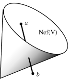
Figure 1. Irrational volume

To see this we interpret $\textnormal{vol}_{X}(L)$ as an integral. In fact, let $q(\xi)=\big{(}\xi\cdot\xi\big{)}_{V}$ be the quadratic intersection form on $N^{1}(V)_{\mathbf{R}}$, and put

$$\widehat{q}(\xi)\ =\ \begin{cases}\,q(\xi)&\text{if}\ \xi\in\textnormal{Nef}(V)\\ \,0&\text{if}\ \xi\not\in\textnormal{Nef}(V),\end{cases}$$

Then, as in [27, Section 2.3.B], one finds that

(1) $$\textnormal{vol}_{X}(L) =\ \frac{3!}{2}\cdot\int_{0}^{1}\widehat{q}\big{(}(1-t)a+tb\big{)}\,dt$$

$$=\ \frac{3!}{2}\cdot\int_{0}^{\sigma}{q}\big{(}(1-t)a+tb\big{)}\,dt,$$

where $\sigma=\sigma(a,b)$ is the largest value of $s$ such that $(1-s)a+sb$ is nef. But for general choices of $a$ and $b$, $\sigma$ is a quadratic irrationality — it arises as a root of the quadratic equation $q\big{(}(1-s)a+sb\big{)}=0$ — so the integral in (1) is typically irrational. The situation is illustrated in Figure 1. In his thesis [37], Wolfe extends this interpretation of the volume as an integral to much more general projective bundles.

We now turn to analogues of the classical properties of the volume, starting with Theorem 1.3. Let $X$ be a smooth projective variety of dimension $d$, and let $D$ be a big divisor on $X$. Take a large integer $m\gg 0$, and fix $d$ general divisors

$$E_{1},\ldots,E_{d}\ \in\ |\mspace{1.5mu}{{mD}}\mspace{1.5mu}|.$$

If $D$ fails to be ample, then it essentially never happens that the intersection of the $E_{i}$ is a finite set. Rather every divisor $E\in|\mspace{1.5mu}{{mD}}\mspace{1.5mu}|$ will contain a positive dimensional base locus $B_{m}\subseteq X$, and the $E_{i}$ will meet along $B_{m}$ as well as at a finite set of additional points. One thinks of this finite set as consisting of the “moving intersection points” of $E_{1},\ldots,E_{d}$, since (unlike $B_{m}$) they vary with the divisors $E_{i}$.

The following generalization of Theorem 1.3, which is essentially due to Fujita [18], shows that in general $\textnormal{vol}_{X}(D)$ measures the number of these moving intersection points:

Theorem 2.3 (Geometric interpretation of volume of big divisors).

Always assuming that $D$ is big, fix for $m\gg 0$ $d$ general divisors

$$E_{1}\,,\,\ldots\,,\,E_{d}\ \in\ |\mspace{1.5mu}{{mD}}\mspace{1.5mu}|$$

when $m\gg 0$, and write $B_{m}=\textnormal{Bs}\big{(}\mspace{1.1mu}|{mD}|\mspace{1.1mu}\big{)}$. Then

$$\textnormal{vol}_{X}(D)\ =\ \limsup_{m\to\infty}\frac{\#\big{(}E_{1}\,\cap\,\ldots\,\cap\,E_{d}\,\cap\,(X-B_{m})\big{)}}{m^{d}}.$$

The expression in the numerator seems to have first appeared in work of Matsusaka [29], [28], where it was called the “moving self-intersection number” of $mD$. The statement of 2.3 appears in [14], but it is implicit in Tsuji’s paper [35], and it was certainly known to Fujita as well. In fact, it is a simple consequence of Fujita’s theorem, discussed in §3, to the effect that one can approximate the volume arbitrary closely by the volume of an ample class on a modification of $X$.

Remark 2.4 (Analytic interpretation of volume).

Fujita’s theorem in turn seems to have been inspired by some remarks of Demailly in [13]. In that paper, Demailly decomposed the current corresponding to a divisor into a singular and an absolutely continuous part, and he suggested that the absolutely continuous term should correspond to the moving part of the linear series in question. Fujita seems to have been lead to his statement by the project of algebraizing Demailly’s results (see also [17] and [26, §7]). The techniques and intuition introduced by Demailly have been carried forward by Boucksom and others [3], [4], [5] in the analytic approach to asymptotic invariants.

We turn next to the variational properties of $\textnormal{vol}_{X}$. Observe to begin with that $\textnormal{vol}_{X}(D)$ is naturally defined for any $\mathbf{Q}$-divisor $D$. Indeed, one can adapt Definition 1.1 by taking the limsup over values of $m$ that are sufficiently divisible to clear the denominators of $D$. Alternatively, one can check (cf. [27, 2.2.35]) that the volume on integral divisors satisfies the homogeneity property

(2) $$\textnormal{vol}_{X}(aD)\ =\ a^{d}\cdot\textnormal{vol}_{X}(D),$$

and one can use this in turn to define $\textnormal{vol}_{X}(D)$ for $D\in\text{Div}_{\mathbf{Q}}(X)$.

The following results were proved by the second author in [27, Section 2.2.C]. They are the analogues for arbitrary big divisors of the classical Theorem 1.4.

Theorem 2.5 (Variational properties of $\textnormal{vol}_{X}$).

Let $X$ be a smooth projective variety of dimension $d$.

1. The volume of a $\mathbf{Q}$-divisor on $X$ depends only on its numerical equivalence class, and hence this invariant defines a function

   $$\textnormal{vol}_{X}\,:\,N^{1}(X)_{\mathbf{Q}}\longrightarrow\mathbf{R}.$$

2. Fix any norm $\|\ \|$ on $N^{1}(X)_{\mathbf{R}}$ inducing the usual topology on that vector space. Then there is a positive constant $C>0$ such that

   $$\big{|}\,\textnormal{vol}_{X}\big{(}\xi\big{)}\,-\,\textnormal{vol}_{X}\big{(}\xi^{\prime}\big{)}\,\big{|}\ \leq\ C\cdot\Big{(}\max\big{(}\,\|\xi\|\,,\,\|\xi^{\prime}\|\,\big{)}\Big{)}^{d-1}\cdot\|\,\xi\,-\,\xi^{\prime}\,\|$$

   for any two classes $\xi,\ \xi^{\prime}\in N^{1}(X)_{\mathbf{Q}}$.

Corollary 2.6 (Volume of real classes).

The function $\xi\mapsto\textnormal{vol}_{X}(\xi)$ on $N^{1}(X)_{\mathbf{Q}}$ extends uniquely to a continuous function

$$\textnormal{vol}_{X}\,:\,N^{1}(X)_{\mathbf{R}}\longrightarrow\mathbf{R}.\qed$$

We note that both the theorem and its corollary hold for arbitrary irreducible projective varieties. For smooth complex manifolds, the continuity of volume was established independently by Boucksom in [3]. In fact, Boucksom defines and studies the volume of an arbitrary pseudoeffective class $\alpha\in H^{{1,1}}\big{(}{X},{\mathbf{R}}\big{)}$ on a compact Kähler manifold $X$: this involves some quite sophisticated analytic methods.

One may say that the entire asymptotic Riemann–Roch problem on $X$ is encoded in the finite-dimensional vector space $N^{1}(X)_{\mathbf{R}}$ and the continuous function $\textnormal{vol}_{X}:N^{1}(X)_{\mathbf{R}}\longrightarrow\mathbf{R}$ defined on it. So it seems like a rather basic problem to understand the behavior of this invariant as closely as possible.

We next present some examples and computations.

Example 2.7 (Volume on blow-up of projective space).

The first non-trivial example is to take $X=\text{Bl}_{p}{\mathbf{P}^{d}}$ to be the blowing-up of projective space $\mathbf{P}^{d}$ at a point $p$. Write $H$ for the pull-back of a hyperplane, and $E$ for the exceptional divisor, and denote by $h,e\in N^{1}(X)_{\mathbf{R}}$ the corresponding classes. Then

$$N^{1}(X)_{\mathbf{R}}\ =\ \mathbf{R}\cdot h+\mathbf{R}\cdot e.$$

The nef cone $\textnormal{Nef}(X)$ is generated by $h-e$ and $h$, while the pseudoeffective cone is spanned by $h-e$ and $e$. On $\textnormal{Nef}(X)$, the volume is just given by the intersection form:

$$\textnormal{vol}_{X}(xh-ye)\ =\ \big{(}(xh-ye)^{d}\big{)}\ =\ x^{d}-y^{d}\ \ \ (0\leq x\leq y).$$

The sector of $N^{1}(X)$ spanned by $h$ and $e$ corresponds to linear series of the form $|\mspace{1.5mu}{{aH+bE}}\mspace{1.5mu}|$ with $b\geq 0$, and one checks that the exceptional divisor is fixed in those linear series, i.e.

$$H^{{0}}\big{(}{X},{\mathcal{O}_{X}(aH+bE)}\big{)}\ =\ H^{{0}}\big{(}{X},{\mathcal{O}_{X}(aH)}\big{)}$$

when $a,b\geq 0$. Thus if $x\geq 0\geq y$, then

$$\textnormal{vol}_{X}(xh-ye)\ =\ \textnormal{vol}_{X}(xh)\ =\ x^{d}.$$

Elsewhere the $\textnormal{vol}_{X}=0$. The situation is summarized in Figure 2, which shows $\textnormal{vol}_{X}(xh-ye)$ as a function of $(x,y)\in\mathbf{R}^{2}$.

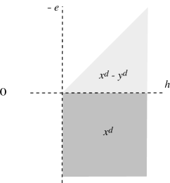
Figure 2. Volume on blow-up of $\mathbf{P}^{d}$

Example 2.8 (Toric varieties).

When $X$ is a toric variety, there is a fan refining the pseudoeffective cone of $X$, the Gel’fand-Kapranov-Zelevinski decomposition of [33], with respect to which the volume function is piecewise polynomial. In fact, recall that every torus-invariant divisor on $X$ determines a polytope $P_{D}$ such that $h^{{0}}\big{(}{X},{\mathcal{O}_{X}(D)}\big{)}$ is the number of lattice points in $P_{D}$ and $\textnormal{vol}_{X}(D)$ is the lattice volume of $P_{D}$. On the interior of each of the maximal cones in the GKZ decomposition the combinatorial type of the polytope $P_{D}$ is constant, i.e. all the polytopes have the same normal fan $\Sigma_{D}$, $D$ is the pull-back of an ample divisor $A$ on the toric variety $Y$ corresponding to $\Sigma_{D}$, and ${\rm vol}_{X}(D)={\rm vol}_{Y}(A)$.

The family of polytopes $\{P_{D}\}_{D}$ can be considered as a family of partition polytopes and the function $D\mapsto h^{{0}}\big{(}{X},{\mathcal{O}_{X}(D)}\big{)}$ is the corresponding vector partition function. Brion and Vergne [6] have studied the continuous function associated to a partition function (in our case this is precisely the volume function), and they gave explicit formulas on each of the chambers in the corresponding fan decomposition.

As we have just noted, if $X$ is a toric variety then $\textnormal{vol}_{X}$ is piecewise polynomial with respect to a polyhedral subdivision of $N^{1}(X)_{\mathbf{R}}$. This holds more generally when the linear series on $X$ satisfy a very strong hypothesis of finite generation.

Definition 2.9 (Finitely generated linear series).

We say that $X$ has finitely generated linear series if there exist integral divisors $D_{1},\ldots,D_{r}$ on $X$, whose classes form a basis of $N^{1}(X)_{\mathbf{R}}$, with the property that the $\mathbf{Z}^{r}$-graded ring

$$R\big{(}X;D_{1},\ldots,D_{r})\ =\ \bigoplus_{m_{1},\ldots m_{r}\in\mathbf{Z}}H^{{0}}\big{(}{X},{\mathcal{O}_{X}(m_{1}D_{1}+\ldots+m_{r}D_{r})}\big{)}$$

is finitely generated.

One should keep in mind that the finite generation of this ring does not in general depend only on the numerical equivalence classes of the $D_{i}$. The definition was inspired by a very closely related concept introduced and studied by Hu and Keel in [21].

Example 2.10.

It is a theorem of Cox [7] that the condition in the definition is satisfied when $X$ is a smooth toric variety, and 2.9 also holds when $X$ is a non-singular spherical variety under a reductive group. It is conjectured in [21] that smooth Fano varieties also have finitely generated linear series: this is verified by Hu and Keel in dimension three using the minimal model program.

Again inspired by the work of Hu and Keel just cited, it was established by the authors in [16] that the piecewise polynomial nature of the volume function observed in Example 2.7 holds in general on varieties with finitely generated linear series.

Theorem 2.11.

Assume that $X$ has finitely generated linear series. Then $N^{1}(X)_{\mathbf{R}}$ admits a finite polyhedral decomposition with respect to which $\textnormal{vol}_{X}$ is piecewise polynomial.

Altough the method of proof in [16] is different, in the most important cases one could deduce the theorem directly from the results of [21].

Example 2.12 (Ruled varieties over curves).

Wolfe [37] analyzed the volume function on ruled varieties over curves, and found a pleasant connection with some classical geometry. Let $C$ be a smooth projective curve of genus $g\geq 1$, and $E$ a vector bundle on $C$ of rank $e$. We consider $X=\mathbf{P}(E)$. Then

$$N^{1}(X)_{\mathbf{R}}\ =\ \mathbf{R}\cdot\xi\,+\,\mathbf{R}\cdot f,$$

where $\xi=c_{1}\big{(}\mathcal{O}_{\mathbf{P}(E)}(1)\big{)}$ is the class of the Serre line bundle and $f$ is the class of a fibre of the bundle map $\mathbf{P}(E)\longrightarrow C$. There are now two cases:

• If $E$ is semistable, then it is an old observation of Miyaoka that

  $$\textnormal{Nef}(X)\ =\ \overline{\textnormal{Eff}}(X).$$

  So in this case $\textnormal{vol}_{X}$ is just given by the intersection form on the nef cone.

• When $E$ is not semistable, it admits a canonical Harder-Narasimhan filtration with semistable graded pieces. Wolfe shows that this determines a decomposition of $\overline{\textnormal{Eff}}(X)$ into finitely many sectors — one for each piece of the filtration — on which $\textnormal{vol}_{X}$ is given by a polynomial.

The situation is illustrated in Figure 3. In summary we may say that the basic geometry associated to the vector bundle $E$ is visible in the volume function on $X=\mathbf{P}(E)$.

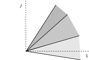
Figure 3. Volume on projective bundle over curve

Problem 2.13.

It would be worthwhile to work out examples of the volume function $\textnormal{vol}_{X}$ when $X$ is the projectivization of a bundle $E$ on a higher dimensional base. Here one might expect more complicated behavior, and it would be interesting to see to what extent the geometry of $E$ is reflected in $\textnormal{vol}_{X}$.

In the case of surfaces, the volume function was analyzed by Bauer, Küronya and Szemberg in [2], who prove:

Theorem 2.14 (Volume function on surfaces).

Let $X$ be a smooth surface. Then $\textnormal{Big}(X)$ admits a locally finite rational polyhedral subdivision on which $\textnormal{vol}_{X}$ is piecewise polynomial.

The essential point here is that on surfaces, the volume of a big divisor $D$ is governed by the Zariski decomposition of $D$, which gives a canonical expression $D=P+N$ of the divisor in question as the sum of a “positive” and “negative part” (see for instance [1], or [2]). It is immediate that $\textnormal{vol}_{X}(D)=\big{(}P^{2}\big{)}_{X}$, so the issue is to understand how this decomposition varies with $D$.

On the other hand, in the same paper [2], Bauer, Küronya and Szemberg give examples to prove:

Proposition 2.15.

There exists a smooth projective threefold $X$ for which

$$\textnormal{vol}_{X}:N^{1}(X)_{\mathbf{R}}\longrightarrow\mathbf{R}$$

is piecewise analytic but not piecewise polynomial.

This shows that in general, the volume function has a fundamentally non-classical nature.

Example 2.16 (Threefold with non-polynomial volume).

The idea of [2] is to study the volume function on the threefold $X$ constructed in Example 2.7. Keeping the notation of that example, fix a divisor $C$ on $V$ with class $c\in N^{1}(X)_{\mathbf{R}}$. In view of the homogeneity (2) of volume, the essential point is to understand how the volume of the line bundle

$$L_{C}\ =_{\text{def}}\ \mathcal{O}_{\mathbf{P}}(1)\otimes\pi^{*}\mathcal{O}_{V}(C)$$

varies with $C$, where $\pi:X=\mathbf{P}\big{(}\mathcal{O}_{V}(A)\oplus\mathcal{O}_{V}(B)\big{)}\longrightarrow V$ is the bundle map. For this one can proceed as in Example 2.7. One finds that

$$\textnormal{vol}_{X}(L_{C})\ =\ \frac{3!}{2}\cdot\int_{0}^{\sigma(c)}{q}\big{(}c+(1-t)a+tb\big{)}\,dt,$$

where $\sigma(c)$ denotes the largest value of $s$ for which $(1-s)a+sb+c$ is nef. On the other hand, if $c$ is small enough so that $a+c$ is nef while $b+c$ is not, then $\sigma(c)$ is not given by a polynomial in $c$ (although $\sigma(c)$ is an algebraic function of $c$). So one does not expect — and it is not the case — that $\textnormal{vol}_{X}(L_{C})$ varies polynomially with $C$.

Returning to the case of a smooth projective variety $X$ of arbitrary dimension $d$, the second author observed in [27, Theorem 11.4.9] that Theorem 1.5 extends to arbitrary big divisors:

Theorem 2.17 (Log-concavity of volume).

The inequality

$$\textnormal{vol}_{X}(\xi+\xi^{\prime})^{1/d}\ \geq\ \textnormal{vol}_{X}(\xi)^{1/d}\,+\,\textnormal{vol}_{X}(\xi^{\prime})^{1/d}.$$

holds for any two classes $\xi,\xi^{\prime}\in\textnormal{Big}(X)$.

Although seemingly somewhat delicate, this actually follows immediately from the theorem of Fujita that we discuss in the next section.

As of this writing, Theorems 2.5 and 2.17 represent the only regularity properties that the volume function $\textnormal{vol}_{X}$ is known to satisfy in general. It would be very interesting to know whether in fact there are others. The natural expectation is that $\textnormal{vol}_{X}$ is “typically” real analytic:

Conjecture 2.18.

There is a “large” open set $U\subseteq\textnormal{Big}(X)$ such that $\textnormal{vol}_{X}$ is real analytic on each connected component of $U$.

One could hope more precisely that $U$ is actually dense, but this might run into trouble with clustering phenomena. We refer to Section 6 for a description of some “laboratory experiments” that have been performed on a related invariant.

3. Fujita’s Approximation Theorem

One of the most important facts about $\textnormal{vol}_{X}$ — and the source of several of the results stated in the previous section — is a theorem of Fujita [18] to the effect that one can approximate the volume of an arbitrary big divisor by the top-self intersection number of an ample line bundle on a blow-up of the variety in question. We briefly discuss Fujita’s result here.

As before, let $X$ be a smooth projective variety and consider a big class $\xi\in N^{1}(X)_{\mathbf{R}}$. As a matter of terminology, we declare that a Fujita approximation of $\xi$ consists of a birational morphism

$$\mu:X^{\prime}\longrightarrow X,$$

from a smooth projective variety $X^{\prime}$ onto $X$, together with a decomposition

$$\mu^{*}\xi\ =\ a\,+\,e\ \in\ N^{1}(X^{\prime})_{\mathbf{R}},$$

where $a$ is an ample class and $e$ is an effective class on $X^{\prime}$.

Fujita’s theorem asserts that one can find such an approximation in which the volume of $a$ approximates arbitrarily closely the volume of $\xi$:

Theorem 3.1 (Fujita’s approximation theorem).

Given any $\varepsilon>0$, there exists a Fujita approximation

$$\mu:X^{\prime}\longrightarrow X\ \ ,\ \ \mu^{*}(\xi)\ =\ a\,+\,e$$

where $|\textnormal{vol}_{X}(\xi)-\textnormal{vol}_{X^{\prime}}(a)|<\varepsilon$.

We stress that the output of the theorem depends on $\varepsilon$. We note that Theorems 2.3 and 2.17 follow almost immediately from this result.

For the proof, one reduces by continuity and homogeneity to the situation when $\xi$ represents an integer divisor $D$. Given $m\gg 0$, denote by $\mathfrak{b}_{m}\subseteq\mathcal{O}_{X}$ the base-ideal of $|\mspace{1.5mu}{{mD}}\mspace{1.5mu}|$, and let $\mu_{m}:X_{m}\longrightarrow X$ be a resolution of singularities of the blowing-up of $\mathfrak{b}_{m}$. Then on $X_{m}$ one can write

$$\mu_{m}^{*}(mD)\ =\ B_{m}\,+\,E_{m},$$

where $B_{m}$ is free and $E_{m}$ is (the pullback of) the exceptional divisor of the blow-up. The strategy is to take $A_{m}=\tfrac{1}{m}B_{m}$ as the positive part of the approximation. It is automatic that $\textnormal{vol}_{X_{m}}(A_{m})\leq\textnormal{vol}_{X}(D)$, so the essential point is to prove that

$$\textnormal{vol}_{X_{m}}(A_{m})\ >\ \textnormal{vol}_{X}(D)\,-\,\varepsilon$$

provided that $m$ is sufficiently large (with the bound depending on $\varepsilon$). Fujita’s original proof was elementary but quite tricky; a more conceptual proof using multiplier ideals appears in [14], and yet another argument, revolving around higher jets, is given in [31].

Boucksom, Demailly, Paun and Peternell established in [5] an important “orthogonality” property of Fujita approximations. Specifically, they prove:

Theorem 3.2.

In the situation of Theorem 3.1, fix an ample class $h$ on $X$ which is sufficiently positive so that $h\pm\xi$ is ample. Then there is a universal constant $C$ such that

$$\big{(}a^{n-1}\cdot e\big{)}^{2}_{X^{\prime}}\ \leq\ C\cdot\big{(}h^{n}\big{)}_{X}\cdot\big{(}\textnormal{vol}_{X}(\xi)\,-\,\textnormal{vol}_{X^{\prime}}(a)\big{)}.$$

In other words, as one passes to a better and better Fujita approximation, the exceptional divisor of the approximation becomes more nearly orthogonal to the ample part of $\xi$. This had been conjectured by the fourth author in [31]. Boucksom–Demailly–Paun–Peternell use this to identify the cone of curves dual to the pseudoeffective cone. Accounts of this work appears in [12] and in [27, §11.4.C].

4. Higher Cohomology

The volume $\textnormal{vol}_{X}(D)$ measures the asymptotic behavior of the dimension $h^{0}\big{(}mD\big{)}$. But of course it has been well-understood since Serre that one should also consider higher cohomology groups. We discuss in this section invariants involving the groups $H^{{i}}\big{(}{X},{\mathcal{O}_{X}(mD)}\big{)}$ for $i\geq 1$.

As always, $X$ denotes a smooth projective variety of dimension $d$, and $D$ is a divisor on $X$.

Definition 4.1 (Asymptotic cohomology function).

Given $i\geq 0$, the $i^{\text{th}}$ asymptotic cohomology function associated to $D$ is

$$\widehat{h}^{{i}}\big{(}{D}\big{)}\ =\ \limsup\,\frac{h^{{i}}\big{(}{X},{\mathcal{O}_{X}(mD)}\big{)}}{m^{d}/d!}.$$

Thus $\textnormal{vol}_{X}(D)=\widehat{h}^{{0}}\big{(}{D}\big{)}$. By working with sufficiently divisible $m$, or establishing the homogeneity of $\widehat{h}^{i}$ as in equation (2), the definition extends in a natural way to $\mathbf{Q}$-divisors. However we remark that it is not known that the limsup in the definition is actually a limit, although one hopes that this is the case.

These higher cohomology functions were studied in [25] by Küronya, who establishes for them the analogue of Theorem 2.5:

Theorem 4.2.

The function $\widehat{h}^{{i}}\big{(}{D}\big{)}$ depends only on the numerical equivalence class of a $\mathbf{Q}$-divisor $D$, and it extends uniquely to a continuous function

$$\widehat{h}^{i}:N^{1}(X)_{\mathbf{R}}\longrightarrow\mathbf{R}.$$

Note that in contrast to the volume, these functions can be non-vanishing away from the big cone. For example, it follows from Serre duality that the highest function $\widehat{h}^{d}$ is supported on $-\overline{\textnormal{Eff}}(X)$.

Example 4.3 (Blow-up of $\mathbf{P}^{d}$).

Returning to the situation of Example 2.7, let $X=\text{Bl}_{p}(\mathbf{P}^{d})$ be the blowing up of projective space at a point, and consider the region $x>0>y$ of $N^{1}(X)_{\mathbf{R}}=\mathbf{R}^{2}$ where the class $xh-ye$ is big but not ample. In this sector, $\widehat{h}^{i}=0$ unless $i=0$ or $i=d-1$, and

$$\widehat{h}^{0}\big{(}xh-ye\big{)}=x^{d}\ \ \ ,\ \ \ \ \widehat{h}^{d-1}\big{(}xh-ye\big{)}\ =\ (-1)^{d}\cdot y^{d}.$$

Example 4.4 (Abelian varieties, [25], §3.1).

Let $X$ be an abelian variety of dimension $d$. Here the higher cohomology functions reflect the classical theory of indices of line bundles on abelian varieties. Specifically, express $X$ as the quotient $X=V/\Lambda$ of a $d$-dimensional complex vector space $V$ by a lattice $\Lambda\subseteq V$. Then $H^{{1,1}}\big{(}{X},{\mathbf{R}}\big{)}$ is identified with the real vector space of hermitian forms on $V$, and $N^{1}(X)_{\mathbf{R}}\subseteq H^{{1,1}}\big{(}{X},{\mathbf{R}}\big{)}$ is the subspace spanned by those forms whose imaginary part takes integer values on $\Lambda$. The dense open subset of this Néron–Severi space corresponding to non-degenerate forms is partitioned into disjoint open cones

$$\textnormal{Ind}_{j}(X)\ \subseteq\ N^{1}(X)_{\mathbf{R}}$$

according to the index (i.e. the number of negative eigenvalues) of the form in question. Then given $\xi\in N^{1}(X)_{\mathbf{R}}$, one has

$$\widehat{h}^{{i}}\big{(}{\xi}\big{)}\ =\ \begin{cases}(-1)^{i}\cdot\int_{X}\xi^{d}&\text{ if }\,\xi\,\in\,\textnormal{Ind}_{i}(X)\\ 0&\text{ if }\,\xi\,\not\in\,\textnormal{Ind}_{i}(X).\end{cases}$$

For instance, suppose that $X$ has dimension $2$ and Picard number $\rho(X)=3$. Then (as in Example 2.2) the cone of classes having self-intersection $=0$ divides $N^{1}(X)_{\mathbf{R}}$ into three regions. The classes with $\widehat{h}^{0}\neq 0$ and $\widehat{h}^{2}\neq 0$ occupy the two conical regions, while the exterior of the cone consists of classes with $\widehat{h}^{1}\neq 0$. The situation is illustrated in Figure 4.

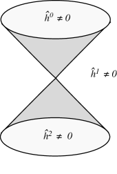
Figure 4. Higher cohomology on abelian surface

Example 4.5 (Flag varieties).

Let $X=G/B$ be the quotient of a semi-simple algebraic group by a Borel subgroup. Then the Borel–Bott–Weil theorem gives a finite decomposition of $N^{1}(X)_{\mathbf{R}}$ into polyhedral chambers on which exactly one of the functions $\widehat{h}^{i}$ is non-zero. See [25, §3.3] for details.

Remark 4.6 (Toric varieties).

When $X$ is a projective toric variety, the functions $\widehat{h}^{i}$ are studied by Hering, Küronya and Payne in [20]. In this case, the functions are again piecewise polynomial on a polyhedral decomposition of $N^{1}(X)_{\mathbf{R}}$, although in general one needs to refine the GKZ-decomposition with respect to which $\textnormal{vol}_{X}$ is piecewise polynomial.

It is interesting to ask what geometric information these functions convey. De Fernex, Küronya and the second author [11] have established that ample classes are characterized by vanishings involving the higher cohomology functions.

Theorem 4.7 (Characterization of ample classes).

Let

$$\xi_{0}\ \in\ N^{1}(X)_{\mathbf{R}}$$

be any class. Then $\xi_{0}$ is ample if and only if there exists a neighborhood $U\subseteq N^{1}(X)_{\mathbf{R}}$ of $\xi_{0}$ such that

$$\widehat{h}^{i}(\xi)\ =\ 0$$

for all $i>0$ and every $\xi\in U$.

As one sees for instance from Example 4.4, it can happen that $\widehat{h}^{i}(\xi_{0})=0$ for all $i$ without $\xi_{0}$ being ample (or even pseudoeffective), so one can’t avoid looking at a neighborhood of $\xi_{0}$. One can view Theorem 4.7 as an asymptotic analogue of Serre’s criterion for amplitude. The essential content of the result is that if $D$ is a big divisor that is not nef, and if $A$ is any ample divisor, then $\widehat{h}^{{i}}\big{(}{D-tA}\big{)}\neq 0$ for some $i>0$ and sufficiently small $t>0$.

5. Base Loci

Big divisors that fail to be nef are essentially characterized by the asymptotic presence of base-loci. It is then natural to try to measure quantitatively the loci in question. This was first undertaken by Nakayama [32], and developed from another viewpoint in the paper [16] of the present authors. Nakayama’s results were generalized and extended to the analytic setting by Boucksom in [4].

As before, let $X$ be a smooth projective variety of dimension $d$. Denote by $\textnormal{ord}_{E}$ a divisorial valuation centered on $X$. Concretely, this is given by a projective birational morphism $\mu:X^{\prime}\longrightarrow X$, say with $X^{\prime}$ smooth, together with an irreducible divisor $E\subseteq X^{\prime}$. Given locally a regular function $f$ on $X$, one can then discuss the order

$$\textnormal{ord}_{E}(f)\ \in\ \mathbf{N}$$

of vanishing of $f$ along $E$. For an effective divisor $D$ on $X$, the order $\textnormal{ord}_{E}(D)$ of $D$ along $E$ is defined via a local equation for $D$.

Example 5.1 (Order of vanishing at a point or along a subvariety).

Fix a point $x\in X$, and let $E$ denote the exceptional divisor in the blow-up $\text{Bl}_{x}(X)$. Then $\textnormal{ord}_{E}=\textnormal{ord}_{x}$ is just the classical order of vanishing at $x$: one has

$$\textnormal{ord}_{x}(f)\ =\ a$$

if and only if all partials of $f$ of order $<a$ vanish at $x$, while some $a^{\text{th}}$ partial is $\neq 0$. Given any proper irreducible subvariety $Z\subseteq X$, the order of vanishing $\textnormal{ord}_{Z}$ is defined similarly.

Now let $D$ be a big divisor on $X$. Then one sets

$$\textnormal{ord}_{E}\big{(}|\mspace{1.5mu}{{D}}\mspace{1.5mu}|\big{)}\ =\ \min_{D^{\prime}\in|\mspace{1.5mu}{{D}}\mspace{1.5mu}|}\textnormal{ord}_{E}\big{(}D^{\prime}\big{)}$$

$$\textnormal{ord}_{E}\big{(}\|\mspace{1.5mu}{D}\mspace{1.5mu}\|\big{)}\ =\ \limsup\frac{\textnormal{ord}_{E}\big{(}|\mspace{1.5mu}{{mD}}\mspace{1.5mu}|\big{)}}{m}.$$

These definitions once again extend in a natural way to $\mathbf{Q}$-divisors, and then one has:

Theorem 5.2.

The function $\textnormal{ord}_{E}\big{(}\|\mspace{1.5mu}{D}\mspace{1.5mu}\|\big{)}$ depends only on the numerical equivalence class of a big $\mathbf{Q}$-divisor $D$, and it extends to a continuous function

(3) $$\textnormal{ord}_{E}\,:\,\textnormal{Big}(X)\longrightarrow\mathbf{R}.$$

This was initially established by Nakayama for order of vanishing along a subvariety, and extended to more general valuations in [16].

The paper [16] also analyzes precisely when this invariant vanishes. Recall for this that the stable base-locus $\mathbf{B}({D})$ of a big divisor (or $\mathbf{Q}$-divisor) $D$ is defined to be the common base-locus of the linear series $|\mspace{1.5mu}{{mD}}\mspace{1.5mu}|$ for sufficiently large and divisible $m$. (See [27, Section 2.1.A] for details.)

Theorem 5.3.

Keeping notation as above, let $Z$ be the center of $E$ on $X$. If $D$ is a big divisor on $X$, then

$$\textnormal{ord}_{E}\big{(}\|\mspace{1.5mu}{D}\mspace{1.5mu}\|\big{)}\ >\ 0$$

if and only if there exists an ample $\mathbf{Q}$-divisor $A$ such that $Z$ is contained in the stable base-locus $\mathbf{B}({D+A})$ of $D+A$.

One thinks of $D+A$ as a small positive perturbation of $D$. The union of the sets $\mathbf{B}({D+A})$ is called in [5] the non-nef locus of $D$. With a little more care about the definitions, one can prove the analogous statement with $D$ replaced by an arbitrary big class $\xi\in\text{Big}(X)$.

Building on ideas first introduced by the fourth author in [30] and [31], one can also use a volume-like invariant to analyze what subvarieties appear as irreducible components of the stable base-locus. In fact, let $Z\subseteq X$ be an irreducible subvariety of dimension $e$, and let $D$ be a big divisor on $X$. Set

$$V_{m}\ =\ \text{Image}\Big{(}H^{{0}}\big{(}{X},{\mathcal{O}_{X}(mD)}\big{)}\longrightarrow H^{{0}}\big{(}{Z},{\mathcal{O}_{Z}(mD)}\big{)}\Big{)}.$$

Thus $V_{m}$ is a (possibly proper) subspace of the space of sections of $\mathcal{O}_{Z}(mD)$. We define the restricted volume of $D$ to $Z$ to be

$$\textnormal{vol}_{X|Z}(D)\ =\ \limsup\frac{\dim V_{m}}{m^{e}/e!}.$$

For instance if $D$ is ample then the restriction mappings are eventually surjective, and hence

$$\textnormal{vol}_{X|Z}(D)\ =\ \textnormal{vol}_{Z}(D|Z)\ =\ \big{(}D^{e}\cdot Z\big{)}.$$

However in general it can happen that $\textnormal{vol}_{X|Z}(D)<\textnormal{vol}_{Z}(D|Z)$. An analogue of Theorem 2.3 holds for these restricted volumes. Again the definition extends naturally to $\mathbf{Q}$-divisors $D$ (and $\mathbf{R}$-divisors as well).

Given any $\mathbf{Q}$-divisor $D$, the augmented base-locus of $D$ is defined to be

$$\mathbf{B}_{+}({D})\ =\ \mathbf{B}({D-A})$$

for any ample $\mathbf{Q}$-divisor $A$ whose class in $N^{1}(X)_{\mathbf{R}}$ is sufficiently small (this being independent of the particular choice of $A$). It was discovered by the fourth author in [30] that this augmented base-locus behaves more predictably that $\mathbf{B}({D})$ itself. (See [27, Chapter 10.4] for an account.)

Building on the ideas and techniques of [31], the authors prove in [15]

Theorem 5.4.

Let $D$ be a big $\mathbf{Q}$-divisor on $X$, and let $Z\subseteq X$ be a subvariety. If $Z$ is an irreducible component of $\mathbf{B}_{+}({D})$, then

$$\lim_{D^{\prime}\longrightarrow D}\textnormal{vol}_{X|Z}(D^{\prime})\ =\ 0,$$

the limit being taken over all big $\mathbf{Q}$-divisors approaching $D$. Conversely, if $Z\not\subseteq\mathbf{B}_{+}({D})$, then

$$\lim_{D^{\prime}\longrightarrow D}\textnormal{vol}_{X|Z}(D^{\prime})\ =\ \textnormal{vol}_{X|Z}(D)\ >\ 0.$$

We remark that the statement remains true also when $D$ is an $\mathbf{R}$-divisor.

6. In Vitro Linear Series

Just as it is interesting to ask about the regularity of the volume function, it is also natural to inquire about the nature of the order function occuring in (3). To shed light on this question, one can consider an abstract algebraic construction that models some of the global behavior that can occur for global linear series.

Let $X$ be a smooth projective variety of dimension $d$. The starting point is the observation that the pseudoeffective and nef cones

$$\textnormal{Nef}(X)\ \subseteq\ \overline{\textnormal{Eff}}(X)\ \subseteq\ N^{1}(X)_{\mathbf{R}}$$

on $X$, as well as the order function in (3), can be recovered formally from the base-ideals of linear series on $X$. Specifically, fix integer divisors $D_{1},\ldots,D_{r}$ on $X$ whose classes form a basis of $N^{1}(X)_{\mathbf{R}}$: note that this determines an identification $N^{1}(X)_{\mathbf{R}}=\mathbf{R}^{r}$. Given inegers $m_{1},\ldots,m_{r}\in\mathbf{Z}$, write $\vec{m}=(m_{1},\ldots,m_{r})$, and let

$$\mathfrak{b}_{\vec{m}}\ =\ \mathfrak{b}\big{(}\mspace{1.1mu}|\mspace{1.5mu}{{{m_{1}D_{1}+\ldots+m_{r}D_{r}}}}\mspace{1.5mu}|\mspace{1.1mu}\big{)}$$

be the base ideal of the corresponding linear series. Thus $\mathfrak{b}_{\vec{m}}\subseteq\mathcal{O}_{X}$ is an ideal sheaf on $X$, and one has

(4) $$\mathfrak{b}_{\vec{m}}\cdot\mathfrak{b}_{\vec{\ell}}\ \subseteq\ \mathfrak{b}_{\vec{m}+\vec{\ell}}$$

for every $\vec{m},\vec{\ell}\in\mathbf{Z}^{r}$. Note that we can recover the nef and pseudoeffective cones on $X$ from these ideals. In fact, a moment’s thought shows that $\textnormal{Nef}(X)\subseteq\mathbf{R}^{r}$ is the closed convex cone spanned by all vectors $\vec{m}\in\mathbf{Z}^{r}$ such that $\mathfrak{b}_{\vec{m}}=\mathcal{O}_{X}$, and similarly $\overline{\textnormal{Eff}}(X)$ is the closed convex cone generated by all $\vec{m}$ such that $\mathfrak{b}_{\vec{m}}\neq(0)$. The function

$$\textnormal{ord}_{Z}\,:\,\textnormal{Big}(X)_{\mathbf{R}}\longrightarrow\mathbf{R}$$

measuring order of vanishing along a subvariety $Z\subseteq X$ discussed in the previous section can also be defined just using these ideals.

This leads one to consider arbitrary collections of ideal sheaves satisfying the basic multiplicativity property (4): they provide abstract models of linear series. Specifically, let $V$ be any smooth variety of dimension $d$ (for example $V=\mathbf{C}^{d})$. A multi-graded family of ideals on $V$ is a collection

$$\mathfrak{a}_{\bullet}\ =\ \big{\{}\mathfrak{a}_{\vec{m}}\big{\}}_{\vec{m}\in\mathbf{Z}^{m}}$$

of ideal sheaves $\mathfrak{a}_{\vec{m}}\subseteq\mathcal{O}_{V}$ on $V$, indexed by $\mathbf{Z}^{r}$, such that $\mathfrak{a}_{\vec{0}}=\mathcal{O}_{V}$, and

$$\mathfrak{a}_{\vec{m}}\cdot\mathfrak{a}_{\vec{\ell}}\ \subseteq\ \mathfrak{a}_{\vec{m}+\vec{\ell}}$$

for all $\vec{m},\vec{\ell}\in\mathbf{Z}^{r}$. One puts $N^{1}(\mathfrak{a}_{\bullet})_{\mathbf{R}}=\mathbf{Z}^{r}\otimes_{\mathbf{Z}}\mathbf{R}=\mathbf{R}^{r}$, and

$$\textnormal{Nef}(\mathfrak{a}_{\bullet})\ \subseteq\ \overline{\textnormal{Eff}}(\mathfrak{a}_{\bullet})\ \subseteq\ N^{1}(\mathfrak{a}_{\bullet})_{\mathbf{R}}$$

are defined as above. Then $\text{Amp}(\mathfrak{a}_{\bullet})$ and $\text{Big}(\mathfrak{a}_{\bullet})$ are taken to be the interiors of these cones.

Now fix a subvariety $Z\subseteq V$. Then under mild assumptions on $\mathfrak{a}_{\bullet}$, one can mimic the global constructions to define a continuous function

$$\textnormal{ord}_{Z}:\text{Big}(\mathfrak{a}_{\bullet})\longrightarrow\mathbf{R}$$

that coincides with the global function when $\mathfrak{a}_{\bullet}$ is the system of base-ideals just discussed. We refer to [16], [36] and [37] for details.

The interesting point is that in this abstract setting, the function $\textnormal{ord}_{Z}$ can be wild. In fact, Wolfe [36] proves:

Theorem 6.1.

There exist multi-graded families $\{\mathfrak{a}_{\bullet}\}$ of monomial ideals on $V=\mathbf{C}^{n}$ for which the function

$$\textnormal{ord}_{0}:\textnormal{Big}(\mathfrak{a}_{\bullet})\longrightarrow\mathbf{R}$$

is nowhere differentiable on an open set.

One conjectures of course that this sort of behavior cannot occur in the global setting. However all the known properties of $\textnormal{ord}_{E}$ can be established in this formal setting. So one is led to expect that there should be global properties of these invariants that have yet to be discovered.

References

- [1] Lucian Bădescu, Algebraic Surfaces, Universitext, Springer-Verlag, New York, 2001.
- [2] Thomas Bauer, Alex Küronya, and Tomasz Szemberg, Zariski chambers, volumes, and stable base loci, J. Reine Angew. Math. 576 (2004), 209–233.
- [3] Sébastien Boucksom, On the volume of a line bundle, Internat. J. Math. 13 (2002), no. 10, 1043–1063.
- [4] Sébastien Boucksom, Divisorial Zariski decompositions on compact complex manifolds, Ann. Sci. École Norm. Sup. (4) 37 (2004), no. 1, 45–76.
- [5] Sébastien Boucksom, Jean-Pierre Demailly, Mihai Paun, and Thomas Peternell, The pseudo-effective cone of a compact Kähler manifold and varieties of negative Kodaira dimension, preprint, 2004.
- [6] Michel Brion and Michèle Vergne, Residue formulae, vector partition functions and lattice points in rational polytopes, J. Amer. Math. Soc. 10 (1997), no. 4, 797–833.
- [7] David A. Cox, The homogeneous coordinate ring of a toric variety, J. Algebraic Geom. 4 (1995), no. 1, 17–50.
- [8] S. Dale Cutkosky, Zariski decomposition of divisors on algebraic varieties, Duke Math. J. 53 (1986), no. 1, 149–156.
- [9] S. Dale Cutkosky and V. Srinivas, On a problem of Zariski on dimensions of linear systems, Ann. of Math. (2) 137 (1993), no. 3, 531–559.
- [10] by same author, Periodicity of the fixed locus of multiples of a divisor on a surface, Duke Math. J. 72 (1993), no. 3, 641–647.
- [11] Tommaso De Fernex, Alex Küronya, and Robert Lazarsfeld, Higher cohomology of big divisors, in preparation.
- [12] Olivier Debarre, Classes de cohomologie positives dans les variétés kählériennes compactes, Seminaire Bourbaki, Exposé 943, 2005.
- [13] Jean-Pierre Demailly, A numerical criterion for very ample line bundles, J. Differential Geom. 37 (1993), no. 2, 323–374.
- [14] Jean-Pierre Demailly, Lawrence Ein, and Robert Lazarsfeld, A subadditivity property of multiplier ideals, Michigan Math. J. 48 (2000), 137–156.
- [15] Lawrence Ein, Robert Lazarsfeld, Mircea Mustaţǎ, Michael Nakamaye, and Mihnea Popa, Restricted volumes and asymptotic intersection theory, in preparation.
- [16] by same author, Asymptotic invariants of base loci, preprint, 2003.
- [17] Lawrence Ein, Robert Lazarsfeld, and Michael Nakamaye, Zero-estimates, intersection theory, and a theorem of Demailly, Higher-Dimensional Complex Varieties (Trento, 1994), de Gruyter, Berlin, 1996, pp. 183–207.
- [18] Takao Fujita, Approximating Zariski decomposition of big line bundles, Kodai Math. J. 17 (1994), no. 1, 1–3.
- [19] Mikhael Gromov, Convex sets and Kähler manifolds, Advances in Differential Geometry and Topology, World Sci. Publishing, Teaneck, NJ, 1990, pp. 1–38.
- [20] Milena Hering, Alex Küronya, and Sam Payne, Asymptotic cohomological functions of toric divisors, preprint, 2005.
- [21] Yi Hu and Sean Keel, Mori dream spaces and GIT, Michigan Math. J. 48 (2000), 331–348.
- [22] Daniel Huybrechts and Manfred Lehn, The Geometry of Moduli Spaces of Sheaves, Aspects of Mathematics, E31, Friedr. Vieweg & Sohn, Braunschweig, 1997.
- [23] Friedrich Knop, Über Hilberts vierzehntes Problem für Varietäten mit Kompliziertheit eins, Math. Z. 213 (1993), no. 1, 33–36.
- [24] János Kollár and T. Matsusaka, Riemann–Roch type inequalities, Amer. J. Math. 105 (1983), no. 1, 229–252.
- [25] Alex Küronya, Asymptotic cohomological functions on projective varieties, preprint, 2005.
- [26] Robert Lazarsfeld, Lectures on linear series, Complex Algebraic Geometry (Park City, UT, 1993), IAS/Park City Math. Series, vol. 3, Amer. Math. Soc., Providence, RI, 1997, pp. 161–219.
- [27] by same author, Positivity in Algebraic Geometry. I & II, Ergebnisse der Mathematik und ihrer Grenzgebiete., vol. 48 & 49, Springer-Verlag, Berlin, 2004.
- [28] David Lieberman and David Mumford, Matsusaka’s big theorem, Algebraic Geometry – Arcata 1974, Proc. Symp. Pure Math., vol. 29, Amer. Math. Soc., 1975, pp. 513–530.
- [29] T. Matsusaka, Polarized varieties with a given Hilbert polynomial, Amer. J. Math. 94 (1972), 1027–1077.
- [30] Michael Nakamaye, Stable base loci of linear series, Math. Ann. 318 (2000), no. 4, 837–847.
- [31] by same author, Base loci of linear series are numerically determined, Trans. Amer. Math. Soc. 355 (2003), no. 2, 551–566.
- [32] Noboru Nakayama, Zariski-decomposition and abundance, MSJ Memoirs, vol. 14, Mathematical Society of Japan, Tokyo, 2004.
- [33] Tadao Oda and Hye Sook Park, Linear Gale transforms and Gel′fand-Kapranov-Zelevinskij decompositions, Tohoku Math. J. (2) 43 (1991), no. 3, 375–399.
- [34] Andrei Okounkov, Why would multiplicities be log-concave?, The orbit method in geometry and physics (Marseille, 2000), Progr. Math., vol. 213, Birkhäuser Boston, Boston, MA, 2003, pp. 329–347.
- [35] Hajime Tsuji, On the structure of pluricanonical systems of projective varieties of general type, preprint, 1999.
- [36] Alexandre Wolfe, Cones and asymptotic invariants of multigraded systems of ideals, preprint, 2003.
- [37] by same author, Asymptotic invariants of graded systems of ideals and linear systems on projective bundles, Ph.D. thesis, University of Michigan, 2005.
- [38] Oscar Zariski, The theorem of Riemann–Roch for high multiples of an effective divisor on an algebraic surface, Ann. of Math. (2) 76 (1962), 560–615.