The stability of join-the-shortest-queue models with general input and output processes

Abstract.

The paper establishes necessary and sufficient conditions for stability of different join-the-shortest-queue models including load-balanced networks with general input and output processes. It is shown, that the necessary and sufficient condition for stability of load-balanced networks is associated with the solution of a linear programming problem precisely formulated in the paper. It is proved, that if the minimum of the objective function of that linear programming problem is less than 1, then the associated load-balanced network is stable.

1. Introduction

1.1. The goal of the paper

The theory of parallel queues is a distinguished area of queueing theory. Parallel queues have good properties (e.g. Halfin [28], Mitzenmacher [43], Winston [55]) resulting in various applications in different areas of science and technology. The literature on parallel queues is very rich and includes solutions of a large number of various theoretical and applied problems. In this context we mention the pioneering paper of Flatto and McKean [20], the papers of Flatto [18], Flatto and Hahn [19], as well as the recent paper of Kurkova and Suhov [34] for mentioning a few.

During the last years there has been increasing interest in parallel queueing systems due to a growing development of telecommunication technologies. As a result, there has been substantially increasing number of related publications including such areas as routing and admission control problems, scheduling and many other areas using the join-the-shortest-queue (JS-queue) policy.

Despite of many existing publications on JS-queue models, it is still not a well-studied area. There is a large number of unsolved problems or problems the solution of which is very far from its completion. One of them is a problem of stability. The stability (instability) of different JS-queue (together with stability other closely related models) has been studied in many papers. We refer to the papers of Foley and McDonald [21], Foss and Chernova [22], [23], Kurkova [33], Sharifnia [48], Suhov and Vvedenskaya [51], Tandra, Hemachandra and Manjunath [52], Vvedenskaya and Suhov [54], and Vvedenskaya, Dobrushin and Karpelevich [53]. Particularly, the stability of a Markovian load-balanced network, consisting of two stations only, has been studied in [33].

In the present paper, we establish necessary and sufficient conditions of stability for a wide class of load-balanced networks, the arrival and departure processes of which are assumed to be quite general. The exact description of these processes will be provided later in the paper.

1.2. Motivation

The stability of stochastic processes and especially queueing systems and networks of queues is a very significant area of research. The first results on the stability of queues go back to the well-known pioneering papers of Lindley [35] and Kiefer and Wolfowitz [31] on the stability of classic single-server and multiserver queueing systems. One of the most significant contribution to stability of queueing systems was made slightly later by Loynes [36], who was the first person to establish the stability of single-server queues with dependent interarrival and service times. The approach of Loynes [36] is well-known and has been widely used to prove the stability of various queueing systems. It led to a new vision of the stability for models with dependent interarrival and/or service times, and has been a source for new methods of the stability of complex queueing models. Among them there are renovative theory and recurrence equation methods (e.g. [5], [6], [7], [8], [11], [14], [15], [24] and many others) as well as a martingale-based approach of [3].

However, the development of the Loynes approach towards queueing networks, because of their complicated nature, has been problematical, and the proof of the stability and ergodicity of queueing networks is typically based on other methods based on the special theories of Markov and regeneration processes.

The first results on the stability of Jackson-type queueing networks have been obtained by Borovkov [12], [13]. Then the stability and ergodicity of networks have been studied in many papers. We mention the papers related to the stability of Jackson-type networks by Meyn and Down [38], Kaspi and Mandelbaum [29], [30], Sigman [49] and Baccelli and Foss [9]. All of these papers, but [9], are based on regeneration phenomena of the theory of Harris recurrent Markov chains.

The theory of Harris recurrent Markov chains had been exposed in the books of Orey [44] and Revuz [46]. The detailed study of stochastic stability of Markov chains and the theory of Harris recurrent Markov processes can be found in the book of Meyn and Tweedie [42], and in a number of research papers of these authors [39], [40] and [41].

However, the proof of networks stability by the means of Harris recurrent Markov chains is restrictive. Being very difficult technically, it works in the cases where the sequences of interarrival and service times consist of independent random variables. In this case the phase space of the process can be expanded to Markov, and a network stability is proved in terms of the stability of the corresponding Markov process. As a rule the proof of the network stability in this case requires specific additional conditions. For example, in most of papers an infinite support of interarrival time distributions is required. Sometimes some additional method based technical conditions are required as well (e.g. see Dai [16]).

Baccelli and Foss [9] proved the stability of Jackson-type networks with dependent interarrival and service times. Their proof is based on development of renovation theory. However, the mentioned paper is about 70 pages long, it contain many notions and results from different areas of research (stochastic Petri nets for example), and it is not easy to read this paper.

In the present paper, we establish conditions for stability of JS-queue models including load balanced networks. The class of load-balanced networks is wider that the class of Jackson-type networks, so the stability results of the present paper are more general than those for Jackson-type networks. On the other hand, our method is a Loynes-based method, and our stability results are established for quite general networks with sequences of dependent interarrival and service times, and these sequences can be dependent of one another as well. Furthermore, for the known cases of queues and networks our results are obtained under weaker conditions than known results. For example, the paper of Baccelli and Foss [9] requires stationarity of the appropriate sequences of interarrival and service times. In our case, we requires weaker conditions of the strong law of large numbers, and our class of systems is therefore wider.

Our challenge is as follows. We first establish the following equivalence: the stability of usual queueing systems follows from the stability of queueing systems with autonomous service mechanism (which are sometimes called queueing systems with a walking type service [27]). This result is based on sample path analysis and stochastic comparison, and although its proof is elementary, the result is a significant contribution to the proof of the stability of different queueing networks. Sample-path analysis for stability of queueing systems and networks is not new (e.g. [17]). However, the approach of the present paper specifically uses a sample-path analysis in combination with other methods and based on the new idea of reduction of the original problem to another not traditional simpler problem.

The aforementioned stochastic inequalities established for queueing systems is easily extended to each node of a network, where a stable behavior of each node of a usual network is a consequence of the stable behavior of the corresponding node of the queueing network with autonomous service mechanism. Then the general problem reduces to the easier problem of the stability of networks with autonomous service, and the second part of the proof is to establish the stability of queueing networks with an autonomous service mechanism. This second part of the proof is based on the Loynes method.

Queueing systems with an autonomous service mechanism have been introduced and initially studied by Borovkov [10], [11], and then have been an object of study in a large number of papers (e.g. [1], [2], [25], [26], [27]). In traditional applications, queueing systems with autonomous service are associated with a shuttle bus picking up passengers from stations. Other, more interesting applications of these systems, are known from computer technologies. One of such examples is the event processing in the operating system Microsoft Windows. The details of this issue can be found in [45] in Section 10: Threads Synchronization and specifically on page 396 (Events). The original construction there is much more complicated than that in our example described below, and it is explained in terms of threads and their synchronization which is required in the Windows programming. However, loosely speaking, it can be explained as follows. In specified time instants, the event processor checks whether there is an event (such as mouse-movement, mouse-click, mouse-double-click and so on) in the event queue. If such an event exists (there is a thread receiving an acknowledgement (signal) about it), then the system processes it at specified time instant. Otherwise, the system continues to check the state of the event queue.

The idea of reducing one stability problem of a complex network to another corresponding stability problem of a network with simpler/concise properties is not new. There are special criteria in the literature allowing to replace an original (stochastic) network by its (deterministic) fluid model to study the stability. Such criteria for quite general class of queueing networks with multiple customer classes has been established by Dai [16]. Formally it had been used before for establishing the instability of a special configuration of a network with priority classes by Rybko and Stolyar [47].

Although the reducing an original stochastic network to its deterministic fluid analogue looks natural, in fact it requires additional (mild) conditions. In the case of our study by reducing an original stochastic network to its associated stochastic network with autonomous service mechanism no additional condition is required.

1.3. Organization of the paper

The rest of the paper is organized as follows. In Section 2 we describe the main JS-queue models, which will be then developed and modified in the following sections. (The material of the paper is presented in the order of increasing complexity.) In the same section we give all of the necessary definitions related to stability of queues and networks. In Section 3 we prove the correspondence between the stability of the original queueing system and that of the associated queueing system with an autonomous service mechanism. The proof is based on sample path analysis. In Section 4 we establish conditions for stability of JS-queue models of queueing systems, and then in Section 5 we establish conditions for stability of load-balanced networks. In Section 6 we conclude the paper, where the stability of more general networks, than those studied here, with batch arrival and service times are discussed.

2. Description of the main models and definitions of stability

2.1. Main models

In this section we describe main JS-queue models with an autonomous service mechanism. These models and some of the assumptions related to the arrival and departure processes will be then modified in the following sections.

$\bullet$ There are $m$ identical servers, each of which having its own queue.

$\bullet$ All of the processes that describe queueing models are assumed to be right-continuous and to have left limits.

$\bullet$ The arrival process is governed by two point processes $A(t)$ and $A^{\prime}(t)$. The process $A(t)$ is defined by sequence $\{\tau_{n}\}_{n\geq 1}$ of positive random variables, and the corresponding sequence of points is the following: $t_{1}=\tau_{1}$, and $t_{n+1}=t_{n}+\tau_{n+1}$, $n\geq 1$. Then, $A(t)=\sum_{i=1}^{\infty}\mathbf{1}_{\{t_{i}\leq t\}}$. The process $A^{\prime}(t)$ is defined analogously. We have the sequence of positive random variables $\{\tau_{n}^{\prime}\}_{n\geq 1}$, and the sequence of points $t_{1}^{\prime}=\tau_{1}^{\prime}$, and $t_{n+1}^{\prime}=t_{n}^{\prime}+\tau_{n+1}^{\prime},n\geq 1$. Then, $A^{\prime}(t)=\sum_{i=1}^{\infty}\mathbf{1}_{\{t_{i}^{\prime}\leq t\}}$. We assume

$$\mathbf{P}\Big{\{}\lim_{t\rightarrow\infty}\frac{A(t)}{t}=\lambda\Big{\}}=1,$$ (2.1)

and

$$\mathbf{P}\Big{\{}\lim_{t\rightarrow\infty}\frac{A^{\prime}(t)}{t}=\lambda^{\prime}\Big{\}}=1.$$ (2.2)

The process $A(t)$ forms a dedicated traffic, while the process $A^{\prime}(t)$ forms an opportunistic traffic.

$\bullet$ A customer arriving at moment $t_{n}$, $n\geq 1$, is assigned to the $j$th queue, $j=1,2,\ldots,m$, with the probability $p_{j}$ ($\sum_{j=1}^{m}p_{j}=1$), residing there to wait for the service.

$\bullet$ A customer, arriving at moment $t_{n}^{\prime}$, $n\geq 1$, is assigned to the queue with the shortest queue-length breaking ties at random.

$\bullet$ The departure process from the $j$th server is governed by the point process $D^{(j)}(t)$. Specifically, the $n$th service time of the $j$th server is denoted $\chi_{n}^{(j)}$, and the corresponding sequence of points is denoted $\{x_{n}^{(j)}\}$ where $x_{1}^{(j)}=\chi_{1}^{(j)}$ and $x_{n+1}^{(j)}=x_{n}^{(j)}+\chi_{n+1}^{(j)}$, $n\geq 1$. We assume

$$\mathbf{P}\Big{\{}\lim_{t\rightarrow\infty}\frac{D^{(j)}(t)}{t}=\mu\Big{\}}=1.$$ (2.3)

$\bullet$ For our convenience we assume that the processes $A(t)$, $A^{\prime}(t)$ and $D^{(j)}(t)$, $j=1,2,\ldots,m$, all are mutually independent point processes. (Then this condition together with other conditions (2.1), (2.2) and (2.3) will be relaxed.)

$\bullet$ The service mechanism of each server is assumed to be autonomous. This means the following. Let $Q^{(j)}(t)$ denote the number of customers in the $j$th queue at time $t$, $j=1,2,\ldots,m$, and let $Q^{(j)}(0)=0$. Let $A^{(j)}(t)$ and $A^{\prime}{}^{(j)}(t)$ denote the thinning of the processes $A(t)$ and $A^{\prime}(t)$ respectively, where $A^{(j)}(t)$ and $A^{\prime}{}^{(j)}(t)$ are arrival processes to the $j$th queue. Then,

$$Q^{(j)}(t)=A^{(j)}(t)+A^{\prime}{}^{(j)}(t)-\int_{0}^{t}\mathbf{1}_{\{Q^{(j)}(s-)>0\}}\mbox{d}D^{(j)}(s).$$ (2.4)

For the further convenience the above model is denoted $\wp_{m}$, where the subscript $m$ denotes the number of parallel queues.

The model $\wp_{m}$ is a special case of the more general model, in which it is assumed that there are $m$ different arrival point processes $A^{(1)}(t)$, $A^{(2)}(t)$,…, $A^{(m)}(t)$ of dedicated traffic corresponding to $m$ servers. Let us denote this more general model $\Gamma_{m}$.

In turn, we will also consider the particular case of the model $\wp_{m}$, where

$$p_{1}=p_{2}=\ldots=p_{m}=\frac{1}{m}.$$

In this case the families $\{A^{(j)}(t)\}_{j\leq m}$ and $\{A^{\prime(j)}(t)\}_{j\leq m}$ consist of identically distributed processes. The above symmetric model with $m$ parallel queues is denoted $\Sigma_{m}$.

2.2. Definitions of stability

For the sake of convenience we discuss definitions for $\wp_{m}$ models. The extension of this definition to models $\Gamma_{m}$ is technical. The above equation for model $\wp_{m}$ is given for all $t>0$. For our purpose we extend this equation, assuming that all the processes start at $a$. Then, instead of (2.4) we have the following equation:

$$Q_{a}^{(j)}(t)=A_{a}^{(j)}(t)+A_{a}^{\prime}{}^{(j)}(t)-\int_{a}^{t}\mathbf{1}_{\{Q_{a}^{(j)}(s-)>0\}}\mbox{d}D_{a}^{(j)}(s),$$ (2.5)

where the subscript $a$ says that the processes start at $a$.

Definition 2.1.

The system $\wp_{m}$ is called to be instable if

$$\lim_{a\to~{}-\infty}\mathbf{P}\{Q_{a}^{(j_{0})}(t)\in\mathscr{S}\}=0$$

for any bounded set $\mathscr{S}$ at least for some index $j_{0}$ and any $t$. Otherwise, the system is called to be stable.

Then, the stability of the system means the following

Definition 2.2.

The system $\wp_{m}$ is said to be stable if there exists a bounded set $\mathscr{S}$ such that

$$\limsup_{a\to~{}-\infty}\mathbf{P}\{Q_{a}^{(j)}(t)\in\mathscr{S}\}>0$$

for all $j=1,2,\ldots,m$ and any $t$.

This definition remains in force for all of JS-queue models included load-balanced networks considered in the paper.

In some examples, the processes all are assumed to start at zero. In this case by the stability of the system $\wp_{m}$ we mean the existence of a bounded set $\mathscr{S}$ such that

$$\limsup_{t\to\infty}\mathbf{P}\{Q^{(j)}(t)\in\mathscr{S}\}>0$$

for all $j=1,2,\ldots,m$.

3. Sample-path comparison of queueing systems

In this section we compare three different queueing systems given on the same probability space $(\Omega,\mathscr{F},\mathbf{P})$ and therefore defined by the same governing sequences of random variables, but different specific rules of departure. For the sake of simplicity we assume that all of these three systems start at zero with empty queue.

These systems are defined by an arrival point process $A(t)$ and departure process $D(t)$. These processes are defined by the corresponding governing sequences $\{\tau_{n}\}$ and $\{\chi_{n}\}$. Let $t_{k}=\tau_{1}+\tau_{2}+\ldots+\tau_{k}$ and $x_{k}=\chi_{1}+\chi_{2}+\ldots+\chi_{k}$. Then, the point processes $A(t)$ and $D(t)$ are

$$A(t)=\sum_{i=1}^{\infty}\mathbf{1}_{\left\{t_{i}\leq t\right\}},\ \ D(t)=\sum_{i=1}^{\infty}\mathbf{1}_{\left\{x_{i}\leq t\right\}}.$$

The first queueing system is the queueing system with autonomous service, which is denoted $\mathscr{Q}_{1}$. The queue-length process for this system is defined as

$$Q_{1}(t)=A(t)-\int_{0}^{t}\mathbf{1}_{\{Q_{1}(s-)>0\}}\mbox{d}D(s).$$

The second queueing system is the usual queueing system. Denote this system $\mathscr{Q}_{2}$, and the queue-length process of this queueing system $Q_{2}(t)$ is defined by the traditional recurrence equations well-known from the queueing theory. Specifically, following [10], p.19, the queue-length process $Q_{2}(t)$ is defined by interrupted governing sequences as follows. Denoting $\eta_{1}=\inf\{k:t_{1}+x_{k}<t_{k+1}\}$ we have the following relations for the queue-length process $Q_{2}(t)$. For $0\leq t<t_{1}$, we have $Q_{2}(t)=0$, and for $t_{1}\leq t<t_{1}+x_{\eta_{1}}$, the queue-length $Q_{2}(t)$ is the difference between the number of arrivals and service completions during the interval [$t_{1},t$] including the arrival at the instant $t_{1}$. Then, for $t_{1}+x_{\eta_{1}}\leq t<t_{\eta_{1}+1}$ we have $Q_{2}(t)=0$. Next, denoting $\eta_{2}=\inf\{k>\eta_{1}:t_{\eta_{1}+1}+x_{k}-x_{\eta_{1}}<t_{k+1}\}$, then for $t_{\eta_{1}+1}\leq t<t_{\eta_{2}+1}$ the queue-length $Q_{2}(t)$ is the difference between the number of arrivals and service completions during the interval [$t_{\eta_{1}+1},t$) including the arrival at the instant $t_{\eta_{1}+1}$. The stopping times $\eta_{3}$, $\eta_{4}$, …are defined similarly.

The third queueing system is a special queueing system with delayed departures is denoted $\mathscr{Q}_{3}$. The queue-length process of this system is defined as follows. The arrival process $A(t)$ is the same as in the systems $\mathscr{Q}_{1}$ (or $\mathscr{Q}_{2}$), but departures of the customers are delayed as follows. The instant of first departure is $\chi_{1}+\chi_{2}$, the instant of the second departure is $\chi_{1}+\chi_{2}+\chi_{3}$ and so on. The departures occur only if there is at least one customer in the system. Thus, the difference between queueing systems $\mathscr{Q}_{1}$ and $\mathscr{Q}_{3}$ is only that the departures of customers in $\mathscr{Q}_{1}$ occur immediately at the above specified time instants, while in the queueing system $\mathscr{Q}_{3}$ these specified time instants are service begins until the next specified instants correspondingly (provided that the system $\mathscr{Q}_{3}$ is not empty) . The duration of these service times are $\chi_{1}$ for the first customer, $\chi_{2}$ for the second one, and so on. The queue-length process $Q_{3}(t)$ is defined as follows. Let $\omega_{A}(t)$ denote the event, that the last arrival before time $t$ was to an empty system and before time $t$ (excluding the time instant $t$ itself) its service has not yet been started, and $\mathbf{1}_{\omega_{A}(t)}$ denotes the indicator of the event $\omega_{A}(t)$. Then,

$$Q_{3}(t)=A(t)-\int_{0}^{t}(1-\mathbf{1}_{\omega_{A}(s)})\mathbf{1}_{\{Q_{3}(s-)>0\}}\mbox{d}D(s).$$ (3.1)

According to (3.1), the process $Q_{3}(t)$ is always incremented at the moments of arrivals $t_{i}$, $i\geq 1$. However, it is decremented as follows. Let $t_{i}$ be such a moment of arrival to an empty system (that is $Q_{3}(t_{i})=1$), and let $\ell=\min\{j:t_{i}\leq x_{j}\}$. Then at the moment $x_{\ell}$ the queue-length is not decremented, i.e. $Q_{3}(x_{\ell})=Q_{3}(t_{i})$. In all of other points $x_{j}$ where the queue-length is positive and do not satisfy the above property, the queue-length is decremented.

Since all of the queue-length processes are defined on the same probability space, then these processes are provided by the additional argument $\omega\in\Omega$ in the places where it is required.

Proposition 3.1.

$$Q_{2}(t,\omega)\leq Q_{3}(t,\omega).$$ (3.2)

Proof.

Using sample path analysis we prove this proposition as follows. In the system $\mathscr{Q}_{3}$ we do not consider the events $\{Q_{3}(x_{j}-)=0\}$ and $\omega_{A}(t)$, taking into account service completions during busy periods only. According to this note, the points $\{x_{j}\}$ are to be renumbered such that there is the correspondence of such the points between the systems $\mathscr{Q}_{3}$ and $\mathscr{Q}_{2}$ in busy periods for the purpose of further sample path analysis. Then it is easily seen that the statement of the proposition follows, because in $\mathscr{Q}_{2}$ the first service begin in a busy period coincides with the moment of arrival, while in $\mathscr{Q}_{3}$ it starts with delay, resulting in (3.2). ∎

Proposition 3.2.

$$Q_{3}(t,\omega)-Q_{1}(t,\omega)\leq 1.$$ (3.3)

Proof.

For the purpose of the proof we will follow up the sample paths of the both processes of the queueing systems $\mathscr{Q}_{1}$ and $\mathscr{Q}_{3}$.

Apparently, that $Q_{1}(t,\omega)=Q_{3}(t,\omega)=0$ for all $t\in[0,t_{1})$ (recall that according to convention $A(0)=D(0)=0$). For the system $\mathscr{Q}_{1}$, let

$$l=\inf\left\{i:x_{i}>t_{1}\right\}.$$

Then, for any $t$ from the interval $[t_{1},x_{l})$ we have $Q_{1}(t,\omega)=Q_{3}(t,\omega)=A(t,\omega)$, while in the point $x_{l}$ itself we have $Q_{3}(x_{l},\omega)-Q_{1}(x_{l},\omega)=1$, see Figure 1 (a).

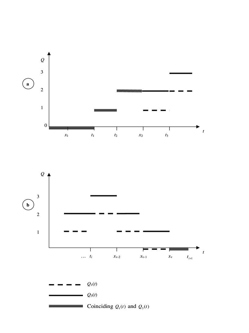
Figure 1. Typical sample paths of the queue-length processes $Q_{1}(t)$ and $Q_{3}(t)$:
(a) Sample paths of the queue-length processes after the origin;
(b) Sample paths of the queue-length processes before approaching zero at point $x_{v}$.

Let $v$ be a new number greater than $l$ satisfying the property

$$v=\inf\left\{k>l:Q_{1}(x_{k}-)=0\right\}.$$

(If such a number does not exist, then $v$ equates to infinity. In this case, obviously, $Q_{3}(t,\omega)-Q_{1}(t,\omega)=1$, $t\geq x_{l}$.) Then for all $t$ of the interval $[x_{l},x_{v})$ we have $Q_{3}(t,\omega)-Q_{1}(t,\omega)=1$, while in the point $x_{v}$ itself we arrive at $Q_{1}(x_{v},\omega)=Q_{3}(x_{v},\omega)=0$, see Figure 1 (b).

Thus, we arrived at zeroth queue-lengths again. The further paths of the both processes after point $t=x_{v}$ behave similarly to those after the point $t=0$, i.e. the difference $Q_{3}(t,\omega)-Q_{1}(t,\omega)$ can take only one of the two values 0 or 1. ∎

From Propositions 3.1 and 3.2 we arrive at the following conclusion: if the queueing system $\mathscr{Q}_{1}$ is stable, then the both queueing systems $\mathscr{Q}_{2}$ and $\mathscr{Q}_{3}$ are stable as well. Following Proposition 3.1 this statement of stability can be extended for more complicated constructions including two, three and more different arrival processes and can be then applied to queueing networks.

4. Stability of JS-queues

In this section we study stability of JS-queues. We start from the simplest case of symmetric $\Sigma_{m}$ queues. Denote $D_{a}(t)=\sum_{j=1}^{m}D_{a}^{(j)}(t)$. In Theorem 4.1 below, the assumption that the processes $A(t)$, $A^{\prime}(t)$ and $D^{(j)}(t)$, $j=1,2,\ldots,m$, all are mutually independent point processes is relaxed. For $\Sigma_{m}$ queues where $p_{j}=\frac{1}{m}$, $j=1,2,\ldots,m$, instead of (2.1), (2.2) and (2.3) we assume

$$\mathbf{P}\left\{\lim_{a\to~{}-\infty}\frac{A_{a}(t)+A_{a}^{\prime}(t)-D_{a}(t)}{t-a}={\lambda+\lambda^{\prime}-\mu m}\right\}=1.$$ (4.1)

Theorem 4.1.

In addition to (4.1) assume that

$$\lim_{a\to~{}-\infty}\mathbf{P}\{A_{a}(t)+A_{a}^{\prime}(t)-D_{a}(t)\in\mathscr{S}\}=0$$ (4.2)

for any bounded set $\mathscr{S}$. Then, the system $\Sigma_{m}$ is stable if and only if the condition $\frac{\lambda}{m}+\frac{\lambda^{\prime}}{m}<\mu$ is fulfilled.

Proof.

Since the families $\{A_{a}^{(j)}(t)\}_{j\leq m}$ and $\{D_{a}^{(j)}(t)\}_{j\leq m}$ consist of identically distributed processes, then the family $\{A_{a}^{\prime(j)}(t)\}_{j\leq m}$ also consists of identically distributed processes, and according to (2.4) the family of the processes $\{Q_{a}^{(j)}(t)\}_{j\leq m}$ consists of identically distributed processes too. Observe that from (4.2), because the system $\Sigma_{m}$ is symmetric, we also have

$$\lim_{a\to~{}-\infty}\mathbf{P}\{A_{a}^{(j)}(t)+A_{a}^{\prime(j)}(t)-D_{a}^{(j)}(t)\in\mathscr{S}\}=0$$ (4.3)

for all $j=1,2,\ldots,m$.

Notice, that if $\frac{\lambda}{m}+\frac{\lambda^{\prime}}{m}<\mu$, then

$$\mathbf{P}\Big{\{}\sup_{a\leq t<\infty}\big{[}A_{a}^{(j)}(t)+A_{a}^{\prime(j)}(t)-D_{a}^{(j)}(t)]<\infty\Big{\}}=1.$$ (4.4)

Indeed, according to (4.1), $\mathbf{P}$-a.s.

$$\lim_{a\to~{}-\infty}\frac{A_{a}^{(j)}(t)+A_{a}^{\prime(j)}(t)-D_{a}^{(j)}(t)}{t-a}=\frac{\lambda}{m}+\frac{\lambda^{\prime}}{m}-\mu<0.$$ (4.5)

Hence, $\mathbf{P}$-a.s.

$$\lim_{a\to~{}-\infty}[A_{a}^{(j)}(t)+A_{a}^{\prime(j)}(t)-D_{a}^{(j)}(t)]=-\infty,$$

and (4.4) follows from the fact that $A_{a}^{(j)}(t)$, $A_{a}^{\prime(j)}(t)$ and $D_{a}^{(j)}(t)$ all are cádlág processes.

Next, taking into account (4.5) and $A_{a}^{(j)}(a)=A_{a}^{\prime(j)}(a)=D_{a}^{(j)}(a)=0$, for the queue-length process $Q^{(j)}(t)$ one can write the following representation:

$$Q_{a}^{(j)}(t)=\big{[}A_{a}^{(j)}(t)+A_{a}^{\prime(j)}(t)-D_{a}^{(j)}(t)\big{]}-\inf_{a\leq s\leq t}\big{[}A_{a}^{(j)}(t)+A_{a}^{\prime(j)}(t)-D_{a}^{(j)}(t)\big{]}.$$ (4.6)

Representation (4.6) is well-known (e.g. Borovkov [10]) and is a consequence from the Skorokhod reflection principle (e.g. Kogan and Liptser [32] for typical application to queue-length processes).

Next, from (4.6) we have:

$$Q_{a}^{(j)}(t) {\buildrel d\over{=}} \sup_{a\leq s\leq t}\big{\{}\big{[}A_{a}^{(j)}(t)+A_{a}^{\prime(j)}(t)-D_{a}^{(j)}(t)\big{]}$$ (4.7)

$$-\big{[}A_{a}^{(j)}(s)+A_{a}^{\prime(j)}(s)-D_{a}^{(j)}(s)\big{]}\}.$$

From representation (4.7), relation (4.4) and the fact that all of the processes $A_{a}^{(j)}(t)$, $A_{a}^{\prime(j)}(t)$ and $D_{a}^{(j)}(t)$ are cádlág processes, it follows that there exists a bounded set $\mathscr{S}_{0}$ such that

$$\limsup_{a\to~{}-\infty}\mathbf{P}\{Q^{(j)}(t)\in\mathscr{S}_{0}\}>0,$$

and the sufficient condition is therefore proved. The necessary condition follows from the fact that (4.3) together with (4.4) imply the condition $\frac{\lambda}{m}+\frac{\lambda^{\prime}}{m}<\mu$. ∎

Remark 4.2.

If $\frac{\lambda}{m}+\frac{\lambda^{\prime}}{m}=\mu$, and the processes $A(t)$, $A^{\prime}(t)$ and $D(t)$ all are non-trivial renewal processes, then we easily arrive at condition (4.2). However, there are examples where $\frac{\lambda}{m}+\frac{\lambda^{\prime}}{m}=\mu$, but condition (4.2) is not fulfilled. Indeed, let $\tau_{1}+\tau_{1}^{\prime}-\chi_{1}$ be a uniformly distributed random variable in $[-b,b]$, ($b>0$), and let $\tau_{i+1}+\tau_{i+1}^{\prime}-\chi_{i+1}=-(\tau_{i}+\tau_{i}^{\prime}-\chi_{i})$, $i\geq 1$. In this case (4.2) is not valid. Therefore condition (4.2) is meaningful.

Remark 4.3.

The conditions of Theorem 4.1 are weaker than conditions of other known stability theorems (e.g. Borovkov [10]) requiring the strict stationarity and ergodicity of appropriate sequence of random variables. For example, assume that the sequence $\{\tau_{n}+\tau_{n}^{\prime}-\chi_{n}\}_{n\geq 1}$ consists of identically distributed random variables, $\tau_{1}+\tau_{1}^{\prime}-\chi_{1}$ is a uniformly distributed random variable in $[-b,b]$, ($b>0$), and $\tau_{2}+\tau_{2}^{\prime}-\chi_{2}=\tau_{1}+\tau_{1}^{\prime}-\chi_{1}$, and $\tau_{i+1}+\tau_{i+1}^{\prime}-\chi_{i+1}=-(\tau_{i}+\tau_{i}^{\prime}-\chi_{i})$, $i\geq 2$. Then the above sequence $\{\tau_{n}+\tau_{n}^{\prime}-\chi_{n}\}_{n\geq 1}$ is not strictly stationary. However, the queueing system associated with this sequence is stable.

For following Theorem 4.4, our assumptions regarding the point processes $A_{a}(t)$, $D_{a}^{(j)}(t)$ is as follows. For dependent processes $A_{a}(t)$, $D_{a}^{(j)}(t)$ we suppose that the normalized processes $\frac{A_{a}(t)}{t-a}$ and $\frac{D_{a}^{(j)}(t)}{t-a}$ converge, as $a\to~{}-\infty$, to the corresponding limits $\lambda$ and $\mu$ only in distribution, while

$$\mathbf{P}\left\{\lim_{a\to~{}-\infty}\frac{A_{a}(t)-D_{a}^{(j)}(t)}{t-a}=\lambda-\mu\right\}=1.$$ (4.8)

Then, the process $A_{a}^{\prime}(t)$ is assumed to satisfy the condition

$$\mathbf{P}\left\{\lim_{a\to~{}-\infty}\frac{A_{a}^{\prime}(t)}{t-a}=\lambda^{\prime}\right\}=1.$$ (4.9)

Next Theorem 4.4 is related to stability of $\wp_{m}$ queues. Denote $\lambda_{j}=\lambda p_{j}$, $j^{*}=\arg\max_{1\leq j\leq m}\lambda_{j}$ and $\Delta=\sum_{j=1}^{m}(\lambda_{j^{*}}-\lambda_{j})$.

Theorem 4.4.

In addition to (4.8) and (4.9) assume that both

$$\lim_{a\to~{}-\infty}\mathbf{P}\{A_{a}(t)+A_{a}^{\prime}(t)-D_{a}(t)\in\mathscr{S}\}=0,$$ (4.10)

and

$$\lim_{a\to~{}-\infty}\mathbf{P}\{A_{a}^{(j^{*})}(t)-D_{a}^{(j^{*})}(t)\in\mathscr{S}\}=0$$ (4.11)

for any bounded set $\mathscr{S}$. Then the system is stable if and only if one of the following two conditions is fulfilled:

$$\begin{cases}\lambda^{(j^{*})}<\mu,&\mbox{if}\ \Delta\geq\lambda^{\prime},\\ \lambda+\lambda^{\prime}<m\mu,&\mbox{otherwise}.\end{cases}$$

Proof.

The theorem can be proved by a slight modification of the earlier proof.

Suppose first that $\Delta\geq\lambda^{\prime}$, and denote $q_{j}$ the fraction of customer of the opportunistic traffic being assigned to the $j$th queue. From the limiting relations

$$\lim_{a\to~{}-\infty}\frac{A_{a}^{(j)}(t)}{t-a} {\buildrel d\over{=}} \lambda_{j},$$

$$\lim_{a\to~{}-\infty}\frac{A_{a}^{\prime(j)}(t)}{t-a} {\buildrel a.s.\over{=}} \lambda_{j}^{\prime},$$

according to well-known Skorokhod’s theorem [50], p. 281, one can conclude that there exists a probability space $(\Omega,\mathscr{F},\mathbf{P})$, with given there a family of processes $\left\{\frac{A_{a}^{(j)}(t,\omega)+A_{a}^{\prime(j)}(t,\omega)}{t-a},t>a\right\}$ such that for $\mathbf{P}-$ almost all $\omega\in\Omega$,

$$\lim_{a\to~{}-\infty}\frac{A_{a}^{(j)}(t,\omega)+A_{a}^{\prime(j)}(t,\omega)}{t-a} = \lambda_{j}+\lambda_{j}^{\prime}.$$

Therefore, from the balance equations

$$\lambda_{j}+\lambda_{j}^{\prime}=\lambda_{j}+\lambda^{\prime}q_{j}=\varrho,$$

one can conclude that $q_{j^{*}}$ must be equal to 0. Therefore

$$\lambda_{j^{*}}\geq\lambda_{j}+\lambda_{j}^{\prime}$$

for all $j=1,2,\ldots,m$, where $\lambda_{j}^{\prime}=\lambda^{\prime}q_{j}$. Then, in this probability space for $\mathbf{P}-$ almost all $\omega\in\Omega$,

$$\lim_{a\to~{}-\infty}\frac{A_{a}^{(j)}(t,\omega)+A_{a}^{\prime(j)}(t,\omega)}{t-a}\leq\lim_{a\to~{}-\infty}\frac{A_{a}^{(j^{*})}(t,\omega)}{t-a},$$

and, from (2.5) and coupling arguments of sample paths comparison

$$\lim_{a\to~{}-\infty}\frac{Q_{a}^{(j)}(t,\omega)}{t-a}\leq\lim_{a\to~{}-\infty}\frac{Q_{a}^{(j^{*})}(t,\omega)}{t-a}.$$

Therefore, in the original probability space we have

$$\lim_{a\to~{}-\infty}\frac{A_{a}^{(j)}(t)+A_{a}^{\prime(j)}(t)}{t-a}~{}{\buildrel d\over{\leq}}~{}\lim_{a\to~{}-\infty}\frac{A_{a}^{(j^{*})}(t)}{t-a},$$

and consequently,

$$\lim_{a\to~{}-\infty}\frac{Q_{a}^{(j)}(t)}{t-a}~{}{\buildrel d\over{\leq}}~{}\lim_{a\to~{}-\infty}\frac{Q_{a}^{(j^{*})}(t)}{t-a}$$

for all $j=1,2,\ldots,m$. Hence the problem reduces to conditions of stability of a single queueing system with autonomous service mechanism with the given arrival process $A^{(j^{*})}(t)$ and departure process $D^{(j^{*})}(t)$, and under assumptions (4.8) and (4.11) the necessary and sufficient condition of stability is given by $\lambda_{j^{*}}<\mu$.

Let us now consider the opposite case $\Delta<\lambda^{\prime}$ and assumption $\lambda+\lambda^{\prime}<\mu m$. Then, there exist probabilities $q_{j}$, $j=1,2,\ldots,m$, all strictly positive, and $\sum_{j=1}^{m}q_{j}=1$. Under these probabilities, the opportunistic traffic is thinned into $m$ processes such that almost surely

$$\lim_{a\to~{}-\infty}\frac{A_{a}^{\prime(j)}(t)}{t-a}=\lambda^{\prime}q_{j}=\lambda_{j}^{\prime}.$$

Indeed, since $\lambda+\lambda^{\prime}<\mu m$, then there exists the value $\varrho=\frac{\lambda+\lambda^{\prime}}{m}<\mu$ such that for all $j$

$$\varrho>\lambda_{j},$$

and therefore,

$$q_{j}=\frac{\varrho-\lambda_{j}}{\lambda^{\prime}}>0.$$ (4.12)

Since $\lambda_{j}+q_{j}\lambda^{\prime}=\varrho$, the family $\left\{A_{a}^{(j)}(t)+A_{a}^{\prime(j)}(t)\right\}_{j\leq m}$ consists of processes having the same rate, i.e.

$$\lim_{a\to~{}-\infty}\frac{A_{a}^{(j)}(t)+A_{a}^{\prime(j)}(t)}{t-a}~{}{\buildrel d\over{=}}~{}\varrho.$$ (4.13)

The possible values $\{q_{j}\}_{j\leq m}$ are unique, since otherwise, if there are different arrival rates $\lambda_{j}+\lambda^{\prime}q_{j}^{\prime}$, then one of queues must be stochastically longer than other. Let $j^{*}$ be the order number of the longer queue. Then $q_{j^{*}}$ should be equal to 0, and we have the contradiction with (4.12).

According to (4.13) for each of $m$ queue-length processes the arrival rate is the same. With the same arrival and departure intensities one can repeat the proof of Theorem 4.1 for each queue-length process. Therefore, $\varrho<\mu$ is the condition for stability, and under condition (4.10) the system is stable if and only if $\varrho<\mu$. The theorem is proved. ∎

Remark 4.5.

In the case of the model $\Gamma_{m}$ the following additional comments are necessary. If the value $j^{*}$ is not unique, then condition (4.11) should be assumed for all $j^{*}$. In addition, instead of condition (4.8) we should require

$$\mathbf{P}\left\{\lim_{a\to~{}-\infty}\frac{A_{a}^{(j)}(t)-D_{a}^{(j)}(t)}{t-a}=\lambda_{j}-\mu\right\}=1$$

for all $j=1,2,\ldots,m$, and in addition we should require the convergence of the normalized processes $\frac{A_{a}^{(j)}(t)}{t-a}$ and $\frac{D_{a}^{(j)}(t)}{t-a}$, as $a\to~{}-\infty$, to the corresponding numbers $\lambda_{j}$ and $\mu$ in distribution.

5. Load-balanced networks and their stability

In the previous section, the necessary and sufficient conditions for stability of systems $\wp_{m}$ have been established. In this section we extend above Theorem 4.4 for load-balanced networks associated with $\wp_{m}$ queueing systems. The main result of this section is Theorem 5.3 establishing the necessary and sufficient condition for the stability of load-balanced networks. Theorems 5.1 and 5.2 are the preliminary results establishing only sufficient conditions for the stability.

The load-balanced network considered below is the following extension of the $\wp_{m}$ queueing system.

Assume that an arriving customer of the dedicated traffic occupies the server $j$ with probability $p_{j}$  ($j=1,2,\ldots,m$), and $\sum_{j=1}^{m}p_{j}=1$. After his service completion in the $j$th queue, a customer leaves the system with probability $1-p_{j}^{*}$, remains at the same $j$th queue with probability $p_{j,j}$, goes to the different queue $i\neq j$ with probability $p_{j,i}$, and choose the shortest queue with probability $p_{j,sh}$, breaking ties at random. It is assumed that $p_{j}^{*}<1$ at least for one of the indexes $j$. This model is called load-balanced network. The stability conditions of the Markovian variant of this network containing two stations only has been established by Kurkova [33].

Some different variants of this network have also been studied in Martin and Suhov [37], Vvedenskaya Dobrushin and Karpelevich [53] and other papers.

Denote $\lambda_{j}=\lambda p_{j}$, $\Lambda_{j}=\lambda_{j}+\mu\sum_{i=1}^{m}p_{i,j}$, $j^{*}=\arg\max_{1\leq j\leq m}\Lambda_{j}$.

For the sake of simplification of the proofs, we follow the assumptions that are described in Section 2, with understanding that they can be relaxed by the way of the previous section. We also assume that the processes all are started at $a$ and use the variants of the assumptions where $a\to~{}-\infty$ rather than $t\to\infty$.

The sufficient condition given in Theorem 5.1 is a straightforward extension of earlier Theorem 4.4 written now in a simpler form.

Theorem 5.1.

Assume that $\lambda_{j^{*}}\geq\Lambda_{j}$ for all $j\neq j^{*}$. Denote

$$\Delta_{1}=\sum_{j=1}^{m}(\Lambda_{j^{*}}-\lambda_{j}),$$

and

$$\Delta_{2}=\sum_{j\neq j^{*}}(\lambda_{j^{*}}-\Lambda_{j}).$$

Then the load-balanced network is stable if one of the following two conditions is fulfilled:

$$\begin{cases}\Lambda_{j^{*}}<\mu,&\mbox{if}\ \Delta_{2}\geq\lambda^{\prime}+\mu\sum_{j=1}^{m}p_{j,sh},\\ \lambda+\lambda^{\prime}+\mu\Big{(}\sum_{i=1}^{m}\sum_{j=1}^{m}p_{i,j}+\sum_{j=1}^{m}p_{j,sh}\Big{)}<m\mu,&\mbox{if}\ \Delta_{1}<\lambda^{\prime}.\end{cases}$$

Proof.

The proof of the theorem starts from the case $p_{j,sh}=0$ for all $j=1,2,\ldots,m$ and then discusses the case $p_{j,sh}\geq 0$ for all $j=1,2,\ldots,m$.

Let us start from the case where $p_{j,sh}=0$ for all $j=1,2,\ldots,m$. Then, the system of equations for the queue-length processes started at $t=a$ can be written

$$Q_{a}^{(j)}(t)=A_{a}^{(j)}(t)+A_{a}^{\prime(j)}(t)+E_{a}^{(j)}(t)-\int_{a}^{t}\mathbf{1}_{\{Q_{a}^{(j)}(s-)>0\}}\mbox{d}D_{a}^{(j)}(s),$$ (5.1)

where the new process $E_{a}^{(j)}(t)$ presenting in (5.1) is a process, generated by internal dedicated arrivals to the $j$th queue. By internal dedicated arrivals to the $j$th queue we mean internal arrivals of the customers, who after their service completion in one or other queue are assigned to the $j$th queue. Recall that there is probability $p_{i,j}$ to be assigned from the queue $i$ to the queue $j$. Relationship (5.1) is of the same type as that (2.5), and therefore all of the arguments of the earlier proof of Theorem 4.4 can be repeated. Specifically, in the case $\Delta_{2}\geq\lambda^{\prime}$ the system is stable if $\Lambda_{j^{*}}<\mu$.

In turn, the process $E_{a}^{(j)}(t)$ can be represented as $\sum_{i=1}^{m}E_{a}^{(i,j)}(t)$, where the point process $E_{a}^{(i,j)}(t)$ is generated by the customers who are assigned to the $j$th queue after their service completion in the $i$th queue (in the case $i=j$ it is assumed that the customers decide to stay at the same queue). Notice, that

$$\lim_{a\to~{}-\infty}\frac{E_{a}^{(i,j)}(t)}{t-a}$$

does exist with probability 1 (because the process $E_{a}^{(i,j)}(t)$ is generated by the procedure of thinning of the departure process $D_{a}^{(i)}(t)$), and

$$\mathbf{P}\Big{\{}\lim_{a\to~{}-\infty}\frac{E_{a}^{(i,j)}(t)}{t-a}\leq\mu p_{i,j}\Big{\}}=1,$$ (5.2)

where the equality holds only in the case where the fraction of the $i$th queue idle period vanishes as $a\to~{}-\infty$. Therefore under the condition $\Delta_{1}<\lambda^{\prime}$ the system is stable if $\lambda+\lambda^{\prime}+\mu\sum_{i=1}^{m}\sum_{j=1}^{m}p_{i,j}<m\mu$.

Assume now that $p_{j,sh}\geq 0$ for all $j=1,2,\ldots,m$. Then instead of (5.1) we have the equation

$$Q_{a}^{(j)}(t) =A_{a}^{(j)}(t)+A_{a}^{\prime(j)}(t)+E_{a}^{(j)}(t)+E_{a}^{\prime(j)}(t)$$ (5.3)

$$\ \ \ -\int_{a}^{t}\mathbf{1}_{\{Q_{a}^{(j)}(s-)>0\}}\mbox{d}D_{a}^{(j)}(s),$$

where $E^{\prime(j)}(t)$ are the point processes associated with internal opportunistic traffic to the $j$th queue. By internal opportunistic traffic we mean the internal traffic of customers presenting in the queue, who after their service completion decide to join the shortest queue. In the case where the shortest queue is the $j$th queue, we say about opportunistic traffic to the $j$th queue. Again,

$$\lim_{a\to~{}-\infty}\frac{E_{a}^{\prime(j)}(t)}{t-a}$$

does exist with probability 1 (because the process $E_{a}^{\prime(j)}(t)$ is generated by the procedure of thinning of the departure process $D_{a}^{(j)}(t)$), and similarly to (5.2) we have:

$$\mathbf{P}\left\{\lim_{a\to~{}-\infty}\frac{\sum_{j=1}^{m}E_{a}^{\prime(j)}(t)}{t-a}\leq\mu\sum_{j=1}^{m}p_{j,sh}\right\}=1.$$ (5.4)

Therefore, the entire opportunistic traffic to the $j$th queue, being a sum of the processes $A_{a}^{\prime(j)}(t)$ and $E_{a}^{\prime(j)}(t)$, satisfies

$$\mathbf{P}\left\{\lim_{a\to~{}-\infty}\frac{\sum_{j=1}^{m}[A_{a}^{\prime(j)}(t)+E_{a}^{\prime(j)}(t)]}{t-a}\leq\lambda^{\prime}+\mu\sum_{j=1}^{m}p_{j,sh}\right\}=1.$$ (5.5)

Hence the proof of this theorem remains similar to the proof of Theorem 4.4. In the case $\Delta_{2}\geq\lambda^{\prime}+\mu\sum_{j=1}^{m}p_{j,sh}$ the system is stable if $\Lambda_{j^{*}}<\mu$. In the other case $\Delta_{1}<\lambda^{\prime}$ the system is stable if $\lambda+\lambda^{\prime}+\mu\Big{(}\sum_{i=1}^{m}\sum_{j=1}^{m}p_{i,j}+\sum_{j=1}^{m}p_{j,sh}\Big{)}<m\mu$. The conditions of the theorem are sufficient and not necessary, because the left-hand sides of (5.2), (5.4) and (5.5) contain the probability of inequalities, and the exact parameters of internal dedicated traffic as well as internal opportunistic traffic are unknown. ∎

In order to formulate and prove a necessary and sufficient condition of stability for the above load-balanced network, we first need to improve the sufficient condition given by Theorem 5.1. For this purpose, rewrite (5.2) as

$$\mathbf{P}\Big{\{}\lim_{a\to~{}-\infty}\frac{E_{a}^{(i,j)}(t)}{t-a}=\varrho_{i}\mu p_{i,j}\Big{\}}=1,$$

where the value $\varrho_{i}$ satisfies the inequality $0<\varrho_{i}\leq 1$. The value $\varrho_{i}$ is the fraction of time when the server of the $i$th queue is busy. Then the case of $\varrho_{i}=1$ means that the server of the $i$th queue is busy almost always.

Let us consider the system of inequalities

$$\frac{\lambda_{j}+\mu\sum_{i=1}^{m}\varrho_{i}p_{i,j}}{\varrho_{j}^{*}}\leq\mu,\ j=1,2,\ldots,m.$$ (5.6)

The meaning of inequality (5.6) is the following. The left-hand side contains the total sum of rates of dedicated traffic to the $j$th queue divided to the traffic parameter $\varrho_{j}^{*}$ of the $j$th queue. The total sum of rates of dedicated traffic of the $j$th queue consists of exogenous and internal arrivals to that $j$th queue, excluding the rates for joining the shortest queue customers. Since the rates associated with opportunistic traffic are excluded, there is the inequality ’$\leq$’ between the left and right sides. Thus, if the $j$th queue is never shortest, then the sum of the rates of the left-hand side divided to $\varrho_{j}^{*}$ becomes equal to $\mu$ of the right-hand side. When the traffic parameter $\varrho_{j}^{*}$ is greater than 1, the $j$th queue increases to infinity with probability 1. Therefore, in the sequel we only consider the case when $\varrho_{j}^{*}\leq 1$ for all $j=1,2,\ldots,m$. In this case $\varrho_{j}^{*}=\varrho_{j}$, and we therefore have

$$\lambda_{j}+\mu\sum_{i=1}^{m}\varrho_{i}p_{i,j}\leq\varrho_{j}\mu,\ j=1,2,\ldots,m.$$ (5.7)

Let us now write a so-called balance equation, taking into account also joining the shortest queue customers. We have

$$\lambda+\lambda^{\prime}+\mu\sum_{j=1}^{m}\sum_{i=1}^{m}\varrho_{i}p_{i,j}=\mu\sum_{j=1}^{m}\varrho_{j}(1-p_{j,sh}).$$ (5.8)

Now, we are ready to prove the improved sufficient condition for the stability. This version is also based on a straightforward extension of Theorem 4.4.

Theorem 5.2.

The load-balanced network is stable if there exists

$$\varrho^{*}=\max_{1\leq j\leq m}\varrho_{j},$$

satisfying the condition $\varrho^{*}<1$, where the values $\varrho_{j}$, $j=1,2,\ldots,m$, are defined by (5.7) and (5.8).

Proof.

Let $\Lambda_{j}=\lambda_{j}+\mu\sum_{i=1}^{m}\varrho_{i}p_{i,j}$, let $j^{*}=\arg\max_{1\leq j\leq m}\Lambda_{j}$, and let $\Delta=\sum_{j=1}^{m}(\Lambda_{j^{*}}-\Lambda_{j})$. In the case $\Delta>\lambda^{\prime}+\mu\sum_{j=1}^{m}\varrho_{j}p_{j,sh}$ the $j^{*}$-th queue is never shortest, and therefore, following the proof of Theorem 4.4, the system is stable if $\Lambda_{j^{*}}<\mu$. Therefore from (5.6) we have $\varrho_{j^{*}}<1$, and because the $j^{*}$-th queue is the longest queue, we have $\varrho^{*}=\varrho_{j^{*}}\geq\varrho_{j}$, $j=1,2,\ldots,m$. Therefore $\varrho_{j}<1$ for all $j=1,2,\ldots,m$ is a sufficient condition of stability for this case.

Let us now consider the opposite case, where $\Delta\leq\lambda^{\prime}+\mu\sum_{j=1}^{m}\varrho_{j}p_{j,sh}$. As in the proof of Theorem 4.4, in this case the arrival rate to all $m$ queues is the same, and therefore $\varrho_{1}=\varrho_{2}=\ldots=\varrho_{m}$. Thus, the only two cases are there as $\varrho_{j}<1$ or $\varrho_{j}=1$ for all $j=1,2,\ldots,m$. In the case $\varrho_{j}<1$, the stability result is analogous to that of Theorem 4.4, since in this case from (5.8) we obtain

$$\lambda+\lambda^{\prime}+\mu\sum_{j=1}^{m}\sum_{i=1}^{m}p_{i,j}+\mu\sum_{j=1}^{m}p_{j,sh}<m\mu.$$

The theorem is proved. ∎

Now in order to formulate and prove a necessary and sufficient condition for stability, let us consider the following linear programming problem in $\mathbb{R}^{m+1}$:

$$\mbox{Minimize}\ x_{m+1}$$ (5.9)

subject to the restrictions:

$$\lambda_{j}+\mu\sum_{i=1}^{m}x_{i}p_{i,j}\leq x_{j}\mu,\ j=1,2,\ldots,m,$$ (5.10)

$$\lambda+\lambda^{\prime}+\mu\sum_{j=1}^{m}\sum_{i=1}^{m}x_{i}p_{i,j}=\mu\sum_{j=1}^{m}x_{j}(1-p_{j,sh}),$$ (5.11)

$$x_{j}\leq x_{m+1},\ j=1,2,\ldots,m.$$ (5.12)

Observe, that the restrictions (5.10) and (5.11) correspond to (5.7) and (5.8), where the values $\varrho_{j}$ are replaced with unknown $x_{j}$. The functional of (5.9) and inequalities (5.12) are associated with the condition of Theorem 5.2: $\max_{1\leq j\leq m}\varrho_{j}<1$. $x_{m+1}$ is an additional variable; thus the linear programming (5.9)-(5.12) is a mini-max problem. That is, if the minimum of $x_{m+1}$ is achieved in some point $x_{m+1}^{*}<1$, then all components of the vector ($x_{1}^{*},x_{2}^{*},\ldots,x_{m+1}^{*}$) associated with this solution are less than 1, and there exists a solution of system (5.7) and (5.8) with $\varrho_{j}<1$ for all $j=1,2,\ldots,m$. Therefore in the following the vector associated with solution of the problem (5.9)-(5.12) is denoted ($\varrho_{1},\varrho_{2},\ldots,\varrho_{m}$). Otherwise if $x_{m+1}^{*}\geq 1$, then we set $\varrho_{j}=1$, $j=1,2,\ldots,m$.

Next, denote $A_{a}^{(j)}(t)+E_{a}^{(j)}(t)$ the dedicated arrival process. Its relation to the initial processes $A_{a}(t)$ and $D_{a}^{(j)}(t)$ is the following. Each arrival of the initial process $A_{a}(t)$ is forwarded to the queue $j$ with probability $p_{j}$, and each customer served in the queue $i$ returns to the $j$th queue with probability $p_{i,j}$. Then, the process $A_{a}^{(j)}(t)+E_{a}^{(j)}(t)$ is a sum of all arrivals of external and internal dedicated traffic, and

$$\mathbf{P}\Big{\{}\lim_{a\to~{}-\infty}\frac{A_{a}^{(j)}(t)+E_{a}^{(j)}(t)}{t-a}=\Lambda_{i}=\lambda_{j}+\mu\sum_{i=1}^{m}\varrho_{i}p_{i,j}\Big{\}}=1,$$

where $\varrho_{j}$, $j=1,2,\ldots,m$, are a solution of the linear programming given by (5.9)-(5.12). Now let $j^{*}=\arg\max_{1\leq j\leq m}\Lambda_{j}$. We have the following theorem.

Theorem 5.3.

Assume that the both

$$\lim_{a\to~{}-\infty}\mathbf{P}\{A_{a}^{(j^{*})}(t)+E_{a}^{(j^{*})}(t)-D_{a}^{(j^{*})}(t)\in\mathscr{S}\}=0,$$ (5.13)

and

$$\lim_{a\to~{}-\infty}\mathbf{P}\{A_{a}(t)+A_{a}^{\prime}(t)+E_{a}(t)+E_{a}^{\prime}(t)-D_{a}(t)\in\mathscr{S}\}=0,$$ (5.14)

for any bounded set $\mathscr{S}$, where $E_{a}(t)=\sum_{j=1}^{m}E_{a}^{(j)}(t)$ is the point process associated with all internal arrivals of dedicated traffic, $E_{a}^{\prime}(t)$ is the point process associated with all internal arrivals of opportunistic traffic, $D_{a}(t)=\sum_{j=1}^{m}D^{(j)}(t)$. Then the load-balanced network is stable if and only if $\max_{1\leq j\leq m}\varrho_{j}<1$.

Remark 5.4.

Conditions (5.13) and (5.14) are verifiable conditions. As soon as the linear programming problem is solved and we know the vector of solution $(\varrho_{1},\varrho_{2},\ldots,\varrho_{m})$, the unknown processes $E_{a}(t)$ and $E_{a}^{\prime}(t)$ as well as $E_{a}^{(j)}(t)$ and $E_{a}^{\prime}{}^{(j)}(t)$ can be easily modelled via derivative processes $D_{a}^{(j)}(t)$ ($j=1,2,\ldots,m$). Note also, that above conditions (5.13) and (5.14) are automatically fulfilled if $\max_{1\leq j\leq n}\varrho_{j}<1$.

Remark 5.5.

In the case of the network associated with the model $\Gamma_{m}$ the following additional comment is necessary. If the value $j^{*}$ is not unique, then condition (5.13) should be assumed for all of these values $j^{*}$.

6. Concluding remarks

In this paper we established stability of different type joint-the-shortest-queue models including load-balanced networks. The statements of stability are established under quite general assumptions on arrival and departure processes by reduction to the corresponding models with autonomous service mechanism.

Now we discuss how these results can be extended to the models of queues and networks allowing batch arrivals and batch departures. For this purpose, consider the queueing system with batch arrivals and departures and autonomous service. For this queueing system let $\mathscr{A}(t)$ denote arrival process and let $\mathscr{D}(t)$ departure process, both marked point processes. (All of the processes considered in this section are assumed to start at zero.) For the sake of simplicity suppose that the marks of the point process $\mathscr{D}(t)$ all are of the constant size $c$ ($c$ is a positive integer number), and therefore $\mathscr{D}(t)=cD(t)$. Then, the queue-length process $Q(t)$ has the following representation (see [4]):

$$Q(t)~{}=~{}\mathscr{A}(t)-\sum_{i=1}^{c}\int_{0}^{t}\mathbf{1}_{\{Q(s-)\geq i\}}\mbox{d}D(s).$$

It was shown in [4] that by using Skorokhod’s reflection principle we arrive at equation

$$Q(t){\buildrel d\over{=}}[\mathscr{A}(t)-\mathscr{D}(t)]-\inf_{s\leq t}[\mathscr{A}(s)-\mathscr{D}(s)],$$ (6.1)

which is similar to that of the process with ordinary departures. The assumption, that the marks of departure process are a constant $c$, is specific and associated with concrete models considered in [4]. Representation (6.1) remains in force in general, when a departure process is an arbitrary marked point process with mutually independent identically distributed marks. Representation (6.1) is easily generalized to the case of JS-queue models. Specifically, for the queue-length process in the $j$th server of the model $\wp_{m}$ we have the similar equation

$$Q^{(j)}(t) {\buildrel d\over{=}}[\mathscr{A}^{(j)}(t)+\mathscr{A}^{\prime(j)}(t)-\mathscr{D}^{(j)}(t)]$$ (6.2)

$$\ \ \ -\inf_{s\leq t}[\mathscr{A}^{(j)}(s)+\mathscr{A}^{\prime(j)}(t)-\mathscr{D}^{(j)}(s)],$$

where $\mathscr{A}^{\prime(j)}(t)$ is the corresponding notation for an opportunistic traffic to the $j$th server of the JS-queue model (see ref. (4.6) for comparison). Thus, the case of batch arrivals and departures is a direct extension of the case of ordinary arrivals and departures, and the conditions for stability are similar.

References

- [1] Abramov, V.M. (2000). A large closed queueing network with autonomous service and bottleneck. Queueing Systems, 35, 23-54.
- [2] Abramov, V.M. (2004). A large closed queueing network containing two types of node and multiple customers classes: One bottleneck station. Queueing Systems, 48, 45-73.
- [3] Abramov, V.M. (2006). Analysis of multiserver retrial queueing systems: A martingale approach and an algorithm of solution. Ann. Operat. Res., 141, 19-50.
- [4] Abramov, V.M. (2006). The effective bandwidth problem revisited. arXiv: math 0604.182.
- [5] Akhmarov, I. and Leont’eva, N.P. (1976). Conditions for convergence to limit processes and the strong law of large numbers for queueing systems. Theor. Prob. Appl. 21, 545-556.
- [6] Altman, E. and Borovkov, A.A. (1997). On the stability of retrial queues. Queueing Systems, 26, 343-363.
- [7] Altman, E. and Hordijk, A. (1997). Application of Borovkov’s renovation theory to non-stationary stochastic recursive sequences and their control. Adv. Appl. Prob. 29, 388-413.
- [8] Asmussen, S. and Foss, S.G. (1993). Renovation, regeneration and coupling in multiple-server queues in continuous time. In: Frontiers in Pure and Applied Probability (H.Niemi, G.Högnas, A.N.Shiryaev, A.V.Melnikov eds), 1, 1-6.
- [9] Baccelli, F., and Foss, S. (1994). Stability of Jackson-type queueing networks. Queueing Systems, 17, 5-72.
- [10] Borovkov, A.A. (1976). Stochastic Processes in Queueing Theory. Springer-Verlag, Berlin.
- [11] Borovkov, A.A. (1984). Asymptotic Methods in Queueing Theory. John Wiley, New York.
- [12] Borovkov, A.A. (1986). Limit theorems for queueing networks. I. Theor. Prob. Appl. 31, 413-427.
- [13] Borovkov, A.A. (1987). Limit theorems for queueing networks. II. Theor. Prob. Appl. 32, 257-272.
- [14] Borovkov, A.A. (1998). Ergodicity and Stability of Stochastic Processes. John Wiley, New York.
- [15] Brandt, A., Franken, P. and Lizek, B. (1990). Stationary Stochastic Models, Academie-Verlag/Wiley, Berlin/Chichester.
- [16] Dai, J.G. (1995). On positive Harris recurrence of multiclass queueing networks: a unified approach via fluid limit models. Ann. Appl. Prob., 5, 49-77.
- [17] El-Taha, M. and Stidham, S. (1999). Sample-Path Analysis of Queueing Systems, Kluwer, Dordrecht.
- [18] Flatto, L. (1985). Two parallel queues created by arrivals of two demands. II. SIAM J. Appl. Math. 45, 861-878.
- [19] Flatto, L., and Hahn, S. (1984). Two parallel queues created by arrivals of two demands. SIAM J. Appl. Math. 44, 1041-1053.
- [20] Flatto, L., and McKean, H.P. (1977). Two queues in parallel. Comm. Pure Appl. Math. 30, 255-263.
- [21] Foley, R.D. and McDonald, R.D. (2001). Join-the-shortest-queue: Stability and exact asymptotics. Ann. Appl. Probab. 11, 569-607.
- [22] Foss, S., and Chernova, N. (1991). On the ergodicity of multichannel not fully accessible communication systems. Problems of Information Transmission, 27, 94-99.
- [23] Foss, S., and Chernova, N. (1998). On the stability of partially accessible queue with state-dependent routing. Queueing Systems, 29, 55-73.
- [24] Foss, S.G. and Kalashnikov, V.V. (1991). Regeneration and renovation in queues. Queueing Systems, 8, 211-223.
- [25] Fricker, C. (1986). Etude d’une file GI/G/1 á service autonomé (avec vacances du serveur). Adv. Appl. Prob., 18, 283-286.
- [26] Fricker, C. (1987). Note sur un modele de file GI/G/1 á service autonomé (avec vacances du serveur). Adv. Appl. Prob., 19, 289-291.
- [27] Gelenbe, E. and Iasnogorodski, R. (1980). A queue with server of walking type (autonomous service). Ann. Inst. H. Poincare, 16, 63-73.
- [28] Halfin, S. (1985). The shortest queue problem. J. Appl. Probab. 22, 865-878.
- [29] Kaspi, H. and Mandelbaum, A. (1992). Regenerative closed queueing networks. Stoch. Stoch. Rep., 39, 239-258.
- [30] Kaspi, H. and Mandelbaum, A. (1994). On Harris recurrence in continuous time. Math. Operat. Res., 19, 211-222.
- [31] Kiefer, J. and Wolfowitz, J. (1955). On the theory of queues with many servers. Trans. Amer. Math. Soc. 78, 1-18.
- [32] Kogan, Ya., and Liptser, R.Sh. (1993). Limit non-stationary behavior of large closed queueing network with bottlenecks. Queueing Systems, 14, 33-55.
- [33] Kurkova, I.A. (2001). A load-balanced network with two servers. Queueing Systems, 37, 379-389.
- [34] Kurkova, I.A., and Suhov, Yu.M. (2003). Malyshev’s theory and JS-queues. Asymptotics of stationary probabilities. Ann. Appl. Probab. 13, 1313-1354.
- [35] Lindley, D.V. The theory of queues with a single server. Proc. Cambr. Phil. Soc. 48, 277-289.
- [36] Loynes, R. (1962). The stability of queues with non-independent interarrival and service times. Proc. Cambr. Phil. Soc. 58, 497-520.
- [37] Martin, J.B., and Suhov, Yu.M. (1999). Fast Jackson networks. Ann. Appl. Probab. 9, 854-870.
- [38] Meyn, S.P. and Down, D. (1994). Stability of generalized Jackson networks. Ann. Appl. Prob. 4, 124-148.
- [39] Meyn, S.P. and Tweedie, R.L. (1992). Stability of Markov processes. I. Criteria for discrete time chains. Adv. Appl. Prob., 24, 542-574.
- [40] Meyn, S.P. and Tweedie, R.L. (1993). Stability of Markov processes. II. Continuous time processes and sampled paths. Adv. Appl. Prob., 25, 487-517.
- [41] Meyn, S.P. and Tweedie, R.L. (1993). Stability of Markov processes. III. Foster-Lyapunov criteria for continuous-time processes. Adv. Appl. Prob., 25, 518-548.
- [42] Meyn, S.P. and Tweedie, R.L. (1993). Markov Chains and Stochastic Stability. Springer-Verlag, Berlin.
- [43] Mitzenmacher, M.D. (1996). The power of two choices in randomized load balancing. PhD thesis. University of California at Berkeley.
- [44] Orey, S. (1971). Lecture Notes on Limit Theorems for Markov Chains Transition Probabilities. Van Nostrand Reinhold Co., London.
- [45] Richter, J. (1997). Advanced Windows. Microsoft Press, Redmond, Washington DC.
- [46] Revuz, D. (1975). Markov Chains. Horth-Holland Publiching Co., Amsterdam.
- [47] Rybko, A.N. and Stolyar, A.L. (1992). On the ergodicity of random processes that describe the functioning of open queueing networks. Probl. Inform. Transmiss. 28, 199-220.
- [48] Sharifnia, A. (1997). Instability of the join-the-shortest-queue and FCFS policies in queueing systems and their stabilization. Operations Research, 45, 309-314.
- [49] Sigman, K. (1990). The stability of open queueing networks. Stoch. Proces. Appl. 35, 11-25.
- [50] Skorokhod, A.V. (1956). Limit theorems for stochastic processes. Theor. Prob. Appl., 1, 261-290.
- [51] Suhov, Yu.M., and Vvedenskaya, N.D. (2002). Fast Jackson networks with dynamic routing. Probl. Inform. Transmission, 38, 136-159.
- [52] Tandra, R., Hemachandra, N. and Manjunath, D. (2004). Job minimum cost queue for multiclass customers. Stability and Performance bounds. Probability in the Engineering and informational Sciences, 18, 445-472.
- [53] Vvedenskaya, N.D., Dobrushin, R.L., and Karpelevich, F.I. (1996). A queueing system with selection the shortest of two queues: An asymptotic approach. Probl. Inform. Transmission, 32, 15-27.
- [54] Vvedenskaya, N.D. and Suhov, Yu.M. (2004). Functional equations in asymptotic problems of queueing theory. Journal of Mathematical Sciences (N.Y.), 120, 1255-1276.
- [55] Winston, W. (1977). Optimality of the shortest line discipline. J. Appl. Probab. 14, 181-189.