Abstract

In this paper we prove that parabolic Julia sets of rational functions are locally computable in polynomial time.

1 Introduction

In the present paper we consider the complexity of generating precise images of Julia sets with parabolic orbits. It has been independently proved in [Brv04] and [Ret04] that hyperbolic Julia sets can be computed in polynomial time. Neither of the two algorithms can be applied in the parabolic case. In fact, both algorithms often slow down significantly as the underlying polynomial approaches one with a parabolic point. A naïve generalization of these algorithms would yield exponential time algorithms in the parabolic case, which are useless when one is trying to produce meaningful pictures of the Julia set in question.

The same problem has been highlighted in the comments on computer graphics by John Milnor in [Mil00], Appendix H. The example considered there is for the polynomial $p(z)=z+z^{4}$. It has a parabolic fixed point at $z=0$. Consider a point $z=\varepsilon\approx 1/1000$. Suppose we are trying to determine whether $\varepsilon$ is in the Julia set or not by iterating it, and observing whether its orbit escapes to $\infty$, or converges to $0$. In fact, such a $z$ would always escape to $\infty$, but it is not hard to see that this process would take $1/3\varepsilon^{3}\approx 300,000,000$ iterations for $z$ to escape the ball of radius $2$ around $0$. Thus, we would need to follow the orbit for $\approx 300,000,000$ iterations before concluding that it converges to $\infty$. If we zoom-in a little and set $z=\varepsilon\approx 1/100,000$, we would need $\approx 3\cdot 10^{14}$ iterations to trace $z$, which is computationally impractical.

Due to the effect highlighted above, most computer programs plotting Julia sets include all the points that diverge slowly from the parabolic orbit in the Julia set.

The algorithm we present here is not uniform, i.e. it requires a special program for each specific parabolic Julia set. The running time of the algorithm is $C_{r}n^{c}$, where the constant $C_{r}$ depends on the rational function $r$ but not on $n$, and $c$ is some constant. The algorithm can be made uniform in the $r$, provided some basic combinatorial information about the parabolic points. I.e. one algorithm can compute all the parabolic sets, if it is provided with some basic information about the rational function. The constant $C_{r}$ in the running time can still vary strongly for different functions $r$. For example, it is reasonable to expect that $J_{r_{1}}$ for $r_{1}(z)=z+z^{2}$ would take less time to compute than $J_{r_{2}}$ for $r_{2}(z)=e^{2\pi i/17}z+z^{23}$. We prove the following:

Theorem 1

There is an algorithm $A$ that given

• a rational function $r(z)$ such that every critical orbit of $r$ converges either to an attracting or a parabolic orbit; and

• some basic combinatorial information about the parabolic orbits of $r$;

produces an image of the Julia set $J_{r}$. $A$ takes time $C_{r}n^{c}$ to decide one pixel in $J_{r}$ with precision $2^{-n}$. Here $c$ is some small constant and $C_{r}$ depends on $r$ but not on $n$.

After this work was completed, John Milnor has informed us that he has used an algorithm similar to ours to produce pictures of Julia sets with parabolic points. In particular, some of the pictures in [Mil00] were created this way.

The rest of the paper is organized as follows. In section 2 we give the necessary preliminaries on the complexity theory over the reals. In section 3 we outline the general strategy for computing parabolic Julia sets fast. Sections 4, 5 and 6 provide the main tool for the algorithm – computing a “long” iteration near a parabolic point. Finally, in section 7, we present and analyze the algorithm.

Acknowledgment. The author wishes to thank Ilia Binder and Michael Yampolsky for their insights and encouragement during the preparation of this paper.

2 Complexity over $\mathbbm{R}$ – preliminaries

In this section we provide some preliminaries on the notion of complexity for sets and functions over $\mathbbm{R}^{n}$, in particular $\mathbbm{R}^{2}$. More details can be found in [BW99], [Brv05] and [Wei00].

2.1 Complexity of Sets in $\mathbbm{R}^{2}$

Intuitively, we say the computational complexity of a set $S$ is $t(n)$ if it takes time $t(n)$ to decide whether to draw a pixel of size $2^{-n}$ in the picture of $S$. To make this notion precise, we have to decide what are our expectations from a picture of $S$. First of all, we expect a good picture of $S$ to cover the whole set $S$. On the other hand, we expect every point of the picture to be close to some point of $S$, otherwise the picture would have no descriptive power about $S$. Mathematically, we write these requirements as follows:

Definition 2

A set $T$ is said to be a $2^{-n}$-picture of a bounded set $S$ if

(i) $S\subset T$, and (ii) $T\subset B(S,2^{-n})=\{x\in\mathbbm{R}^{2}~{}:~{}|x-s|<2^{-n}~{}\mbox{for some~{}}s\in S\}$.

Definition 2 is also equivalent to approximating $S$ by $T$ in the Hausdorff metric, given by

$$d_{H}(S,T):=\inf\{r:S\subset B(T,r)~{}~{}\mbox{and}~{}~{}T\subset B(S,r)\}.$$

Suppose we are trying to generate a picture of a set $S$ using a union of round pixels of radius $2^{-n}$ with centers at all the points of the form $\left(\frac{i}{2^{n}},\frac{j}{2^{n}}\right)$, with $i$ and $j$ integers. In order to draw the picture, we have to decide for each pair $(i,j)$ whether to draw the pixel centered at $\left(\frac{i}{2^{n}},\frac{j}{2^{n}}\right)$ or not. We want to draw the pixel if it intersects $S$ and to omit it if some neighborhood of the pixel does not intersect $S$. Formally, we want to compute a function

$$f_{S}(n,i/2^{n},j/2^{n})=\left\{\begin{array}[]{ll}1,&B((i/2^{n},j/2^{n}),2^{-n})\cap S\neq\emptyset\\ 0,&B((i/2^{n},j/2^{n}),2\cdot 2^{-n})\cap S=\emptyset\\ 0~{}~{}\mbox{or}~{}~{}1,{}{}&\mbox{in all other cases}\end{array}\right.$$ (1)

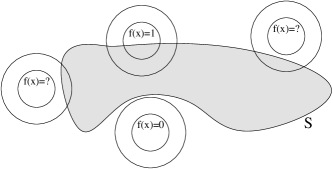
Figure 1: Sample values of $f$. The radius of the inner circle is $2^{-n-2}$.

Lemma 3

The picture drawn according to $f_{S}(n,\bullet)$ is a $2^{-(n-2)}$-picture of $S$.

Here $\bullet$ stands for the different values of the parameters $(i/2^{n},j/2^{n})$. The lemma illustrates the tight connection between the complexity of “drawing” the set $S$ and the complexity of computing $f$. We reflect this connection by defining the time complexity of $S$ as follows.

Definition 4

A bounded set $S$ is said to be computable in time $t(n)$ if there is a function $f(n,\bullet)$ satisfying (1) which runs in time $t(n)$. We say that $S$ is poly-time computable if there is a polynomial $p$, such that $S$ is computable in time $p(n)$.

To see why this is the “right” definition, suppose we are trying to draw a set $S$ on a computer screen which has a $1000\times 1000$ pixel resolution. A $2^{-n}$-zoomed in picture of $S$ has $O(2^{2n})$ pixels of size $2^{-n}$, and thus would take time $O(t(n)\cdot 2^{-2n})$ to compute. This quantity is exponential in $n$, even if $t(n)$ is bounded by a polynomial. But we are drawing $S$ on a finite-resolution display, and we will only need to draw $1000\cdot 1000=10^{6}$ pixels. Hence the running time would be $O(10^{6}\cdot t(n))=O(t(n))$. This running time is polynomial in $n$ if and only if $t(n)$ is polynomial. Hence $t(n)$ reflects the ‘true’ cost of zooming in.

2.2 Computing Julia Sets

There are uncountably many rational functions, but only countably many Turing Machines. Thus, we cannot expect to have a Turing Machine computing the Julia set $J_{r}$ for each rational $r(z)$. Instead, we assume that the coefficients of $r$ are given to the machine, and it is trying to produce a picture of $J_{r}$. The machine can access the coefficients with an arbitrarily high (finite precision). It is charged $m$ time units for querying a coefficient with precision $2^{-m}$. Hence if a machine computes $J_{r}$ with precision $2^{-n}$ in time polynomial $p(n)$, it will query the coefficients with precision at most $2^{-p(n)}$.

Another issue is whether the computation of a machine is uniform or non-uniform. A machine for computing $J_{r}$ is non-uniform, if it is designed specifically for this $r$. A machine is uniform on a set $S$ of rational functions, if it produces $J_{r}$ for all $r\in S$. One can view a non-uniform machine as a uniform machine on the set $S=\{r\}$. One of the properties of the computation model is that if $J_{r}$ is uniformly computable on $S$, then the function $J:r\mapsto J_{r}$ is continuous in the Hausdorff metric. In the case of a non-uniform computation, $S$ is a singleton, and thus we don’t get any information from this statement.

We first give a non-uniform algorithm for computing $J_{r}$. Then in section 7.3 we argue that it can be made uniform for some large classes of parabolic Julia sets. The function $J:r\mapsto J_{r}$ is not continuous over all parabolic sets, and thus it cannot be uniformly computable on all parabolic functions $r$. See section 7.3 for more details.

3 The Strategy

First we recall the strategy in the hyperbolic case, which is much easier to deal with. Suppose that $r$ is a hyperbolic rational function. Let $J_{r}$ denote its Julia set. Then $r$ is strictly expanding by some constant $c>1$ in the hyperbolic metric around $J_{r}$, and thus the escape rate of a point $z\notin J_{r}$ near $J_{r}$ is exponential. In other words, if $d(z,J_{r})>2^{-n}$, then after $O(n)$ steps the orbit of $z$ will be at $\Theta(1)$ distance from $J_{r}$. This gives a natural poly-time algorithm for computing $J_{r}$: iterate $z$ until it is possible to estimate the distance from $r^{k}(z)$ to $J_{r}$ using some coarse initial approximation to $J_{r}$. If such a $k=O(n)$ exists, use $d(r^{k}(z),J_{r})$ and $|(r^{k})^{\prime}(z)|$ to estimate $d(z,J_{r})$. If no such $k$ exists, we can be sure that initially $d(z,J_{r})<2^{-n}$.

We would like to employ a similar strategy here, in the parabolic case. The problem is that even though $r$ is still expanding in the hyperbolic metric near $J_{r}$, the expansion is now extremely slow near the parabolic point. For example, let $r(z)=z^{2}+1/4$, with the parabolic point $p=1/2$. The picture of $J_{r}$ is presented of figure 2. If we set $z=1/2+2^{-n}$, it will take $O(2^{n})$ steps before $z$ escapes the unit disk.

We solve this problem by approximating a “long” iteration of $z$ in the neighborhood of a parabolic point fast. In the previous example “long” would mean $O(2^{n})$.

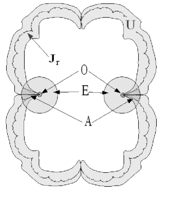
Figure 2: A schematic image of the components in the algorithm.

On figure 2, we present the different regions which will appear in the algorithm. We list them below.

• $J_{r}$ is the Julia set we are trying to compute.

• $U$ is some small fixed region around $J_{r}$. All the points in $U$ are much closer to $J_{r}$ than to the postcritical set. $U$ is bounded away from $J_{r}$, except for a finite number of parabolic and preparabolic touching points. On figure 2 the touching points are $1/2$ (the parabolic point) and $-1/2$ (first-order preparabolic).

• $E$ is the region around the parabolic points in which the “long” iteration is applicable. We also include in $E$ preimages of this neighborhood around the preparabolic touching points of $U$ and $J_{r}$.

• $A\subset U\cup E$ is a collection of small wedges around the repelling directions. These wedges contain the portions of $J_{r}$ in the neighborhood of the corresponding parabolic/preparabolic points.

• $O$ is a tiny neighborhood around the touching points of $U$ and $J_{r}$. If the orbit of $z$ falls into $O$ we can be sure that $z$ is close to $J_{r}$ because all of $O$ is so close to $J_{r}$.

Now the algorithm works exactly as the one in the hyperbolic case:

1. Iterate the orbit of $z$;

2. let $w=r^{k}(z)$ be the current iterate;

3. if $w\notin U\cup E$, we can estimate its distance from $J_{r}$ in $O(1)$ time;

4. if $w\in U-E$, just make one step $w\leftarrow r(w)$;

5. if $w\in O$, output “$w$ close to $J_{r}$”;

6. if $w\in E\cap A$ in the neighborhood of a preparabolic point, just make one step $w\leftarrow r(w)$;

7. if $w\in E-A$, we can estimate its distance from $J_{r}$ in $O(1)$ time;

8. if $w\in E\cap A$ near some parabolic point, apply linearly many “long” iterations to escape this region and get to step 4;

Step 4 can only be executed linearly many times, since $\partial U$ is bounded away from $J_{r}$ outside of $E$ and the expansion in the hyperbolic metric is bounded from below by some $c>1$ on $U-E$. Thus the entire computation takes at most a quadratic number of steps to complete (at most linearly many executions of step 8 between two executions of step 4).

Of course, this is only a sketch, and we need more precise procedures taking into account the finite precision of the computation etc. (e.g. we cannot just check whether $w$ is in $A$ or not.) In the next sections we will develop the tools for performing the “long” iteration near the parabolic points, before formally presenting the algorithm.

4 Controlling coefficient growth

The primary goal of this section is to prove the following lemma.

Lemma 5

Let $r\geq 1$ be some integer. Set $f(z)=z+z^{r+1}+z^{r+2}+z^{r+3}+\ldots$. Then there is an explicit $\alpha$ such that the coefficients of the $n$-th iteration $f^{n}$ of $f$,

$$f^{n}(z)=z+a_{r}z^{r+1}+a_{r+1}z^{r+2}+a_{r+2}z^{r+3}+\ldots,$$

satisfy

$$a_{k}\leq(\alpha n)^{k/r}.$$

One can take $\alpha=2r^{3}$.

We begin with a very simple proof in the case $r=1$. The general case is more involved.

Proof:    (in the case $r=1$.) In this case $f(z)=z+z^{2}+z^{3}+\ldots=\frac{z}{1-z}$ (within the region of convergence). It is easy to verify that

$$f^{n}(z)=\frac{z}{1-nz}.$$

Hence the coefficient of $z^{k+1}$ in $f^{n}$ is $n^{k}$, and lemma 5 holds with $\alpha=1$.  

For the rest of the section we fix some $r\geq 2$, for which we are proving lemma 5. We will prove the lemma by induction on $n$. It is obviously true for $n=1$ with any $\alpha\geq 1$. Denote $\rho=(\alpha n)^{1/r}$. We will find a constant $\alpha$ that works later in the proof, $\alpha$ may depend on $r$ but not on $n$.

If $g(z)$ and $h(z)$ are two power series with positive real coefficients, we say that $g$ is dominated by $h$, and write $g\ll h$ if all the coefficients of $g$ are smaller or equal to the corresponding coefficient of $h$.

We assume by the induction hypothesis that

$$f^{n}(z)\ll z+\rho^{r}z^{r+1}+\rho^{r+1}z^{r+2}+\ldots.$$ (2)

Denote $g(z)=z+rz^{r+1}+rz^{2r+1}+rz^{3r+1}+\ldots$. We claim the following.

Lemma 6

Let $m\geq r$ be a given integer number. Then

$$f(z)^{m}-z^{m}\ll(1+z+z^{2}+\ldots+z^{r-1})\cdot(g(z)^{m}-z^{m}).$$

Proof:    We show that the coefficient of $z^{k}$ on the left hand side is smaller or equal to the coefficient on the right hand side. Note that all the coefficients on the left for $k<m+r$ are $0$, and so we can assume that $k\geq m+r$. Write $k-m=r\cdot l+q$ with $0\leq q<r$, $l\geq 1$. We claim that the coefficient of $z^{k-q}=z^{r\cdot l+m}$ in $g(z)^{m}$ is bigger or equal to the coefficient of $z^{k}$ in $f(z)^{m}$.

To see this we create a one-to-one mapping from all the terms of degree $k$ in the expansion of $f(z)^{m}$ to the corresponding terms of degree $k-q$ in the expansion of $g(z)^{k}$ where we write

$$g(z)=z^{1}_{(0)}+z^{r+1}_{(0)}+z^{r+1}_{(1)}+\ldots+z^{r+1}_{(r-1)}+z^{2r+1}_{(0)}+z^{2r+1}_{(1)}+\ldots+z^{2r+1}_{(r-1)}+\ldots.$$

Here $z_{(0)},\ldots,z_{(r-1)}$ refer to different copies of the same $z$ (we separate the different copies to specify the one-to-one mapping).

Suppose we are given a term $z^{a_{1}}z^{a_{2}}\ldots z^{a_{m}}=z^{k}$ in the expansion of $f(z)^{m}$. We write $a_{i}=1+r\cdot b_{i}+c_{i}$, $0\leq c_{i}<r$. Then we know that either $a_{i}-c_{i}=1$ and $c_{i}=0$, or $a_{i}-c_{i}\geq r+1$. We associate the term

$$z_{(c_{1})}^{a_{1}-c_{1}}z_{(c_{2})}^{a_{2}-c_{2}}\ldots z_{(c_{m-1})}^{a_{m-1}-c_{m-1}}z_{(0)}^{a_{m}+c_{1}+c_{2}+\ldots+c_{k-1}-q}.$$ (3)

By the construction $a_{m}+c_{1}+c_{2}+\ldots+c_{m-1}-q\equiv a_{m}+a_{1}+a_{2}+\ldots+a_{m-1}-(m-1)-q\equiv k-m-q+1\equiv 1~{}(mod~{}r)$. $k\geq m+r$, so we will never need the term $z^{m}$ from $g(z)^{m}$. It is not hard to see that the correspondence is one-to-one, since the information in (3) is sufficient to recover the values of $a_{1},a_{2},\ldots,a_{m}$.

By considering the term $z^{q}\cdot g(z)^{m}$, we complete the proof.  

We are now ready to make the induction step in lemma 5. By the induction hypothesis and lemma 6, we have

$$f^{n+1}(z)\ll f(z)+\rho^{r}z^{r+1}+\rho^{r}(f(z)^{r+1}-z^{r+1})+\rho^{r+1}z^{r+2}+\rho^{r+1}(f(z)^{r+2}-z^{r+2})+\ldots\ll$$

$$f(z)+\rho^{r}z^{r+1}+\rho^{r+1}z^{r+2}+\rho^{r+2}z^{r+3}+\ldots+$$

$$+(1+z+z^{2}+\ldots+z^{r-1})\cdot\left[\rho^{r}(g(z)^{r+1}-z^{r+1})+\rho^{r+1}(g(z)^{r+2}-z^{r+2})+\ldots\right]$$

Our goal is to bound the coefficient of $z^{k}$, $k\geq r+1$, in $f^{n+1}(z)=f^{n}(f(z))$. The contribution from $f(z)$ is always $1$. We consider the contribution from $g(z)^{m}-z^{m}$, $r+1\leq m\leq k$. Write $k=m+r\cdot l+q$, $0\leq q<r$. Then we must have $z^{q}$ in the product, and the coefficient is the coefficient of $z^{m+r\cdot l}$ in $\rho^{m-1}g(z)^{m}$, which is bounded by $\rho^{m-1}{m+l-1\choose l}r^{l}$. The contribution is nonzero only if $l>0$. Thus, the coefficient is bounded by

$$1+\rho^{k-1}+\sum_{q=0}^{r-1}\sum_{l=1}^{\left\lfloor\frac{k-q-r-1}{r}\right\rfloor}\rho^{k-rl-q-1}r^{l}{k-rl-q+l-1\choose l}<$$

$$\rho^{k-1}+r\sum_{l=1}^{\left\lfloor\frac{k-1}{r}\right\rfloor}\rho^{k-rl-1}r^{l}{k-rl+l-1\choose l}<\rho^{k-1}+\sum_{l=1}^{\left\lfloor\frac{k-1}{r}\right\rfloor}\rho^{k-rl-1}r^{l+1}{k-1\choose l}<$$

$$\rho^{k-1}+\rho^{k-1}\sum_{l=1}^{k-1}\rho^{-rl}r^{2l}{k-1\choose l}=\rho^{k-1}\sum_{l=0}^{k-1}\rho^{-rl}r^{2l}{k-1\choose l}=\left(\rho+\frac{r^{2}}{\rho^{r-1}}\right)^{k-1}.$$

To prove the lemma, we need the condition

$$\left(\rho+\frac{r^{2}}{\rho^{r-1}}\right)^{k-1}\leq(\alpha(n+1))^{(k-1)/r}.$$ (4)

Recall that $\rho=(\alpha n)^{1/r}$, hence we can rewrite (4) as

$$\left((\alpha n)^{1/r}+\frac{r^{2}}{(\alpha n)^{(r-1)/r}}\right)^{r}\leq\alpha(n+1).$$

We have

$$\left((\alpha n)^{1/r}+\frac{r^{2}}{(\alpha n)^{(r-1)/r}}\right)^{r}=(\alpha n)\cdot\left(1+\frac{r^{2}}{\alpha n}\right)^{r}<(\alpha n)\cdot e^{\frac{r^{3}}{\alpha n}}<(\alpha n)\cdot\left(1+\frac{2r^{3}}{\alpha n}\right),$$

the last inequality holds whenever $\frac{r^{3}}{\alpha n}<\ln 2$. Finally, if we take $\alpha\geq 2r^{3}$, then

$$(\alpha n)\cdot\left(1+\frac{2r^{3}}{\alpha n}\right)<(\alpha n)\cdot\left(1+\frac{1}{n}\right)=\alpha(n+1),$$

as required.

5 Computing the $n$-th iteration of $f$

Suppose that we are given a function $f$ presented as a power series, finite or infinite, $f(z)=z+a_{2}z^{2}+a_{3}z^{3}+\ldots$, $d\geq 2$. Denote for the $n$-th iteration $f^{n}$ of $f$

$$f^{n}(z)=z+a_{2}^{(n)}z^{2}+a_{3}^{(n)}z^{3}+\ldots$$ (5)

The goal of this section is to show how to compute the values of $a_{k}^{(n)}$ with a given precision $2^{-l}$ fast – in time polynomial in $k$, $l$, and $\log n$. We will need this in order to interpolate “long” iterations of $f$ around the parabolic point ($0$ in this case).

First, we show that if $f$ has a non-negative radius of convergence $R$, then we can assume that $|a_{i}|\leq 1$ for all $i$, with a fairly small overhead. We know that $\sum_{i}a_{i}(R/2)^{i}$ converges. Hence there is a bound $B\geq 1$ such that $a_{i}(R/2)^{i}<B$ for all $i$. In other words, $|a_{i}|<B\cdot(2/R)^{i}\leq(2B/R)^{i}/B$. In case $f$ is a rational function, it is easy to approximate the number $2B/R$, or some power of two $C=2^{c}$, such that $|a_{i}|<C^{i-1}$ for all $i$. Conjugate $f$ by the map $z\mapsto Cz$ to obtain $g(z)=Cf(z/C)$. Then $f(z)=g(Cz)/C$, and $g^{n}(z)=Cf^{n}(z/C)$. The Taylor expansion of $g(z)$ is

$$g(z)=z+\frac{a_{2}}{C}z^{2}+\frac{a_{3}}{C^{2}}z^{3}+\ldots$$

We see that all the coefficients of $g(z)$ do not exceed $1$ in absolute value. The Taylor expansion of the $n$-th iteration of $g$ is

$$g^{n}(z)=z+\frac{a_{2}^{(n)}}{C}z^{2}+\frac{a_{3}^{(n)}}{C^{2}}z^{3}+\ldots$$

Thus, to compute $a_{k}^{(n)}$ with precision $2^{-l}$, we would need to compute the coefficient of $z^{k}$ in $g^{n}$ with precision $2^{-(l+c\cdot k)}$. This is a linear overhead, and if we can compute approximations for $g$ in time $poly(k,l,\log n)$, we will also be able to do it for $f$. From now on, we assume that $|a_{i}|\leq 1$ for all $i$.

We prove the following lemma.

Lemma 7

Suppose $f(z)=z+a_{2}z^{2}+a_{3}z^{3}+\ldots$ is given by its power series. Then the coefficient $a_{k}^{(n)}$ as in (5) can be presented by a polynomial of the form

$$a_{k}^{(n)}=\alpha_{0}^{k}+\alpha_{1}^{k}n+\alpha_{2}^{k}n^{2}+\ldots+\alpha_{k-1}^{k}n^{k-1},$$ (6)

and the values of $\alpha_{i}^{j}$ for $j=2,3,\ldots,k$, $i=0,\ldots,k-1$, can be computed with precision $2^{-s}$ in time polynomial in $k$ and $s$.

Proof:    We prove the lemma by providing an iterative algorithm that computes the values of $\alpha_{i}^{k}$. In the same time we prove that $a_{k}^{(n)}$ is indeed of the form as in equation (6). On the $j$-th iteration we compute the values of $\alpha_{0}^{j}$, $\alpha_{1}^{j}$, …, $\alpha_{j-1}^{j}$.

Here is how to compute the $\alpha_{i}^{j}$ from the $\alpha_{i}^{j-1}$’s. We know that

$$f^{n}(z)=f^{n-1}(f(z))=f(z)+a_{2}^{(n-1)}\cdot f(z)^{2}+a_{3}^{(n-1)}\cdot f(z)^{3}+\ldots$$

In order to compute $a_{j}^{(n)}$ we need to find the coefficient of $z^{j}$ in each of the terms $f(z)$, $f(z)^{2}$, $\ldots$, $f(z)^{j}$ (it is always $0$ in higher terms). All we have to do is to compute all the coefficients of $f(z),f(z)^{2},\ldots,f(z)^{j}$ up to $z^{j}$ with precision $2^{-m}$ in time polynomial in $m$ and $j$.

We assume here that the coefficients $a_{2},a_{3},\ldots,a_{j}$ are given as oracles. In case that $f$ is a rational function

$$f(z)=\frac{z+p(z)\cdot z^{2}}{c-q(z)\cdot z},$$

we know that $c\neq 0$, by the parabolicity of $f$ around $0$, hence

$$f(z)=\frac{1}{c}\cdot\frac{z+p(z)\cdot z^{2}}{1-q(z)\cdot z/c}=\frac{1}{c}\cdot\sum_{k=0}^{\infty}(z+p(z)z^{2})\left(\frac{q(z)\cdot z}{c}\right)^{k}.$$

The first $j$ coefficients of the expansion are now easily computed from this last formula.

The computation is done using a simple “doubling” algorithm: first compute $f(z)^{2}$, $f(z)^{2^{2}}$, $f(z)^{2^{3}}$, $\ldots$, $f(z)^{2^{\left\lfloor\log j\right\rfloor}}$, and then compute the desired power of $f(z)$ as a combination of these. At each multiplication we “chop” all the terms of degree $j+1$ and above, hence the entire computation is polynomial. All the coefficients at all times are bounded by $j^{j}$ in absolute value, hence the error is multiplied by at most $2j^{j}=2^{O(j\log j)}$ at each step, and we will need to do the operations with a precision of $2^{-(m+O(j\log^{2}j))}$ in order for the final coefficients to be with precision $2^{-m}$.

Note that in the case when $f$ is a finite degree polynomial, we can evaluate the coefficients of its powers using the multinomial formula, and with no need for the numerical iterative computation described above.

Once we have the coefficient $c_{j}^{(i)}$ of $z^{j}$ in $f(z)^{i}$, we are able to write

$$a_{j}^{(n)}=a_{j}+a_{2}^{(n-1)}c_{j}^{(2)}+a_{3}^{(n-1)}c_{j}^{(3)}+\ldots+a_{j}^{(n-1)}c_{j}^{(j)}.$$ (7)

We already have all the parameters in (7), as numbers or explicit polynomials in $n$ of degree at most $j-2$, except for $a_{j}^{(n-1)}$. It is easy to see that $c_{j}^{(j)}=1$. Thus, we obtain an explicit recurrence, that connects $a_{j}^{(n)}$ with $a_{j}^{(n-1)}$, and yields

$$a_{j}^{(n)}=a_{j}+\sum_{i=1}^{n-1}\left(a_{j}+a_{2}^{(i)}c_{j}^{(2)}+a_{3}^{(i)}c_{j}^{(3)}+\ldots+a_{j-1}^{(i)}c_{j}^{(j-1)}\right).$$

Thus, $a_{j}^{(n)}$ is given by a polynomial of degree at most $j-1$ in $n$. The coefficients can be computed very efficiently (see [GKP94] for more information on how to compute the sum $\sum_{i=1}^{n}i^{j}$). The precision bit loss in this process is also limited to $O(k\log^{2}k)$ bits. The coefficients of the polynomial $a_{k}^{(n)}$ are precisely the information we are looking for to complete the proof of the lemma.  

6 Computing a “long” iteration

We can now apply the results of sections 4 and 5 to prove the following lemma.

Lemma 8

Suppose $f(z)=z+a_{r}z^{r+1}+a_{r+1}z^{r+2}+\ldots$ is given by its power series with some positive radius of convergence $R$. Then there is an easily computable number $C$ such that if $|z|<\frac{1}{m}<R$, we can compute the $\ell=\left\lfloor\frac{m^{r}}{C}\right\rfloor$-th iterate of $z$ and its derivative $\frac{df^{\ell}}{dz}(z)$ with precision $2^{-s}$ in time polynomial in $s$ and $\log m$.

The loss of precision from $z$ to $f^{\ell}(z)$ can be bounded to a constant number of bits. The loss of precision from $z$ to $\frac{df^{\ell}}{dz}(z)$ is $O(-\log|z|)$ bits.

Proof:    We begin similarly to the discussion in the beginning of section 5. As before, it is easy to compute a power of two, $A=2^{a}$ such that $|a_{i}|<A^{i-1}$ for all $i$. Again, let $g(z)=Af(z/A)$. Then all the coefficients of $g$ are bounded by $1$ in absolute value. Write

$$g^{\ell}(z)=z+b_{r}^{(\ell)}z^{r+1}+b_{r+1}^{(n)}z^{r+2}+\ldots$$

$g$ is dominated by the series $z+z^{r+1}+z^{r+2}+\ldots$. Thus, using lemma 5 we conclude that $|b_{k}^{(\ell)}|<(\alpha\ell)^{k/r}$ for some simple, computable $\alpha$. If we write

$$f^{\ell}(z)=z+a_{r}^{(\ell)}z^{r+1}+a_{r+1}^{(\ell)}z^{r+2}+\ldots=\frac{1}{A}g^{\ell}(Az),$$ (8)

we see that $a_{k}^{(\ell)}=A^{k}b_{k}^{(\ell)}$, and $|a_{k}^{(\ell)}|<(\alpha A^{r}\ell)^{k/r}$. Considering that $\ell=\left\lfloor\frac{m^{r}}{C}\right\rfloor$ and $|z|<\frac{1}{m}$, we obtain

$$|a_{k}^{(\ell)}z^{k+1}|<\left(\frac{\alpha A^{r}m^{r}}{Cm^{r+1}}\right)^{k/r}<\left(\frac{\alpha^{1/r}A}{C^{1/r}}\right)^{k}.$$

Choose $C>2^{r}\alpha A^{r}$. Then $|a_{k}^{(\ell)}z^{k+1}|<2^{-k}$, and it suffices to consider the first $s+2$ terms of the series (8) to obtain the desired iteration with a $2^{-s}$ precision (all later terms become negligible).

All we have to do now is to compute $a_{r}^{(\ell)}$, $a_{r+1}^{(\ell)}$, $\ldots$, $a_{s+2}^{(\ell)}$ with precision $2^{-(s+\Theta(1))}$. We do it by computing their coefficients from (6) with precision $2^{-(s+O(s\log\ell))}$, which can be done in time polynomial in $s$ and $\log\ell=\Theta(\log m)$ by lemma 7.

To compute the derivative of the $\ell$-th iteration, write

$$\frac{df^{\ell}}{dz}(z)=1+(r+1)a_{r}^{(\ell)}z^{r}+(r+2)a_{r+1}^{(\ell)}z^{r+1}+\ldots$$

then

$$|(k+1)a_{k}^{(\ell)}z^{k}|<(k+1)\left(\frac{\alpha A^{r}m^{r}}{Cm^{r}}\right)^{k/r}<(k+1)\cdot 2^{-k}<2^{-k/2},$$

for sufficiently large $k$. Hence it suffices to consider the first $2s+2$ terms of the series (8) to obtain the desired iteration with a $2^{-s}$ precision (all later terms become negligible). We compute $a_{r}^{(\ell)}$, $a_{r+1}^{(\ell)}$, $\ldots$, $a_{2s+2}^{(\ell)}$ with precision $2^{-(s+\Theta(1))}$, which again can be done in time polynomial in $s$ and $\log\ell=\Theta(\log m)$ by lemma 7.

The loss of precision can be kept to a constant number of bits for $z$ by the constant bound we have on the first derivative of $f^{\ell}(z)$ around $z$. The second derivative is bounded by $O\left({1}/{|z|}\right)$ around $z$, and the precision loss can be kept to $O(-\log|z|)$ bits, which is fine, as long as $|z|$ is not too small.  

7 Computing parabolic Julia sets in polynomial time

In this section we put the pieces together to give a poly-time algorithm for computing parabolic Julia sets. For the rest of the section fix $r(x)$ to be a rational function on $\mathbbm{C}$, and denote its Julia set by $J_{r}$. We consider $J_{r}$ first as a subset of the Riemann sphere $\hat{\mathbbm{C}}$. Using a stereographic projection $\pi:\hat{\mathbbm{C}}-\{\infty\}\rightarrow\mathbbm{C}$, for any compact $C\subset\hat{\mathbbm{C}}$ such that $\infty\notin C$, it is easy to see that computing $J_{r}$ on $C$ is exactly as hard as computing $\pi(J_{r})$ in $\mathbbm{C}$. Hence, if $\infty$ is not in $J_{r}$, it suffices to compute it in some bounded region $B(0,R)$ in $\mathbbm{C}$.

If $\infty\in J_{r}$, then it is obviously impossible to “draw” it on the plane. We can still “draw” it on the Riemann sphere, and hence on any bounded region of $\mathbbm{C}$. We take a Möbius transformation $T$ such that for the conjugation $r^{\prime}=T\circ r\circ T^{-1}$, $J_{r^{\prime}}$ is obtained from $J_{r}$ by a rotation of the Riemann sphere. In this way, drawing $J_{r^{\prime}}$ on $\hat{\mathbbm{C}}$ is as easy (or as difficult) as drawing $J_{r}$. We can choose $T$ so that $\infty\notin J_{r^{\prime}}$, and then it suffices to draw $J_{r^{\prime}}$ on some bounded region of $\mathbbm{C}$.

From now on, we assume that $\infty\notin J_{r}$, and that we have some constant $B$ such that $J_{r}\subset B(0,B)\subset\mathbbm{C}$. We are trying to compute $J_{r}$ on this bounded region.

7.1 Preliminaries – the nonuniform information we will need

Below we list the information the algorithm will use to compute $J_{r}$ efficiently with an arbitrarily high precision. We will need the following ingredients:

1. A list of periods $v_{1},v_{2},\ldots,v_{k}$ for all the parabolic orbits. Consider the iteration $r^{v}(z)$ of $r(z)$ for $v=LCM(v_{1},v_{2},\ldots,v_{k})$. It has only simple parabolic points (no orbits). From now on, we replace $r(z)$ with $r^{v}(z)$. We can do it, because $J_{r^{v}}=J_{r}$ for all $v$. We can multiply $v$ by some other factor, so that the derivative $\frac{dr^{v}(z)}{dz}$ at each parabolic point is $1$, and not some other root of unity.

2. Information that would allow us to identify the parabolic points, and information about them. For each parabolic point $p$ we would like to know an approximation $q$ for $p$ that would allow us to compute $p$ in poly-time using Newton’s method. Near $p$, $r(z)$ can be written as

   $$r(z)=p+(z-p)+\alpha_{u}(z-p)^{u+1}+\alpha_{u+1}(z-p)^{u+2}+\ldots$$

   for some integer $u$. We would like to know this number.

3. An open set $U$ such that

   • $U\supset V:=r^{-1}(U)$,

   • all the parabolic points are in $\partial U$,

   • $J_{r}\subset\overline{U}$,

   • all the critical (and hence also all the postcritical) points of $r(z)$ lie outside $U$,

   • all the poles and their neighborhoods lie outside $U$,

   • moreover, if we denote the postcritical set by $P_{r}$, then for any $u\in r(U)$, $d(u,P_{r})\geq 32\cdot d(u,J_{r})$, and

   • outside any $\varepsilon$-neighborhood of the parabolic points and a finite number of their pre-images, the distance between $\partial U$ and $\partial V$ is bounded from below by some positive $\delta$.

   $U$ is given in the form $U=r^{-u}(\tilde{U})$, where $\tilde{U}$ is some explicit semi-algebraic set. Thus queries about membership in $U$ and $V$ can be computed efficiently with an arbitrarily high precision, at least outside some small region around the parabolic points and their preimages up to order $u$. We will show that such a $U$ exists, and how to compute it from some basic combinatorial information in section 7.3.

4. For each parabolic point $p$, there is a small neighborhood $E_{p}$ of $p$ in which lemma 8 applies for computing a long iteration of $r$. We would like to have two sets $E_{1}$ and $E_{2}$ around the parabolic points and their pre-images of order up to $u$ such that

   • $E_{1}\subset E_{2}$,

   • for a given point $z$, it takes constant time to decide whether $z\in E_{1}$, or $z\notin E_{2}$,

   • for each $z\in E_{2}$, there is a parabolic point $p$ such that $w=r^{u}(z)\in E_{p}$,

   • $\partial U\cap\partial V\subset E_{1}$, and

   • we have a positive $d$ such that for any two points $x_{1}\in V$, $x_{2}\notin U$ outside of $E_{1}$, $|x_{1}-x_{2}|>d$.

5. The set $\partial U\cap\partial V$ consists of pre-parabolic points $q$, i.e. points such that $r^{u}(q)$ is parabolic for some fixed $q$. The repelling directions and their pre-images belong to $V$. There is an angle $\alpha$ such that all the points in $E_{2}$ that form an angle $<\alpha$ with one of the repelling directions, or their preimages belong to $V$. If necessary, we can make $E_{2}$ smaller. We denote the subset in $E_{2}$ of points that make an angle of $<\alpha/2$ with a repelling direction or its pre-image by $A_{1}$, and the points that make an angle of $<\alpha$ with a repelling direction or its pre-image by $A_{2}$. We can choose $\alpha$ as small as we want. We have the following properties.

   • $A_{1}\subset A_{2}\subset V$,

   • if $z$ is given within an error of $<|z-q|^{2}$, near a pre-parabolic point $q\in r^{-u}(p)$, we can tell if $z\in A_{1}$ or $z\notin A_{2}$,

   • for any $p$, and for any $w\in A_{2}\cap E_{p}$, $|r^{\prime}(w)|>1$. This is true for a sufficiently small $\alpha$.

6. Consider the Poincaré metric defined on the hyperbolic set $U$. Denote its density by $d_{U}$. We have the following theorem, known as Pick’s theorem (see [Mil00] for a proof).

   Theorem 9

   (Theorem of Pick) Let $S$ and $T$ be two hyperbolic subsets of $\mathbbm{C}$. If $f:S\rightarrow T$ is a holomorphic map, then exactly one of the following three statements is valid:

   1. $f$ is a conformal isomorphism from $S$ onto $T$, and maps $S$ with its Poincaré metric isometrically to $T$ with its Poincaré metric.

   2. $f$ is a covering map but is not one-to-one. In this case, it is locally but not globally a Poincaré isometry. Every smooth path $P:[0,1]\rightarrow S$ of arclength $l$ in $S$ maps to a smooth path $f\circ P$ of the same length $l$ in $T$.

   3. In all other cases, $f$ is a strict contraction with respect to the Poincaré metrics on the image and preimage.

   Let $d_{V}$ be the density of the Poincaré metric defined on $V$. By the construction, $V$ contains no critical points, and so $r:V\rightarrow U$ is a covering map and by theorem 9 it is a local isometry. That is, for any $z\in V$,

   $$d_{V}(z)=d_{U}(r(z))\cdot|r^{\prime}(z)|.$$ (9)

   On the other hand, the embedding $\iota:V\hookrightarrow U$ is not a covering map, hence it is strictly contracting in the Poincaré metric. Thus for any $z\in V$ we have $d_{V}(z)>d_{U}(z)$. Together with (9), this implies

   $$d_{U}(r(z))\cdot|r^{\prime}(z)|=d_{V}(z)>d_{U}(z)$$ (10)

   for all $z\in V$. In particular, if we consider only $z\in V-E_{1}$, then $z$ is in some compact domain bounded away from the boundary of $U$, hence the ratio $d_{V}(z)/d_{U}(z)$ is always positive (maybe $\infty$), and it has a minimum $c>1$. We would like to have this $c$ as part of the nonuniform information. With this $c$ we have $d_{V}(z)>c\cdot d_{U}(z)$ for all $z\in V-E_{1}$, and (10) becomes

   $$d_{U}(r(z))\cdot|r^{\prime}(z)|=d_{V}(z)>c\cdot d_{U}(z)$$ (11)

   for all $z\in V-E_{1}$. Moreover, we can choose a slightly smaller $c$ such that (11) holds for any point $z$ on any path $p$ from $w\in V-E_{1}$ to $J_{r}$ such that $L_{d_{U}}(p)\leq 2d_{d_{U}}(w,J_{r})$. This is true since the lengths of such paths can be uniformly bounded, and thus it cannot get too close to the points of $\partial U\cap\partial V$. We would like to have the value of $c$ (or some rational estimate $c_{0}$, $1<c_{0}\leq c$).

7. Since the postcritical points are outside $U$, and the parabolic points cannot be critical, we can have a constant $d>0$ such that $|r^{\prime}(z)|>d$ for all $z\in r(U)\cup E_{2}$ (if necessary, we can choose a smaller $E_{2}$.

8. Finally, we need an efficient procedure to estimate the distance from $J_{r}$ for all points that are not too close to it. More specifically, for any point $z$ outside of $V\cup E_{1}$, there is an “estimator” that provides the distance $d(z,J_{r})$ within a multiplicative error factor of $2$. This can be done since $J_{r}\subset V$ and the distance $d(\partial(V\cup E_{1}),J_{r})$ is bounded from below by a constant. Hence a fixed-precision image of $J_{r}$ suffices to make such an estimation.

   The situation is somewhat different if $z\in E_{2}$. In this case, we know that either $z$ or $r^{k}(z)$ for some bounded $k$ is close to a parabolic point $p$. We know that in some small neighborhood of $p$, $J_{r}$ looks like $\ell$ lines at angle $2\pi/\ell$ from each other leaving $p$ (see [Mil00], Chapter 10 for more details). Denote this set by $L_{p}$. In general, if $z$ is very close to the Julia set, $d(z,L_{p})$ can be (multiplicatively) very different from $d(z,J_{r})$. However, if we stay away from the repelling directions (and hence from $L_{p}$ and $J_{r}$), these two quantities are actually similar. More precisely, for any $\alpha$ (and in particular for $\alpha$ mentioned in the definition of $A_{1}$), in a small neighborhood of $p$, $d(z,L_{p})$ is within a factor of $2$ from $d(z,J_{r})$ for every $z$ that has an angle of at least $\alpha/2$ with each of the repelling directions. The same holds for the first $u$ pre-images of the parabolic points. We can take $E_{2}$ (and hence $A_{1}$) to be sufficiently small such that this property holds within $E_{2}-A_{1}$.

7.2 Algorithm outline and analysis

The goal of the algorithm is to compute a function from the family

$$f(z,n)=\left\{\begin{array}[]{ll}1,&\mbox{if }d(z,J_{r})<2^{-n}\\ 0,&\mbox{if }d(z,J_{r})>256\cdot 2^{-n}\\ 0\mbox{ or }1,&\mbox{otherwise}\end{array}\right.$$

To do this, we estimate $d(z,J_{r})$ up to a multiplicative constant, assuming that $d(z,J_{r})>2^{-n}$. If the assumption does not hold, the algorithm always outputs $1$ (or successfully estimates the distance).

The algorithm outline is as follows.

1. $w\leftarrow z$; $steps\leftarrow 0$;

2. if $w\notin V\cup E_{1}$, output $0$;

3. estimate the maximum number $N=O(n)$ of steps outside $E_{1}$ we would need;

4. iterate the point $w$ as follows:

5. set derivative counter $D\leftarrow 1$; the cumulative derivative estimation should be bounded between the derivative and twice the derivative at all steps;

6. if $w\notin V\cup E_{1}$:

   1. estimate $e$, a $2$-approximation of $d(w,J_{r})$: $e\leq d(w,J_{r})\leq 2e$;

   2. output $1$ if $\frac{e}{D}\leq 8\cdot 2^{-n}$, and $0$ if $\frac{e}{D}\geq 16\cdot 2^{-n}$;

7. if $w\in U-E_{1}$:

   1. $D\leftarrow D\cdot|r^{\prime}(w)|$

   2. $w\leftarrow r(w)$;

   3. $steps\leftarrow steps+1$;

   4. if $steps>N$, output $1$;

8. if $w\in E_{2}$ in the region of some preparabolic $q\in r^{-u}(p)$, and $|w-q|<2^{-\beta n}$ ($\beta$ – a constant to be determined):

   1. output $1$;

9. if $w\in E_{2}\cap A_{2}$, and it is not in the neighborhood of any parabolic point:

   1. $D\leftarrow D\cdot|r^{\prime}(w)|$

   2. $w\leftarrow r(w)$;

10. if $w\in E_{2}-A_{1}$:

    1. estimate $e$, a $2$-approximation of $d(w,J_{r})$: $e\leq d(w,J_{r})\leq 2e$;

    2. output $1$ if $\frac{e}{D}\leq 8\cdot 2^{-n}$, and $0$ if $\frac{e}{D}\geq 16\cdot 2^{-n}$;

11. if $w\in E_{p}\cap A_{2}$ for some $p$:

    1. make a long iteration $y=r^{v}(w)$;

    2. if $y\in E_{p}$, but escapes $A_{2}$:

       1. do binary search to find the smallest $u<v$ such that $r^{u}(w)$ is in $A_{2}-A_{1}$;

       2. $w\leftarrow r^{u}(w)$

       3. go to step 10;

    3. else, $w\leftarrow r^{v}(w)$;

    4. $D\leftarrow D\cdot\left|\frac{dr^{v}(w)}{dw}\right|$;

The algorithm performs the operations with $O(n^{2})$ bits of precision. First note that steps 6–11 cover all the possibilities for $w$. If two or more of the possibilities intersect, it does not matter which one to choose.

We first show that

Claim 10

Step 3 in the algorithm is possible.

Proof:    Let $z$ be some point in $V$ outside $E_{1}$. Let $p$ be the shortest path in the Poincaré metric $d_{U}$ from $p(0)=f(z)$ to $p(1)\in J_{r}$. $r:V\rightarrow U$ is a covering map, and $p$ can be raised to a path $\tilde{p}$ in $V$ such that $\tilde{p}(0)=z$ and $\tilde{p}(1)\in J_{r}$ (by the invariance of $J_{r}$ under $r$). There are two possibilities:

1. $L_{d_{U}}(\tilde{p})\geq 2d_{d_{U}}(z,J_{r})$. We know that $r$ expands the Poincaré metric $d_{U}$, and hence

   $$d_{d_{U}}(r(z),J_{r})=L_{d_{U}}({p})\geq L_{d_{U}}(\tilde{p})\geq 2d_{d_{U}}(z,J_{r})\geq c\cdot d_{d_{U}}(z,J_{r}).$$

2. Otherwise, by property 6 of $c$ from section 7.1, $r$ is expanding by a factor of $c$ along the entire path $\tilde{p}$. Hence

   $$d_{d_{U}}(r(z),J_{r})=L_{d_{U}}({p})\geq c\cdot L_{d_{U}}(\tilde{p})\geq c\cdot d_{d_{U}}(z,J_{r}).$$ (12)

This shows that every step 7 multiplies the Poincaré distance between $w$ and $J_{r}$ by a factor of at least $c$. Other steps do not decrease it. If initially the Euclidean distance $d(w,J_{r})$ is at least $2^{-n}$, then the Poincaré distance is at least $C\cdot 2^{-n}$ for some constant $C$. For every point in $V-E_{1}$ this distance is bounded from above, hence it will take at most $\log_{c}C^{-1}\cdot 2^{n}=O(n)$ steps 7 for the orbit of $z$ to escape.  

Claim 11

At any stage of the algorithm, $w\in r(U)$.

Proof:    If on the first iteration we do not exit on step 8 or 10, then we must have $w\in A_{2}\cup V=V\subset U$ before the first iteration. From here, we prove the claim by induction.

Suppose the algorithm is running after $i$ iterations. Denote the current value of $w$ by $w^{\prime}$ and the value after the iteration by $w^{\prime\prime}$ ($w^{\prime\prime}=w^{\prime}$ if the algorithm terminates). We assume that $w^{\prime}\in r(U)$. If the algorithm executes steps 7 or 9, then by the conditions $w^{\prime}\in U$, and $w^{\prime\prime}=r(w^{\prime})\in r(U)$. Quitting on steps 8 and 10 does not affect the value of $w$. Step 11 only runs to keep $w^{\prime\prime}$ in $A_{2}\subset V$. Thus $w^{\prime\prime}\in r(U)$ in this case as well.  

The following is a classical theorem in complex analysis.

Theorem 12

Koebe’s $1/4$ Theorem Suppose $\phi:(S_{1},s_{1})\rightarrow(S_{2},s_{2})$ is a holomorphic bijection between two simply connected subsets of $\mathbbm{C}$, $S_{1}$ and $S_{2}$. Let $r_{1}$ be the inner radius of $S_{1}$ around $s_{1}$, and $r_{2}$ be the inner radius of $S_{2}$ around $s_{2}$. Then the following inequality holds:

$$r_{2}\geq\frac{1}{4}r_{1}\cdot|\phi^{\prime}(s_{1})|.$$

We apply Koebe’s theorem to prove the following lemma.

Lemma 13

Suppose that $z\in r(U)$ and the algorithm terminates with $w=r^{k}(z)$, $D\leq\left|\frac{dr^{k}(z)}{dz}\right|\leq 2D$, and $e\leq d(w,J_{r})\leq 2e$ for some distance estimate $e$. Then

$$\frac{e}{8D}\leq d(z,J_{r})\leq\frac{16e}{D}.$$ (13)

Proof:    Denote $a=\left|\frac{dr^{k}(z)}{dz}\right|$ and $s=d(w,J_{r})$. Then since $w\in r(U)$ the distance $d(w,P_{r})$ from the postcritical set is at least $32s$. We consider orbit $z$, $r(z)$, $r^{2}(z)$, $\ldots$, $r^{k}(z)=w$. Let $S_{k}=B(w,32s)$. Consider the preimage $S_{k-1}$ of $S_{k}$ under the branch of $r$ that takes $r^{k-1}(z)$ to $r^{k}(z)$. It is uniquely defined since $S_{k}$ contains no postcritical points. The mapping $r:S_{k-1}\rightarrow S_{k}$ is a one-to-one conformal mapping. We can continue this process to obtain a one-to-one conformal branch $r^{k}:(S_{0},z)\rightarrow(S_{k},w)$. By Koebe’s theorem the image of $B(w,s)$ under the inverse of this mapping must contain a ball of radius at least $\frac{s}{4a}$ around $z$. By the invariance of $J_{r}$, this ball contains no points from $J_{r}$. Hence

$$d(z,J_{r})\geq\frac{s}{4a}\geq\frac{e}{4\cdot 2D}=\frac{e}{8D}.$$

Also by Koebe’s theorem, $S_{0}$ contains the ball $B_{1}$ of radius $\frac{32s}{4a}=\frac{8s}{a}$ around $z$. The image $r^{k}(B_{1})$ must contain a ball of radius $\frac{8s}{a}\cdot\frac{a}{4}=2s$ around $w$. Hence $r^{k}(B_{1})$, and also $B_{1}$ contain points from $J_{r}$. So

$$d(z,J_{r})\leq r(B_{1})=\frac{8s}{a}\leq\frac{8\cdot 2e}{D}=\frac{16e}{D}.$$

 

Claim 14

If the algorithm terminates at step 6 or 10, it outputs a valid answer.

Proof:    The variables $e$ and $D$ in these cases satisfy the conditions of lemma 13. If $d(z,J_{r})<2^{-n}$, then $\frac{e}{8D}\leq d(z,J_{r})<2^{-n}$, and $\frac{e}{D}<8\cdot 2^{-n}$, so the algorithm outputs $1$. If $d(z,J_{r})>256\cdot 2^{-n}$, then $\frac{16e}{D}>d(z,J_{r})>256\cdot 2^{-n}$. Hence $\frac{e}{D}>16\cdot 2^{-n}$, and the algorithm outputs $0$.  

Claim 15

Step 7 is executed at most $N+1$ times, and if it outputs $1$, it is a valid answer.

Proof:    This follows from the definition of the number $N$, the existence and computability of which has been established in claim 10.  

Claim 16

Step 9 is executed at most a constant number of times between two executions of step 7.

Proof:    This is true because every point in $E_{2}$ is either in the neighborhood of a parabolic point, or a pre-image of order at most $u$ of a parabolic point. Hence we can have at most $u$ iterations of step 9 before an iteration with step 7 or 11 being executed. A series of step 11 iterations ends with a termination or with a step 7 iteration before another step 9 iteration.  

Claim 17

After $j$ iterations, out of which $i$ are of step 7 or 9, $|D|>d^{i}$. In particular, by claims 15 and 16, we always have $|D|>d^{O(N)}=d^{O(n)}=2^{-O(n)}$.

Proof:    By property 7, each step 7 and 9 contribute at most $d$ to $D$. Steps 6, 8 and 10 terminate the algorithm. In step 11, we do the long iteration only until the angle between a repelling direction and $w$ exceeds $\alpha$. Until that moment, by property 5 in section 7.1, $|r^{\prime}(w)|\geq 1$, hence step 11 does not decrease $D$.  

Claim 18

Step 8 outputs a valid answer for some constant $\beta$, for sufficiently large $n$.

Proof:    This is clearly true if $w=z$ it the $0$-th iteration. Otherwise, it is obvious that the previous step could not have been a step 11, hence it must have been either a step 7 or 9. In either case, during the previous iteration the value of $w$ was some $w^{\prime}$ such that $r(w^{\prime})=w$. By claim 11 $w^{\prime}\in r(U)$.

Denote the preparabolic point near $w$ by $q$. Then $w^{\prime}$ is a preparabolic point $q^{\prime}$ of order at most $u+1$. Since the parabolic points are not postcritical, there is some $\gamma$ such that a $2\gamma$ neighborhood of any preparabolic point of order $\leq u+1$ is mapped by $r$ in a one-to-one fashion with no critical points. $|r^{\prime}(q^{\prime})|>d$, since $q^{\prime}\in J_{r}\subset r(U)$, and by Koebe’s theorem, $r(B(q^{\prime},\gamma))$ contains a ball of radius $d\cdot\gamma/4$ around $q$. We can take $\beta$ sufficiently large, so that $2^{-\beta n}<d\cdot\gamma/4$ for all $n$.

Suppose the algorithm exits on step 8. Denote $d^{\prime}=d(w,J_{r})\leq|w-q|<2^{-\beta n}<d\cdot\gamma/4$. Consider the one-to-one restriction $\tilde{r}$ of $r$ to $B(q^{\prime},2\gamma)$. $w$ is in the $d\cdot\gamma/4$-neighborhood of $q$, and hence $w^{\prime}$ is in the $\gamma$-neighborhood of $q^{\prime}$. Denote $e=d(w^{\prime},J_{r})$. $e<\gamma$, since $q^{\prime}\in J_{r}$. Consider the set $\tilde{r}(B(w^{\prime},e/2))$. It contains no points of $J_{r}$, and by Koebe’s theorem it contains the ball $B(w,e|r^{\prime}(w^{\prime})|/8)$. Hence $d(w,J_{r})\geq e|r^{\prime}(w^{\prime})|/8>e\cdot d/8$. On the other hand $d(w,J_{r})<2^{-\beta n}$. Combining these inequalities we obtain $2^{-\beta n}>e\cdot d/8$, and hence $e<8\cdot 2^{-\beta n}/d$.

By claim 17, we always have $D>2^{-\eta n}$ for some constant $\eta$. $w^{\prime}\in r(U)$, and by lemma 13 with $w^{\prime}$ we have

$$d(z,J_{r})\leq\frac{16e}{D}<\frac{128\cdot 2^{-\beta n}/d}{2^{-\eta n}}=2^{7-\beta n-\log d+\eta n}<2^{-n},$$

if we take $\beta>8-\log d+\eta$. This is the value of $\beta$ we should take.  

Claim 19

Step 11 is executed at most $O(n)$ number of times between two executions of step 7.

Proof:    According to lemma 8 (the long iteration lemma), we can make a step $\Omega(m^{r})$ iterations if $|z|<\frac{1}{m}$. For a sufficiently small $\alpha$, and close enough to the parabolic point, if $|z|>\frac{1}{2m}$, we have

$$|r^{m^{r}/C}(z)|=|z|+\Omega(m^{r}|z|^{r+1}/C)=|z|+\Omega\left(\frac{m^{r}}{2^{r+1}Cm^{r+1}}\right)=|z|+\Omega\left(\frac{1}{2^{r+1}Cm}\right)>|z|\cdot(1+\delta),$$

for some $\delta>0$. If the algorithm did not terminate at step 8, $|z|>2^{-\beta n}$, and it will take $O(n)$ long iterations to escape the neighborhood of the parabolic point and either terminate or reach a step 7.  

It follows from the claims that

1. The algorithm terminates after $O(n^{2})$ iterations.

2. When it terminates, it outputs a valid answer.

This shows that the algorithm is polynomial and correct.

7.3 Uniformizing the construction

In this section we show how to uniformize the construction. In other words, we are trying to construct one machine computing $J_{r}$ for the biggest possible family of parabolic $r$’s. As has been mentioned in section 2.2, the output of the machine varies continuously in the Hausdorff metric with the input coefficients. The map $J:c\mapsto J_{z^{2}+c}$ is discontinuous at the parabolic point $c=1/4$ (see [Dou94]). Thus, we cannot expect one machine to compute all hyperbolic and parabolic sets even in the quadratic case.

Despite the big number of different parameters that were mentioned as pre-requisites in section 7.1, we will argue that all the information can be derived from some basic information about the number and periods of the parabolic points.

First, we prove the following.

Claim 20

Given the information on the parabolic orbits, we can extract the information on the attracting orbits ourselves.

Proof:    The immediate basin of each attracting periodic orbit contains at least one critical point (e.g. Theorem $8.6$ in [Mil00]). On the other hand, in our case every critical point converges either to an attracting or to a parabolic orbit. We proceed as follows. Iterate each critical point until we know to which orbit it converges. If it converges to an attracting orbit, we will eventually know it. Continue this process until the convergence of all critical points is accounted for.  

Probably the most interesting part is computing the set $U$. So far we haven’t even shown that such a $U$ exists. To compute $U$, we start with a set $\tilde{U}$ defined as follows. Around each attracting orbit we take a small ball in the basin of attraction. Denote the union of these balls by $\tilde{A}$.

Around each parabolic point $p$, for any attracting direction $d$, consider a small “diamond” shaped region $P$ around $d$ such that:

• $r(P)\subset P$ with $P\cap r(P)=\{p\}$, and

• the angle of $P$ at $p$ is at least $\frac{63}{64}$ of the angle between the two repelling directions.

The edges of $P$ are chosen so that points would not escape it under $r$. See figure 3 for an illustration. This is possible by the basic properties of the series expansion of $r$ near $p$.

Figure 3: The region $P$, here there are $3$ repelling directions

Denote the union of these “diamons” $P$ by $\tilde{P}$. Define

$$\tilde{U}=\hat{C}-(\tilde{A}\cup\tilde{P}).$$

We know that there is an iteration $q$ such that

1. for all critical points $c$, $r^{q-1}(c)$ is outside $\tilde{U}$, and

2. $r^{q-1}(\infty)$ is outside $\tilde{U}$.

This is true, since the orbits of all the critical points eventually converge either to an attracting or a parabolic orbit, and by our assumption so does the orbit of $\infty$. We have the following claims.

Claim 21

$\tilde{V}=r^{-1}(\tilde{U})\subset\tilde{U}$, and $\partial\tilde{U}\cap\partial\tilde{V}=\{\mbox{the set of parabolic points}\}$.

Proof:    This follows immediately from the definition of $\tilde{U}$.  

Claim 22

$$\bigcap_{n=0}^{\infty}r^{-n}(\tilde{U})=J_{r}.$$ (14)

Proof:    The orbit of any $z\in J_{r}$ always stays in $J_{r}\subset\tilde{U}$, hence such a $z$ is in the intersection above.

The orbit of any $w\notin J_{r}$ eventually converges to either an attracting or a parabolic orbit, and thus escapes $\tilde{U}$. This means that $r^{k}(w)\notin\tilde{U}$ for some $k$, and $w\notin r^{-k}(\tilde{U})$. So $w$ is not in the intersection in this case.  

Claim 23

For sufficiently large $q$, $U=r^{-q}(\tilde{U})$ satisfies the conditions of part 3 in section 7.1.

Proof:    The first five conditions are satisfied automatically by the definition of $\tilde{U}$. The last condition follows from the fact that for any $q$, $\partial(r^{-q}(\tilde{U}))\cap\partial(r^{-q}(\tilde{V}))$ consists of the parabolic points and their pre-images up to order $q$.

The hardest condition to satisfy is the sixth one. Namely, we want to have for any $u\in r(U)$, $d(u,P_{r})\geq 32\cdot d(u,J_{r})$. Here $P_{r}$ denotes the postcritical set of $r$.

Let $N_{\varepsilon}$ be an $\varepsilon$-neighborhood of the parabolic points, and $M_{\varepsilon}$ – an $\varepsilon$-neighborhood of the attracting orbit points. We know that for any $\varepsilon$ only finitely many points of $P_{r}$ lie outside $N_{\varepsilon}\cup M_{\varepsilon}$. For a sufficiently small $\varepsilon$ all the points in $P_{r}\cap N_{\varepsilon}$ lie in a small angular neighborhood of the attracting directions.

Denote by $\gamma$ the angle between two adjacent repelling directions. By the definition of $\tilde{P}$, for any $q$, all the points in $r^{-q}(\tilde{U})$ are in a $\frac{1}{128}\gamma$-neigborhood of the attracting direction. Thus the condition is satisfied in $N_{\varepsilon}$.

Outside of $N_{\varepsilon}\cup M_{\varepsilon}$, there are only finitely many points of $P_{r}$, hence there is a minimum $d$ of their distances from $J_{r}$. This minimum also exists for points in $M_{\varepsilon}$, since attracting orbits are bounded away from $J_{r}$. By (14) and compactness, for a sufficiently large $q$, $r^{-q}(\tilde{U})$ is in the $\frac{d}{32}$-neighborhood of $J_{r}$, and the condition is satisfied outside of $N_{\varepsilon}$.  

Claim 24

For any constant $c$, we can produce a $2^{-c}$-precise image of $J_{r}$.

Proof:    This can be done using a procedure described in [BBY04], Theorem $1.2$. Note that since $c$ does not depend on $n$, the running time of this procedure will not depend on $n$ as well.  

In particular, claim 24 immediately allows us to establish property 8 in section 7.1.

Claim 25

The $q$ (and hence $U$) from claim 23 can be computed from the basic information about the parabolic points.

Proof:    The proof of claim 23 is constructive, except for the argument outside of $N_{\varepsilon}$, which uses compactness. There are only finitely many points of $P_{r}$ outside of $N_{\varepsilon}\cup M_{\varepsilon}$, which can be easily computed. The distance from $J_{r}$ to the points of $M_{\varepsilon}$ can also be easily bounded from below. We can find the desired value of $q$ by computing a sufficiently good approximation of $J_{r}$, which is done by claim 24. The precision with which we will have to perform this computation depends on $r$ but not on $n$.  

The other parts of the construction are easily seen to be uniformizable.

References

- [BBY04] I. Binder, M. Braverman, M. Yampolsky, Filled Julia sets with empty interior are computable. e-print, math.DS/0410580.
- [BW99] Brattka, V., K. Weihrauch, Computability of Subsets of Euclidean Space I: Closed and Compact Subsets, Theoretical Computer Science, 219 (1999), pp 65-93.
- [Brv04] M. Braverman, Hyperbolic Julia Sets are Poly-Time Computable. Proc. of CCA 2004, in ENTCS, vol 120, pp. 17-30.
- [Brv05] M. Braverman, On the Complexity of Real Functions. e-print, cs.CC/0502066.
- [Dou94] A. Douady, Does a Julia set depend continuously on the polynomial? Proc. Symposia in Applied Math.: Complex Dynamical Systems: The Mathematics Behind the Mandelbrot Set and Julia Sets, vol 49, 1994, ed R. Devaney (Providence, RI: American Mathematical Society) pp 91-138.
- [GKP94] R. Graham, D. Knuth, O. Patashnik, Concrete Mathematics: A Foundation for Computer Science, Addison-Wesley, 1994.
- [Mil00] J. Milnor, Dynamics in One Complex Variable - Introductory Lectures, second edition, Vieweg, 2000.
- [Ret04] R. Rettinger, A Fast Algorithm for Julia Sets of Hyperbolic Rational Functions. Proc. of CCA 2004, in ENTCS, vol 120, pp. 145-157.
- [Wei00] K. Weihrauch, Computable Analysis, Springer, Berlin, 2000.