A Continuous-Discontinuous Second-Order Transition in the Satisfiability of Random Horn-SAT Formulas

Abstract

We compute the probability of satisfiability of a class of random Horn-SAT formulae, motivated by a connection with the nonemptiness problem of finite tree automata. In particular, when the maximum clause length is 3, this model displays a curve in its parameter space along which the probability of satisfiability is discontinuous, ending in a second-order phase transition where it becomes continuous. This is the first case in which a phase transition of this type has been rigorously established for a random constraint satisfaction problem.

1 Introduction

In the past decade, phase transitions, or sharp thresholds, have been studied intensively in combinatorial problems. Although the idea of thresholds in a combinatorial context was introduced as early as 1960 [15], in recent years it has been a major subject of research in the communities of theoretical computer science, artificial intelligence and statistical physics. Phase transitions have been observed in numerous combinatorial problems in which they the probability of satisfiability jumps from $1$ to $0$ when the density of constraints exceeds a critical threshold.

The problem at the center of this research is, of course, 3-SAT. An instance of 3-SAT is a Boolean formula, consisting of a conjunction of clauses, where each clause is a disjunction of three literals. The goal is to find a truth assignment that satisfies all the clauses and thus the entire formula. The density of a 3-SAT instance is the ratio of the number of clauses to the number of variables. We call the number of variables the size of the instance. Experimental studies [9, 28, 29] show a dramatic shift in the probability of satisfiability of random 3-SAT instances, from 1 to 0, located at a critical density $r_{c}\approx 4.26$. However, in spite of compelling arguments from statistical physics [25, 26], and rigorous upper and lower bounds on the threshold if it exists [11, 18, 23], there is still no mathematical proof that a phase transition takes place at that density. For a view variants of SAT the existence and location of phase transitions have been established rigorously, in particular for 2-SAT, 3-XORSAT, and 1-in-$k$ SAT [2, 12, 7, 8, 17].

In this paper we prove the existence of a more elaborate type of phase transition, where a curve of discontinuities in a two-dimensional parameter space ends in a second-order transition where the probability of satisfiability becomes continuous. We focus on a particular variant of 3-SAT, namely Horn-SAT. A Horn clause is a disjunction of literals of which at most one is positive, and a Horn-SAT formula is a conjunction of Horn clauses. Unlike 3-SAT, Horn-SAT is a tractable problem; the complexity of the Horn-SAT is linear in the size of the formula [10]. This tractability allows one to study random Horn-SAT formulae for much larger input sizes that we can achieve using complete algorithms for 3-SAT.

An additional motivation for studying random Horn-SAT comes from the fact that Horn formulae are connected to several other areas of computer science and mathematics [24]. In particular, Horn formulae are connected to automata theory, as the transition relation, the starting state, and the set of final states of an automaton can be described using Horn clauses. For example, if we consider automata on binary trees, then Horn clauses of length three can be used to describe its transition relation, while Horn clauses of length one can describe the starting state and the set of the final states of the automaton. (we elaborate on this below). Then the question of the emptiness of the language of the automaton can be translated to a question about the satisfiability of the formula. Since automata-theoretic techniques have recently been applied in automated reasoning [30, 31], the behavior of random Horn formulae might shed light on these applications.

Threshold properties of random Horn-SAT problems have recently been actively studied. The probability of satisfiability of random Horn formulae in a variable-clause-length model was fully characterized in [20, 21], where it was shown that random Horn formulae have a coarse rather than a sharp satisfiability threshold, meaning that the problem does not have a phase transition in this model. The variable-clause-length model used there is ideally suited to studying Horn formulae in connection with knowledge-based systems [24]. Bench-Capon and Dunne [4] studied a fixed-clause-length model, in which each Horn clause has precisely $k$ literals, and proved a sharp threshold with respect to assignments that have at least $k-1$ variables assigned to be true.

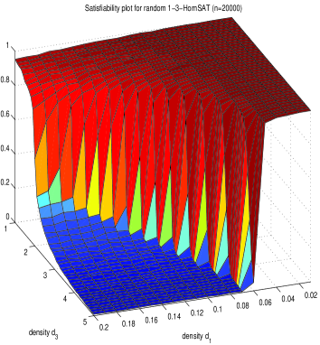
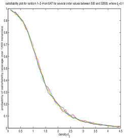
Motivated by the connection between the automata emptiness problem and Horn satisfiability, Demopoulos and Vardi [14] studied the satisfiability of two types of fixed-clause-length random Horn-SAT formulae. They considered 1-2-Horn-SAT, where formulae consist of clauses of length one and two only, and 1-3-Horn-SAT, where formulae consist of clauses of length one and three only. These two classes can be viewed as the Horn analogue of 2-SAT and 3-SAT. For 1-2-Horn-SAT, they showed experimentally that there is a coarse transition (see Figure 4), which can be explained and analyzed in terms of random digraph connectivity [22]. The situation for of 1-3-Horn-SAT is less clear cut. On one hand, recent results on random undirected hypergraphs [13] fit the experimental data of [14] quite well. On the other, a scaling analysis of the data suggested that transition between the mostly-satisfiable and mostly-unsatisfiable regions (the “waterfall” in Figure 1) is steep but continuous, rather than a step function. It was therefore not clear if the model exhibits a phase transition, in spite of experimental data for instances with tens of thousands of variables.

In this paper we generalize the fixed-clause-length model of [14] and offer a complete analysis of the probability of satisfiability in this model. For a finite $k>0$ and a vector ${\bf d}$ of $k$ nonnegative real numbers ${d_{1},d_{2},\ldots,d_{k}}$, $d_{1}<1$, let the random Horn-SAT formula $H^{k}_{n,{\bf d}}$ be the conjunction of

• a single negative literal $\overline{x}_{1}$,

• $d_{1}n$ positive literals chosen uniformly without replacement from $x_{2},\ldots,x_{n}$, and

• for each $2\leq j\leq k$, $d_{j}n$ clauses chosen uniformly from the $j{n\choose j}$ possible Horn clauses with $j$ variables where one literal is positive.

Thus, the classes studied in [14] are $H^{2}_{n,d_{1},d_{2}}$ and $H^{3}_{n,d_{1},0,d_{3}}$ respectively.

Figure 1: Satisfiability probability of a random 1-3-Horn formula of size 20000. Left, the experimental results of [14]; right, our analytic results.

With this model in hand, we settle the question of sharp thresholds for 1-3-Horn-SAT. In particular, we show that there are sharp thresholds in some regions of the $(d_{1},d_{3})$ plane in the probability of satisfiability, although not from $1$ to $0$. We start with the following general result for the $H^{k}_{n,{\bf d}}$ model.

Theorem 1.1

Let $t_{0}$ be the smallest positive root of the equation

$$\ln\frac{1-t}{1-d_{1}}+\sum_{j=2}^{k}d_{j}t^{j-1}=0\enspace.$$ (1)

Call $t_{0}$ simple if it is not a double root of (1), i.e., if the derivative of the left-hand-side of (1) with respect to $t$ is nonzero at $t_{0}$. If $t_{0}$ is simple, the probability that a random formula from $H^{k}_{n,{\bf d}}$ is satisfiable in the limit $n\to\infty$ is

$$\Phi({\bf d}):=\lim_{n\rightarrow\infty}\Pr[H^{k}_{n,{\bf d}}\mbox{ is satisfiable}]=\frac{1-t_{0}}{1-d_{1}}\enspace.$$ (2)

Specializing this result to the case $k=2$ yields an exact formula that matches the experimental results in [14]:

Proposition 1.2

The probability that a random formula from $H^{2}_{n,d_{1},d_{2}}$ is satisfiable in the limit $n\to\infty$ is

$$\Phi(d_{1},d_{2}):=\lim_{n\rightarrow\infty}\Pr[H^{2}_{n,d_{1},d_{2}}\mbox{ is satisfiable}]=-\frac{W\bigl{(}-(1-d_{1})d_{2}e^{-d_{2}}\bigr{)}}{(1-d_{1})d_{2}}\enspace.$$ (3)

Here $W(\cdot)$ is Lambert’s function, defined as the principal root of the equation $W(x)e^{W(x)}=x$.

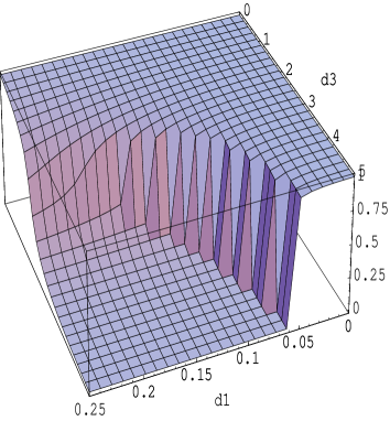
For the case $k=3$ and $d_{2}=0$, we do not have a closed-form expression for the probability of satisfiability, though numerically Figure 1 shows a very good fit to the experimental results of [14]. In addition, we find an interesting phase transition behavior in the $(d_{1},d_{3})$ plane, described by the following proposition.

Proposition 1.3

The probability of satisfiability $\Phi(d_{1},d_{3})$ that a random formula from $H^{3}_{n,d_{1},0,d_{3}}$ is satisfiable is continuous for $d_{3}<2$ and discontinuous for $d_{3}>2$. Its discontinuities are given by a curve $\Gamma$ in the $(d_{1},d_{3})$ plane described by the equation

$$d_{1}=1-\frac{\exp\left(\frac{1}{4}\left(\sqrt{d_{3}}-\sqrt{d_{3}-2}\right)^{2}\right)}{d_{3}-\sqrt{d_{3}(d_{3}-2)}}\enspace.$$ (4)

This curve consists of the points $(d_{1},d_{3})$ at which $t_{0}$ is a double root of (1), and ends at the critical point

$$(1-\sqrt{{\rm e}}/2,2)=(0.1756...,2)\enspace.$$

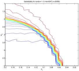
The curve $\Gamma$ of discontinuities described in Proposition 1.3 can be seen in the right part of Figure 1. The drop at the “waterfall” decreases as we approach the critical point $(0.1756...,2)$, where the probability of satisfiability becomes continuous (although its derivatives at that point are infinite). We can also see this in Figure 2, which shows a contour plot; the contours are bunched at the discontinuity, and “fan out” at the critical point. In both cases our calculates closely match the experimental results of [14].

Figure 2: Contour plots. Left, the experimental results of [14]. Right, our analytical results.

In statistical physics, we would say that $\Gamma$ is a curve of first-order transitions, in which the order parameter is discontinuous, ending in a second-order transition at the tip of the curve, at which the order parameter is continuous, but has a discontinuous derivative (see e.g. [5]). A similar transition takes place in the Ising model, where the two parameters are the temperature $T$ and the external field $H$; the magnetization is discontinuous at the line $H=0$ for $T<T_{c}$ where $T_{c}$ is the transition temperature, but there is a second-order transition at $(T_{c},0)$ and the magnetization is continuous for $T\geq T_{c}$.

To our knowledge, this is the first time that a continuous-discontinuous transition of this type has been established rigorously in a model of random constraint satisfaction problems. We note that a similar phenomenon is believed to take place for $(2+p)$-SAT model at the triple point $p=2/5$; here the order parameter is the size of the backbone, i.e., the number of variables that take fixed values in every truth assignment [3, 27]. Indeed, in our model the probability of satisfiability is closely related to the size of the backbone, as we see below.

2 Horn-SAT and Automata

Our main motivation for studying the satisfiability of Horn formulae is the unusually rich type of phase transition described above, and the fact that its tractability allows us to perform experiments on formulae of very large size. However, the original motivation of [14] that led to the present work is the fact that Horn formulae can be used to describe finite automata on words and trees.

A finite automaton $A$ is a 5-tuple $A=(S,\Sigma,\delta,s,F)$, where $S$ is a finite set of states, $\Sigma$ is an alphabet, $s$ is a starting state, $F\subseteq S$ is the set of final (accepting) states and $\delta$ is a transition relation. In a word automaton, $\delta$ is a function from $S\times\Sigma$ to $2^{S}$, while in a binary-tree automaton $\delta$ is a function from $S\times\Sigma$ to $2^{S\times S}$. Intuitively, for word automata $\delta$ provides a set of successor states, while for binary-tree automata $\delta$ provides a set of successor state pairs. A run of an automaton on a word $a=a_{1}a_{2}\cdots a_{n}$ is a sequence of states $s_{0}s_{1}\cdots s_{n}$ such that $s_{0}=s$ and $(s_{i-1},a_{i},s_{i})\in\delta$. A run is succesful if $s_{n}\in F$: in this case we say that $A$ accepts the word $a$. A run of an automaton on a binary tree $t$ labeled with letters from $\Sigma$ is a binary tree $r$ labeled with states from $S$ such that root$(r)=s$ and for a node $i$ of $t$, $(r(i),t(i),r(\mbox{left-child-of-}i),r(\mbox{right-child-of-}i))\in\delta$. Thus, each pair in $\delta(r(i),t(i))$ is a possible labeling of the children of $i$. A run is succesful if for all leaves $l$ of $r$, $r(l)\in F$: in this case we say that $A$ accepts the tree $t$. The language $L(A)$ of a word automaton $A$ is the set of all words $a$ for which there is a successful run of $A$ on $a$. Likewise, the language $L(A)$ of a tree automaton $A$ is the set of all trees $t$ for which there is a successful run of $A$ on $t$. An important question in automata theory, which is also of great practical importance in the field of formal verification [30, 31], is: given an automaton $A$, is $L(A)$ non-empty? We now show how the problem of non-emptiness of automata languages translates to Horn satisfiability. Thus, getting a better understanding of the satisfiability of Horn formulae would tell us about the expected answer to automata nonemptiness problems.

Consider first a word automaton $A=(S,\Sigma,\delta,s_{0},F)$. Construct a Horn formula $\phi_{A}$ over the set $S$ of variables as follows: create a clause $(\bar{s_{0}})$, for each $s_{i}\in F$ create a clause $(s_{i})$, for each element $(s_{i},a,s_{j})$ of $\delta$ create a clause $(\bar{s_{j}},s_{i})$, where $(s_{i},\cdots,s_{k})$ represents the clause $s_{i}\vee\cdots\vee s_{k}$ and $\bar{s_{j}}$ is the negation of $s_{j}$. Similarly to the word automata case, we can show how to construct a Horn formula from a binary-tree automaton. Let $A=(S,\Sigma,\delta,s_{0},F)$ be a binary-tree automaton. Then we can construct a Horn formula $\phi_{A}$ using the construction above with the only difference that since $\delta$ in this case is a function from $S\times\{\alpha\}$ to $S\times S$, for each element $(s_{i},\alpha,s_{j},s_{k})$ of $\delta$ we create a clause $(\bar{s_{j}},\bar{s_{k}},s_{i})$.

Proposition 2.1

[14] Let $A$ be a word or binary tree automaton and $\phi_{A}$ the Horn formula constructed as described above. Then $L(A)$ is non-empty if and only if $\phi_{A}$ is unsatisfiable.

3 Main Result

Algorithm ${\rm PUR}$: 1. while ($\phi$ contains positive unit clauses) 2. choose a random positive unit clause $x$ 3. remove all other clauses in which $x$ occurs positively in $\phi$ 4. shorten all clauses in which $x$ appears negatively 5. label $x$ as “implied” and call the algorithm recursively. 6. if no contradictory clause was created 7. accept $\phi$ 8. else 9. reject $\phi$.

Figure 3: Positive Unit Resolution.

Consider the positive unit resolution algorithm ${\rm PUR}$ applied to a random formula $\phi$ (Figure 3). The proof of Theorem 1.1 follows immediately from the following theorem, which establishes the size of the backbone of the formula with the single negative literal $\overline{x}_{1}$ removed: that is, the set of positive literals implied by the positive unit clauses and the clauses of length greater than $1$. Then $\phi$ is satisfiable as long as $x_{1}$ is not in this backbone.

Lemma 3.1

Let $\phi$ be a random Horn-SAT formula $H^{k}_{n,{\bf d}}$ with $d_{1}>0$. Denote by $t_{0}$ the smallest positive root of Equation (1), and suppose that $t_{0}$ is simple. Then, for any $\epsilon>0$, the number $N_{{\bf d},n}$ of implied positive literals, including the $d_{1}n$ initially positive literals, satisfies w.h.p. the inequality

$$(t_{0}-\epsilon)\cdot n<N_{{\bf d},n}<(t_{0}+\epsilon)\cdot n,$$ (5)

• First, we give a heuristic argument, analogous to the branching process argument for the size of the giant component in a random graph. The number $m$ of clauses of length $j$ with a given literal $x$ as their implicate (i.e., in which $x$ appears positively) is Poisson-distributed with mean $d_{j}$. If any of these clauses have the property that all their literals whose negations appear are implied, then $x$ is implied as well. In addition, $x$ is implied if it is one of the $d_{1}n$ initially positive literals. Therefore, the probability that $x$ is not implied is the probability that it is not one of the initially positive literals, and that, for all $j$, for all $m$ clauses $c$ of length $j$ with $x$ as their implicate, at least one of the $j-1$ literals whose negations appear in $c$ is not implied. Assuming all these events are independent, if $t$ is the fraction of literals that are implied, we have

  $$1-t =(1-d_{1})\prod_{j=2}^{k}\left(\sum_{m=0}^{\infty}\frac{{\rm e}^{-d_{j}}d_{j}^{m}}{m!}(1-t^{j-1})^{m}\right)$$

  $$=(1-d_{1})\prod_{j=2}^{k}\exp(-d_{j}t^{j-1}))=(1-d_{1})\,\exp\left(-\sum_{j=2}^{k}d_{j}t^{j-1}\right)$$

  yielding Equation (1).

  To make this rigorous, we use a standard technique for proving results about threshold properties: analysis of algorithms via differential equations [32] (see [1] for a review). We analyze the while loop of ${\rm PUR}$ shown in Figure 3; specifically, we view ${\rm PUR}$ as working in stages, indexed by the number of literals that are labeled “implied.” After $T$ steps of this process, $T$ variables are labeled as implied. At each stage the resulting formula consists of a set of Horn clauses of length $j$ for $1\leq j\leq k$ on the $n-T$ unlabeled variables. Let the number of distinct clauses of length $j$ in this formula be $S_{j}(T)$; we rely on the fact that, at each stage $T$, conditioned on the values of $S_{j}(T)$ the formula is uniformly random. This follows from an easy induction argument which is standard for problems of this type (see e.g. [21]).

Now, the variables appearing in the clauses present at stage $T$ are chosen uniformly from the $n-T$ remaining variables, so the probability that the chosen variable $x$ appears in a given clause of length $j$ is $j/(n-T)$, and the probability that a given clause of length $j+1$ is shortened to one of length $j$ (as opposed to removed) is $j/(n-T)$. A newly shortened clause is distinct from all the others with probability $1-o(1)$ unless $j=1$, in which case it is distinct with probability $(n-T-S_{1})/(n-T)$. Finally, each stage labels the variable in one of the $S_{1}(T)$ unit clauses as implied. Thus the expected effect of each step is

$${\rm E}[S_{j}(T+1)] = S_{j}(T)+j\frac{S_{j+1}(T)-S_{j}(T)}{n-T}+o(1)\quad\mbox{for all }2\leq j\leq k$$

$${\rm E}[S_{1}(T+1)] = S_{1}(T)+\left(\frac{n-T-S_{1}}{n-T}\right)\left(\frac{S_{2}(T)}{n-T}\right)-1+o(1)$$

Setting $T=t\cdot n$ and $S_{j}(T)=s_{j}(t)\cdot n$, we rescale this to form a system of differential equations:

$$\frac{{\rm d}s_{j}}{{\rm d}t} = j\,\frac{s_{j+1}(t)-s_{j}(t)}{1-t}\quad\mbox{for all }2\leq j\leq k$$

$$\frac{{\rm d}s_{1}}{{\rm d}t} = \left(\frac{1-t-s_{1}(t)}{1-t}\right)\left(\frac{s_{2}(t)}{1-t}\right)-1\enspace.$$ (6)

Then Wormald’s Theorem tells us that, for any constant $\delta>0$, for all $t$ such that $s_{1}>\delta$, w.h.p. we have $S_{j}(t\cdot n)=s_{j}(t)\cdot n+o(n)$ where $s_{j}(t)$ is the solution to the system (6). With the initial conditions $s_{j}(0)=d_{j}$ for $1\leq j\leq k$, a little work shows that this solution is

$$s_{j}(t) = (1-t)^{j}\,\sum_{\ell=j}^{k}{\ell-1\choose j-1}\,d_{\ell}t^{\ell-j}\quad\mbox{for all }2\leq j\leq k$$

$$s_{1}(t) = 1-t-(1-d_{1})\exp\left(-\sum_{j=2}^{k}d_{j}t^{j-1}\right)\enspace.$$ (7)

Note that $s_{1}(t)$ is continuous, $s_{1}(0)=d_{1}>0$, and $s_{1}(1)<0$ since $d_{1}<1$. Thus $s_{1}(t)$ has at least one root in the interval $(0,1)$. Since ${\rm PUR}$ halts when there are no unit clauses, i.e., when $S_{1}(T)=0$, we expect the stage at which it halts. Thus the number of implied positive literals, to be $T=t_{0}n+o(n)$ where $t_{0}$ is the smallest positive root of $s_{1}(t)=0$, or equivalently, dividing by $1-d_{1}$ and taking the logarithm, of Equation (1).

However, the conditions of Wormald’s theorem do not allow us to run the differential equations all the way up to stage $t_{0}n$. We therefore choose small constants $\epsilon,\delta>0$ such that $s_{1}(t_{0}-\epsilon)=\delta$ and run the algorithm until stage $(t_{0}-\epsilon)n$. At this point $(t_{0}-\epsilon)n$ literals are already implied, proving the lower bound of (5).

To prove the upper bound of (5), recall that by assumption $t_{0}$ is a simple root of (1), i.e., the second derivative of the left-hand size of (1) with respect to $t$ is nonzero at $t_{0}$. It is easy to see that this is equivalent to ${\rm d}s_{1}/{\rm d}t<0$ at $t_{0}$. Since ${\rm d}s_{1}/{\rm d}t$ is analytic, there is a constant $c>0$ such that ${\rm d}s_{1}/{\rm d}t<0$ for all $t_{0}-c\leq t\leq t_{0}+c$. Set $\epsilon<c$; the number of literals implied during these stages is bounded above by a subcritical branching process whose initial population is w.h.p. $\delta n+o(n)$, and by standard arguments we can bound its total progeny to be $\epsilon^{\prime}n$ for any $\epsilon^{\prime}>0$ by taking $\delta$ small enough.      

It is easy to see that the backbone of implied positive literals is a uniformly random subset of $\{x_{1},\ldots,x_{n}\}$ of size $N_{{\bf d},n}$. Since $x_{1}$ is guaranteed to not be among the $d_{1}n$ initially positive literals, the probability that $x_{1}$ is not in this backbone is

$$\frac{n-N_{{\bf d},n}}{(1-d_{1})\cdot n}.$$

By completeness of positive unit resolution for Horn satisfiability, this is precisely the probability that the $\phi$ is satisfiable. Applying Lemma 3.1 and taking $\epsilon\rightarrow 0$ proves equation (2) and completes the proof of Theorem 1.1.

We make several observations. First, if we set $k=2$ and take the limit $d_{1}\to 0$, Theorem 3.1 recovers Karp’s result  [22] on the size of the reachable component of a random directed graph with mean out-degree $d=d_{2}$, the root of $\ln(1-t)+dt=0$.

Secondly, as we will see below, the condition that $t_{0}$ is simple is essential. Indeed, for the 1-3-Horn-SAT model studied in [14], the curve $\Gamma$ of discontinuities, where the probability of satisfiability drops in the “waterfall” of Figure 1, consists exactly of those $(d_{1},d_{3})$ where $t_{0}$ is a double root, which implies ${\rm d}s_{1}/{\rm d}t=0$ at $t_{0}$.

Finally, we note that Theorem 3.1 is very similar to Darling and Norris’s work on identifiability in random undirected hypergraphs [13], where the number of hyperedges of length $j$ is Poisson-distributed with mean $\beta_{j}$. Their result reads

$$\ln(1-t)+\sum_{j=1}^{k}j\beta_{j}t^{j-1}=0\enspace.$$

We can make this match (1) as follows. First, since each hyperedge of length $j$ corresponds to $j$ Horn clauses, we set $d_{j}=j\beta_{j}$ for all $j\geq 2$. Then, since edges are chosen with replacement in their model, the expected number of distinct clauses of length $1$ (i.e., positive literals) is $d_{1}n$ where $d_{1}=1-{\rm e}^{-\beta_{1}}$.

4 Application to $H_{n,{\bf d}}^{2}$

For $H_{n,{\bf d}}^{2}$, Equation (1) can rewritten as $1-t=(1-d_{1})\cdot e^{-d_{2}\cdot t}$. Denoting $y=d_{2}(t-1)$, this implies

$$y\cdot e^{y}=d_{2}(t-1)\cdot e^{d_{2}\cdot(t-1)}=-d_{2}(1-d_{1})\cdot e^{-d_{2}\cdot t}\cdot e^{d_{2}\cdot(t-1)}=-(1-d_{1})d_{2}e^{-d_{2}}.$$

Solving this yields

$$t_{0}=1+\frac{1}{d_{2}}W\bigl{(}-(1-d_{1})d_{2}{\rm e}^{-d_{2}}\bigr{)}$$

and substituting this into (2) proves Equation (3) and Proposition 1.2. In Figure 4 we plot the probability of satisfiability $\Phi(d_{1},d_{2})$ as a function of $d_{2}$ for $d_{1}=0.1$ and compare it with the experimental results of [14]; the agreement is excellent.

Figure 4: The probability of satisfiability for 1-2-Horn formulae as a function of $d_{2}$, where $d_{1}=0.1$. Left, our analytic results; right, the experimental data of [14].

5 A continuous-discontinuous phase transition for $H_{n,d_{1},0,d_{3}}^{3}$

For the random model $H_{n,d_{1},0,d_{3}}^{3}$ studied in [14], an analytic solution analogous to (3) does not seem to exist. Let us, however, rewrite (1) as

$$1-t=f(t):=(1-d_{1}){\rm e}^{-d_{3}t^{2}}\enspace.$$ (8)

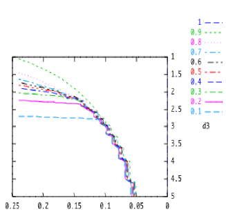
We claim that for some values of $d_{1}$ and $d_{3}$ there is a phase transition in the roots of (8). For instance, consider the plot of $f(t)$ shown in Figure 5 for $d_{1}=0.1$ and $d_{3}=3$. Here $f(t)$ is tangent to $1-t$, so there is a bifurcation as we vary either parameter; for $d_{3}=2.9$, for instance, $f(t)$ crosses $1-t$ three times and there is a root of (8) at $t=0.185$, but for $d_{3}=3.1$ the unique root is at $t=0.943$. This causes the probability of satisfiability to jump discontinuously but from $0.905$ to $0.064$. The set of pairs $(d_{1},d_{3})$ for which $f(t)$ is tangent to $1-t$ is exactly the curve $\Gamma$ on which the smallest positive root $t_{0}$ of (1) or (8) is a double root, giving the “waterfall” of Figure 1.

Figure 5: Left, the function $f(t)$ of (8) when $d_{1}=0.1$ and $d_{3}=3$. Right, the probability of satisfiability $\Phi(d_{1},d_{3})$ with $d_{1}$ equal to $0.15$ (continuous), $0.1756$ (critical), and $0.2$ (discontinuous).

To find where this transition takes place, we set $f^{\prime}=-1$, yielding $f(t)=1/(2d_{3}t)$. Setting this to $1-t$ and solving for $t$ gives

$$d_{1}=1-\frac{{\rm e}^{d_{3}t^{2}}}{2d_{3}t}$$ (9)

where

$$t=\frac{1}{2}\left(1-\sqrt{1-\frac{2}{d_{3}}}\right)$$ (10)

Substituting (10) in (9) and simplifying gives (4), proving Proposition 1.3.

The fact that $d_{1}$ is only real for $d_{3}\geq 2$ explains why $\Gamma$ ends at $d_{3}=2$. At this extreme case we have

$$d_{1}=1-\frac{\sqrt{{\rm e}}}{2}\approx 0.1756\;\mbox{ and }\;\frac{\partial d_{1}}{\partial d_{3}}=-\frac{\sqrt{{\rm e}}}{8}\enspace.$$

What happens for $d_{3}<2$? In this case, there are no real $t$ for which $f^{\prime}(t)=-1$, so the kind of tangency displayed in Figure 5 cannot happen. In that case, (8) (and equivalently (1)) has a unique solution $t$, which varies continuously with $d_{1}$ and $d_{3}$, and therefore the probability of satisfiability $\Phi(d_{1},d_{3})$ is continuous as well. To illustrate this, in the right part of Figure 5 we plot $\Phi(d_{1},d_{3})$ as a function of $d_{3}$ with three values of $d_{1}$. For $d_{1}=0.15$, $\Phi$ is continuous; for $d_{1}=0.2$, it is discontinuous; and for $d_{1}=0.1756...$, the critical value at the second-order transition, it is continuous but has an infinite derivative at $d_{3}=2$.

References

- [1] D. Achlioptas. Lower Bounds for Random 3-SAT via Differential Equations. Theoretical Computer Science 265 (1-2), 159–185, 2001.
- [2] D. Achlioptas, A. Chtcherba, G. Istrate, and C. Moore. The phase transition in 1-in- SAT and NAE 3-SAT. In Proc. 12th ACM-SIAM Symp. on Discrete Algorithms, 721–722, 2001.
- [3] D. Achlioptas, L.M. Kirousis, E. Kranakis, and D. Krizanc. Rigorous results for random -SAT. Theor. Comput. Sci. 265(1-2): 109-129 (2001).
- [4] T. Bench-Capon and P. Dunne. A sharp threshold for the phase transition of a restricted satisfiability problem for Horn clauses. Journal of Logic and Algebraic Programming, 47(1):1–14, 2001.
- [5] J. J. Binney, N. J. Dowrick, A. J. Fisher and M. E. J. Newman. The Theory of Critical Phenomena. Oxford University Press (1992).
- [6] B. Bollobás. Random Graphs. Academic Press, 1985.
- [7] S. Cocco, O. Dubois, J. Mandler, and R. Monasson. Rigorous decimation-based construction of ground pure states for spin glass models on random lattices. Phys. Rev. Lett., 90, 2003.
- [8] V. Chvátal and B. Reed. Mick gets some (the odds are on his side). In Proc. 33rd IEEE Symp. on Foundations of Computer Science, IEEE Comput. Soc. Press, 620–627, 1992.
- [9] J. M. Crawford and L. D. Auton. Experimental results on the crossover point in random 3-SAT. Artificial Intelligence, 81(1-2):31–57, 1996.
- [10] W. F. Dowling and J. H. Gallier. Linear-time algorithms for testing the satisfiability of propositional Horn formulae. Logic Programming. (USA) ISSN: 0743-1066, 1(3):267–284, 1984.
- [11] O. Dubois, Y. Boufkhad, and J. Mandler. Typical random 3-SAT formulae and the satisfiability theshold. In Proc. 11th ACM-SIAM Symp. on Discrete Algorithms, 126–127, 2000.
- [12] O. Dubois and J. Mandler. The 3-XORSAT threshold. In Proc. 43rd IEEE Symp. on Foundations of Computer Science, 769–778, 2002.
- [13] R. Darling and J.R. Norris. Structure of large random hypergraphs. Annals of Applied Probability, 15(1A), 2005.
- [14] D. Demopoulos and M. Vardi. The phase transition in random 1-3 Hornsat problems. In A. Percus, G. Istrate, and C. Moore, editors, Computational Complexity and Statistical Physics, Santa Fe Institute Lectures in the Sciences of Complexity. Oxford University Press, 2005. Available at http://www.cs.rice.edu/∼vardi/papers/.
- [15] P. Erdös and A. Rényi. On the evolution of random graphs. Publications of the Mathematical Institute of the Hungarian Academy of Science, 5:17–61, 1960.
- [16] E. Friedgut. Necessary and sufficient conditions for sharp threshold of graph properties and the -SAT problem. J. Amer. Math. Soc., 12:1917–1054, 1999.
- [17] A. Goerdt. A threshold for unsatisfiability. J. Comput. System Sci., 53(3):469–486, 1996.
- [18] M. Hajiaghayi and G.B. Sorkin. The satisfiability threshold for random 3-SAT is at least 3.52. IBM Technical Report , 2003.
- [19] T. Hogg and C. P. Williams. The hardest constraint problems: A double phase transition. Artificial Intelligence, 69(1-2):359–377, 1994.
- [20] G. Istrate. The phase transition in random Horn satisfiability and its algorithmic implications. Random Structures and Algorithms, 4:483–506, 2002.
- [21] G. Istrate. On the satisfiability of random -Horn formulae. In P. Winkler and J. Nesetril, editors, Graphs, Morphisms and Statistical Physics, volume 64 of AMS-DIMACS Series in Discrete Mathematics and Theoretical Computer Science, 113–136, 2004.
- [22] R. Karp. The transitive closure of a random digraph. Random Structures and Algorithms, 1:73–93, 1990.
- [23] A. Kaporis, L. M. Kirousis, and E. Lalas. Selecting complementary pairs of literals. In Proceedings of LICS’03 Workshop on Typical Case Complexity and Phase Transitions, June 2003.
- [24] J. A. Makowsky. Why Horn formulae matter in Computer Science: Initial structures and generic examples. JCSS, 34(2-3):266–292, 1987.
- [25] M. Mézard and R. Zecchina. Random k-satisfiability problem: from an analytic solution to an efficient algorithm. Phys. Rev. E, 66:056126, 2002.
- [26] M. Mézard, G. Parisi, and R. Zecchina. Analytic and algorithmic solution of random satisfiability problems. Science, 297:812–815, 2002.
- [27] R. Monasson, R. Zecchina, S. Kirkpatrick, B. Selman, and L. Troyansky. -SAT: Relation of typical-case complexity to the nature of the phase transition. Random Structures and Algorithms, 15(3–4):414–435, 1999.
- [28] B. Selman, D. G. Mitchell, and H. J. Levesque. Generating hard satisfiability problems. Artificial Intelligence, 81(1-2):17–29, 1996.
- [29] B. Selman and S. Kirkpatrick. Critical behavior in the computational cost of satisfiability testing. Artificial Intelligence, 81(1-2):273–295, 1996.
- [30] M.Y. Vardi and P. Wolper. Automata-Theoretic Techniques for Modal Logics of Programs J. Computer and System Science 32:2(1986), 181–221, 1986.
- [31] M.Y. Vardi and P. Wolper. An automata-theoretic approach to automatic program verification (preliminary report). In Proc. 1st IEEE Symp. on Logic in Computer Science, 332–344, 1986.
- [32] N. Wormald. Differential equations for random processes and random graphs. Annals of Applied Probability, 5(4):1217–1235, 1995.