Dessins d’Enfants and Hypersurfaces with
Many $A_{j}$-Singularities

Abstract.

We show the existence of surfaces of degree $d$ in ${\mathds{P}}^{3}({\mathds{C}})$ with approximately ${3j+2\over 6j(j+1)}d^{3}$ singularities of type $A_{j},2\leq j\leq d-1$. The result is based on Chmutov’s construction of nodal surfaces. For the proof we use plane trees related to the theory of Dessins d’Enfants.

Our examples improve the previously known lower bounds for the maximum number $\mu_{A_{j}}(d)$ of $A_{j}$-singularities on a surface of degree $d$ in most cases. We also give a generalization to higher dimensions which leads to new lower bounds even in the case of nodal hypersurfaces in ${\mathds{P}}^{n},n\geq 5$.

To conclude, we work out in detail a classical idea of B. Segre which leads to some interesting examples, e.g. to a sextic with $36$ cusps.

1. Introduction

All possible configurations of singularities on a surface of degree $3$ in ${\mathds{P}}^{3}:={\mathds{P}}^{3}({\mathds{C}})$ are known since Schläfli’s work [25] in the $19^{\textup{th}}$ century, see [14] and [18] for explicit equations and illustrating pictures. In the case of degree $4$, the classification was completed recently by Yang [29] using computers.

Much less is known for higher degrees, even when restricting to a particular type of singularity. E.g., the maximum number of $A_{1}$-singularities on a surface of degree $d$ is only known for $d\leq 6$. We recently improved the case $d=7$ using computer algebra and geometry over prime fields [19]. The best lower bounds for surfaces of large degree $d$ with $A_{1}$-singularities are given by Chmutov’s construction [9].

For higher singularities — e.g., singularities of type $A_{j}$ which are locally equivalent to $x^{j+1}+y^{2}+z^{2}$ — the situation is even more difficult. We denote by $\mu_{A_{j}}(d)$ the maximum number of singularities of type $A_{j}$ a surface of degree $d$ in ${\mathds{P}}^{3}$ can have. Barth [5] constructed a quintic with $15$ singularities of type $A_{2}$ (also called (ordinary) cusps), and the author constructed a sextic with $35$ such singularities [20] using computer algebra in characteristic zero which showed $\mu_{A_{2}}(6)\geq 35$. The detailed study of a generalization of an idea of B. Segre [26] which we give in the appendix leads to: $\mu_{A_{2}}(6)\geq 36$ (see equations (11) and (12), and corollary 12). Recently, Barth and others considered the codes connected to surfaces with three-divisible cusps in analogy to the codes related to even sets of nodes, see [4, 6, 23].

In general, the best lower bounds for the $\mu_{A_{j}}(d)$ known up to now are given by a direct generalization of an idea already used by Rohn in the $19^{\textup{\tiny th}}$ century [24, p. 33]: $\mu_{A_{j}}(d)\geq{1\over 2}d(d-1)\lfloor{d\over j+1}\rfloor$ for $d\geq 2(j+1)$ (see, e.g., [6] and [20] for applications of this). For many degrees, one can also use the already mentioned generalization of B. Segre’s construction [26] which is usually better than Rohn’s if it can be applied.

In the main part of the article we describe a variant of Chmutov’s construction [9] which leads to the lower bound (corollary 9):

(1) $$\mu_{A_{j}}(d)\ \gtrapprox\ {3j+2\over 6j(j+1)}d^{3}.$$

To our knowledge, this gives asymptotically the best known bounds for any $j\geq 2$. The construction reaches more than $\approx 75\%$ of the theoretical upper bound in all cases. We compute this upper bound in section 7. Table 1 gives an overview of our results for low $j$, see also corollaries 9 and 10. We describe a generalization of our construction to higher dimensions in section 8. This leads to new lower bounds even in the case of nodal hypersurfaces.

	$3$	$4$	$5$	$6$	$7$	$8$	$9$	$10$	$11$	$12$	$d$
$1$											$\approx\ \,\begin{tabular}[]{@{}c@{}}{\rule{0.0pt}{16.00008pt}\begin{picture}(347.0,215.0)(-41.0,616.0){\color[rgb]{0,0,0}\put(1.0,659.0){\line(2,1){270.0}} }\put(122.0,616.0){\makebox(0.0,0.0)[lb]{\smash{{{\color[rgb]{0,0,0}4/9}}}}} \put(143.0,756.0){\makebox(0.0,0.0)[rb]{\smash{{{\color[rgb]{0,0,0}5/12}}}}} \end{picture}}\end{tabular}\cdot d^{3}$
$2$											$\approx\,\begin{tabular}[]{@{}c@{}}{\rule{0.0pt}{16.00008pt}\begin{picture}(347.0,215.0)(-41.0,616.0){\color[rgb]{0,0,0}\put(1.0,659.0){\line(2,1){270.0}} }\put(122.0,616.0){\makebox(0.0,0.0)[lb]{\smash{{{\color[rgb]{0,0,0}1/4}}}}} \put(143.0,756.0){\makebox(0.0,0.0)[rb]{\smash{{{\color[rgb]{0,0,0}{2/9}}}}}} \end{picture}}\end{tabular}\cdot d^{3}$
$3$											$\approx\ \ \;\begin{tabular}[]{@{}c@{}}{\rule{0.0pt}{16.00008pt}\begin{picture}(347.0,215.0)(-41.0,616.0){\color[rgb]{0,0,0}\put(1.0,659.0){\line(2,1){270.0}} }\put(122.0,616.0){\makebox(0.0,0.0)[lb]{\smash{{{\color[rgb]{0,0,0}8/45}}}}} \put(143.0,756.0){\makebox(0.0,0.0)[rb]{\smash{{{\color[rgb]{0,0,0}{11/72}}}}}} \end{picture}}\end{tabular}\ \cdot d^{3}$
$4$											$\approx\ \,\begin{tabular}[]{@{}c@{}}{\rule{0.0pt}{16.00008pt}\begin{picture}(347.0,215.0)(-41.0,616.0){\color[rgb]{0,0,0}\put(1.0,659.0){\line(2,1){270.0}} }\put(122.0,616.0){\makebox(0.0,0.0)[lb]{\smash{{{\color[rgb]{0,0,0}5/36}}}}} \put(143.0,756.0){\makebox(0.0,0.0)[rb]{\smash{{{\color[rgb]{0,0,0}{7/60}}}}}} \end{picture}}\end{tabular}\ \cdot d^{3}$

Table 1. Known upper and lower bounds for the maximum number $\mu_{A_{j}}(d)$ of singularities of type $A_{j},\ j=1,2,3,4,$ on a surface of degree $d$ in ${\mathds{P}}^{3}$. For $j\geq 2$ and $d\geq 5$, the lower bounds are attained by our examples or by the generalization of B. Segre’s idea which we work out in the appendix.

I thank D. van Straten for all his motivation, many valuable discussions, and for introducing me to the theory of Dessins d’Enfants.

2. Chmutov’s Idea

We start with some notation: A point $z_{0}\in{\mathds{C}}$ is a critical point of multiplicity $j\in{\mathds{N}}$ of a polynomial $g\in{\mathds{C}}[z]$ in one variable if the first $j$ derivatives of $g$ vanish at $z_{0}$: $g^{(1)}(z_{0})=\cdots=g^{(j)}(z_{0})=0$. The number $g(z_{0})$ is called the critical value of $z_{0}$. A critical point of multiplicity $j,j>1,$ is called a degenerate critical point.

In [9], Chmutov uses the following idea:

• Let $P_{d}(x,y)\in{\mathds{C}}[x,y]$ be a polynomial of degree $d$ with few different critical values, all of which are non-degenerate. By a coordinate change, we may assume that the two critical values which occur most often are $0$ and $-1$. We assume that they occur $\nu(0)$ and $\nu(-1)$ times, and that $\nu(0)>\nu(-1)$.

• Let $T_{d}(z)\in{\mathds{R}}[z]$ be the Chebychev polynomial of degree $d$ with critical values $-1$ and $+1$, where $-1$ occurs $\lfloor{d\over 2}\rfloor$ times and $+1$ occurs $\lfloor{d-1\over 2}\rfloor$ times.

• It is easy to see that the projective surface given by the affine equation

  (2) $$P_{d}(x,y)+\frac{1}{2}(T_{d}(z)+1)=0$$

  has $\nu(0)\cdot\lfloor{d\over 2}\rfloor+\nu(-1)\cdot\lfloor{d-1\over 2}\rfloor$ nodes.

Chmutov uses for $P_{d}(x,y)$ the so-called folding polynomials $F^{A_{2}}_{d}$ associated to the root system $A_{2}$ (see [28]):

(3) $$F^{A_{2}}_{d}(x,y):=2+\det\left(\begin{array}[]{c@{\,}c@{\,}c@{\,}c@{\,}c@{\,}c@{\,}c}\rule{0.0pt}{12.59996pt}x&1&0&\cdots&\cdots&\cdots&0\\[-5.40005pt] \rule{0.0pt}{12.59996pt}2y&x&\ddots&\ddots&&&\vdots\\[-5.40005pt] \rule{0.0pt}{12.59996pt}3&y&\ddots&\ddots&\ddots&&\vdots\\[-5.40005pt] \rule{0.0pt}{12.59996pt}0&1&\ddots&\ddots&\ddots&\ddots&\vdots\\[-5.40005pt] \rule{0.0pt}{12.59996pt}\vdots&\ddots&\ddots&\ddots&\ddots&\ddots&0\\[-5.40005pt] \rule{0.0pt}{12.59996pt}\vdots&&\ddots&\ddots&\ddots&\ddots&1\\[-5.40005pt] \rule{0.0pt}{12.59996pt}0&\cdots&\cdots&0&1&y&x\end{array}\right)+\det\left(\begin{array}[]{c@{\,}c@{\,}c@{\,}c@{\,}c@{\,}c@{\,}c}\rule{0.0pt}{12.59996pt}y&1&0&\cdots&\cdots&\cdots&0\\[-5.40005pt] \rule{0.0pt}{12.59996pt}2x&y&\ddots&\ddots&&&\vdots\\[-5.40005pt] \rule{0.0pt}{12.59996pt}3&x&\ddots&\ddots&\ddots&&\vdots\\[-5.40005pt] \rule{0.0pt}{12.59996pt}0&1&\ddots&\ddots&\ddots&\ddots&\vdots\\[-5.40005pt] \rule{0.0pt}{12.59996pt}\vdots&\ddots&\ddots&\ddots&\ddots&\ddots&0\\[-5.40005pt] \rule{0.0pt}{12.59996pt}\vdots&&\ddots&\ddots&\ddots&\ddots&1\\[-5.40005pt] \rule{0.0pt}{12.59996pt}0&\cdots&\cdots&0&1&x&y\end{array}\right).$$

$F^{A_{2}}_{d}(x,y)$ has $d\choose 2$ critical points with critical value $0$ and ${1\over 3}d(d-3)$ critical points with critical value $-1$ if $d\equiv 0\mod 3$, and ${1\over 3}(d(d-3)+2)$ otherwise (see [9]); the other critical points have critical value $8$. To our knowledge, these are still the best known polynomials for this purpose; in [10], Chmutov conjectured them to be asymptotically the best. We illustrate the idea using a variant of Chmutov’s construction which was suggested in the case of cubic hypersurfaces by Givental [2, p. 419]: We take a regular $d$-gon $R_{d}(x,y)$ for $P_{d}(x,y)$ (see fig. 1). This has $d\choose 2$ critical points with critical value $0$, one critical point over the origin, and $d$ critical points with each of the other critical values (we assume that one of these is $-1$). Then the construction above gives $30$ nodes for $d=5$, see fig. 1. Notice that $F^{A_{2}}_{5}$ only leads to $28$ nodes, but for all $d\geq 6$, $F^{A_{2}}_{d}$ is much better than $R_{d}$.

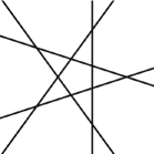
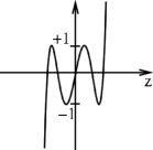
$R_{5}(x,y)$	$T_{5}(z)$	$R_{5}(x,y)+\frac{1}{2}(T_{5}(z)+1)$

Figure 1. A variant of Givental’s and Chmutov’s construction: A regular $5$-gon $R_{5}(x,y)$, the Chebychev polynomial $T_{5}(z)$ and the surface $R_{5}(x,y)+\frac{1}{2}(T_{5}(z)+1)$ with $10\cdot 2+5\cdot 2=30$ nodes.

3. Adaption to Higher Singularities

To adapt Chmutov’s construction (2) to higher singularities of type $A_{j}$, we replace the polynomials $T_{d}(z)$ by polynomials with degenerate critical points.

For the construction of a quintic surface with many cusps, we thus take again the regular $5$-gon $R_{5}(x,y)\in{\mathds{R}}[x,y]$ together with a polynomial $T^{2}_{5}(z)\in{\mathds{R}}[z]$ of degree $5$ with the maximum number of critical points of multiplicity two.

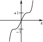
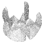
$R_{5}(x,y)$	$T^{2}_{5}(z)$	$R_{5}(x,y)+\frac{1}{2}(T^{2}_{5}(z)+1)$

Figure 2. The construction of a quintic with $15$ cusps.

As the derivative of such a polynomial has degree $4$, the maximum number of such critical points is ${4\over 2}=2$, see fig. 2. The critical values of these two critical points have to be different because a horizontal line through both critical points would intersect the curve in six points counted with multiplicities. Similar to the situation for nodes in (2) the surface $R_{5}(x,y)+\frac{1}{2}(T^{2}_{5}(z)+1)$ has $10{\textup{$\cdot$}}1+5{\textup{$\cdot$}}1=15$ singularities of type $A_{2}$.

As mentioned in the introduction, Barth already constructed another quintic with $15$ cusps [5]. The author constructed a sextic with $35$ cusps in [20], and the appendix gives a sextic with $36$ cusps. But our variant of Chmutov’s construction which will be presented in the following sections gives new lower bounds for the maximum number of $A_{2}$-singularities for all degrees $d\geq 7$. We take surfaces in separated variables defined by polynomials of the form:

(4) $$\textup{Chm}(G^{j}_{d}):=F^{A_{2}}_{d}+G^{j}_{d},$$

where $F^{A_{2}}_{d}(x,y)\in{\mathds{R}}[x,y]$ is the folding polynomial defined in (3) and where $G^{j}_{d}(z)\in{\mathds{C}}[z]$ is a polynomial of degree $d$ with many critical points of multiplicity $j$ with critical values $-1$ and $+1$. E.g., for $j=1$, the ordinary Chebychev polynomials $G^{1}_{d}(z):=T_{d}(z)$ yield to Chmutov’s surfaces with many nodes. In the following sections, we discuss two generalizations of the ordinary Chebychev polynomials to polynomials with critical points of higher multiplicity which give surfaces of degree $d$ with many $A_{j}$-singularities, $j<d$.

4. $j$-Belyi Polynomials via Dessins d’Enfants

The existence of polynomials in one variable with only two different critical values with prescribed multiplicities of the critical points can be established using ideas of Hurwitz [15] based on Riemann’s Existence Theorem. The interest in this subject was renewed by Grothendieck’s Esquisse d’un programme. Nowadays, it is commonly known under the name of Dessins d’Enfants. We will use the following proposition / definition which is basically taken from [1]:

Proposition/Definition 1.

1. A tree (i.e. a graph without cycles) with a prescribed cyclic order of the edges adjacent to each vertex is called a plane tree. A plane tree has a natural bicoloring of the vertices (black/white). If we fix the color of one vertex, then this bicoloring is unique.

2. A polynomial with not more than two different critical values is called a Belyi polynomial.

3. For a given Belyi polynomial $p:{\mathds{C}}\to{\mathds{C}}$ with critical values $c_{1}$ and $c_{2}$, we define the plane tree $PT(p)$ associated to $p$ to be the inverse image $p^{-1}([c_{1},c_{2}])$ of the interval $[c_{1},c_{2}]$, where $p^{-1}(c_{1})$ are the black vertices, and $p^{-1}(c_{2})$ are the white vertices of the tree (see fig. 3).

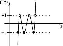
   Figure 3. The ordinary Chebychev polynomial $T_{5}$ with two critical points with critical value $-1$ and two with critical value $+1$. The right picture shows its plane tree $PT(T_{5})$. A vertex with two adjacent edges corresponds to a critical point with multiplicity $1$, a vertex with one adjacent edge corresponds to a non-critical point.

4. For any plane tree, there exists a Belyi polynomial whose critical points have the multiplicities given by the number of edges adjacent to the vertices minus one and vice verca.

We will need the following two trivial bounds concerning critical points:

Lemma 2.

Let $d,j\in{\mathds{N}}$. Let $g\in{\mathds{C}}[z]$ be a polynomial of degree $d$ in one variable with only isolated critical points. Then:

1. The total number of different critical points of $g$ of multiplicity $j$ does not exceed $\lfloor{d-1\over j}\rfloor$.

2. The number of different critical points of $g$ of multiplicity $j$ with the same critical value does not exceed $\lfloor{d\over j+1}\rfloor$. $\Box$

We give a special name to polynomials reaching the first of these bounds:

Definition 3.

Let $d,j\in{\mathds{N}}$ and let $p$ be a Belyi polynomial of degree $d$. We call $p$ a $j$-Belyi polynomial if $p$ has the maximum possible number $\lfloor{d-1\over j}\rfloor$ of critical points of multiplicity $j$.

Example 1.

The ordinary Chebychev polynomials $T^{1}_{d}(z):=T_{d}(z)$ are $1$-Belyi polynomials. $T^{2}_{5}(z)$ in fig. 2 is a $2$-Belyi Polynomial. $\Box$

A special type of $j$-Belyi polynomials are those of degree $j+1$. We will join several plane trees corresponding to such $j$-Belyi polynomials of degree $j+1$ to form larger plane trees in the following sections:

Definition 4.

We call the plane tree corresponding to a $j$-Belyi polynomial of degree $j+1$ a $j$-star. If the center of this tree is a black (resp. white) vertex we call it a $\bullet$- (resp. $\circ$-) centered $j$-star (see fig. 4).

$T^{j}_{j+1}(z)=z^{j+1}-1$  for $j=6$.

Figure 4. The polynomial $T^{j}_{j+1}(z)$ with exactly one critical point $z_{0}=0$ of multiplicity $j$ and critical value $-1$ together with the corresponding $\bullet$-centered $j$-star.

5. The Polynomials $T^{j}_{d}(z)$

A natural generalization of the ordinary Chebychev polynomials to polynomials $G^{j}_{d}(z)$ with degenerate critical points that can be used in the construction of equation (4) on page 4 comes from the following intuitive idea: Take polynomials which look similar to the ordinary Chebychev polynomials (fig. 3), but which have higher vanishing derivatives such that they are $j$-Belyi polynomials.

Example 2.

A $3$-Belyi polynomial of degree $13$ has $\bigl{\lfloor}\frac{13-1}{3}\bigr{\rfloor}=4$ critical points of multiplicity $3$. The polynomial $T^{3}_{13}$ has two critical points with critical value $-1$ and two with critical value $+1$. The plane tree showing the existence of such a polynomial consists of four connected $3$-stars. To show the similarity to the ordinary Chebychev polynomials we draw them in fig. 4 as four bouquets of $1$-stars attached to the plane tree in fig. 3. A straightforward Singular [13] script to compute the equation of $T^{3}_{13}(z)$ can be found on the website [18]. $\Box$

Figure 5. The bicolored plane tree $PT(T^{j}_{d})$ for the polynomial $T^{j}_{d}(z)$ for $j=3$, $d=13$, $k:={d-1\over j}=4$. It consists of $k$ connected $j$-stars. Here, we line them up to show the similarity to the ordinary Chebychev polynomials in fig. 3. See [18] for a Singular [13] script to compute the equation of $T^{3}_{13}(z)$.

Theorem/Definition 5.

Let $d,j\in{\mathds{N}}$ with $d>j$. There exists a polynomial $\mathbf{T^{j}_{d}(z)}$ of degree $d$ with $\lceil{1\over 2}\lfloor{d-1\over j}\rfloor\rceil$ critical points of multiplicity $j$ with critical value $-1$ and $\lfloor{1\over 2}\lfloor{d-1\over j}\rfloor\rfloor$ such critical points with critical value $+1$.

Proof.

The corresponding plane tree $PT(T^{j}_{d})$ can be defined as follows (compare fig. 4). For $d=k\cdot(j+1),\ k\in{\mathds{N}}$, we take $k$ connected $j$-stars. Fixing the center of the first $j$-star to be white, the plane tree has a unique bicoloring. If $d=l+k\cdot(j+1)$ for some $1\leq l\leq j$, we attach another $l$-star to get a polynomial of degree $d$. ∎

Although there is an explicit recursive construction of ordinary Chebychev polynomials and their generalizations to higher dimensions (so-called folding polynomials, see [28]), we do not know a similar explicit construction of the polynomials $T^{j}_{d}(z)$ for $j\geq 2$. To our knowledge, they can only be computed for low degree $d$ until now, e.g. using Groebner Basis. When plugged into the construction (4) on page 4 the existence of the polynomials $T^{j}_{d}$ immediately implies:

Corollary 6.

Let $d,j\in{\mathds{N}}$ with $d>j$. There exist surfaces Chm(T^j_d) := F^A_2_d + 12(T^j_d+1) of degree $d$ with the following number of singularities of type $A_{j}$:   12d(d-1) $\cdot$⌈12⌊d-1j⌋⌉+ 13d(d-3) $\cdot$⌊12⌊d-1j⌋⌋,if  d ≡0 mod3,12d(d-1) $\cdot$⌈12⌊d-1j⌋⌉+ 13(d(d-3)+2) $\cdot$⌊12⌊d-1j⌋⌋otherwise.      □

6. The Polynomials $M^{j}_{d}(z)$

The $j$-Belyi polynomials $T^{j}_{d}(z)$ described in the previous section reach the first bound of lemma 2. The $j$-Belyi polynomials $M^{j}_{d}(z)$ whose existence will be shown in this section also achieve the second bound of this lemma. We start with two examples:

Example 3.

The $2$-Belyi polynomial $T^{2}_{9}(z)$ is the example of the smallest degree from the previous section that does not reach the second bound of lemma 2. The plane tree $PT(M^{2}_{9}(z))$ in fig. 6 shows the existence of a $2$-Belyi polynomial of degree $9$ that achieves this bound.

As in the case of the polynomials $T^{j}_{d}(z)$, it is possible to compute the polynomials $M^{j}_{d}(z)$ explicitly for low $j$ and $d$. For our case $j=2,d=9$ we denote by $u$ the unique critical point with critical value $+1$ and by $b_{0},b_{1},b_{2}$ the three critical points with critical value $-1$. When requiring $b_{2}=0$ (i.e., $M^{2}_{9}(0)=-1$), $M^{2}_{9}(z)$ has the derivative ∂M29∂z(z) = (z-b_0)^2⋅(z-b_1)^2⋅z^2⋅(z-u)^2. Using Singular [13], we find: $u^{9}=18$ and $b_{0}$ and $b_{1}$ are the two distinct roots of $z^{2}-3uz+3u^{2}=0$. Notice that $b_{0},b_{1}\notin{\mathds{R}}$ even if we take $u\in{\mathds{R}}$. $\Box$

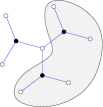
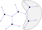
(a)  $PT(M^{2}_{3})$		(b)  $PT(M^{2}_{9})$		(c)  $PT(M^{2}_{15})$

Figure 6. To obtain $PT(M^{2}_{9})$ from the $2$-star $PT(M^{2}_{3})=PT(T^{2}_{3})$, we attach two $\bullet$-centered $2$-stars to one of the $\circ$-vertices (marked by the grey background). The corresponding polynomial $M^{2}_{9}(z)$ has thus $3$ critical points of multiplicity $2$ with critical value $-1$ (the $3$ $\bullet$-centered $2$-stars) and $1$ such point with critical value $+1$ (the only $\circ$-centered $2$-star). $M^{2}_{15}$ has five and two, respectively.

Example 4.

If $d\neq k\cdot(j+1)$ for some $k\in{\mathds{N}}$, the construction of a plane tree corresponding to a polynomial reaching both bounds of lemma 2 is a little more delicate than in the previous example. The cases $PT(M^{2}_{11})$ and $PT(M^{2}_{12})$ in fig. 7 illustrate this. $\Box$

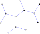
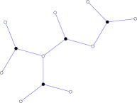
(a)  $PT(M^{2}_{11})$		(b)  $PT(M^{2}_{12})$

Figure 7. $M^{2}_{11}$ and $M^{2}_{12}$ have the same number of critical points of multiplicity $j$. $M^{2}_{12}$ has five ones with critical value $-1$ and only one critical point with critical value $+1$. $M^{2}_{11}$ has three critical points with critical value $-1$ and two with critical value $+1$.

Theorem/Definition 7.

Let $d,j\in{\mathds{N}}$ with $d>j$. There exists a polynomial $\mathbf{M^{j}_{d}(z)}$ of degree $d$ with $\left\lfloor{d\over j+1}\right\rfloor$ critical points of multiplicity $j$ with critical value $-1$ and $\left(\left\lfloor{d-1\over j}\right\rfloor-\left\lfloor{d\over j+1}\right\rfloor\right)$ such critical points with critical value $+1$.

Proof.

The existence of a corresponding plane tree $PT(M^{j}_{d})$ can be shown as follows (compare fig. 6). For $d=j+1$ we define $PT(M^{j}_{d})$ as a $\bullet$-centered $j$-star. For $d=(j+1)+k\cdot j{\textup{$\cdot$}}(j+1),\ k\in{\mathds{N}}$, we attach successively sets of $j$ $\bullet$-centered $j$-stars as illustrated in figure 6. If $d\neq(j+1)+k\cdot j{\textup{$\cdot$}}(j+1)$ for some $k\in{\mathds{N}}$ the existence of plane trees $PT(M^{j}_{d})$ can be shown similarly (see fig. 7). ∎

The existence of the polynomials $M^{j}_{d}(z)$ has two immediate consequences:

Corollary 8.

The bounds in lemma 2 are sharp. $\Box$

It is clear that the polynomials $M^{j}_{d}$ cannot have only real coefficients and only real critical points for $d$ large enough. So, the same holds for the singularities of the surfaces of the following corollary:

Corollary 9.

Let $d,j\in{\mathds{N}}$ with $d>j$. There exist surfaces Chm(M^j_d) := F^A_2_d + M^j_d of degree $d$ with the following number of singularities of type $A_{j}$: 12d(d-1) $\cdot$⌊dj+1⌋+ 13d(d-3) $\cdot$(⌊d-1j⌋-⌊dj+1⌋),if  d ≡0 mod3,12d(d-1) $\cdot$⌊dj+1⌋+ 13(d(d-3)+2) $\cdot$(⌊d-1j⌋-⌊dj+1⌋)otherwise.      □

7. Upper Bounds

To get an idea of the quality of our best lower bounds given by our examples $\textup{Chm}(M^{j}_{d})$ from corollary 9 we compare them with the best known upper bounds: Miyaoka’s bound [22] and Varchenko’s Spectral Bound [27].

7.1. Varchenko’s Spectral Bound

It is well-known that Varchenko’s Spectral Bound $\textup{Var}_{A_{j}}(d)$ for the maximum number of $A_{j}$-singularities [27] is not as good as Miyaoka’s bound for fixed $j$ and large $d$. Although it is known that both bounds can be described by a polynomial of degree three in $d$, we could not find explicit statements for Varchenko’s bound for $j>1$ in the literature. So, we compute these polynomials here using a short Singular [13] script. The code can be downloaded from [18]. In the following, we explain briefly how the algorithm works.

For even degree $d\geq 4$ the spectrum $sp(d)$ of the singularity $x^{d}+y^{d}+z^{d}=0$ in ${\mathds{C}}^{3}$ consists of the spectral numbers $s_{d}(i)={i+2\over d},i=1,2,\dots,3(d-1)-2$, with multiplicities $m_{d}(i)$, where

• $m_{d}(1)=1$,

• $m_{d}(i+1)=m_{d}(i)+1+i,\quad i<d-1$,

• $m_{d}(i+1)=m_{d}(i)+2(i_{mid}-i)+1,\quad d-1\leq i<i_{mid}:={3d\over 2}-2$,

• $m_{d}(3(d-1)-1-i)=m_{d}(i),\quad 1\leq i\leq i_{mid}$ (symmetry of the spectrum).

The spectrum of an $A_{j}$ singularity is also well-known (see e.g. [2, p. 389]). Its spectral numbers are ${j+2\over j+1}$, ${j+3\over j+1}$, …, ${2j+1\over j+1}$, all with multiplicity $1$.

Example 5.

The spectrum $sp(6)$ of the singularity $x^{6}+y^{6}+z^{6}$ is:

$\begin{array}[]{rc@{\ }c@{\ }c@{\ }c@{\ }c@{\ }c@{\ }c@{\ }c@{\ }c@{\ }c@{\ }c@{\ }c@{\ }c@{\ }c@{\ }c@{\ }c@{\ }c@{\ }c@{\ }c@{\ }c@{\ }c@{\ }c@{\ }c@{\ }c@{\ }c@{\ }c@{\ }c@{\ }c@{\ }c@{\ }c@{\ }c@{\ }c@{\ }c@{\ }c@{\ }c}\footnotesize i&1&&2&&3&&4&&5&&6\hfil\ &&7&&8&&9&&10&&11&&12\hfil\ &&13\\[1.99997pt] \footnotesize\textup{spectral number}\ s_{i}&3\over 6&&4\over 6&&5\over 6&&6\over 6&&7\over 6&&8\over 6\hfil\ &&9\over 6&&10\over 6&&11\over 6&&12\over 6&&13\over 6&&14\over 6\hfil\ &&15\over 6\\[5.69046pt] \footnotesize\textup{multiplicity}\ m_{i}&1&&3&&6&&10&&15&&18\hfil\ &&19&&18&&15&&10&&6&&3\hfil\ &&1\\[2.84544pt] \end{array}$

The spectral numbers of the $A_{2}$-singularity are: $\frac{8}{6},\frac{10}{6}$, both with multiplicity $1$. $\Box$

To compute Varchenko’s bound we have to choose an open interval $I=(\frac{i_{l}+2}{d},\frac{i_{r}+2}{d})$ of length $1$ of the spectrum $sp(d)$ that contains all spectral numbers of the $A_{j}$ singularity and such that the sum of the multiplicities of the spectral numbers in the interval is minimal. Then we have to sum up all the multiplicities in this interval and divide by $j$.

Let us write $d=k{\textup{$\cdot$}}(j+1)+l$. Then we may choose $I:=(\frac{i_{r}+2-d}{d},\frac{i_{r}+2}{d})$, where $i_{r}:=k{\textup{$\cdot$}}(2j+1)+\left\lfloor{l\cdot(2j+1)\over j+1}\right\rfloor-1$. We introduce some notations: $n_{l}:=i_{mid}-(d-1)$, $n_{r}:=i_{r}-i_{mid}-1$, $n_{ll}:=d-1-n_{l}-n_{r}$, $m_{mid}=\sum_{i=1}^{d-1}i+(\frac{d}{2}-1)^{2}$. Using these we can compute Varchenko’s bound $\textup{Var}_{A_{j}}(d)$ for the maximum number of $A_{j}$-singularities on a surface of degree $d$ in ${\mathds{P}}^{3}$ for the case $d,j\in{\mathds{N}}$ with $d\geq 4$:

(5) $$\quad\begin{array}[]{r@{\ }c@{\ }l}\textup{Var}_{A_{j}}(d)&=&\Bigl{\lfloor}\frac{1}{j}{\textup{$\cdot$}}\Bigl{(}\frac{1}{2}{\textup{$\cdot$}}\bigl{(}\sum_{i=1}^{d-1}i\ +\sum_{i=1}^{d-1}i^{2}\ -\sum_{i=1}^{d-1-n_{ll}}i\ -\sum_{i=1}^{d-1-n_{ll}}i^{2}\bigr{)}\\ &&+(n_{r}+n_{ll})\cdot m_{mid}\ -\sum_{i=1}^{n_{r}}i^{2}\ -\sum_{i=1}^{n_{l}-1}i^{2}\Bigr{)}\Bigr{\rfloor}.\quad\qquad\qquad\Box\end{array}$$

Example 6.

Let us look at the case $d=6,j=2$ as in example 5. In this case, the constants used above have the following values: $k=2$, $l=0$, $i_{r}=9$, $i_{l}=3$, $i_{mid}=7$, $n_{l}=2$, $n_{r}=1$, $n_{ll}=2$, $m_{mid}=19$. We can now easily compute the bound $\textup{Var}_{A_{2}}(d)$ in (5) for $d=6$ (compare the table in example 5):     Var_A_2(6)  =  ⌊  12 ⋅( ⏟15+55-6-142_=10+15 +⏟3 ⋅19 -1 -1_=18+19+18 )⌋ =  40.    □

Using some summation formulas we find the following bounds for $d\geq 4$. Some of these are well-known, but we list them because we could not find them in the literature:

$\mu_{A_{2}}(d)\leq\textup{Var}_{A_{2}}(d)=\left\{\begin{array}[]{ll}\frac{31}{108}d^{3}-\frac{25}{36}d^{2}+\frac{1}{2}d,&d\equiv 0\mod 3,\\[1.99997pt] \frac{31}{108}d^{3}-\frac{31}{36}d^{2}+\frac{17}{18}d-\frac{10}{27},&d\equiv 1\mod 3,\\[1.99997pt] \frac{31}{108}d^{3}-\frac{7}{9}d^{2}+\frac{3}{4}d-\frac{5}{27},&d\equiv 2\mod 3.\end{array}\right.$ • $\mu_{A_{3}}(d)\leq\textup{Var}_{A_{3}}(d)=\left\{\begin{array}[]{ll}\frac{235}{1152}d^{3}-\frac{49}{96}d^{2}+\frac{13}{36}d,&d\equiv 0\mod 4,\\[1.99997pt] \frac{235}{1152}d^{3}-\frac{235}{384}d^{2}+\frac{785}{1152}d-\frac{35}{128},&d\equiv 1\mod 4,\\[1.99997pt] \frac{235}{1152}d^{3}-\frac{37}{64}d^{2}+\frac{173}{288}d-\frac{3}{16},&d\equiv 2\mod 4,\\[1.99997pt] \frac{235}{1152}d^{3}-\frac{209}{384}d^{2}+\frac{569}{1152}d-\frac{35}{384},&d\equiv 3\mod 4.\end{array}\right.$ The formulas are not correct for $d=3$ for some $j$ because the spectrum of the $x^{3}+y^{3}+z^{3}=0$ singularity does not have enough spectral numbers to fit into the description above.

7.2. Miyaoka’s Bound

In [22] Miyaoka gives the following upper bound for the maximum number $\mu_{A_{j}}(d)$ of $A_{j}$-singularities on a surface of degree $d$ in ${\mathds{P}}^{3}$:

(6) $$\mu_{A_{j}}(d)\leq\textup{Miy}_{A_{j}}(d):={2\over 3}{j+1\over j(j+2)}d(d-1)^{2}\approx{2\over 3}{j+1\over j(j+2)}d^{3}.$$

Our variants $\textup{Chm}(M^{j}_{d})$ of Chmutov’s surfaces give a lower bound of approximately μ_A_j(Chm(M^j_d)) ≈3j+26j(j+1)d^3 such singularities for large $d$. This is at least $75\%$ of the best known upper bound:

Corollary 10.

Let $j\in{\mathds{N}}$. For large degree $d$, the quotient of the number of $A_{j}$-singularities on our surfaces $\textup{Chm}(M^{j}_{d})$ and the best known upper bound $\textup{Miy}_{A_{j}}(d)$ is: μAj(Chm(Mjd))MiyAj(d) ≈(j+2)(3j+2)4(j+1)2. This quotient is greater than $\frac{3}{4}$ for all $j\geq 1$, the limit for $j\to\infty$ is also $\frac{3}{4}$. $\Box$

8. Generalization to Higher Dimensions

It is possible to generalize the construction of surfaces with many $A_{j}$-singularities described in the previous sections to ${\mathds{P}}^{n}$, $n\geq 4$. It turns out that for $n\geq 5$, the folding polynomials $F^{A_{2}}_{d}(x,y)$ are no longer the best choice: Even for nodal hypersurfaces, the folding polynomials $F^{B_{2}}_{d}(x,y)$ lead to better lower bounds.

8.1. Nodal Hypersurfaces in ${\mathds{P}}^{n}$, $n\geq 4$

As Chmutov mentioned in [9], his idea to use the folding polynomials gives the best lower bounds for the maximum number of nodes on hypersurfaces in ${\mathds{P}}^{4}$ of degree $d$ for $d$ large enough. As Chmutov certainly knew, this can be generalized further to higher dimensions similar to Givental’s construction of cubics in ${\mathds{P}}^{n}$ [2, p. 419]:

(7) $$\textup{Chm}^{n}(F_{d}^{A_{2}}):\quad\sum_{i=0}^{\lfloor{n-2\over 2}\rfloor}(-1)^{i}F^{A_{2}}_{d}(x_{2i},x_{2i+1})=(n\ \textup{mod}\ 2){\textup{$\cdot$}}\frac{1}{2}(T_{d}(x_{n-1})+1).$$

In some cases, e.g. $n=5$, it is better to replace the sign $(-1)^{i}$ in that formula by $1$ and to adjust the coefficients on the right-hand side. But for $n\geq 5$, the asymptotic behaviour (see table 4) of Chmutov’s older series TChm^n_d: ∑_i=0^n-1 T_d(x_i) = -(n  mod  2). (see [2, p. 419]) still gives more nodes (exactly $\bigl{(}\frac{d-1}{2}\bigr{)}^{n}{\textup{$\cdot$}}{n\choose n/2}$ for odd degree). The reason for this is that the plane curve $T_{d}(x)+T_{d}(y)$ has the critical values $-1,0,+1$ of which the two non-zero ones sum up to zero. Nevertheless, for small degree $d$ the hypersurfaces $\textup{Chm}^{n}(F_{d}^{A_{2}})$ are better.

In order to improve the asymptotic behaviour of the lower bound slightly, we can use a folding polynomial associated to another root system. Such polynomials were described in [28], and their critical points were studied in [7] analogous to the case of $A_{2}$ treated by Chmutov in [9]. It turns out that the folding polynomials $F_{d}^{B_{2}}(x,y)$ associated to the root system $B_{2}$ are best suited for our purposes. They can be defined recursively as follows: $F_{0}^{B_{2}}:=1$,  $F_{1}^{B_{2}}:=\frac{1}{4}y$, $F_{2}^{B_{2}}:=\frac{1}{4}y^{2}-\frac{1}{2}(x^{2}-2y-4)-1$,  $F_{3}^{B_{2}}:=\frac{1}{4}y^{3}-\frac{3}{4}y(x^{2}-2y-4)-\frac{3}{4}y,$

(8) $$F_{d}^{B_{2}}:=y(F_{d-1}^{B_{2}}+F_{d-3}^{B_{2}})-(2+(x^{2}-2y-4))F_{d-2}^{B_{2}}-F_{d-4}^{B_{2}}.$$

These polynomials have exactly three different critical values: $-1$, $0$, $+1$. The numbers of critical points of $F_{d}^{B_{2}}$ are: $d\choose 2$ with critical value $0$, $\lfloor\frac{(d-1)}{2}\rfloor\lfloor\frac{d}{2}\rfloor$ with critical value $-1$. The use of these polynomials improves the asymptotic behaviour (for $d$ large) of the best known lower bound for the maximum number of nodes only slightly. In fact, the coefficient of the highest order term does not change (see table 4). Nevertheless, we want to mention:

Proposition 11.

Let $n\geq 2$, $d\geq 3$. Then: $\mu(\textup{Chm}^{n}(F_{d}^{B_{2}}))>\mu(\textup{TChm}^{n}_{d}).$

Table 2. The asymptotic behaviour of the number of nodes on variants of Chmutov’s hypersurfaces in ${\mathds{P}}^{n}$. As Chmutov already realized in [9], the $\textup{Chm}^{n}(F_{d}^{A_{2}})$ are only better for $n=3,4$. For $n\geq 5$, the best lower bounds are given by our variant $\textup{Chm}^{n}(F_{d}^{B_{2}})$ which improves Chmutov’s oldest examples $\textup{TChm}^{n}_{d}$ slightly.

It is not true that the folding polynomials $F_{d}^{A_{2}}$ and $F_{d}^{B_{2}}$ are the best possible choices in all cases. Indeed, for $d=5$, a regular fivegon leads to more nodes. For $d=3,4$ there are better constructions for nodal hypersurfaces in ${\mathds{P}}^{n}$ known [12]. In fact, Kalker [16] already noticed that Varchenko’s upper bound is exact for $d=3$.

8.2. Hypersurfaces in ${\mathds{P}}^{n}$ with $A_{j}$-Singularities, $j\geq 2,n\geq 4$

Similar to the case of surfaces, we can adapt the equations for the nodal hypersurfaces to get hypersurfaces $\textup{Chm}^{j,n}(F_{d}^{B_{2}})$ (or $\textup{Chm}^{j,n}(F_{d}^{A_{2}})$, $\textup{TChm}^{j,n}_{d}$) with many $A_{j}$-singularities:

(9) $$\textup{Chm}^{j,n}(F_{d}^{B_{2}}):\sum_{i=0}^{\lfloor{n-3\over 2}\rfloor}F^{B_{2}}_{d}(x_{2i},x_{2i+1})=\left\{\begin{array}[]{@{}l@{\ }l}T_{d}(x_{n-2})+M^{j}_{d}(x_{n-1}),&n\,\textup{even}\\ -\frac{1}{2}(M^{j}_{d}(x_{n-1})+1),&n\,\textup{odd}.\end{array}\right.$$

This leads to the asymptotic behaviour given in table 4. Notice that we usually get fewer singularities if we add a sign $(-1)^{i}$ in the sum in contrast to equation (7) where the alternating sign is often better because the folding polynomial $F_{d}^{A_{2}}$ has other critical values than $F_{d}^{B_{2}}$.

Table 3. The asymptotic behaviour of the number of $A_{j}$-singularities on a hypersurface of degree $d$ in ${\mathds{P}}^{n}$. $\textup{Chm}^{j,n}(F_{d}^{B_{2}})$ is better than $\textup{Chm}^{j,n}(F_{d}^{A_{2}})$ for $n\geq 6$.

Of course, for small $d,n,j$, it is often easy to write down better lower bounds. E.g., if $n$ is even and $d$ is small, it is often better to replace $T_{d}(x_{n-2})+M^{j}_{d}(x_{n-1})$ by a plane curve with the maximum known number of cusps. For some specific values of $d$, $j\geq 2$, $n\geq 4$ there are even better lower bounds known. E.g., Lefschetz [21] constructed a cubic hypersurface in ${\mathds{P}}^{4}$ with $5$ cusps which is the maximum possible number.

Appendix A On Variants of Segre’s Construction

In 1952, B. Segre [26] introduced a construction of surfaces with many singularities using pull-back under a branched covering $\Omega_{2}^{3}$. Many interesting nodal surfaces can be constructed in this way, e.g., sextics with $1$ up to $64$ nodes [8] and even Barth’s sextic with $65$ nodes [3].

Shortly after B. Segre’s well-known discovery, Gallarati [11] generalized this construction to higher dimensions and higher singularities:

(10) $$\Omega_{j+1}^{n}:\ {\mathds{P}}^{n}\to{\mathds{P}}^{n},\ (x_{0}:x_{1}:\cdots:x_{n})\mapsto(x_{0}^{j+1}:x_{1}^{j+1}:\cdots:x_{n}^{j+1}),\quad j\in{\mathds{N}}.$$

Gallarati does not give a general formula for the number and type of singularities one obtains using this map. He only computes some examples. But it is easy to derive a formula for hypersurfaces with $A_{j}$-singularities similar to B. Segre’s case of nodal surfaces in ${\mathds{P}}^{3}$: Let $F_{0}$ be a hypersurface in ${\mathds{P}}^{n}$ of degree $d_{0}$ with $k_{0}$ singularities of type $A_{j}$. Take $n+1$ general hyperplanes tangent to $F_{0}$ as the coordinate $(n+1)$-hedron. The degree of the map $\Omega_{j+1}^{n}$ is $(j+1)^{n}$ away from the coordinate hyperplanes. It is $(j+1)^{n-1}$ on a general intersection point of two of the coordinate hyperplanes, and $(j+1)^{n-i},i=2,3,\dots,n,$ for even more special points on the coordinate hyperplanes. For our generic choice of coordinate hyperplanes tangent to $F_{0}$ the pull-back under $\Omega_{j+1}^{n}$ thus gives a hypersurface $F_{1}$ in ${\mathds{P}}^{n}$ of degree $d_{1}:=(j+1){\textup{$\cdot$}}d_{0}$ with

(11) $$\mu_{A_{j}}(F_{1})=(j+1)^{n}{\textup{$\cdot$}}k_{0}+(n+1){\textup{$\cdot$}}(j+1)^{n-1}$$

singularities of type $A_{j}$. Applying the same construction to $F_{1}$, we obtain a hypersurface $F_{2}$ in ${\mathds{P}}^{n}$ of degree $d_{2}:=(j+1)^{2}{\textup{$\cdot$}}d_{0}$ with μ_A_j(F_2) = (j+1)^n((j+1)^n$\cdot$k_0 + (n+1)$\cdot$(j+1)^n-1) + (n+1)(j+1)^n-1 singularities of type $A_{j}$. Iterating this, we get a hypersurface $F_{i}$ of degree $d_{i}:=(j+1)^{i}{\textup{$\cdot$}}d_{0}$ with μ_A_j(F_i) = (j+1)^ni$\cdot$k_0 + n+1j+1⋅((j+1)n(i+1)-1(j+1)n-1 - 1) singularities of type $A_{j}$. Asymptotically, we thus have:

(12) $$\mu_{A_{j}}(F_{i})\approx\frac{1}{d_{0}^{n}}{\textup{$\cdot$}}\left(k_{0}+\frac{(n+1){\textup{$\cdot$}}(j+1)^{n-1}}{(j+1)^{n}-1}\right){\textup{$\cdot$}}d_{i}^{n}\quad\textup{for}\ i\ \textup{large}.$$

For $n\geq 3$, this lower bound is asymptotically not as good as ours presented in the main text. But for low degree, B. Segre’s method sometimes gives more singularities: E.g., when applying $\Omega_{j+1}^{3}$ to a smooth quadric, (11) yields to:

Corollary 12.

Let $j\in{\mathds{N}}$. There exist surfaces of degree $d=2{\textup{$\cdot$}}(j+1)$ with $4{\textup{$\cdot$}}(j+1)^{2}$ singularities of type $A_{j}$.

E.g., for $n=3,j=2$, we obtain $\mu_{A_{2}}(6)\geq 36$, and with Miyaoka’s upper bound: $36\leq\mu_{A_{2}}(6)\leq 37$. For $n=2$, our construction presented in subsection 8.2 only leads to plane curves of degree $d$ with $\approx\frac{1}{4}{\textup{$\cdot$}}d^{2}$ cusps whereas the generalization of B. Segre’s construction gives $\approx\frac{9}{32}{\textup{$\cdot$}}d^{2}$ such singularities when starting with a smooth conic. This idea was taken up later by several people. To our knowledge, the currently best result is due to Vik. S. Kulikov [17]. He used a quartic with three cusps as a starting point. At every other iteration step he was able to choose a bitangent to the curve as one of the coordinate axes. This yields to approximately $\frac{283}{60\cdot 16}{\textup{$\cdot$}}d^{2}$ cusps. So, in the case of plane curves of degree $d$, variants of B. Segre’s idea still give the best known general lower bound for the maximum number $\mu_{A_{2}}^{2}(d)$ of cusps.

In higher dimensions, our construction gives a better lower bound than this generalization of B. Segre’s construction. Notice that it might be able to adapt B. Segre’s construction similar to the case of curves: In the case of surfaces, it might be possible to choose triple tangent planes as coordinate planes. But even when starting from a $36$-cuspidal sextic this would yield to surfaces with less cusps.

Finally, we want to mention that it is easy to compute how many singularities we need to improve the best known lower bounds using the formula (12). Let us look at nodal surfaces: To improve Chmutov’s lower bound $\approx\frac{5}{12}d^{3}$ for the maximum number of nodes on a surface of degree $d$, it suffices to construct a surface of degree $d_{0}$ with $k_{0}$ nodes, s.t. $k_{0}>\frac{5}{12}d_{0}^{3}-\frac{16}{7}$. Comparing this with Miyaoka’s upper bound, we find, e.g., that a $13652$-nodal surface of degree $32$ or a $109225$-nodal surface of degree $64$ would be sufficient.

References

- [1] N. Adrianov and A. Zvonkin. Composition of Plane Trees. Acta Applicandae Mathematicae, 52:239–245, 1998.
- [2] V.I. Arnold, S.M. Gusein-Zade, and A.N. Varchenko. Singularities of Differentiable Maps, volume II. Birkhäuser, 1985.
- [3] W. Barth. Two Projective Surfaces with Many Nodes, Admitting the Symmetry of the Icosahedron. J. Algebraic Geom., 5(1):173–186, 1996.
- [4] W. Barth. K3 Surfaces with Nine Cusps. Geom. Dedicata, 72(2):171–178, 1998.
- [5] W. Barth. A Quintic Surface with Three-Divisible Cusps. Preprint, Erlangen, 2000.
- [6] W. Barth and S. Rams. Cusps and Codes. Preprint, math.AG/0403018, 2004.
- [7] S. Breske. Konstruktion von Flächen mit vielen reellen Singularitäten mit Hilfe von Faltungspolynomen. Diploma Thesis. University of Mainz, 2005. Available from [18].
- [8] F. Catanese and G. Ceresa. Constructing Sextic Surfaces with a given number of Nodes. J. Pure and Appl. Algebra, 23:1–12, 1982.
- [9] S.V. Chmutov. Examples of Projective Surfaces with Many Singularities. J. Algebraic Geom., 1(2):191–196, 1992.
- [10] S.V. Chmutov. Extremal distributions of critical points and critical values. In D. T. Lê, K. Saito, and B. Teissier, editors, Singularity Theory, pages 192–205, 1995.
- [11] D. Gallarati. Alcune riflessioni intorno ad una nota del Prof. B. Segre. Atti Acc. Ligure, 9:106–112, 1952.
- [12] V.V. Goryunov. Symmetric quartics with many nodes. Adv. Soviet Math., 21:147–161, 1994.
- [13] G.-M. Greuel, G. Pfister, and H. Schönemann. Singular 2.0. A Computer Algebra System for Polynomial Computations, Centre for Computer Algebra, Univ. Kaiserslautern, 2001. http://www.singular.uni-kl.de.
- [14] S. Holzer and O. Labs. Illustrating the Classification of Real Cubic Surfaces. Preprint, University of Mainz, Accepted for Publication in the Proceedings of the AGGM 2004, 2005.
- [15] A. Hurwitz. Ueber Riemann’sche Flächen mit gegebenen Verzweigungspunkten. Math. Ann., 39:1–61, 1891.
- [16] T. Kalker. Cubic Fourfolds with fifteen Ordinary Double Points. PhD thesis, Leiden, 1986.
- [17] Vik.S. Kulikov. Generalized Chisini’s Conjecture. Proc. Steklov Math. Inst., 241:110–119, 2003.
- [18] O. Labs. Algebraic Surface Homepage. Information, Images and Tools on Algebraic Surfaces. www.AlgebraicSurface.net, 2003.
- [19] O. Labs. A Septic with Real Nodes. Preprint, math.AG/0409348, 2004.
- [20] O. Labs. A Sextic with Cusps. Preprint, math.AG/0502520, 2005.
- [21] S. Lefschetz. On the with Five Nodes of the Second Species in . Bull. Amer. Math. Soc., 18(2):384–386, 1912.
- [22] Y. Miyaoka. The Maximal Number of Quotient Singularities on Surfaces with Given Numerical Invariants. Math. Ann., 268:159–171, 1984.
- [23] S. Rams. On Quartics with Three-Divisible Sets of Cusps. Manuscr. Math., 111(1):29–41, 2003.
- [24] K. Rohn. Die Flächen vierter Ordnung hinsichtlich ihrer Knotenpunkte und ihrer Gestaltung. Number IX in Preisschriften der Fürstlich Jablonowski’schen Gesellschaft. Leipzig, 1886.
- [25] L. Schläfli. On the Distribution of Surfaces of the Third Order into Species, in Reference to the Presence or Absence of Singular Points and the Reality of their Lines. Philos. Trans. Royal Soc., CLIII:193–241, 1863.
- [26] B. Segre. Sul massimo numero di nodi delle superficie algebriche. Atti. Acc. Ligure, 10:15–22, 1952.
- [27] A.N. Varchenko. On the Semicontinuity of the Spectrum and an Upper Bound for the Number of Singular Points of a Projective Hypersurface. J. Soviet Math., 270:735–739, 1983.
- [28] W.D. Withers. Folding Polynomials and Their Dynamics. Amer. Math. Monthly, 95:399–413, 1988.
- [29] J.-G. Yang. Enumeration of Combinations of Rational Double Points on Quartic Surfaces. AMS/IP Studies in Advanced Mathematics, 5:275–312, 1997.