Knot Polynomials and Knot Homologies

Abstract.

This is an expository paper discussing some parallels between the Khovanov and knot Floer homologies. We describe the formal similarities between the theories, and give some examples which illustrate a somewhat mysterious correspondence between them.

1. Introduction

The past few years have seen considerable growth in the theory of what might be called “knot homologies.” Roughly speaking, these invariants are homological versions of the now–classical knot polynomials — the Alexander polynomial, the Jones polynomial, and their mutual generalization, the HOMFLY polynomial. As a first approximation, we might say that a knot homology is a bigraded homology group $G(K)$ associated to a knot $K\subset S^{3}$. The two gradings are a “homological grading” (the usual sort of grading one expects on a chain complex) and a “filtration grading.” If we take the filtered Euler characteristic of $G(K)$, we recover the corresponding knot polynomial.

As our understanding of these objects evolves, it seems likely that the definition of a knot homology will evolve with it. As a first approximation, however, we offer the following:

Definition.

A knot homology is a theory which assigns to an oriented link $L\subset S^{3}$ together with some auxiliary data $\mathcal{D}$ a filtered chain complex $\mathcal{C}(L,\mathcal{D})$ satisfying the following properties:

1. The filtered Euler characteristic of $\mathcal{C}(L,\mathcal{D})$ is a “classical” polynomial invariant of $L$.

2. The filtration on $\mathcal{C}(L,\mathcal{D})$ gives rise to a spectral sequence $\{E_{i},d_{i}\}\ (i>0)$. For all $i\geq 2$, $E_{i}$ does not depend on the choice of auxiliary data $\mathcal{D}$, and is thus an invariant of the link $L$.

3. The homology of the total complex $\mathcal{C}(L,\mathcal{D})$ depends only on coarse information about $L$, such as the number of components and their linking numbers.

In this formulation, the group $G(K)$ mentioned above is the $E_{2}$ term of the spectral sequence.

One thing that makes this definition attractive is the fact that the known examples arise from rather different areas of mathematics. The idea that such an object might exist at all is due to Mikhail Khovanov. In [10] he constructed a bigraded homology theory which I’ll call $Kh(K)$, whose filtered Euler characteristic is the unnormalized Jones polynomial of $K$. More recently, Khovanov and Rozansky [12] have constructed an infinite family of of such knot homologies, one for each $n>0$. Their filtered Euler characteristics give certain specializations of the HOMFLY polynomial. (When $n=2$ one recovers $Kh(K)$.) Our other example of a knot homology comes from gauge theory; more precisely, from the Heegaard Floer homology introduced by Peter Ozsváth and Zoltán Szabó [19]. This theory naturally gives rise to a bigraded homology theory known as the knot Floer homology [21], [28], which I’ll denote by $\widehat{HFK}(K)$. Its filtered Euler characteristic is the Alexander polynomial of $K$, which corresponds to the case $n=0$ missing from Khovanov and Rozansky’s construction.

At a first glance, the two types of knot homologies appear to be quite different. Although they share the formal properties listed above, they are defined and computed in very different ways, and things which are easy to see in one theory may be quite unexpected in the other. For example, it was obvious from the start that $\widehat{HFK}$ is the $E_{2}$ term of a spectral sequence, but the corresponding fact for $Kh$ was discovered by Lee in [14], several years after the appearance of [10]. (For the Khovanov-Rozansky theories, this result is due to Gornik [7].) On closer inspection, however, a more subtle correspondence between the two theories begins to appear. This correspondence has guided much of my own research in this area. In particular, it led to the discovery of a relation between the Khovanov homology and the slice genus, which was the subject of my talk at McMaster. Rather than simply rehash this material, which is already covered in [29], I thought I would try to explain where it came from.

The main goal of this paper, then, is to describe the above-mentioned correspondence between the Khovanov homology and the knot Floer homology, and to give some examples to convince the reader that it is an interesting one. This correspondence does not hold for all knots, but it is common enough that the author feels that there must be some sort of explanation. Perhaps someone who reads this paper will be able to provide one. To properly explain the correspondence between the two theories, one must summarize a number of basic facts about them. As a secondary goal, we have tried to make this summary self-contained and accessible to anyone interested in learning about knot homologies.

The rest of the paper is organized as follows. We begin in section 2 with a brief review of some facts about filtered chain complexes. Sections 3 and 4 describe the basic properties of the knot Floer homology and the Khovanov homology, respectively. We do not attempt to give definitions, but instead focus on the formal properties of these theories, their relation with classical models for the Alexander and Jones polynomials, and methods of computation. In section 5, we describe the correspondence we have in mind, and give some reasons for believing that it is interesting. Finally, in sections 6 and  7, we describe some examples of knots for which the correspondence is known to hold, as well as a few cases for which it fails.

The author would like to thank Matthew Hedden, Peter Kronheimer, Ciprian Manolescu, Peter Ozsváth, and Zoltán Szabó for many helpful conversations, and Hans Boden, Ian Hambleton, Andrew Nicas, and Doug Park for putting together a great conference.

2. Preliminaries on Filtered Complexes

We begin by establishing some notation and conventions related to filtered chain complexes. Let $(\mathcal{C},d)$ be a chain complex freely generated over ${\mathbf{Z}}$ by a finite set of generators $\{x_{i}\}$. We say that ${\mathcal{C}}$ is a bigraded complex with homogenous generators $\{x_{i}\}$ if we are given two gradings $u:\{x_{i}\}\to{\mathbf{Z}}$ and $f:\{x_{i}\}\to{\mathbf{Z}}$ with the property that if

$$d(x_{i})=\sum_{j}a_{ij}x_{j}$$

then $u(x_{j})=u(x_{i})-1$ and $f(x_{j})\leq f(x_{i})$ whenever $a_{ij}\neq 0$. We refer to $u$ as the homological grading on $\mathcal{C}$, and $f$ as the filtration grading. The filtration grading defines a filtration $\{\mathcal{F}_{n}\}$ on $\mathcal{C}$, simply by setting $\mathcal{F}_{n}=\text{span}{{\thinspace}}\{x_{i}{{\thinspace}}|{{\thinspace}}f(x_{i})\leq n\}.$ We refer to $\mathcal{F}$ as a downward filtration. (If $f(d(x))$ was always greater than $f(x)$, the result would be an upward filtration.)

Definition 2.1.

The filtered Euler characteristic of $\mathcal{C}$ is defined to be the sum

$$\sum_{i}(-1)^{u(x_{i})}f^{f(x_{i})}.$$

It is an element of the Laurent series ring ${\mathbf{Z}}[f]$.

The filtration $\mathcal{F}$ on $\mathcal{C}$ gives rise to a spectral sequence, which can be explicitly described as follows. We decompose the differential $d$ in terms of the preferred basis $\{x_{i}\}$, setting

$$d(x_{i})=d_{0}(x_{i})+d_{1}(x_{i})+d_{2}(x_{i})+\ldots$$

where

$$d_{n}(x_{i})=\sum a_{ij}x_{j}$$

with $f(x_{j})=f(x_{i})-n$. Since the number of $x_{i}$’s is finite, all but finitely many of the $d_{n}$ are $0$. From the identity $d^{2}=0$, we conclude that $d_{0}^{2}=0$ as well, so $\mathcal{C}_{0}=(\mathcal{C},d_{0})$ is a chain complex. Then the identity $d_{0}d_{2}+d_{1}^{2}+d_{2}d_{0}=0$ implies that $\mathcal{C}_{1}=(H(\mathcal{C}_{0}),d_{1})$ is a chain complex. Repeating, we obtain a sequence of chain complexes $\mathcal{C}_{i+1}=(H(\mathcal{C}_{i}),d_{i})$ which eventually converges to $H(\mathcal{C})$. The complex $(\mathcal{C}_{i},d_{i})$ is generally referred to as the $E_{i+1}$ term of the spectral sequence.

If we are working with coefficients in a field, it is not difficult to show (c.f. section 5.1 of [28]) that $\mathcal{C}_{1}$ can be endowed with a differential $\overline{d}_{1}$ in such a way that $(\mathcal{C}_{1},\overline{d}_{1})$ is chain homotopy equivalent to $(\mathcal{C},d)$. $(\mathcal{C}_{1},\overline{d}_{1})$ is again a bigraded complex, and the resulting spectral sequence is isomorphic to our original spectral sequence $(\mathcal{C}_{i},d_{i})$.

In the definition of the known knot homologies, the following situation arises. Starting from a link $L$ plus a choice of some additional data $\mathcal{D}$, one obtains a bigraded complex $\mathcal{C}$. A different choice of data $\mathcal{D^{\prime}}$ gives rise to a different chain complex $\mathcal{C}^{\prime}$ together with a filtered chain map $\phi:\mathcal{C}\to\mathcal{C}^{\prime}$. It is easy to see that $\phi$ induces maps $\phi_{i}:\mathcal{C}_{i}\to\mathcal{C}^{\prime}_{i}$. One checks directly that the map $\phi_{1}$ is an isomorphism; it then follows from general principles [17] that $\phi_{i}$ is an isomorphism for all $i>0$. The knot homology is the bigraded complex $\mathcal{H}(L)=({\mathcal{C}}_{1},\overline{d}_{1})$; it is well-defined up to filtered isomorphism.

Since $\mathcal{H}(L)$ will be the primary object of our attention, we make a few comments specific to it. To begin with, observe that $\mathcal{C}_{0}$ decomposes as a direct sum of complexes

$$\mathcal{C}_{0}=\bigoplus\mathcal{C}_{0}^{j}$$

where $\mathcal{C}_{0}^{j}$ is generated by those $x_{i}$ with $f(x_{i})=j$. As a group, then, we can decompose $\mathcal{C}_{1}=\bigoplus H(\mathcal{C}_{0}^{j})$. When we want to distinguish the summands in $\mathcal{H}(L)$, we denote $H_{i}(\mathcal{C}_{0}^{j})$ by $\mathcal{H}_{i}(L,j)$ .

It is often convenient to represent $\mathcal{H}(L)$ by its filtered Poincaré polynomial:

Definition 2.2.

The filtered Poincaré polynomial of $\mathcal{H}$ is given by

$$P_{\mathcal{H}(L)}(f,u)=\sum_{i,j}{{\thinspace}}({{\text{rank}\ }}\mathcal{H}_{i}(L,j))\ u^{i}f^{j}.$$

It is a Laurent polynomial in $u$ and $f$.

If we substitute $u=-1$, the filtered Poincaré polynomial reduces to the filtered Euler characteristic. When ${{\text{rank}\ }}\mathcal{H}_{i}(L,j)=1$, we will often use the shorthand $u^{i}f^{j}$ to refer to a generator of this group.

3. The Knot Floer Homology

Let $K$ be a knot in $S^{3}$. The knot Floer homology $\widehat{HFK}(K)$ is a bigraded chain complex equipped with a homological grading $u$ and a filtration grading $t$, which is also known as the Alexander grading. Conventionally, the Alexander grading is chosen so as to define a downward filtration on $\widehat{HFK}(K)$. The filtered Euler characteristic of $\widehat{HFK}(K)$ is the Alexander polynomial $\Delta_{K}(t)$, and the homology of the complex $\widehat{HFK}(K)$ is a single copy of ${\mathbf{Z}}$ in homological grading $0$.

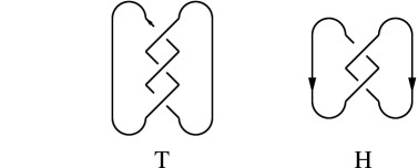
Figure 1. The positive trefoil and Hopf link.

3.1. Examples

Let $U$ be the unknot. The complex $\widehat{HFK}(U)$ is generated by a single element whose Alexander and homological gradings are both equal to zero. The differential on this complex is necessarily trivial.

Let $T$ be the positive trefoil knot shown in Figure 1. Then $\widehat{HFK}(T)$ is generated by three elements $x_{-1},x_{0}$, and $x_{1}$, where $t(x_{i})=i$ and $u(x_{i})=i-1$. The filtered Poincaré polynomial is given by

$$P_{\widehat{HFK}(T)}(t,u)=t+t^{0}u^{-1}+t^{-1}u^{-2}.$$

Substituting $u=-1$, we recover the filtered Euler characteristic, which is the Alexander polynomial of $T$:

$$\Delta_{T}(t)=t-1+t^{-1}.$$

The action of $d$ is given by $d(x_{-1})=d(x_{1})=0$, $d(x_{0})=x_{-1}$.

3.2. Symmetry and the $\delta$-grading

It is well known that the Alexander polynomial is symmetric under the involution which sends $t\mapsto t^{-1}$. $\widehat{HFK}$ is endowed with an analogous symmetry. To descibe the behavior of the homological grading under this symmetry, it is convenient to introduce a third grading on the knot Floer homology.

Definition 3.1.

Suppose $x$ is a homogenous element of $\widehat{HFK}(K)$. We define the $\delta$-grading on $\widehat{HFK}(K)$ by $\delta(x)=t(x)-u(x)$, and denote by $\widehat{HFK}(K,i,j)$ the filtered subquotient of $\widehat{HFK}(K)$ with Alexander grading $i$ and $\delta$-grading $j$.

Since $t(d(x))<t(x)$ and $u(d(x))=u(d(x))-1$, it follows that the $\delta$-grading induces a filtration on $\widehat{HFK}(K)$. We do not really get any new information from this filtration. In fact, it is easy to see that the induced spectral sequence is the same as the one induced by the Alexander grading. Nonetheless, the $\delta$-grading turns out to be a convenient and natural thing to consider. Our first piece of evidence for this fact is provided by

Proposition 3.2.

([21], [28]) $\widehat{HFK}(K,i,j)\cong\widehat{HFK}(K,-i,j).$

This symmetry is easily seen to hold in the example of the trefoil, where all the generators have $\delta$-grading $1$.

3.3. $\delta$-thin knots

Knots for which all generators of $\widehat{HFK}$ have the same $\delta$-grading (like the trefoil) have particularly simple knot Floer homologies.

Definition 3.3.

We say that a knot $K$ is $\delta$-thin with $\delta=n$ if all generators of $\widehat{HFK}(K)$ have delta-grading $n$.

If $K$ is $\delta$-thin, all generators of $\widehat{HFK}(K)$ in a given Alexander grading have the same homological grading as well. It follows that the isomorphism class of $\widehat{HFK}(K)$ is completely determined by the Alexander polynomial of $K$ and the value of the $\delta$-grading in which it is supported.

A large class of $\delta$-thin knots is provided by

Theorem 3.4.

([20]) Alternating knots are $\delta$-thin with $\delta=\sigma(K)/2$. (In [27] and [28], such knots were called perfect.)

Warning:.

We use the sign convention of [29], namely that positive knots have positive signature. (A positive link is one which admits a planar diagram in which all crossings are positive.) This is the opposite of the convention used in [20].

Many small nonalternating knots are $\delta$-thin as well. Among the 53 nonalternating knots with 10 or fewer crossings, at least 39 are known to be $\delta$-thin. The simplest example of a knot which is not $\delta$-thin is the $(3,4)$ torus knot, whose Poincaré polynomial is given by

$$P_{\widehat{HFK}(T_{3,4})}(t,u)=t^{3}+t^{2}u^{-1}+u^{-2}+t^{-2}u^{-5}+t^{-3}u^{-6}$$

3.4. Relation with the Knot Genus

$\widehat{HFK}(K)$ carries a lot of geometric information about the knot $K$ and the manifolds obtained by surgery on it. In particular, it provides lower bounds on the genus of embedded surfaces bounding $K$, both in $3$ and $4$ dimensions. In three dimensions, this bound is actually sharp:

Theorem 3.5.

[26] Let $g(K)$ denote the Seifert genus of $K$. Then for all $i>g(K)$, $\widehat{HFK}(K,i)=0$, while $\widehat{HFK}(K,g(K))\neq 0$.

This generalizes the well-known fact that $g(K)$ is greater than or equal to the degree of $\Delta_{K}(t)$.

3.5. The $\tau$-invariant

The Alexander filtration on $\widehat{HFK}(K)$ gives rise to a spectral sequence, all of whose terms are invariants of $K$. This spectral sequence converges to the homology of the total complex, which is ${\mathbf{Z}}$.

Definition 3.6.

([22], [28]) Let $\tau(K)$ be the Alexander grading of the surviving copy of ${\mathbf{Z}}$ in the spectral sequence for $\widehat{HFK}(K)$.

Since the spectral sequence is an invariant of $K$, $\tau$ is clearly an invariant as well. Below, we summarize some interesting properties of $\tau$:

Proposition 3.7.

The invariant $\tau(K)$ satisfies the following:

1. (Additivity) $\tau(K_{1}\#K_{2})=\tau(K_{1})+\tau(K_{2})$. If $\overline{K}$ is the mirror image of $K$, then $\tau(\overline{K})=-\tau(K)$.

2. (Adjunction) $|\tau(K)|\leq g_{*}(K)$, where $g_{*}(K)$ denotes the slice genus of $K$.

3. If $K$ is an alternating knot, then $\tau(K)=\sigma(K)/2$.

4. If $K$ is a positive knot, then $\tau(K)=g_{*}(K)=g(K)$.

Remarks:.

Properties (1)–(3) are due to Ozsváth and Szabó, and may be found in [22]. (Property (3) is a corollary of Proposition 3.4.) They also proved property (4) for the special case of torus knots [24]. The general case follows from this special one, together with work of Livingston [16] and Rudolph [31].

Property (2) is an application of the adjunction inequality in Ozsváth-Szabó theory. This inequality is familiar from classical gauge theory, and was first applied in this context by Kronheimer and Mrowka in their proof of the Milnor conjecture [13].

3.6. Links and the skein exact sequence

Let $L\subset S^{3}$ be an oriented $n$-component link. In [20], Ozsváth and Szabó show how $L$ can naturally be thought of as a knot in $\#^{n-1}(S^{1}\times S^{2})$. This construction gives rise to a knot Floer homology group $\widehat{HFK}(L)$, which is again a filtered complex. Its filtered Euler characteristic is given by

$$P_{\widehat{HFK}(L)}(t,-1)=(t^{1/2}-t^{-1/2})^{n-1}\Delta_{L}(t),$$

and its total homology has rank $2^{n-1}$. The Poincaré polynomial of the total homology is given by

$$P(u)=(u^{1/2}+u^{-1/2})^{n-1}.$$

(when $n$ is odd, the homological grading on $\widehat{HFK}(L)$ is naturally an element of ${\mathbf{Z}}+\frac{1}{2}$ rather than of ${\mathbf{Z}}$.)

Proposition 3.8.

$\widehat{HFK}(L)$ has the following elementary properties:

1. $\widehat{HFK}(L^{o})\cong\widehat{HFK}(L)$, where $L^{o}$ denotes $L$ with the orientations of all components reversed.

2. $\widehat{HFK}(\overline{L})\cong\widehat{HFK}(L)^{*}$, where $\overline{L}$ is the mirror image of $L$, and ^∗ denotes the operation of taking the dual complex.

3. $\widehat{HFK}(L_{1}\#L_{2})\cong\widehat{HFK}(L_{1})\otimes\widehat{HFK}(L_{2})$, where $L_{1}\#L_{2}$ is the link obtained by taking the oriented connected sum of any component of $L_{1}$ with any component of $L_{2}$.

4. $\widehat{HFK}(L_{1}\coprod L_{2})\cong\widehat{HFK}(L_{1})\otimes\widehat{HFK}(L_{2})\otimes X$, where $X$ is the rank two complex with Poincaré polynomial $P_{X}(t,u)=u^{-1/2}+u^{1/2}$ and trivial differential.

In addition, $\widehat{HFK}$ satisfies a skein exact sequence, which is a generalization of the skein relation for the Alexander polynomial:

Proposition 3.9.

([20]) There are long exact sequences

$$\begin{CD}@>{}>{}>\widehat{HFK}_{*-1/2}(\undercrossing)@>{}>{}>\widehat{HFK}_{*}(\asmoothing)@>{}>{}>\widehat{HFK}_{*-1}(\overcrossing)@>{}>{}>\end{CD}$$

(when the middle term has more components than the other two terms) and

$$\begin{CD}@>{}>{}>\widehat{HFK}_{*-1/2}(\undercrossing)@>{}>{}>\widehat{HFK}_{*}(\asmoothing)\otimes A@>{}>{}>\widehat{HFK}_{*-1}(\overcrossing)@>{}>{}>\end{CD}$$

(when the middle term has fewer components.) Here $A$ is the complex with filtered Poincaré polynomial $P_{A}=[(tu)^{-1/2}+(tu)^{1/2}]^{2}$ and trivial differential. All the maps in these sequences respect the Alexander filtration.

A generalization of Theorem 3.4 holds as well: nonsplit alternating links are $\delta$-thin [20].

Example:.

Let $H$ denote the positive Hopf link of Figure 1. $\widehat{HFK}(H)$ is free of rank 4, and its filtered Poincaré polynomial is given by

$$P_{\widehat{HFK}(H)}=tu^{1/2}+2u^{-1/2}+t^{-1}u^{-3/2}.$$

In the skein exact sequence

$$\begin{CD}@>{}>{}>\widehat{HFK}_{*}(U,i)@>{}>{}>\widehat{HFK}_{*-1/2}(H,i)@>{}>{}>\widehat{HFK}_{*-1/2}(T,i)@>{f}>{}>\end{CD}$$

the map $f$ is the $0$ map.

3.7. Methods of Computation

Recall that $\widehat{HFK}(K)$ arises as the second term in the spectral sequence of a certain bigraded chain complex, which we will call $\widehat{CFK}(K)$. The extra data needed to define $\widehat{CFK}(K)$ is a Heegaard splitting of the complement of $K$ together with a preferred meridian for this splitting. Given this data, the generators of $\widehat{CFK}(K)$ can be computed by a process which is more or less the same as computing the Alexander polynomial via Fox calculus [28]. In contrast, the differentials in the complex $\widehat{CFK}(K)$ are determined by counting the number of elements in certain zero-dimensional moduli spaces of pseudoholomorphic disks in a symplectic manifold. Although it is sometimes possible to determine the number of points in these moduli spaces, it is in general a difficult problem. As a result, there is currently no known algorithm for computing the knot Floer homology of a given knot.

In most cases, successful computation of $\widehat{HFK}$ depends on finding a nice Heegaard splitting for the knot complement. Two particularly nice classes of splittings were described by Ozsváth and Szabó in [21] and [20]. The first type of splitting is applicable to a specific class of knots — those which can be represented by a doubly pointed Heegaard diagram of genus $1$. In [8], Goda, Matsuda, and Morifuji observed that these knots are precisely those which admit $(1,1)$ bridge decompositions. (See section 6.2 for more details.) For such knots, the methods of [21] provide a completely algorithmic way of computing the knot Floer homology.

The method of [20] is based on the Kauffman state model for the Alexander polynomial [9]. It is potentially applicable to any knot, but is most effective for alternating knots — it is used to prove Theorem 3.4 — and for knots with relatively small crossing number. It has been used by Ozsváth, Szabó [23], and Eftekhary [3] to compute the knot Floer homology of three-strand pretzel knots. As a rule of thumb, it tends to be effective at computing $\widehat{HFK}(K,i)$ when $i$ is close to $g(K)$, but rather less so when $i$ is close to $0$. Other special Heegaard splittings have been used by Eftekhary [4] and Hedden [18] to make some computations for Whitehead doubles and cabled knots.

We close this section by mentioning two indirect computational techniques, which do not rely on a choice of Heegaard splitting. The first is to use the skein exact sequence of Proposition 3.9. This can be an effective method for proving a knot is $\delta$-thin, especially when the knot is only mildly nonalternating or has a small number of crossings. The second method applies if $K$ has a lens space, or, more generally an $L$-space surgery. In this case, $\widehat{HFK}(K)$ is completely determined by the Alexander polynomial of $K$ [24].

4. The Khovanov Homology

Let $L\subset S^{3}$ be an oriented $n$–component link. The Khovanov homology $Kh(L)$ is a bigraded chain complex equipped with a homological grading $u$ and a filtration grading $q$, which is also known as Jones grading. As a group, $Kh(L)$ was defined by Khovanov in [10]; the chain complex structure was described by Lee in [14]. Conventionally, $Kh$ is defined to be a cohomology theory with an upward filtration. The filtered Euler characteristic of $Kh(L)$ is given by

$$P_{Kh(L)}(q,-1)=(q+q^{-1})V_{L}(q^{2}),$$

where $V_{L}(t)$ is the Jones polynomial of $L$.

The homology of the complex $Kh(L)$ has rational rank $2^{n}$ and has no $p$–torsion for $p\neq 2$, but its $2$–torsion can be rather complicated. If $n=1$ (so $L$ is actually a knot) then both rational generators have homological grading $0$. More generally, for $n>1$, the homological gradings of the generators are determined by the pairwise linking numbers of the components of $L$. (See [14] for details.)

Some elementary properties of the Khovanov homology are stated below:

Proposition 4.1.

$Kh(L)$ satisfies

1. $Kh(L^{o})\cong Kh(L)$.

2. $Kh(\overline{L})\cong Kh(L)^{*}$.

3. $Kh(L_{1}\coprod L_{2})\cong Kh(L_{1})\otimes Kh(L_{2})$.

4.1. Examples

Let $U$ be the unknot. $Kh(U)$ is generated by two elements $x_{\pm}$. Both generators have homological grading 0, and their $q$-grading is given by $q(x_{\pm})=\pm 1$. The graded Poincaré polynomial is

$$P_{Kh(U)}(q,u)=q^{-1}+q.$$

The differential on $Kh(U)$ is necessarily trivial.

Let $H$ be the Hopf link of Figure 1. Then $Kh(H)$ has rank $4$, and its graded Poincaré polynomial is

$$P_{Kh(H)}=1+q^{2}+q^{4}u^{2}+q^{6}u^{2}.$$

As a complex $Kh(H)$ is trivial, so its homology has rank $4$.

Let $T$ be the trefoil of Figure 1. Then $Kh(T)$ has rational rank $4$, and its graded Poincaré polynomial is

$$P_{Kh(T)}(q,u)=q+q^{3}+q^{5}u^{2}+q^{9}u^{3}.$$

If we use ${\mathbf{Z}}/2$ coefficients, however, the rank is $6$:

$$P_{Kh(T;{\mathbf{Z}}/2)}(q,u)=q+q^{3}+q^{5}u^{2}+q^{7}u^{2}+q^{7}u^{3}+q^{9}u^{3}.$$

We have

$$P_{Kh(T)}(q,-1) =q+q^{3}+q^{5}-q^{9}$$

$$=(q^{-1}+q)(q^{2}+q^{6}-q^{8})$$

$$=(q^{-1}+q)V_{T}(q^{2}).$$

There is a single nonzero differential in the complex $Kh(T)$, which takes $q^{5}u^{2}$ to $q^{9}u^{3}$. The total homology thus has rank $2$, with both generators having homological grading zero.

4.2. The skein exact sequence

The Khovanov homology is constructed using the Kauffman state model for the Jones polynomial. As such, it is naturally endowed with a skein exact sequence based on Kauffman’s unoriented skein relation for the Jones polynomial.

Proposition 4.2.

There are long exact sequences

$$\begin{CD}@>{\cdot u}>{}>q^{2+3\epsilon}u^{1+\epsilon}Kh(\hsmoothing)@>{}>{}>Kh(\overcrossing)@>{}>{}>qKh(\asmoothing)@>{\cdot u}>{}>\end{CD}$$

and

$$\begin{CD}@>{\cdot u}>{}>q^{-1}Kh(\asmoothing)@>{}>{}>Kh(\undercrossing)@>{}>{}>q^{1+3\epsilon}u^{\epsilon}Kh(\hsmoothing)q^{-1}@>{\cdot u}>{}>\end{CD}$$

where $\epsilon$ is the difference between the number of negative crossings in the unoriented resolution and the number of such crossings in the original diagram.

Here, notation such as $qKh(\asmoothing)$ should be understood to indicate the complex $Kh(\asmoothing)$ shifted in such a way as to multiply its Poincaré polynomial by $q$. The arrow marked with $\cdot u$ is the boundary map in the long exact sequence; it raises the homological grading by $1$.

Example:.

Let $H$ be the positive Hopf link. Then both resolutions of a crossing yield the unknot, and the first exact sequence becomes

$$\begin{CD}@>{}>{}>q^{5}u^{2}Kh(U)@>{}>{}>Kh(H)@>{}>{}>qKh(U)@>{}>{}>\end{CD}$$

which splits to give a short exact sequence

$$\begin{CD}0@>{}>{}>q^{5}u^{2}(q+q^{-1})@>{}>{}>Kh(H)@>{}>{}>q(q+q^{-1})@>{}>{}>0.\end{CD}$$

Just as the unoriented skein relation for the Jones polynomial can be used to show that it satisfies the oriented skein relation

$$q^{-2}V_{L}(\overcrossing)-q^{2}V_{L}(\undercrossing)=(q-q^{-1})V_{L}(\asmoothing)\$$

the skein exact sequence above can be used to show that $Kh$ satisfies an oriented skein exact sequence analogous to that of Proposition 3.9.

4.3. The reduced Khovanov homology

In section 3 of [11], Khovanov describes a slight variant of his construction which results in a related bigraded homology theory known as the reduced Khovanov homology. This group is an invariant of a link $L$ together with a particular marked component $L_{i}$ of $L$. We denote it by $Kh_{r}(L,L_{i})$, or $Kh_{r}(K)$ if $K$ is a knot. Like $Kh$, $Kh_{r}$ is endowed with a homological grading $u$ and a Jones grading $q$. Its graded Euler characteristic is given by the Jones polynomial:

$$P_{Kh_{r}(L,L_{i})}(q,-1)=V_{L}(q^{2}).$$

Recent work of Bar-Natan [2] and Turner [34] implies that $Kh_{r}$ may be endowed with a differential analogous to Lee’s, but without the problems with $2$-torsion. The total homology of the complex $Kh_{r}$ is ${\mathbf{Z}}^{n-1}$, where $n$ is the number of components of $L$. When $L$ has more than one component, $Kh_{r}$ suffers from the disadvantage that it is not really a link invariant: it depends on the choice of marked component. For knots, however, $Kh_{r}$ seems to be an interesting and natural invariant in its own right.

The reduced Khovanov homology satisfies skein exact sequences analogous to the ones described above for $Kh$. The two theories are related by

Proposition 4.3.

There is a long exact sequence

$$\begin{CD}q^{-1}Kh_{r*}(L,L_{i})@>{}>{}>Kh_{*}(L)@>{}>{}>qKh_{r*}(L,L_{i})@>{\partial_{r}}>{}>q^{-1}Kh_{r*+1}(L,L_{i})\end{CD}$$

Example:.

Let $T$ be the positive trefoil knot. Then $Kh_{r}(T)\cong{\mathbf{Z}}^{3}$; its graded Poincaré polynomial is

$$P_{Kh_{r}(T)}(q,u)=q^{2}+q^{6}t^{2}+q^{8}t^{3}.$$

The boundary map $\partial_{r}$ takes $qKh_{r}(T)$, which has Poincaré polynomial

$$q^{3}+q^{7}t^{2}+q^{9}t^{3}$$

to $q^{-1}Kh_{r}(T)$, which has Poincaré polynomial

$$q+q^{5}t^{2}+q^{7}t^{3}.$$

The only possible nontrival component of $\partial_{r}$ is the one which takes $q^{7}t^{2}$ to $q^{7}t^{3}$. It is not difficult to see that this component is multiplication by $2$.

Remark:.

In fact, it follows from work of Ozsváth and Szabó [25] or Shumakovitch [33] that the map $\partial_{r}$ is always congruent to $0$ $\text{mod}\ 2$.

4.4. The $\delta$ grading and alternating links

Just as in the case of the knot Floer homology, it turns out that there is a third interesting grading on $Kh$ and $Kh_{r}$.

Definition 4.4.

Suppose $x$ is a homogenous element of $Kh(L)$. We define the $\delta$-grading on $Kh(L)$ by $\delta(x)=q(x)-2u(x)$, and denote by $Kh(L,i,j)$ the filtered subquotient of $Kh(L)$ with Jones grading $i$ and $\delta$-grading $j$.

If $K$ is a knot, the $\delta$-grading on $Kh_{r}(K)$ is defined similarly. $\delta$-gradings of elements of $Kh(K)$ are always odd, while $\delta$-gradings of elements of $Kh_{r}(K)$ are always even.

Definition 4.5.

A knot $K$ is $Kh$-thin with $\delta=n$ if $Kh_{r}(K)$ is free over ${\mathbf{Z}}$ and all its generators have $\delta$-grading $n$.

It follows that $Kh_{r}$ of a $Kh$–thin knot is determined by its Jones polynomial and the value of $\delta$ that $Kh_{r}$ is supported in. In fact, using the chain complex structure on $Kh(K)$, Lee has shown that the rational $Kh$ of a $Kh$-thin knot is determined by this information as well.

As evidence that the preceding two definitions are interesting, we have the following theorem, which is essentially due to Lee, although she phrased it in terms of $Kh$ rather than $Kh_{r}$.

Theorem 4.6.

([15]) If $L$ is a nonsplit alternating link, then $L$ is $Kh$-thin with $\delta=\sigma(L)$.

4.5. The $s$-invariant

Let $K$ be a knot. If we use rational coefficients, the spectral sequence induced on $Kh(K)$ by the Jones filtration converges to ${\mathbf{Q}}^{2}$. In analogy with the $\tau$ invariant, we can define invariants of $K$ by looking at the $q$-gradings of the surviving terms in the spectral sequence. At first glance, it appears that we get two such invariants, since there are two surviving generators in the spectral sequence. In reality, it can be shown that the $q$-gradings of these generators always differ by $2$, so there is really only one invariant:

Definition 4.7.

If $K$ is a knot in $S^{3}$, we let $s(K)$ be the average of the $q$ gradings of the two surviving rational generators in the spectral sequence for $Kh(K)$.

Since the two $q$ gradings are odd integers, $s(K)$ is even. The invariant $s$ can be shown to have the following properties, which are exact analogs of the properties of $\tau$ described in Proposition 3.7.

Proposition 4.8.

([29]) The invariant $s(K)$ satisfies the following:

1. (Additivity) $s(K_{1}\#K_{2})=s(K_{1})+s(K_{2})$. If $\overline{K}$ is the mirror image of $K$, then $s(\overline{K})=-s(K)$.

2. $|s(K)|\leq 2g_{*}(K)$, where $g_{*}(K)$ denotes the slice genus of $K$.

3. If $K$ is an alternating knot, then $s(K)=\sigma(K)$.

4. If $K$ is a positive knot then $s(K)=2g_{*}(K)=2g(K)$.

4.6. Methods of computation

In [10], $Kh(L)$ is defined as the homology of a finite dimensional chain complex $CKh(L)$, which is defined using a planar diagram of $L$. The generators of $CKh(L)$ correspond to states in the Kauffman state model for the Jones polynomial. The differentials are completely explicit as well, so $Kh(L)$ is by definition algorithmically computable. The size of $CKh(L)$ grows exponentially with the number of crossings in the planar diagram of $L$, so it is only in the simplest cases that the homology can be computed directly by hand. On the other hand, the problem is well-suited to computer computation. The first program for this purpose was written by Bar-Natan [1]; it could be used to compute $Kh(L)$ for links of up to $12$ or $13$ crossings. Based on his calculations, Bar-Natan formulated some influential conjectures, which formed the basis for much of the early work on Khovanov homology. More recently, Shumakovitch has written a substantially faster program known as KhoHo [32] which can effectively compute $Kh$ and $Kh_{r}$ for links with as many as $20$ crossings. Despite this fact, many basic computational questions remain unanswered. For example, the Khovanov homology of the $(p,q)$ torus knot is still unknown.

5. The FK Correspondence

We are now in a position to describe the correspondence alluded to in the introduction. First, we need one more bit of notation. We denote by $\widehat{HFK}(K,*,j)$ the group generated by all generators of $\widehat{HFK}(K)$ which have $\delta$-grading equal to $j$. In other words, we have

$$\widehat{HFK}(K,*,j)=\bigoplus_{i\in{\mathbf{Z}}}\widehat{HFK}(K,i,j).$$

The notation $Kh_{r}(K,*,j)$ should be understood similarly.

Definition 5.1.

We say that a knot $K$ has property FK (for Floer-Khovanov) if it satisfies the following two conditions:

1. For each value of $j$, we have

   $${{\text{rank}\ }}\widehat{HFK}(K,*,j)={{\text{rank}\ }}Kh_{r}(K,*,2j).$$

2. $s(K)=2\tau(K)$.

The definition is motivated by the following

Proposition 5.2.

Alternating knots have property FK.

Proof.

This follows trivially from Theorems 3.4 and 4.6, since for an alternating knot

$${{\text{rank}\ }}\widehat{HFK}(K)=|\Delta_{K}(-1)|=|\det K|=|V_{K}(-1)|={{\text{rank}\ }}Kh_{r}(K)$$

∎

What is perhaps more surprising is that a great many non-alternating knots have property FK as well. In fact, I spent about six months under the impression that property FK might hold for all knots before discovering that part (1) of the property fails for the $(4,5)$ torus knot. Part (2) still holds in this case, and to the best of my knowledge, there still no examples known for which it fails.

In section 6, we describe several examples of knots known to have property FK. Many have Floer homologies and Khovanov homologies which seem quite nontrivial. Although it now seems likely that property FK fails for all knots which are sufficiently complicated in some sense, the level of complication needed seems rather high. When one considers how different the definitions of the two theories seem, the correspondence seems to demand an explanation.

5.1. Possible explanations

In this section, we describe a number of arguments which might be advanced to explain the correspondence described above. Although they are all at least vaguely plausible, none of them seem truly satisfactory.

• Skein Theory: The two theories share some similar basic properties. They agree for alternating knots and links, both satisfy skein exact sequences (If one wants, the unoriented skein sequence of Proposition 4.2 can be used to prove an oriented skein sequence similar to that of Proposition 3.9.) and are both constrained by the requirement that they be a complex with simple homology. Perhaps these requirements are enough to force Property FK to hold for a large number of knots. The arguments against this idea are twofold. First, the requirements described above are fairly weak in practice. Skein theory can be used to prove some things, but there are many knots for which it seems ineffective. Second, the Floer homology of the branched double cover satisfies at least the first two of the properties described above, but quickly begins to differ from them once you leave the realm of alternating knots.

• A Master Theory: It is tempting to imagine that the two theories can be subsumed as special cases of a single construction, like that of Khovanov and Rozansky [12]. The similarity might become evident in this more complicated theory. The major objection to this idea is that the Khovanov-Rozansky theories do not share the simple behavior that $Kh_{r}$ and $\widehat{HFK}$ exhibit for alternating knots. (This follows from the fact that the HOMFLY polynomial of an alternating knot need not be alternating.)

• A Spectral Sequence: A third possibility is that the two theories are related by a spectral sequence. This is particularly attractive in light of the work in [25], which showed that there is a spectral sequence starting at the reduced Khovanov homology and converging to the Floer homology of the branched double cover. It is also supported by the fact that in all the known examples of knots which do not have property FK, the rank of the $Kh_{r}$ is greater than that of $\widehat{HFK}$. This is perhaps the most attractive possibility of the three, but it is not clear where such a spectral sequence might come from.

5.2. Applications

Whatever its origins, the correspondence between the Floer homology and the Khovanov homology has proved to be a useful guide to the study of both. The two have complementary strengths and weaknesses. On the one hand, the Khovanov homology is very simple and easy to compute with, but we have relatively little geometric intuition into its behavior. On the other, the Floer homology can be difficult to compute, but comes with twenty years worth of geometric intuition developed by gauge theory.

Even though we have no direct evidence of a relation between the two theories, the FK correspondence can be a useful guide, suggesting that we try to prove analogs of statements which are known in one theory directly in the other. For example, the possibility that alternating knots might be $\delta$-thin was first suggested by Lee’s proof of the analogous result for the Khovanov homology.

Conversely, the fact that $\tau$ was known to be a lower bound for the slice genus suggested that one should try to prove the same thing for its counterpart $s$, in the Khovanov theory [29]. As a corollary, one obtains topological proofs of some results which were previously only known via gauge theory. The classical Milnor conjecture, which states that the slice genus of a torus knot is equal to its Seifert genus, is one such case. (Since torus knots are positive, the result is a consequence of the third property in Proposition 4.8.)

While we were at McMaster, Bob Gompf kindly pointed out another such application. Namely, $s$ can also be used to give a gauge-theory free proof of the existance of an exotic ${\mathbf{R}}^{4}$. Indeed, Gompf has shown that to construct such a manifold, it suffices to exhibit a knot $K$ which is smoothly but not topologically slice. (See [6] p. 522 for a proof.) By a theorem of Freedman, any knot with Alexander polynomial $1$ is topologically slice [5], so we need only find a knot $K$ with $\Delta_{K}(t)=1$ and $s(K)\neq 0$. It is not difficult to produce such a knot — for example, the $(-3,5,7)$ pretzel knot will do. The Khovanov homology of this knot can be calculated, either by KhoHo or using the skein exact sequence, and from there it can easily be determined that $s=-1$.

6. Knots with Property FK

In this section, we describe some examples of knots which can be seen to have property FK. Our main goal is to convince the reader that this property is both interesting and common. To this end, we have tried to describe a variety of knots for which it holds, including some for which $Kh_{r}$ and $\widehat{HFK}$ seem quite complicated.

6.1. Knots with few crossings

In this category we include all knots with 10 or fewer crossings, numbered as in Rolfsen [30]. It seems very likely that all of these knots have property FK. More precisely, $\widehat{HFK}$ of the non-alternating $8$ and $9$ crossing knots was computed by Ozsváth and Szabó in [20]. All of these knots are $\delta$-thin except for $8_{19}$ (the $(3,4)$ torus knot) and $9_{42}$. For the 10 crossing knots, Goda, Matsuda, and Morifuji computed $\widehat{HFK}$ for $10_{124}$–$10_{139}$, $10_{145}$ and $10_{161}$, using the fact that these are $(1,1)$ knots [8]. Of the remainder, skein theory can be used to show that $10_{140}$,$10_{143}$, $10_{144}$, $10_{146}$–$10_{149}$,$10_{151}$,$10_{155}$, $10_{158}$, and $10_{163}$–$10_{166}$ are $\delta$-thin with $\delta=\sigma/2$. Finally, the methods of [23] can be used to show that $10_{141}$, $10_{156}$,$10_{157}$,$10_{159}$, and $10_{160}$ are $\delta$-thin with $\delta=\sigma/2$, and to compute $\widehat{HFK}$ of $10_{152}$, $10_{153}$ and $10_{154}$, which are not $\delta$-thin. This leaves two knots — $10_{141}$ and $10_{150}$ — for which the author was unable to determine $\widehat{HFK}$.

The Khovanov homology of all these knots can be computed using either Bar-Natan’s program or KhoHo, and in all cases it is easy to see that property FK holds. Perhaps the most interesting example is provided by the knot $10_{145}$, for which the ranks of both $Kh_{r}$ and $\widehat{HFK}$ are equal to $13$. In both cases, this knot exhibits a lot of “hidden” homology — the sum of the absolute values of coefficients of the Alexander polynomial is only 7, and the corresponding sum for the Jones polynomial is only 5. Of course, it is easy to compute the Khovanov homology for $10_{141}$ and $10_{150}$ as well — they are both $Kh$-thin with $\delta=\sigma/2$. It would be very surprising if they were not $\delta$-thin too.

6.2. $(1,1)$ knots

A knot $K\subset S^{3}$ is said to be a $(1,1)$ knot if there is a genus $1$ Heegaard splitting $S^{3}=H_{1}\cup_{T^{2}}H_{2}$ of $S^{3}$ with the property that $K\cap H_{i}$ is a single trivially embedded arc. The knot Floer homology of these knots is algorithmically computable [20], [8], so they offer us a good opportunity to compare $\widehat{HFK}$ and $Kh_{r}$ on a large set of “complicated” knots. By looking at examples of this type, we were able to turn up a small sample of knots which do not have property FK, as well as a rather larger number of knots that do. We briefly sketch the method of computation here.

Figure 2. A doubly pointed genus one Heegaard diagram for the knot $K(p,q,r,s)$. The “rainbow” on either side contains $q$ strands of $\alpha$, the middle band contains $r$, and the lower band contains $p-2q-r$.

As described in [8], a $(1,1)$ decomposition of a knot determines and is determined by a doubly pointed diagram of $S^{3}$. Such a diagram is composed of a pair of curves $\alpha$ and $\beta$ on the doubly punctured torus $T^{2}-x-y$, with the property that the algebraic intersection number $\alpha\cdot\beta=\pm 1$. After an isotopy, we may assume that $\alpha$ and $\beta$ are in the form shown in Figure 2. Such a diagram is specified by four non-negative integers $p,q,r,$ and $s$. Here $p$ is the total number of intersection points of $\alpha$ with $\beta$, $q$ is the number of strands in each “rainbow,” $r$ is the number of strands running from below the left-hand rainbow to above the right-hand one, and $s$ is the “twist parameter”: if we label the intersection points on either side of the diagram starting from the top, then the $i$-th point on the right-hand side is identified with the $(i+s)$-th point on the left-hand side.

Conversely, suppose we are given $p,q,r,s\geq 0$ satisfying $2q+r\leq p$ and $s<p$, and with the property that the resulting curve $\alpha$ has intersection number $\pm 1$ with $\beta$. Then we can recover the corresponding knot in $S^{3}$ as follows. First, let $S^{3}=H_{1}\cup H_{2}$ be the standard genus one Heegaard splitting of $S^{3}$, and let $\gamma_{i}$ be a curve on the boundary torus that bounds a compressing disk in $H_{i}$ . We identify $T^{2}$ with the boundary of the standard solid torus in $S^{3}$ in such a way that $\beta$ is identified with $\gamma_{1}$ and $\alpha$ has intersection number $0$ with $\gamma_{2}$. Connect $x$ to $y$ by an embedded curve in $T^{2}$ disjoint from $\alpha$ and $y$ to $x$ by an embedded curve in $T^{2}$ disjoint from $\beta$. To obtain the knot, push the interior of the second curve into the solid torus, so that it becomes disjoint from the second curve. We denote the resulting knot by $K(p,q,r,s)$. Note that this identification is not unique — different values of $q,r$, and $s$ may well produce the same knot.

The knot Floer homology of $K(p,q,r,s)$ can be computed by the method of [21]. Its total rank is always $p$. To find the Khovanov homology, we used the above method to produce a planar diagram of $K$. The diagram was then simplified (and, if possible, identified) using Knotscape. Finally, the Khovanov homology was computed using KhoHo.

The table below contains a list of those $(1,1)$ knots which were examined and found to have property FK. The knots in the table are of the form $K(p,q,r,s)$ where $11\leq p\leq 17$. This is an admittedly unscientific sample; it was chosen by sorting all the knots with a given value of $p$ by their Alexander polynomial, and then selecting one representative for each Alexander polynomial. The idea was to avoid duplicates, since the same knot (or its mirror image) is usually represented by several different $K(p,q,r,s)$’s. The selection was further narrowed by discarding knots with fewer than $11$ crossings, those which appeared likely to be $\delta$-thin (i.e. $\Delta_{K}(-1)=p$) and those whose Alexander polynomials suggested that they had $L$-space surgeries. (These tended to be too big for KhoHo to handle.)

The entries in the table may be explained as follows. The first and second columns identify the knot as $K(p,q,r,s)$, and by its Knotscape number. The next column shows the Alexander polynomial. To save space, we have abbreviated by writing only the coefficients of non-negative powers of $t$. For example, the first entry in the table indicates an Alexander polynomial of $-t^{-3}+2t^{-2}-1+2t^{2}-t^{3}$. The next column contains the $\delta$-polynomial, which is the Poincaré polynomial of $\widehat{HFK}(K)$ with respect to the $\delta$-grading. For example $\widehat{HFK}(K(11,3,3,3)$ has $3$ generators with $\delta$-grading $-1$, and $8$ with $\delta$-grading $-2$. The last column shows $\tau$, which in all cases is equal to $s/2$.

$$\begin{array}[]{|l|c|l|l|c|}\hline\cr\rule{0.0pt}{10.0pt}\text{Knot}&\text{Knotscape \#}&\Delta_{K}(t)&\delta\ \text{polynomial}&\tau\\ \hline\cr\hline\cr K(11,3,3,2)&11_{n}19&-1+0+2-1&3\delta^{-1}+8\delta^{-2}&-1\\ \hline\cr K(13,5,1,2)&11_{n}38&+1+1-1&5\delta^{0}+8\delta^{-1}&0\\ \hline\cr K(13,4,3,3)&13_{n}192&+1-1+0+2-1&5\delta^{-2}+8\delta^{-3}&-2\\ \hline\cr K(13,4,4,1)&12_{n}725&-3+2-1+0-1+1&9\delta^{-4}+4\delta^{-5}&-5\\ \hline\cr K(15,6,2,2)&12_{n}121&-1+0+1&8\delta^{0}+7\delta^{-1}&-1\\ \hline\cr K(15,3,4,2)&12_{n}749&-1+1-1+1&11\delta^{-1}+4\delta^{-2}&-2\\ \hline\cr K(15,5,4,2)&12_{n}591&-1+2-2+0+1&4\delta^{4}+11\delta^{3}&4\\ \hline\cr K(15,3,8,1)&15_{n}41127&-3+2+1-2+1&7\delta^{-1}+8\delta^{-2}&-1\\ \hline\cr K(15,4,5,2)&12_{n}502&-1+1+1-3+2&3\delta^{-3}+11\delta^{-4}&-4\\ \hline\cr K(15,5,3,4)&15_{n}4863&-1+1-1+0+2-1&7\delta^{-3}+8\delta^{-4}&-3\\ \hline\cr K(17,7,1,2)&11_{n}79&-3+4-2&16\delta^{1}+\delta^{0}&0\\ \hline\cr K(17,6,2,2)&15_{n}80764&-1+1+1-1&\delta^{0}+8\delta^{-1}+8\delta^{-2}&0\\ \hline\cr K(17,7,2,1)&11_{n}57&+3-1-2+3-1&12\delta^{3}+5\delta^{2}&3\\ \hline\cr K(17,3,4,2)&14_{n}21882&-1+0+2-2+1&13\delta^{0}+4\delta^{-1}&-1\\ \hline\cr\end{array}$$

7. Knots Without Property FK

In this section, we give some examples of knots which are known not to satisfy property FK. Initially, such examples were rather hard to come by, but the appearance of KhoHo has made them substantially easier find. Although the size of the sample here is too small to support even an optimistic conjecture, it is worth noting that all the examples described here share the following properties.

• Large bridge number: Although this invariant is hard to compute, it appears that all examples have bridge number $\geq 4$.

• Large $Kh_{r}$: In all the examples, the rank of $Kh_{r}$ is greater than the rank of $\widehat{HFK}$.

• Torsion in $Kh_{r}$: All examples have ${\mathbf{Z}}/2$ torsion in their reduced Khovanov homology. For small knots, at least, this phenomenon is quite rare. $Kh_{r}$ is free for all knots with fewer than 13 crossings, and there are only four 13 crossing knots which have ${\mathbf{Z}}/2$ torsion in $Kh_{r}$. (They are $13_{n}3663$, $13_{n}4587$, $13_{n}4639$, and $13_{n}5016$.) Two of these knots appear in the list below. It would certainly be interesting to determine if the other two have property FK.

With these generalities taken care of, we turn to the examples.

7.1. Torus knots

The $(4,5)$ and $(4,7)$ torus knots do not have property FK. In fact, it seems likely that this is the case for all $(p,q)$ torus knots with $p,q>3$, but these are the only ones for which we were able to determine $Kh_{r}$. For these two knots, the knot Floer homology is free with Poincaré polynomial

$$P_{\widehat{HFK}}(T_{4,5}) =t^{6}+t^{5}u^{-1}+t^{2}u^{-2}+u^{-5}+t^{-2}u^{-6}+t^{-5}u^{-11}+t^{-6}u^{-12}$$

$$P_{\widehat{HFK}}(T_{4,7}) =t^{9}+t^{8}u^{-1}+t^{5}u^{-2}+t^{4}u^{-3}+t^{2}u^{-4}-u^{-7}+t^{-2}u^{-8}$$

$$\qquad+t^{-4}u^{-11}+t^{-5}u^{12}+t^{-8}u^{-17}+t^{-9}u^{-18}.$$

In particular, the ranks of $\widehat{HFK}$ are $7$ and $11$ respectively. In contrast, the ranks of $Kh_{r}$ are $9$ and $17$. Their Poincaré polynomials are

$$P_{Kh_{r}}(T_{4,5}) =q^{12}+q^{16}u^{2}+q^{18}u^{3}+q^{18}u^{4}+q^{22}u^{5}+q^{20}u^{6}+q^{24}u^{7}+q^{24}u^{8}+q^{26}u^{9}$$

$$P_{Kh_{r}}(T_{4,7}) =q^{18}+q^{22}u^{2}+q^{24}u^{3}+q^{24}u^{4}+q^{28}u^{5}+q^{26}u^{6}+q^{30}u^{7}+2q^{30}u^{8}$$

$$\qquad+2q^{32}u^{9}+q^{32}u^{10}+2q^{36}u^{11}+q^{36}u^{12}+q^{38}u^{12}+q^{38}u^{13}$$

In addition, $Kh_{r}(T_{4,5})$ has a ${\mathbf{Z}}/2$ summand in degrees $q^{22}u^{7}$ and $q^{28}u^{10}$, and $Kh_{r}(T_{4,7})$ has a ${\mathbf{Z}}/2$ summand in degrees $q^{28}u^{6}$, $q^{34}u^{9}$, $q^{34}u^{10}$, and $q^{40}u^{13}$. (The author would like to thank Alexander Shumakovitch for providing the information for the $(4,7)$ torus knot.)

Torus knots are positive, so these examples automatically satisfy $s=2\tau$.

7.2. Cables of the trefoil

The knot Floer homology of certain cabled knots was computed by Hedden in [18]. Although it seems difficult to compute the Khovanov homology of most cabled knots, the $(2,n)$ cables of the trefoil are small enough to be attacked directly using KhoHo. The $(2,5)$ and $(2,7)$ cables of the positive trefoil each have planar diagrams with $13$ crossings. (Their Knotscape numbers are $13_{n}4639$ and $13_{n}4587$.) Using the methods of [18], their knot Floer homologies can be seen to have ranks $5$ and $7$, respectively. (The author would like to thank Matt Hedden for sharing this fact.) More precisely, their Poincaré polynomials are given by

$$P_{\widehat{HFK}}(C_{2,5}T) =t^{4}-t^{3}u^{-1}+u^{-2}-t^{-3}u^{-7}+t^{-4}u^{-8}$$

$$P_{\widehat{HFK}}(C_{2,7}T) =t^{5}-t^{4}u^{-1}+tu^{-2}-u^{-3}+t^{-1}u^{-4}-t^{-4}u^{-9}+t^{-5}u^{-10}$$

On the other hand, their reduced Khovanov homologies both have rank $11$. Their Poincaré polynomials are

$$P_{Kh_{r}}(C_{2,5}T)=q^{8}+q^{12}u^{2}+q^{14}u^{3}+q^{14}u^{4}+q^{18}u^{5}+q^{18}u^{6}\\ +q^{20}u^{7}+q^{20}u^{8}+q^{22}u^{9}+q^{26}t^{11}+q^{28}u^{12}$$

and

$$P_{Kh_{r}}(C_{2,7}T)=q^{10}+q^{14}u^{2}+q^{16}u^{3}+q^{16}u^{4}+q^{20}u^{5}+q^{18}u^{6}+\\ q^{22}u^{7}+q^{22}u^{8}+q^{24}u^{9}+q^{28}u^{11}+q^{30}u^{12}$$

Both knots have ${\mathbf{Z}}/2$ torsion in $Kh_{r}$; for the $(2,5)$ cable it is in degrees $q^{16}u^{6}$, $q^{18}u^{7}$, $q^{22}u^{9}$, and $q^{24}u^{10}$, while for the $(2,7)$ cable it is in degrees $q^{20}u^{7}$, $q^{24}u^{9}$, and $q^{26}u^{10}$. In both cases, it is easy to check that $s=2\tau$.

More generally, it can be seen that for any odd $n\geq 5$, the rank of the knot Floer homology of the $(2,n)$ cable of the trefoil is less than the rank of its $Kh_{r}$. (The rank of $\widehat{HFK}$ is computed by [18], while the the rank of $Kh_{r}$ can be bounded below using the skein exact sequence.) These knots have positive diagrams, so they automatically satisfy $s=2\tau$.

7.3. $(1,1)$ knots

He we include three other $(1,1)$ knots which do not have property FK. In the notation of section 6.2 these are $K(13,4,2,1)=16_{n}207543$, $K(15,3,6,1)=16_{n}246032$, and $K(15,5,3,2)$, which Knotscape was unable to reduce to fewer than $17$ crossings. Below, we give individual details for each knot.

$\mathbf{K(13,4,2,1)}$: $\widehat{HFK}$ is rank $13$ with Poincaré polynomial

$$P_{\widehat{HFK}}(K(13,4,2,1))=t^{4}u^{7}+2t^{3}u^{6}+t^{2}u^{5}+tu^{3}+tu^{2}+u^{2}+t^{-1}u\\ +t^{-1}+t^{-2}u+2t^{-3}+t^{-4}u^{-1}.$$

$Kh_{r}$ is rank $15$, with Poincaré polynomial

$$P_{Kh_{r}}(K(13,4,2,1))=q^{6}u^{6}+q^{4}u^{5}+q^{2}u^{4}+2u^{3}+u^{2}+q^{-2}u^{2}\\ +q^{-2}u+q^{-4}u+q^{-2}+q^{-6}+q^{-6}u^{-1}+q^{-6}u^{-2}+q^{-8}u^{-2}+q^{-8}u^{-3}.$$

and ${\mathbf{Z}}/2$ summands in degrees $q^{-4}u^{0},q^{-6}u^{-1},q^{-10}u^{-3}$, and $q^{-12}u^{-4}$. This knot has $\tau=-1$ and $s=-2$.

$\mathbf{K(15,3,6,1)}$: $\widehat{HFK}$ is rank $15$ with Poincaré polynomial

$$P_{\widehat{HFK}}(K(15,3,6,1))=t^{2}u^{3}+2tu^{3}+tu^{2}+4u^{2}+u+2+t^{-1}+2t^{-1}u+t^{-2}u^{-1}.$$

$Kh_{r}$ is rank $17$, with Poincaré polynomial

$$P_{Kh_{r}}(K(15,3,6,1))=q^{6}u^{2}+q^{2}u+q^{2}+1+2u^{-1}+u^{-2}+q^{-4}u^{-2}+q^{-2}u^{-3}+q^{-4}u^{-3}\\ +q^{-4}u^{-4}+q^{-6}u^{-4}+2q^{-6}u^{-5}+q^{-8}u^{-6}+q^{-10}u^{-7}+q^{-12}u^{-8}.$$

and ${\mathbf{Z}}/2$ summands in degrees $q^{4}u^{2}$ and $q^{-2}u^{-1}$. This knot has $s=2\tau=0$.

$\mathbf{K(15,5,3,1)}$: $\widehat{HFK}$ is rank $15$ with Poincaré polynomial

$$P_{\widehat{HFK}}(K(15,5,3,1))=t^{4}u^{2}+2t^{3}u+t^{2}+t^{2}u+tu+2\\ +u^{-1}+t^{-1}u^{-1}+t^{-2}u^{-2}+t^{-2}u^{-4}+2t^{-3}u^{-5}+t^{-4}u^{-6}$$

$Kh_{r}$ is rank $21$, with Poincaré polynomial

$$P_{\widehat{HFK}}(K(15,5,3,1))=q^{6}u^{3}+q^{4}u^{2}+q^{2}u+3+u^{-1}+q^{-2}u^{-1}+q^{-2}u^{-2}\\ +q^{-4}u^{-2}+q^{-2}u^{-3}+q^{-6}u^{-3}+q^{-4}u^{-4}+q^{-6}u^{-4}\\ +q^{-6}u^{-5}+q^{-8}u^{-5}+2q^{-8}u^{-6}+q^{-10}u^{-7}+q^{-12}u^{-8}+q^{-14}u^{-9}$$

and ${\mathbf{Z}}/2$ summands in degrees $q^{4}u^{2},q^{2}u,q^{-2}u^{-1}$ and $q^{-4}t^{-2}$. This knot has $s=2\tau=0$.

References

- [1] Bar-Natan, D. On Khovanov’s categorification of the Jones polynomial, Alg. Geom. Top. 2 (2002), 337–370.
- [2] Bar-Natan, D. Khovanov’s Homology for Tangles and Cobordisms, math.GT/0410495, 2004.
- [3] Eftekhary, E. Heegaard Floer homologies of pretzel knots, math.GT/0311419, 2003.
- [4] Eftekhary, E. Longitude Floer homology and the Whitehead double, math.GT/0407211, 2004.
- [5] Freedman, M. A surgery sequence in dimension four; the relations with knot concordance, Invent. Math. 68 (1982), 195–226.
- [6] Gompf, R. and Stipsicz, A. -manifolds and Kirby calculus, Graduate Studies in Mathematics, vol. 20, American Mathematical Society, Providence, RI, 1999.
- [7] Gornik, B. Note on Khovanov link cohomology, math.QA/0402266, 2004.
- [8] Morifuji, T. Goda, H. and Matsuda, H. Knot Floer homology of (1,1)-knots, math.GT/0311084, 2003.
- [9] Kauffman, L. State models and the Jones polynomial, Topology 26 (1987), 395–407.
- [10] Khovanov, M. A categorification of the Jones polynomial, Duke Math. J. 101 (2000), 359–426.
- [11] Khovanov, M. Patterns in knot cohomology I, Experiment. Math. 12 (2003), 365-74.
- [12] Khovanov, M. and Rozansky, L. Matrix factorizations and link homology, math.QA/0401268, 2004.
- [13] Kronheimer, P. B. and Mrowka, T. S. Gauge theory for embedded surfaces. I, Topology 32 (1993), 773–826.
- [14] Lee, E. S. Khovanov’s invariants for alternating links, math.GT/0210213, 2002.
- [15] Lee, E. S. The support of Khovanov’s invariants for alternating knots, math.GT/0201105, 2002.
- [16] Livingston, C. Computations of the Ozsvath-Szabo knot concordance invariant, math.GT/0311036, 2003.
- [17] McCleary, J. User’s guide to spectral sequences, Mathematics Lecture Series, 12, Publish or Perish Inc, 1985.
- [18] Hedden, M. On knot Floer homology and cabling, math.GT/0406402, 2004.
- [19] Ozsváth, P. and Szabó, Z. Holomorphic disks and topological invariants for rational homology three-spheres, To appear in Annals of Mathematics. math.SG/0101206.
- [20] Ozsváth, P. and Szabó, Z. Heegaard Floer homology and alternating knots, Geom. Topol. 7 (2002), 225–254, math.GT/0209149.
- [21] Ozsváth, P. and Szabó, Z. Holomorphic disks and knot invariants, math.GT/0209056, 2002.
- [22] Ozsváth, P. and Szabó, Z. Knot Floer homology and the four-ball genus, Geom. Topol. 7 (2003), 615–639, math.GT/0301026.
- [23] Ozsváth, P. and Szabó, Z. Knot Floer homology, genus bounds, and mutation, math.GT/0303225, 2003.
- [24] Ozsváth, P. and Szabó, Z. On knot Floer homology and lens space surgeries, math.GT/0303017, 2003.
- [25] Ozsváth, P. and Szabó, Z. On the Heegaard Floer homology of branched double covers, math.GT/0309170, 2003.
- [26] Ozsváth, P. and Szabó, Z. Holomorphic disks and genus bounds, Geom. Topol. 8 (2004), 311–334, math.GT/0311496.
- [27] Rasmussen, J. Floer homology of surgeries on two-bridge knots, Algebraic and Geometric Topology 2 (2002), 757–89, math.GT/020405.
- [28] Rasmussen, J. Floer homology and knot complements, math.GT/0306378, 2003.
- [29] Rasmussen, J. Khovanov homology and the slice genus, math.GT/04020131, 2004.
- [30] Rolfsen, D. Knots and links, Mathematics Lecture Series, 7, Publish or Perish Inc., 1976.
- [31] Rudolph, L. Positive links are strongly quasipositive, Geom. Topol. Monogr. 2 (1999), 555–562.
- [32] Shumakovitch, A. KhoHo pari package, www.geometrie.ch/KhoHo/, 2003.
- [33] Shumakovitch, A. Torsion of the Khovanov homology, math.QA/0405474, 2004.
- [34] Turner, P. Calculating Bar-Natan’s characteristic two Khovanov homology, math.GT/0411225, 2004.