On the entropy of LEGO${}^{\mbox{\small\textregistered}}$

1 Introduction

It has long been asserted that the number of ways to combine six $2\times 4$ LEGO blocks of the same color is

$$102981500$$

This number was computed at LEGO in 1974 ([2]) and has been systematically repeated, for instance in [4, p. 15] and [3]. Consequently, the number can be found in several “fun fact” books and on more than 250 pages on the World Wide Web. However, this number only gives (with a small error, as we shall see) the number of ways to build a tower of LEGO blocks of height six. The total number of configurations is

$$915103765$$

as found by independent computer calculations by the second author and by Abrahamsen [1]. This figure has now been accepted by LEGO Company, cf. [5].

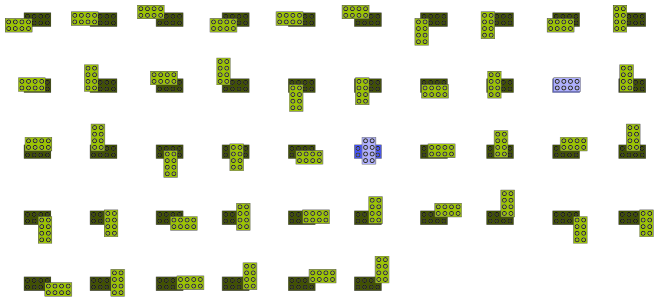
Figure 1: 46 basic positions

We consider contiguous buildings of LEGO blocks, disregarding color, and identify them up to translation and rotation. We think of a $b\times w$ LEGO block as a subset of $\mathbb{R}^{3}$ of the form

$$[x;x+b]\times[y,y+w]\times[z;z+1]$$

or

$$[x;x+w]\times[y,y+b]\times[z;z+1]$$

Since the top and bottom of a LEGO block are distinguishable we will only consider rotations in the $xy$-plane.

It is easy to see that one such block may be put on top of another in

$$(2b-1)(2w-1)+(b+w-1)^{2}$$ (1.1)

different ways if $b\not=w$ and in

$$(2b-1)^{2}$$ (1.2)

different ways if $b=w$.

With $w=4$ and $b=2$ we get $46$ possibilities, and note (as depicted in blue on Figure 1) that $2$ of these are symmetric. Thus, letting $H_{2\times 4}(n,m)$ denote the number of ways to build a building of height $m$ with $n$ $2\times 4$ LEGO blocks one then clearly has

$$H_{2\times 4}(n,n)=\frac{1}{2}(46^{n-1}+2^{n-1})$$

Note that $H_{2\times 4}(6,6)=102981504$, so that in fact LEGO’s computation is off by four.

By combining results of computer-aided enumerations with elementary combinatorics one can further establish

$$H_{2\times 4}(n,n-1)=46^{n-4}(-89115+37065n)+2^{n-4}(-8+16n)$$ (1.3)

for $n\geq 3$ and

$$H_{2\times 4}(n,n-2)=2^{n-7}(1785-825n+256n)$$ (1.4)

$$+46^{n-7}(-918674675-5330182078n+1373814225n^{2})$$

for $n\geq 5$, but as the problem is rather hopelessly non-markovian there seems to be no way to give formulae for the number of buildings of relatively low height, or indeed for the total number $T_{2\times 4}(n)$ of contiguous configurations, counted up to symmetry. Although symmetry arguments and other tricks can be used to prune the search trees somewhat, we are essentially left with the very time-consuming option of going through all possible configurations to determine these numbers, which even with efficient computers seems completely out of range for numbers such as $T_{2\times 4}(12)$. A sample of our results may be seen in Figure 2.

$H_{2\times 4}(n,m)$	$m=2$	$m=3$	$m=4$	$m=5$	$m=6$
$n=2$	24
$n=3$	500	1060
$n=4$	11707	59201	48672
$n=5$	248688	3203175	4425804	2238736
$n=6$	7946227	162216127	359949655	282010252	102981504

Figure 2: $H_{2\times 4}(n,m)$ for $m,n\leq 6$

These results seem to indicate, as shown on Figure 3, that $T_{2\times 4}(n)$ grows exponentially in $n$. In this paper we will show that this is indeed the case, and give upper and lower bounds on the rate of growth – the entropy of the blocks.

$n$	$T_{2\times 4}(n)$
1	1
2	24
3	1560
4	119580
5	10116403
6	915103765
7	85747377755

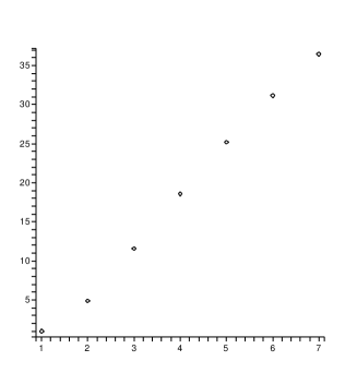
Figure 3: Rate of growth of $T_{2\times 4}$ with semilogarithmic plot

2 Entropy of $b\times w$ blocks

It is the goal of the present section to prove that the following definition makes sense:

Definition 2.1

The entropy of a $b\times w$ LEGO block is

$$s_{{b\times w}}=\lim_{n\longrightarrow\infty}\frac{\log(T_{b\times w}(n))}{n}$$ (2.5)

We let $h_{{b\times w}}=\exp(s_{b\times w})$.

That the limit exists is by no means obvious, except of course for $s_{1\times 1}=0$. We shall prove that this is the case in two steps, first establishing convergence in $[0;\infty]$ and then proving that the limit is finite.

It is inconvenient and irrelevant for our theoretical considerations to identify buildings up to symmetry, so we establish definiteness in another fashion. Suppressing the block size from the notation, we will by $\mathcal{A}_{n}$ denote all contiguous buildings containing $[0;w]\times[0;b]\times[0;1]$ with the further property that there is no other block in $\mathbb{R}^{2}\times[0;1]$ and no block at all in $\mathbb{R}^{2}\times[-1;0]$. Thus, the configuration can be thought of as sitting on a base block at a fixed position.

We let $\mathsf{a}_{n}=\#\mathcal{A}_{n}$ and note

Lemma 2.2

We have

$$\lim_{n\longrightarrow\infty}\frac{\log(T_{b\times w}(n))}{n}=\lim_{n\longrightarrow\infty}\frac{\log(\mathsf{a}_{n})}{n}$$

in the sense that if one limit exists, so does the other.

Proof: The claims follow immediately by the inequalities

$$T_{b\times w}(n-1)\leq\mathsf{a}_{n}\leq 4T_{b\times w}(n)$$

The leftmost inequality follows by mapping each equivalence class of configurations with $n-1$ blocks to a representative placed on top of $[0;w]\times[0;b]\times[0;1]$ and noting that this map is injective. The rightmost follows by mapping each configuration to an equivalence class and noting that this map is at most $4-1$. $\square$

We now get

Proposition 2.3

${\log(\mathsf{a}_{n})}/n$ converges in $[0;\infty]$ as $n\longrightarrow\infty$.

Proof: One sees that $\mathsf{a}_{n+m}\geq\mathsf{a}_{n}\mathsf{a}_{m}$ by noting that an injective map from $\mathcal{A}_{n}\times\mathcal{A}_{m}$ to $\mathcal{A}_{m+n}$ is defined by placing the base block of the element of $\mathcal{A}_{m}$ somewhere on the top layer of the element of $\mathcal{A}_{n}$.

Hence $\log(\mathsf{a}_{n})$ is a superadditive sequence, and $\log(\mathsf{a}_{n})/n$ converges to

$$\sup_{n\in\mathbb{N}}\log(\mathsf{a}_{n})/n.$$

$\square$

To prove that this limit is finite, i.e. that $\mathsf{a}_{n}$ grows no faster than exponentially, we describe a surjective map associating to each function

$$S_{n}:\{1,\dots,2bw(n-2)\}\longrightarrow\{-bw,-bw+1,\dots,bw-1,bw\}$$ (2.6)

an element of

$$\mathcal{A}_{n}\cup\{\mathsf{FAIL}\}.$$

Clearly the number of such functions grows only exponentially in $n$. We shall subsequently look closer at which functions do indeed lead to buildings with $n$ LEGO blocks, and give much better estimates for $h_{b\times w}$ than the obvious $(2bw+1)^{2bw}$.

With a fixed enumeration of the studs and holes of a $b\times w$ LEGO block by the numbers $1,\dots,bw$, a map of the form (2.6) gives rise to an element of $\mathcal{A}_{n}$, or the symbol $\mathsf{FAIL}$, as follows.

Take one LEGO block and call it block 1. Then read $S_{n}(1),\dots,S_{n}(bw)$ from left to right to specify what to build on top of block 1 as follows. If $S_{n}(1)>0$, take another LEGO block and place it parallely to block 1 with hole $S_{n}(1)$ on top of stud 1. If $S_{n}(1)<0$, take a LEGO block and place it orthogonally, rotated $+90^{\circ}$, to block 1 with hole $-S_{n}(1)$ on top of hole 1. In both cases, give the new block the number 2. If $S_{n}(1)=0$, do nothing. Then proceed to read $S_{n}(2)$ to see what, if anything, to place on stud 2, and so on until $S_{n}(bw)$. Enumerate the blocks as they are introduced.

Terminal state 2.4

If at any point a block collides with one which has already been placed, the procedure terminates with $\mathsf{FAIL}$.

These steps will result in the placing of between 0 and $bw$ blocks on block 1.

Terminal state 2.5

If at any point all $n$ blocks have been placed, consider the unread values of $S_{n}$. If they are all $0$, the procedure terminates successfully with an element of $\mathcal{A}_{n}$. If not, the procedure terminates with $\mathsf{FAIL}$.

Terminal state 2.6

If, after reading the specifications for the first $m<n-1$ blocks, no block $m+1$ has been introduced, the procedure terminates with $\mathsf{FAIL}$.

We may now assume that a block 2 has been introduced and look at $S_{n}(bw+1),\dots,S_{n}(2bw)$ which will specify what to build on top of this block, if anything, in the same way that $S_{n}(1),\dots,S_{n}(bw)$ specified what to build on block 1. A positive number at $S_{n}(bw+1)$ will result in the placing of a block on stud 1 of block 2 parallel to block 1, a negative number at $S_{n}(bw+1)$ will result in the placing of a block on stud 1 of block 2 orthogonal to block 1, etc. We proceed in the same way for blocks $3,\dots,n-1$, but now read $2bw$ values where $S_{n}((2m-4)bw+1),\dots,S_{n}((2m-3)bw)$ will specify what to put on top of block $m$, and $S_{n}((2m-3)bw+1),\dots,S_{n}((2m-2)bw)$ will specify what to put on underneath it in an analogous way.

Terminal state 2.7

If at any point a second block is placed at the level $\mathbb{R}^{2}\times[0;1]$, the procedure terminates with $\mathsf{FAIL}$.

Terminal state 2.8

If $S_{n}$ has been read to the end, consider the number of blocks placed. If it is less than $n$, the procedure terminates with $\mathsf{FAIL}$. If not, it terminates successfully with an element of $\mathcal{A}_{n}$.

We repeat this until one of the terminal states are reached.

If the procedure does not fail, it will result in a building of $n$ contiguous blocks, and clearly any such building may be constructed in this way. Thus, the number of possibilites for maps $S_{n}$ dominates $\mathsf{a}_{n}$, as desired, and we have:

Theorem 2.9

The limit in (2.5) exists for any block dimension $b\times w$.

We can give general bounds of $h_{b\times w}$, but as wee shall see below in the case $w=4,b=2$, these bounds can in general be rather dramatically improved.

Theorem 2.10

If $b\not=w$ we have

$$(2b-1)(2w-1)+(b+w-1)^{2}\leq h_{b\times w}\leq\frac{(2bw)^{2bw+1}}{(2bw-1)^{2bw-1}}$$ (2.7)

If $b=w$ we have

$$(2b-1)^{2}\leq h_{b\times w}\leq\frac{(b^{2})^{2b^{2}+1}}{(b^{2}-1)^{2b^{2}-1}}$$ (2.8)

Proof: By (1.1) we clearly have

$$\mathsf{a}_{n}\geq((2b-1)(2w-1)+(b+w-1)^{2})^{n-1}$$

when $b\not=w$, and this gives the lower bound in that case. For the upper bound, note that a function $S_{n}$ with nonzero entries at $m$ locations will yield $\mathsf{FAIL}$ if $m\not=n-1$. Hence we get

$$\mathsf{a}_{n}\leq\left(\begin{array}[]{c}2bw(n-2)\\ n-1\end{array}\right)(2bw)^{n-1}$$

By Stirling’s formula we then get

$$\mathsf{a}_{n} \leq \frac{(2bw(n-2))!}{(n-1)!((2bw-1)n-4bw+1)!}(2bw)^{n-1}$$

$$= \frac{(2bwn)!(2bw)^{n}}{n!((2bw-1)n)!}O(1)$$

$$= \frac{(2bwn)^{2bwn}(2bw)^{n}}{n^{n}((2bw-1)n)^{(2bw-1)n}}O(n^{-1/2})$$

$$= \frac{(2bw)^{2bwn}(2bw)^{n}}{(2bw-1)^{(2bw-1)n}}O(n^{-1/2})$$

$$= \left(\frac{(2bw)^{2bw+1}}{(2bw-1)^{2bw-1}}\right)^{n}O(n^{-1/2})$$

from which the claim follows directly.

The square case follows similarly by (1.2) and by noting that functions $S_{n}$ may be chosen non-negative. $\square$

Example 2.11

We enumerate the studs of a $2\times 4$ LEGO block according to Figure 4.

1 2 3 4

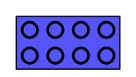
5 6 7 8

Figure 4: Enumeration of studs and holes

Now consider functions $\{1,\dots,32\}\mapsto\{-8,\dots,8\}$ given by

$$(\overbrace{0,5,0,0,-4,0,0,0}^{1},\overbrace{0,0,0,0,-1,0,0,0}^{2},\overbrace{0,\dots,0,0,\dots,0}^{3})$$ (2.9)

$$(\overbrace{0,-1,0,0,0,0,0,0}^{1},\overbrace{0,5,0,0,0,0,0,0}^{2},\overbrace{0,\dots,0,0,0,0,-1,0,0,0}^{3})$$ (2.10)

$$(\overbrace{1,1,0,0,0,0,0,0}^{1},\overbrace{0,\dots,0}^{2},\overbrace{0,\dots,0,0,\dots,0}^{3})$$ (2.11)

$$(\overbrace{0,-1,0,0,0,0,0,0}^{1},\overbrace{0,5,0,0,0,0,0,0}^{2},\overbrace{0,\dots,0,0,0,0,-1,0,-1,0}^{3})$$ (2.12)

$$(\overbrace{0,\dots,0}^{1},\overbrace{0,\dots,0}^{2},\overbrace{0,\dots,0,0,\dots,0}^{3})$$ (2.13)

$$(\overbrace{0,-1,0,-1,0,0,0,0}^{1},\overbrace{0,\dots,0}^{2},\overbrace{0,0,2,0,0,0,0,0,\dots,0}^{3})$$ (2.14)

$$(\overbrace{0,-1,0,0,0,0,0,0}^{1},\overbrace{0,5,0,0,0,0,0,0}^{2},\overbrace{0,\dots,0,0,\dots,0}^{3})$$ (2.15)

where all ellipses indicate six consecutive zeros. The functions (2.9) and (2.10) give rise to the buildings depicted on Figure 5.

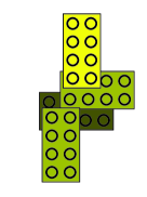
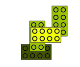
Figure 5: Buildings associated to (2.9) and (2.10)

The remaining five functions give simple examples of functions resulting in the procedure failing at Terminal state 2.4, 2.5, 2.6, 2.7, and 2.8, respectively.

3 Improved upper bounds

In this section we shall describe methods to improve the upper bound on $h_{b\times w}$ given in Theorem 2.10. They apply to any dimension, but as they are somewhat ad hoc we shall concentrate on our favored dimension $2\times 4$ and leave other cases to the reader.

From Theorem 2.10 we know that $h_{2\times 4}\leq 16^{17}/15^{15}\leq 647.02$. We shall give a simple improved estimate leading to $h_{2\times 4}\leq 203.82$ and a somewhat more complicated one leading to $h_{2\times 4}\leq 191.35$. Besides being easier to state, the simpler estimate has applications in producing statistical estimates for $\mathsf{a}_{n}$ for relatively large $n$.

Note that the surjective map associating buildings (or $\mathsf{FAIL}$) to certain maps

$$S_{n}:\{1,\dots,16(n-2)\}\longrightarrow\{-8,-7,\dots,7,8\}$$

is very far from being injective. We have already employed the fact that unless the number of nonzero values is $n-1$, the function is mapped to $\mathsf{FAIL}$. But we may also use that the placement of a block onto another may be indicated in $\ell$ different ways, where $\ell$ is the number of studs of the lower block which are inserted into the upper block. Restricting attention to maps where placements are indicated in a fixed way will not affect surjectivity of the map.

Any partition of the 46 positions in Figure 1 into 8 sets $\mathcal{P}_{1},\dots,\mathcal{P}_{8}$ with the property that any position in $\mathcal{P}_{i}$ employs stud $i$ of the lower block can be used to improve the upper bound. One uses the convention that a position in $\mathcal{P}_{i}$ is always indicated by a symbol at stud $i$, thus restricting the number of possibilities.

Another restriction is available when specifying what to add to block $m$ for $m>2$. If we keep track of how block $m$ was introduced, we know a priori that one hole or one stud of it has already been used, thus eliminating at least $16$ out of the $46$ possibilities on the relevant side of the block. Dividing up the remaining 30 positions as above, we get 64 sets $\mathcal{P}^{j}_{i}$ with the property that $\mathcal{P}^{i}_{i}=\emptyset$ and that $\mathcal{P}^{j}_{1},\dots,\mathcal{P}^{j}_{8}$ is a partition of the 30 positions which do not employ stud $j$.

Theorem 3.1

We have

$$\mathsf{a}_{n}\leq\left(\begin{array}[]{c}13n-23\\ n-1\end{array}\right)6^{n-1}$$ (3.18)

and, consequently, that $h_{2\times 4}\leq 6\cdot 13^{13}/12^{12}<203.82$

Proof: We partition the 46 positions into 8 sets, each consisting of 6 or 5 configurations, as indicated by the rows of Figure 6. Thus on indices related to one side of blocks $1,\dots,n-1$, we need only allow for 6 different symbols.

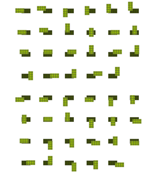
Figure 6: Even distribution

On the other side of blocks $3,\dots,n-1$, we can do even better, as outlined above. We leave to the reader to check that the 30 positions may be distributed evenly over 5 studs. Hence, (3.18) is established, and the remaining claim follows by Stirling’s formula as in Theorem 2.10. $\square$

It turns out – somewhat counterintuitively? – that uneven distributions of the positions give slightly better estimates than what we obtained above. We have not carried out a systematic analysis and can not claim that the distribution leading to Theorem 3.3 is optimal, but trial and error with the following proposition make us believe that there is only marginal room for improvement by this method.

If $(a_{1},\dots,a_{8})$ and $(b_{1},\dots,b_{8})$ are tuples of integers, we write $(a_{1},\dots,a_{8})\leq(b_{1},\dots,b_{8})$ if there is a permutation $\sigma$ of $\{1,\dots,8\}$ with the property that $a_{\sigma(i)}\leq b_{i}$ for each $i$.

The methods leading to the following result are surely known.

Proposition 3.2

Let $\mathcal{P}_{i}$ and $\mathcal{P}^{j}_{i}$ be partitions of the sets of positions as outlined above, and assume that

$$(\#\mathcal{P}_{1},\dots,\#\mathcal{P}_{8})\leq(a_{1},\dots,a_{8})$$

$$(\#\mathcal{P}^{j}_{1},\dots,\#\mathcal{P}^{j}_{8})\leq(b_{1},\dots,b_{8}),\qquad j\in\{1,\dots,8\}.$$

With

$${P}_{0}(y)=(y+a_{1})\cdots(y+a_{8})\qquad P(y)={P}_{0}(y)(y+b_{1})\cdots(y+b_{8})$$

we have that $\mathsf{a}_{n}$ is dominated by the coefficient of $y^{15n-31}$ in $({P}_{0}(y))^{2}(P(y))^{n-3}$ and that

$$h_{2\times 4}\leq\frac{P(x_{0})}{x_{0}^{15}}$$

where $x_{0}$ is the largest real root of

$$Q(x)=15P(x)-xP^{\prime}(x)$$

With the even distribution described above we get $x_{0}=72$, which, since $P(72)/72^{15}=6\cdot 13^{13}/12^{12}$ is consistent with Theorem 3.1. Using that in fact $(\#\mathcal{P}_{1},\dots,\#\mathcal{P}_{8})\leq(5,5,6,6,6,6,6,6)$ we may improve the estimate on $h_{2\times 4}$ sligthly to $198.57$.

However, we can do even better with very uneven distributions:

Theorem 3.3

$h_{2\times 4}\leq 191.35$

Proof: There exist partitions with

$$(\#\mathcal{P}_{1},\dots,\#\mathcal{P}_{8})\leq(16,15,7,5,2,1,0,0)$$

$$(\#\mathcal{P}^{j}_{1},\dots,\#\mathcal{P}^{j}_{8})\leq(15,7,4,3,1,0,0,0),\qquad j\in\{1,\dots,8\}.$$

so by Proposition 3.2 we are lead to consider

$$P(x)=-x^{5}(x+15)(x+7)(x+1)R(x)$$

where $R(x)$ is the polynomial

$$x^{8}-23x^{7}-2056x^{6}-38700x^{5}-332657x^{4}-1504645x^{3}-3645736x^{2}-4392600x-2016000$$

which has a largest real root which is approximately $65.05$. The estimate follows by Proposition 3.2. $\square$

4 Improved lower bounds

It follows from Theorem 2.10 that $h_{2\times 4}\geq 46$. We shall in this section improve this estimate to $h_{2\times 4}>78.32$.

We let $\mathcal{B}_{n}\subset\mathcal{A}_{n+1}$ denote the set of LEGO configurations as above consisting of $n+1$ blocks and such that both the top and the bottom layer consists of a single block. Setting $\mathsf{b}_{n}=\#\mathcal{B}_{n}$ we then clearly have

$$\mathsf{a}_{n}\leq\mathsf{b}_{n}\leq\mathsf{a}_{n+1}$$

and hence, as in Lemma 2.2,

$$h_{2\times 4}=\exp\left(\lim_{n\longrightarrow\infty}\frac{\log\mathsf{b}_{n}}{n}\right).$$ (4.19)

We say that a configuration $c$ in $\mathcal{B}_{n}$ has a bottleneck at height $z\in\mathbb{N}$ if $c$ has exactly one block in the layer $\mathbb{R}^{2}\times[z;z+1]$. By convention the top and bottom blocks are not bottlenecks. This ensures that removal of a bottleneck decomposes $c$ into two configurations $c_{0}^{\prime}$ and $c_{0}^{\prime\prime}$ one of which, say $c_{0}^{\prime}$, contains the bottom block of $c$. Re-inserting the removed block in $c_{0}^{\prime}$ yields a configuration $c^{\prime}$ in some $\mathcal{B}_{n}$ with the inserted block as the top block. Re-inserting the removed block into $c_{0}^{\prime\prime}$ yields, after a translation, a configuration $c^{\prime\prime}$ in $\mathcal{B}_{n-m}$ with the inserted block (translated) as the bottom block. Evidently, we can reconstruct $c$ in a unique fashion from $(c^{\prime},c^{\prime\prime})$. Repeating this decomposition procedure we conclude that any configuration in $\mathcal{B}_{n}$ with exactly $k\geq 0$ bottlenecks can in a unique way be decomposed into a sequence $(c^{(1)},\dots,c^{(k+1)})$ of configurations such that $c^{(i)}\in\mathcal{B}_{m_{i}}$ has no bottlenecks and $m_{1}+\dots+m_{k+1}=n$.

Figure 7: Two bottlenecks

Letting $\mathcal{C}_{n}$ denote the subset of $\mathcal{B}_{n}$ consisting of configurations without bottlenecks we obtain in this way a one-to-one correspondence between elements of $\mathcal{B}_{n}$ and those of

$$\bigcup_{k=0}^{\infty}\left[\bigcup_{m_{1}+\dots+m_{k+1}=n}\mathcal{C}_{m_{1}}\times\cdots\times\mathcal{C}_{m_{k+1}}\right]$$ (4.20)

Let now

$$\mathsf{c}_{n}=\#\mathcal{C}_{n}$$

and let $\psi$ and $\psi_{0}$ denote the generating functions

$$\psi(z)=\sum_{n=1}^{\infty}\mathsf{b}_{n}z^{n}\qquad\psi_{0}(z)=\sum_{n=1}^{\infty}\mathsf{c}_{n}z^{n}$$ (4.21)

It follows from (4.20) that

$$\psi(z)=\sum_{i=1}^{\infty}(\psi_{0}(z))^{i}=\frac{\psi_{0}(z)}{1-\psi_{0}(z)}.$$ (4.22)

From the definition of $\psi(z)$ and $h_{2\times 4}$ it follows that $\psi$ is analytic in the disc

$$D=\{z\mid|z|<(h_{2\times 4})^{-1}\}$$

and, since $b_{n}>0$, that $\psi$ is non-analytic at $z=(h_{2\times 4})^{-1}$. From (4.22) we hence conclude that

$$|\psi_{0}(z)|<1\qquad\text{ for }|z|<(h_{2\times 4})^{-1}$$ (4.23)

In particular, we get

$$\mathsf{c}_{1}(h_{2\times 4})^{-1}+\cdots+\mathsf{c}_{n}(h_{2\times 4})^{-n}\leq 1$$

which gives our claimed lower bounds on $h_{2\times 4}$, depending on the number of terms $n$ on the lefthand side.

We shall describe in detail how to get the first order of improvement of the estimate from Theorem 2.10. As evidently $\mathsf{c}_{2}=0$ we turn to $\mathsf{c}_{3}$ for this.

The configurations contributing to $\mathsf{c}_{3}$ have one bottom block, one top block. and two blocks in between. The number of ways of placing two blocks on top of the bottom block is rather easily seen to be $480$, so the number of configurations where the two middle blocks are both attached to the bottom block is $2\cdot 46\cdot 480-4730$, where $4730$ is the number of configurations where the middle blocks are both attached to the top block as well as to the bottom block. The remaining configurations are those where the middle blocks are both attached to the top block but only one of them to the bottom. This number is seen to be $2\cdot 46\cdot 480-2\cdot 4730$. Thus we have

$$\mathsf{c}_{3}=4\cdot 46\cdot 480-3\cdot 4730=74130$$

and $P_{3}(h_{2\times 4}^{-1})\leq 1$ where

$$P_{3}(x)=46x+{74130}x^{3}$$

This gives

$$h_{2\times 4}\geq 64.06$$

which can be improved as follows.

Theorem 4.1

$h_{2\times 4}>78.32$

Proof: Computer-aided computations give

$$\mathsf{c}_{4} = 867346$$

$$\mathsf{c}_{5} = 318434429$$

$$\mathsf{c}_{6} = 18335373238$$

so we have that $P_{6}(h_{2\times 4}^{-1})\leq 1$ where

$$P_{6}(x)=46x+{74130}x^{3}+{867346}x^{4}+{318434429}x^{5}+{18335373238}x^{6}$$

which gives $h_{2\times 4}>76.67$.

To improve the estimate we prove that

$$\mathsf{c}_{n+2}\geq 1248\mathsf{c}_{n}$$ (4.24)

for $n\geq 6$. To see this, we devise 1248 different ways to construct an element $c^{\prime}$ of $\mathcal{C}_{n+2}$ from an element $c$ of $\mathcal{C}_{n}$, in such a way that the original configuration can be recovered from the resulting one.

Of these 1248 configurations, 480 are gotten from a fixed configuration $d$ of two blocks sitting on one base block $b$ by identifying the base block of $c$ with the block at the second level of $d$ which meets the stud of lowest index on $b$ according to the enumeration of Figure 4. We get the configuration $c^{\prime}$ by rotating 90^∘, if necessary. The remaining 768 configurations are gotten by placing one block underneath the base block of $c$, and placing one more block at the level of this original base block, such that these two added blocks do not meet. A computer search shows that there is always at least this number of ways to do so since there are at least two blocks at level $1$ of $c$ but only one at level $0$. We get the configuration $c^{\prime}$ by translating the configuration upwards and rotating 90^∘, if necessary.

To reconstruct $c$ from $c^{\prime}$, one first sees how many blocks are attached to the base block of $c^{\prime}$. If there are two, $c$ is gotten by discarding the base block of $c^{\prime}$ and the block at the next level sitting at the highest index of it, translating down and rotating $270^{\circ}$, if necessary. If there is only one, $c$ is gotten by discarding the base block of $c^{\prime}$ and the block at the next level which does not meet that block, translating down and rotating $270^{\circ}$, if necessary.

By repeated application of (4.24) we get $\mathsf{c}_{6+2k}\geq 1248^{k}\mathsf{c}_{6}$ and $\mathsf{c}_{5+2k}\geq 1248^{k}\mathsf{c}_{5}$, so that $r(h_{{2\times 4}})\leq 1$ with

$$r(x)=P_{6}(x)+\frac{\mathsf{c}_{5}x^{7}+\mathsf{c}_{6}x^{8}}{1/1248-x^{2}},$$

leading to the stated lower bound. $\square$

5 Concluding remarks

We do not at present have the software nor the computer power to perform numerical experiments to get a good idea of the true value of $h_{{2\times 4}}$. Our best guess, based mainly on data achieved by Abrahamsen on the presumably closely related case of $1\times 2$-blocks would be that the number is rather close to $100$.

Department of Mathematics
University of Copenhagen
Universitetsparken 5
DK-2100 Copenhagen Ø
Denmark

References

- [1] Mikkel Abrahamsen, LEGO counting results. Odsherreds Gymnasium.
- [2] Jørgen Kirk Christiansen, ”Taljonglering med klodser – eller talrige klodser. Klodshans (LEGO Company newsletter), 1974.
- [3] Kjeld Kirk Christiansen, The ultimate LEGO book. Dorling Kindersley, 1999.
- [4] LEGO Company Profile 2004, LEGO, http://www.lego.com/info/pdf/compprofileeng.pdf.
- [5] Trine Nissen, From 102 to 915 million combinations LEGOLife 5, Company newsletter, 2004. Available from http://www.math.ku.dk/~eilers/lego.html.