Exact Polynomial Eigenmodes for Homogeneous Spherical 3-Manifolds

Abstract

Observational data hint at a finite universe, with spherical manifolds such as the Poincaré dodecahedral space tentatively providing the best fit. Simulating the physics of a model universe requires knowing the eigenmodes of the Laplace operator on the space. The present article provides explicit polynomial eigenmodes for all globally homogeneous 3-manifolds: the Poincaré dodecahedral space $S^{3}/I^{*}$, the binary octahedral space $S^{3}/O^{*}$, the binary tetrahedral space $S^{3}/T^{*}$, the prism manifolds $S^{3}/D_{m}^{*}$ and the lens spaces $L(p,1)$.

1 Introduction

The past decade has seen intense work on multiconnected 3-manifolds as models for the physical universe. Well-proportioned 3-manifolds explain the missing broad-scale fluctuations in the cosmic microwave background, first discovered by the COBE satellite [1] and later confirmed by the WMAP satellite [2, 3]. (Please see Ref. [4] for an elementary exposition.) A well-proportioned 3-manifold is one whose three dimensions are of comparable magnitudes. Ill-proportioned manifolds, with one dimension significantly larger or smaller than the other two, fail to explain the missing broad-scale fluctuations and indeed predict exactly the opposite, namely elevated broad-scale fluctuations [5], contrary to observations. Current work, therefore, focuses on well-proportioned spaces.

The density of ordinary matter alone would suggest a hyperbolic universe, and so ten years ago researchers studied hyperbolic models. The situation changed dramatically in late 1998 with the discovery of a still-mysterious vacuum energy that raises the universe’s mass-energy density parameter $\Omega$ to the level required for a flat space ($\Omega=1$) or a slightly spherical space ($\Omega>1$). The first-year WMAP paper [2] put $\Omega$ at $1.02\pm 0.02$ at the $1\sigma$ level, while the three-year WMAP paper [3] reports six different distributions ranging from a rather flat $\Omega=1.003^{+0.017}_{-0.013}$ to a surprisingly curved $\Omega=1.037^{+0.015}_{-0.021}$ depending on what external data set one uses to resolve the geometrical degeneracy.

The Poincaré dodecahedral space [6], defined as the quotient $S^{3}/I^{*}$ of the 3-sphere by the binary icosahedral group $I^{*}$, explains both the missing fluctuations and the observed mass-energy density [7] and so researchers are now modelling it more precisely for better comparison to observations. State-of-the-art simulations find that the Poincaré dodecahedral space matches observed broad-scale fluctuations when $1.015<\Omega<1.020$ [8, 9] or $1.022<\Omega<1.034$ [10], in excellent agreement with the three-year WMAP estimates of $\Omega$. However, other topologies, notably the quotient $S^{3}/O^{*}$ of the 3-sphere modulo the binary octahedral group, also remain viable [9, 10].

Attempts to confirm a multiconnected universe using the circles-in-the-sky method [11] have failed [12]. (Exception: one research group claims to have found hints of matching circles [13] and a second group has confirmed the match [14], but the former provide no statistical analysis while the latter find the match to lie below the false positive threshold, so the former’s claim remains unconvincing.) Accepting the result that any potential circle pairs are undetectable [12], the question remains: are the circles really not there, or are they merely hidden by various sources of contamination, such as the Doppler and integrated Sachs-Wolfe components of the microwave background? Answering this question requires great care, because the level of contamination depends both on the topology and on the choice of cosmological parameters. Results so far remain inconsistent: the circle-searchers’ own analysis finds their negative results to be robust for a dodecahedral universe in spite of the contamination [14], while other researchers find contamination strong enough to hide matching circles [15].

To determine the observational consequences of a given cosmological model, researchers take a Fourier approach and express physical quantities, such as density fluctuations in the primordial plasma, as linear combinations of the eigenmodes of the Laplacian (more briefly, the modes), which can then be integrated forward in time. Thus all studies of cosmic topology require knowing the modes of the 3-manifold under consideration. Different research groups have determined the modes in different ways [8, 9, 10, 16, 17], but so far all approaches have required some sort of numerical computation, either the extraction of the eigenvectors of a large matrix or the solution of a large set of simultaneous equations.

The present article provides the modes as explicit polynomials with integer coefficients. That is, for each manifold $S^{3}/\Gamma$ and each wavenumber $k$, we provide a finite set of $\Gamma$-invariant polynomials of degree $k$ spanning the full space of modes. We provide these polynomials for the binary icosahedral space $S^{3}/I^{*}$ (better known as the Poincaré dodecahedral space), the binary octahedral space $S^{3}/O^{*}$, the binary tetrahedral space $S^{3}/T^{*}$, the binary dihedral spaces $S^{3}/D_{m}^{*}$ (better known as prism manifolds), the homogeneous lens spaces $L(p,1)$, and the 3-sphere itself. These spaces comprise the full set of globally homogeneous spherical 3-manifolds (called single action spaces in the classification of Ref. [18]).

The ideas in the present article draw heavily on Klein’s 1884 Vorlesungen über das Ikosaeder [19], extending Klein’s work to produce full bases of explicit polynomials.

Sections 2 through 9 are elementary in nature, laying a foundation, establishing terminology, and translating into geometric language some concepts that have recently appeared in the cosmic topology literature only in quantum mechanical bracket language. Sections 10 through 15 provide the real content of this article, namely the explicit polynomials for the modes of $S^{3}/I^{*}$, $S^{3}/O^{*}$, $S^{3}/T^{*}$, $S^{3}/D_{m}^{*}$, $L(p,1)$ and $S^{3}$. Section 16 outlines future work.

2 Lifting $S^{2}$ to $S^{3}$

Let us parameterize the 2-sphere $S^{2}$ first as the Riemann sphere $\mathbb{C}\cup\{\infty\}$ and then, more elegantly, as the complex projective line $\mathbb{C}P^{1}$. First map the unit 2-sphere onto the equatorial plane via stereographic projection from the south pole: typical points map via $(x,y,z)\mapsto\frac{x}{z+1}+i\frac{y}{z+1}$ while the south pole $(0,0,-1)$ maps to $\infty$. To accommodate the south pole into the same format as the typical points, write each image point as a formal fraction. Each typical point maps to a formal fraction $\frac{x+iy}{z+1}$, while the south pole maps to the formal fraction $\frac{1}{0}$. Two formal fractions $\frac{\alpha}{\beta}$ and $\frac{\alpha^{\prime}}{\beta^{\prime}}$ are equivalent if and only if $\alpha\beta^{\prime}=\alpha^{\prime}\beta$. Let $[\frac{\alpha}{\beta}]$ denote the equivalence class of all formal fractions $\frac{\alpha^{\prime}}{\beta^{\prime}}$ equivalent to $\frac{\alpha}{\beta}$. The set of all such equivalence classes defines the complex projective line $\mathbb{C}P^{1}$. The indeterminate fraction $\frac{0}{0}$ is of course excluded from the discussion. In summary, the set $\mathbb{C}P^{1}$ of equivalence classes $[\frac{\alpha}{\beta}]$ of of nontrivial complex formal fractions parameterizes the 2-sphere $S^{2}$.

Writing the formal fraction $\frac{\alpha}{\beta}$ as an ordered pair $(\alpha,\beta)\in\mathbb{C}^{2}$ immediately yields a map $\mathbb{C}^{2}-(0,0)\rightarrow\mathbb{C}P^{1}$ sending each point $(\alpha,\beta)\in\mathbb{C}^{2}$ to the corresponding equivalence class $[\frac{\alpha}{\beta}]\in\mathbb{C}P^{1}$. The radial direction in $\mathbb{C}^{2}$ is largely irrelevant, because $(\alpha,\beta)$ and $(r\alpha,r\beta)$ map to the same class $[\frac{\alpha}{\beta}]=[\frac{r\alpha}{r\beta}]\in\mathbb{C}P^{1}$ for all real $r\neq 0$. We may therefore restrict the map’s domain to the unit 3-sphere $S^{3}\subset\mathbb{C}^{2}$ without compromising its image in $\mathbb{C}P^{1}$. Recalling from the preceding paragraph that $\mathbb{C}P^{1}$ parameterizes $S^{2}$, this yields a map $S^{3}\rightarrow S^{2}$.

The Clifford flow  on $S^{3}\subset\mathbb{C}^{2}$ is the fixed-point-free motion taking $(\alpha,\beta)\mapsto(e^{it}\alpha,e^{it}\beta)$ for $0\leq t\leq 2\pi$. Under the Clifford flow, each point $(\alpha,\beta)$ traces out a great circle, which collectively form a set of Clifford parallels. The points along a given Clifford parallel all map to the same equivalence class $[\frac{e^{it}\alpha}{e^{it}\beta}]=[\frac{\alpha}{\beta}]\in\mathbb{C}P^{1}$. In other words, the preimage of each point of $S^{2}$ is a Clifford parallel in $S^{3}$ which we will call a fiber of the map.

3 Constructing the Groups

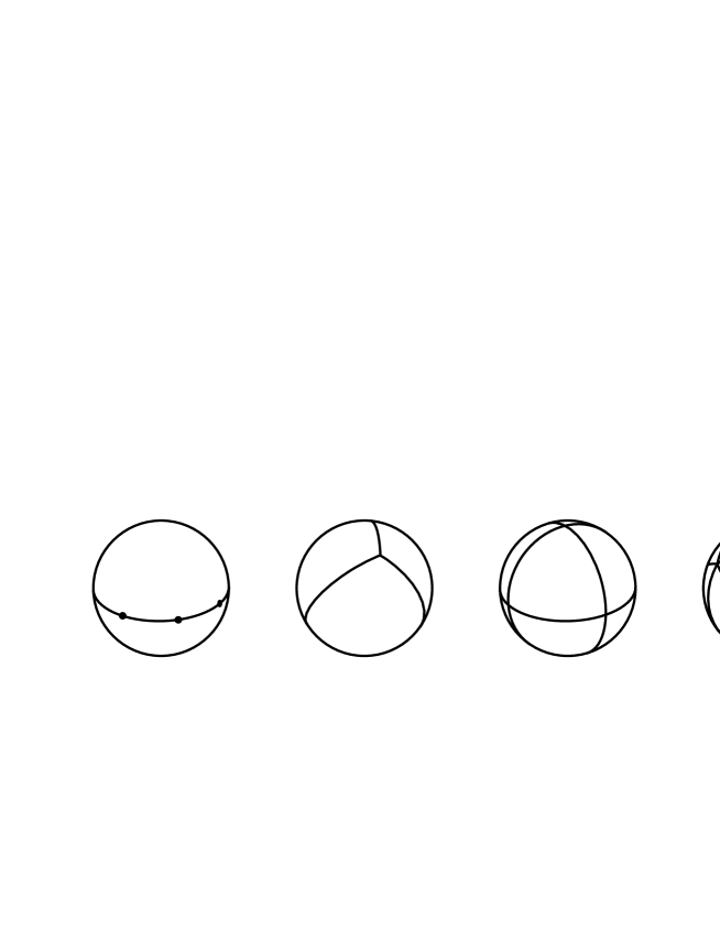
Figure 1: The dihedron, tetrahedron, octahedron and icosahedron project radially to tilings of the 2-sphere. The dihedron has only two faces, one filling the whole northern hemisphere and the other filling the whole southern hemisphere. The dihedron’s vertices and edges lie evenly along the equator. (Artwork by Adam Weeks Marano.)

The classic platonic solids project radially to tilings of $S^{2}$ (Figure 1). We ignore the cube and dodecahedron, because they are dual to the octahedron and icosahedron respectively, but include the dihedron, which works out fine as a tiling of $S^{2}$ even though it falls flat as a traditional polyhedron. The orientation-preserving symmetries of these tilings comprise the dihedral group $D_{m}$, the tetrahedral group $T$, the octahedral group $O$ and the icosahedral group $I$, of order $2m$, 12, 24 and 60, respectively.

Every matrix $(\phantom{|}^{a}_{c}\phantom{|}{}^{b}_{d}\phantom{|})\in GL_{2}\mathbb{C}$ respects Clifford parallels in the sense that left-multiplication takes each fiber $(e^{it}\alpha,e^{it}\beta)$ to another fiber $(e^{it}(a\alpha+b\beta),e^{it}(c\alpha+d\beta))$. Therefore the matrix action projects down to a well-defined map $S^{2}\rightarrow S^{2}$ taking $[\frac{\alpha}{\beta}]$ to $[\frac{a\alpha+b\beta}{c\alpha+d\beta}]$. Restricting our attention to unitary matrices $(\phantom{|}^{a}_{c}\phantom{|}{}^{b}_{d}\phantom{|})\in U(2)$ ensures rigid motions of $\mathbb{C}^{2}$, which in turn project down to rigid motions of $S^{2}$. The unitary matrices, however, still allow room for “sliding along the fibers”, for example via the matrix $(\phantom{|}^{e^{i\theta}}_{0}\phantom{|}{}^{0}_{e^{i\theta}}\phantom{|})$, which of course has no effect when projected down to $S^{2}$. To obtain an (almost) unique matrix for each rotation of $S^{2}$, restrict to the special unitary group $SU(2)$, whose matrices take the form $(\phantom{|}^{z}_{w}\phantom{|}{}^{-\bar{w}}_{\phantom{-}\bar{z}}\phantom{|})$. Each rotation of $S^{2}$ is realized by exactly two special unitary matrices $\pm(\phantom{|}^{z}_{w}\phantom{|}{}^{-\bar{w}}_{\phantom{-}\bar{z}}\phantom{|})$.

How may we construct the pair of matrices $\pm(\phantom{|}^{z}_{w}\phantom{|}{}^{-\bar{w}}_{\phantom{-}\bar{z}}\phantom{|})$ realizing a given rotation of $S^{2}$? To construct an order $n$ rotation about a desired fixed point $[\frac{p}{q}]$, we require that

$$\left(\begin{array}[]{cc}z&-\bar{w}\\ w&\phantom{-}\bar{z}\\ \end{array}\right)\left(\begin{array}[]{c}p\\ q\\ \end{array}\right)=\left(\begin{array}[]{c}e^{\frac{i\pi}{n}}p\\ e^{\frac{i\pi}{n}}q\\ \end{array}\right).$$ (1)

The phase factor $e^{\frac{i\pi}{n}}$ ensures that we rotate the correct amount about the given fixed point, so the isometry will have the desired order $n$. A quick calculation gives

$$\left(\begin{array}[]{c}z\\ \bar{w}\\ \end{array}\right)=\pm\frac{1}{p\bar{p}+q\bar{q}}\left(\begin{array}[]{cc}\phantom{-}\bar{p}&q\\ -\bar{q}&p\\ \end{array}\right)\left(\begin{array}[]{c}e^{\frac{+i\pi}{n}}p\\ e^{\frac{-i\pi}{n}}\bar{q}\\ \end{array}\right)$$ (2)

and $\pm(\phantom{|}^{z}_{w}\phantom{|}{}^{-\bar{w}}_{\phantom{-}\bar{z}}\phantom{|})$ follows immediately.

center	order	matrices
-	1	$\pm\left(\begin{array}[]{cc}1&\phantom{-}0\\ 0&\phantom{-}1\\ \end{array}\right)$
$0,\infty$	2	$\pm\left(\begin{array}[]{cc}i&\phantom{-}0\\ 0&-i\\ \end{array}\right)$
$\pm 1$	2	$\pm\left(\begin{array}[]{cc}0&\phantom{-}i\\ i&\phantom{-}0\\ \end{array}\right)$
$\pm i$	2	$\pm\left(\begin{array}[]{cc}0&-1\\ 1&\phantom{-}0\\ \end{array}\right)$

Table 1: The four rotations in $D_{2}\subset SO(3)$ correspond to eight matrices in $D_{2}^{*}\subset SU(2)$.

Equation (2) makes it easy to write down matrices for the groups $D_{m}$, $T$, $O$ and $I$. Two matrices realize each rotation of $S^{2}$, so for example the 4-element group $D_{2}\subset SO(3)$ is realized by an 8-element matrix group $D_{2}^{*}\subset SU(2)$ called the binary dihedral group of order 8 (Table 1). One might hope to extract a 4-element subgroup of $D_{2}^{*}$ realizing $D_{2}$ directly, but this is impossible because squaring an element of order 2 always gives $(\phantom{|}^{-1}_{\phantom{-}0}\phantom{|}{}^{\phantom{-}0}_{-1}\phantom{|})$, never $(\phantom{|}^{1}_{0}\phantom{|}{}^{0}_{1}\phantom{|})$, and once $(\phantom{|}^{-1}_{\phantom{-}0}\phantom{|}{}^{\phantom{-}0}_{-1}\phantom{|})$ is in a subgroup, so is the negative of every matrix in that subgroup.

Still using Equation (2), one may easily write down matrices for the 12-element tetrahedral group $T\subset SO(3)$, giving the 24-element binary tetrahedral group $T^{*}\subset SU(2)$, and similarly for the 48-element binary octahedral group $O^{*}$ and the 120-element binary icosahedral group $I^{*}$. The quotient $S^{3}/I^{*}$ defines the Poincaré dodecahedral space.

4 Constructing Symmetric Polynomials

Parameterize the 2-sphere $S^{2}$ as $\mathbb{C}P^{1}$ (Section 2) and let $P=\{[\frac{p_{1}}{q_{1}}],\dots,[\frac{p_{n}}{q_{n}}]\}$ be a set of points thereon, whose symmetry we hope to capture in a polynomial. As a starting point, the polynomial

$$(z-\frac{p_{1}}{q_{1}})\cdots(z-\frac{p_{n}}{q_{n}})$$ (3)

has roots exactly at $P$. Replacing the variable $z$ with a formal fraction $[\frac{\alpha}{\beta}]\in\mathbb{C}P^{1}$ gives

$$(\frac{\alpha}{\beta}-\frac{p_{1}}{q_{1}})\cdots(\frac{\alpha}{\beta}-\frac{p_{n}}{q_{n}})$$ (4)

which Klein, in his 1884 Vorlesungen über das Ikosaeder [19], writes as a homogeneous polynomial

$$(q_{1}\alpha-p_{1}\beta)\cdots(q_{n}\alpha-p_{n}\beta).$$ (5)

I thank Peter Kramer for his recent article [20] pointing out the relevance of Klein’s work to current investigations in cosmic topology.

To test whether the polynomial (5) is invariant under a symmetry $\gamma=(\phantom{|}^{z}_{w}\phantom{|}{}^{-\bar{w}}_{\phantom{-}\bar{z}}\phantom{|})\in SU(2)$, rewrite expression (5) as

$$\prod_{i=1}^{n}\quad\left(\begin{array}[]{cc}p_{i}&q_{i}\\ \end{array}\right)\left(\begin{array}[]{rr}0&-1\\ 1&0\\ \end{array}\right)\left(\begin{array}[]{c}\alpha\\ \beta\\ \end{array}\right)$$ (6)

and let $\gamma^{-1}=(\phantom{|}^{\phantom{-}\bar{z}}_{-w}\phantom{|}{}^{\bar{w}}_{z}\phantom{|})$ act on $(\alpha,\beta)$, transforming the polynomial to

$$\prod_{i=1}^{n}\quad\left(\begin{array}[]{cc}p_{i}&q_{i}\\ \end{array}\right)\left(\begin{array}[]{rr}0&-1\\ 1&0\\ \end{array}\right)\left(\begin{array}[]{rr}\bar{z}&\bar{w}\\ -w&z\\ \end{array}\right)\left(\begin{array}[]{c}\alpha\\ \beta\\ \end{array}\right)$$ (7)

which equals

$$\prod_{i=1}^{n}\quad\left[\left(\begin{array}[]{cc}p_{i}&q_{i}\\ \end{array}\right)\left(\begin{array}[]{rr}z&w\\ -\bar{w}&\bar{z}\\ \end{array}\right)\right]\left(\begin{array}[]{rr}0&-1\\ 1&0\\ \end{array}\right)\left(\begin{array}[]{c}\alpha\\ \beta\\ \end{array}\right).$$ (8)

In effect the action of $\gamma$ transforms each root $(p_{i},q_{i})$ according to the rule $(p_{i},q_{i})\mapsto(p_{i},q_{i})(\phantom{|}^{\phantom{-}z}_{-\bar{w}}\phantom{|}{}^{w}_{\bar{z}}\phantom{|})=(\gamma)(\phantom{|}^{p_{i}}_{q_{i}}\phantom{|})$.

Example 4.1. Consider the points $P=\{\frac{1}{1},\frac{i}{1},\frac{-1}{\phantom{-}1},\frac{-i}{\phantom{-}1}\}$ with polynomial

$$(\alpha-\beta)(\alpha-i\beta)(\alpha+\beta)(\alpha+i\beta)=\alpha^{4}-\beta^{4},$$ (9)

and consider the matrix $\gamma_{2}=(\phantom{|}^{i}_{0}\phantom{|}{}^{\phantom{-}0}_{-i}\phantom{|})\in SU(2)$. Geometrically, $\gamma_{2}$ projects down to an order 2 rotation of $S^{2}$ about the north pole, which interchanges the points of $P$ in pairs. Acting on $S^{3}\subset C^{2}$, $\gamma_{2}$ takes the roots to

$$\gamma P=\{\frac{\phantom{-}i}{-i},\frac{-1}{-i},\frac{-i}{-i},\frac{\phantom{-}1}{-i}\}=\{-i\frac{-1}{\phantom{-}1},-i\frac{-i}{\phantom{-}1},-i\frac{1}{1},-i\frac{i}{1}\},$$ (10)

with formal fractions treated as vectors, so for example $-i\frac{-1}{\phantom{-}1}=\frac{(-i)(-1)}{(-i)(\phantom{-}1)}$. The action of $\gamma_{2}$ permutes the roots and also multiplies them by a factor of $-i$. Fortunately these changes leave the polynomial invariant,

$$(-i)(\alpha+\beta)\;(-i)(\alpha+i\beta)\;(-i)(\alpha-\beta)\;(-i)(\alpha-i\beta)=\alpha^{4}-\beta^{4}.$$ (11)

Example 4.2. Consider the same points $P=\{\frac{1}{1},\frac{i}{1},\frac{-1}{\phantom{-}1},\frac{-i}{\phantom{-}1}\}$ with the same polynomial $\alpha^{4}-\beta^{4}$ as in Example 4.1, but now act by $\gamma_{4}=(\phantom{|}^{e^{i\pi/4}}_{\phantom{-}0}\phantom{|}{}^{\phantom{-}0}_{e^{-i\pi/4}}\phantom{|})$. Geometrically, $\gamma_{4}$ projects down to an order 4 rotation of $S^{2}$ about the north pole, which permutes the points of $P$ cyclically. Acting on $S^{3}\subset C^{2}$, $\gamma_{4}$ takes the roots to

$$\gamma_{4}P=\{e^{-i\pi/4}\frac{i}{1},e^{-i\pi/4}\frac{-1}{\phantom{-}1},e^{-i\pi/4}\frac{-i}{\phantom{-}1},e^{-i\pi/4}\frac{1}{1}\}.$$ (12)

Again the roots have been permuted, but this time they are multiplied by a factor of $e^{-i\pi/4}$, so the polynomial maps to

$$(e^{-i\pi/4})^{4}\;(\alpha-i\beta)(\alpha+\beta)(\alpha+i\beta)(\alpha-\beta)=-(\alpha^{4}-\beta^{4}).$$ (13)

Thus $\gamma_{4}$ does not leave this polynomial invariant, but rather sends it to its negative.

5 Generalized Complex Derivatives

Let us extend the complex derivative operator $\frac{\partial}{\partial z}$ from the class of complex-differentiable (i.e. analytic) functions to the broader class of real-differentiable (i.e. smooth) functions.

A complex-valued function $f$ of a complex variable $z=x+iy$ is differentiable in the complex sense if and only if it is differentiable in the real sense (as a function of $x$ and $y$) and, in addition,

$$\frac{\partial f}{\partial y}=i\frac{\partial f}{\partial x}.$$ (14)

If Equation (14) holds, the complex derivative $\frac{\partial f}{\partial z}$ is defined to be the common value of $\frac{\partial f}{\partial x}$ and $\frac{1}{i}\frac{\partial f}{\partial y}$. If Equation (14) does not hold, then the function $f$ has no complex derivative. For example, complex conjugation $f(z)=\bar{z}$ fails test (14) and the symbol $\frac{\partial\bar{z}}{\partial z}$ has no meaning in this context.

An alternative definition of the derivative operator

$$\frac{\partial}{\partial z}:=\frac{1}{2}\left(\frac{\partial}{\partial x}+\frac{1}{i}\frac{\partial}{\partial y}\right)$$ (15)

agrees with the traditional $\frac{\partial}{\partial z}$ when applied to complex-differentiable functions, yet offers the advantage of applying to the broader class of complex-valued real-differentiable functions. Any linear combination of $\frac{\partial}{\partial x}$ and $\frac{1}{i}\frac{\partial}{\partial y}$ would work, but the coefficients $(\frac{1}{2},\frac{1}{2})$ yield the desirable result that

$$\frac{\partial\bar{z}}{\partial z}=\frac{1}{2}\left(\frac{\partial}{\partial x}+\frac{1}{i}\frac{\partial}{\partial y}\right)(x-iy)=0.$$ (16)

To take derivatives with respect to $\bar{z}$, define

$$\frac{\partial}{\partial\bar{z}}:=\frac{1}{2}\left(\frac{\partial}{\partial x}-\frac{1}{i}\frac{\partial}{\partial y}\right)$$ (17)

and note that $\frac{\partial\bar{z}}{\partial\bar{z}}=1$ and $\frac{\partial z}{\partial\bar{z}}=0$. For both $\frac{\partial}{\partial z}$ and $\frac{\partial}{\partial\bar{z}}$ all the usual differentiation rules (product rule, quotient rule, power rule) remain valid.

6 The Laplace Operator

Parameterize $\mathbb{C}^{2}\approx R^{4}$ by two complex variables $\alpha=x+iy$ and $\beta=z+iw$. The form of the mixed partials

$$\frac{\partial^{2}}{\partial\alpha\;\partial\bar{\alpha}}=\frac{\partial^{2}}{\partial\bar{\alpha}\;\partial\alpha}=\frac{1}{4}\left(\frac{\partial^{2}}{\partial x^{2}}+\frac{\partial^{2}}{\partial y^{2}}\right)$$ (18)

leads us immediately to the complex expression for the Laplace operator

$$\nabla^{2} = \frac{\partial^{2}}{\partial x^{2}}+\frac{\partial^{2}}{\partial y^{2}}+\frac{\partial^{2}}{\partial z^{2}}+\frac{\partial^{2}}{\partial w^{2}}$$ (19)

$$= 4\left(\frac{\partial^{2}}{\partial\alpha\;\partial\bar{\alpha}}+\frac{\partial^{2}}{\partial\beta\;\partial\bar{\beta}}\right).$$

7 Sibling Modes

Each polynomial of homogeneous degree $k$ in $\alpha$ and $\beta$ alone (no $\bar{\alpha}$ or $\bar{\beta}$) generates a collection of $k+1$ sibling modes. For example, the polynomial $\alpha^{3}-\beta^{3}$ generates the four sibling modes

$$\alpha^{3}-\beta^{3}$$

$$\alpha^{2}\bar{\beta}+\beta^{2}\bar{\alpha}$$

$$\alpha\bar{\beta}^{2}-\beta\bar{\alpha}^{2}$$

$$\bar{\beta}^{3}+\bar{\alpha}^{3}$$ (20)

Siblings are distinguished by differing twist. Look what happens as we trace the value of the original polynomial $\alpha^{3}-\beta^{3}$ (the “first sibling”) along an arbitrary but fixed fiber $(\alpha,\beta)=(e^{it}\alpha_{0},e^{it}\beta_{0})$. The polynomial evaluates to $e^{3it}(\alpha_{0}^{3}-\beta_{0}^{3})$ on the fiber, so as $t$ runs from $0$ to $2\pi$ the polynomial’s modulus remains constant while its phase runs from $0$ to $6\pi$. In other words, the first sibling twists three times as we run along a fiber. By contrast, the second sibling $\alpha^{2}\bar{\beta}+\beta^{2}\bar{\alpha}=e^{(2-1)it}(\alpha_{0}^{2}\bar{\beta}_{0}+\beta_{0}^{2}\bar{\alpha}_{0})$ twists only once along a fiber; the regular variables $\alpha^{2}$ and $\beta^{2}$ contribute two positive twists while the conjugated variables $\bar{\beta}$ and $\bar{\alpha}$ contribute a negative twist. Similarly the third sibling $\alpha\bar{\beta}^{2}-\beta\bar{\alpha}^{2}=e^{(1-2)it}(\alpha_{0}\bar{\beta}_{0}^{2}-\beta_{0}\bar{\alpha}_{0}^{2})$ twists minus once along a fiber and the last sibling $\bar{\alpha}^{3}+\bar{\beta}^{3}=e^{-3it}(\bar{\alpha}_{0}^{3}+\bar{\beta}_{0}^{3})$ twists minus three times.

Kramer [20] generates siblings using what are commonly called “raising and lowering operators”. Here we will define the same thing but call them the negative and positive twist operators

$$twist_{-}=-\bar{\beta}\frac{\partial}{\partial\alpha}+\bar{\alpha}\frac{\partial}{\partial\beta}$$

$$twist_{+}=-\beta\frac{\partial}{\partial\bar{\alpha}}+\alpha\frac{\partial}{\partial\bar{\beta}}$$ (21)

to emphasize their geometrical significance, which will come in handy in Section 8. Algebraically the twist operators’ effect is clear: $twist_{-}$ removes a regular variable (via the partial derivatives) and replaces it with a conjugated variable (via the multiplications) for a net decrease of two twists, while $twist_{+}$ does the opposite. Geometrically the factorization of a twist operator as a dot product $(-\bar{\beta},\bar{\alpha})\cdot(\frac{\partial}{\partial\alpha},\frac{\partial}{\partial\beta})$ allows an interpretation as a directional derivative orthogonal to the fiber. In any case, the reader may verify that the positive and negative twist operators take siblings up and down the list (7), modulo normalization.

Proposition 7.1. Modes with different twists are orthogonal.

Proof. Let $f$ and $g$ be functions with twist $m$ and $n$, respectively. When evaluating the integral $\langle f,g\rangle=\int_{S^{3}}f\cdot\bar{g}$, note that along each fiber $(\alpha,\beta)=(e^{it}\alpha_{0},e^{it}\beta_{0})$ the integral restricts to

$$\int_{t=0}^{2\pi}e^{imt}f(\alpha_{0},\beta_{0})e^{-int}\overline{g(\alpha_{0},\beta_{0})}$$ (22)

$$= f(\alpha_{0},\beta_{0})\overline{g(\alpha_{0},\beta_{0})}\int_{t=0}^{2\pi}e^{i(m-n)t}$$

which equals zero whenever $m\neq n$. $\blacksquare$

Proposition 7.2. If a symmetry group $\Gamma\subset SU(2)$ preserves a polynomial $f$, then it preserves all the siblings of $f$ as well.

Proof. Each symmetry $\gamma=(\phantom{|}^{z}_{w}\phantom{|}{}^{-\bar{w}}_{\phantom{-}\bar{z}}\phantom{|})\in\Gamma$ defines a rotation $R_{\gamma}$ of function space via the rule $[R_{\gamma}(f)](\alpha,\beta)=f[\gamma^{-1}(\alpha,\beta)]$ for all functions $f$ on $S^{3}\subset\mathbb{C}^{2}$ and all points $(\alpha,\beta)\in S^{3}$. By assumption $R_{\gamma}(f)=f$. A quick calculation shows that $R_{\gamma}$ commutes with the positive and negative twist operators $twist_{\pm}$ (alternatively, interpreting the twist operators as directional derivatives orthogonal to the fiber provides deeper geometrical insights, but for sake of brevity we will not pursue that interpretation). Thus

$$R_{\gamma}[twist_{\pm}(f)]=twist_{\pm}[R_{\gamma}(f)]=twist_{\pm}(f).$$ (23)

In other words, $\gamma$ preserves $twist_{\pm}(f)$ and therefore preserves all siblings of $f$. $\blacksquare$

8 Twist and $\Gamma$-Invariance

The twist concept sheds some light on why symmetric polynomials turn out to be invariant under symmetries of their roots in some cases (Example 4.1) but not others (Example 4.2). Geometrical considerations often reveal at a glance that a given mode cannot possibly be invariant, eliminating the need to test the invariance explicitly as we did in Section 4.

Example 8.1. The octahedral group $O$. An order-2 rotation about the midpoint of any of the octahedron’s edges lifts to an order-4 corkscrew motion of $S^{3}$ (Section 3). That order-4 corkscrew motion fixes (setwise) the fiber in $S^{3}$ corresponding to the fixed edge midpoint on $S^{2}$. Therefore any $O^{*}$-invariant function must have period 4 along the fiber, meaning its twist must be a multiple of 4. Thus the degree-6 polynomial constructed from the octahedron’s six vertices, which has twist 6 along every fiber, cannot possibly be $O^{*}$-invariant.

Example 8.2. The tetrahedral group $T$. As in the preceding example, an order-2 rotation about the midpoint of any edge lifts to an order-4 corkscrew motion of $S^{3}$, implying that any $T^{*}$-invariant function must have period 4 along the fibers corresponding to fixed points. This would seem to exclude the degree-6 polynomial constructed from the tetrahedron’s six edge midpoints, but in fact that degree-6 polynomial – by construction! – is identically zero along the fixed fibers. Thus the degree-6 polynomial could well be (and indeed is) invariant under the period-4 corkscrew motion, and in fact turns out to be invariant under all of $T^{*}$.

On the other hand, the degree-4 polynomial constructed from the tetrahedron’s face centers cannot possibly be $T^{*}$-invariant, because along a fiber it’s not periodic of order 6, as the order-3 rotation about any vertex would require, and is nonzero along half the fixed fibers.

Example 8.3. The icosahedral group $I$. Section 10 will construct the degree 12 polynomial $I_{12}$ corresponding to the icosahedron’s 12 vertices, the degree 30 polynomial $I_{30}$ corresponding to the 30 edge midpoints, and the degree 20 polynomial $I_{20}$ corresponding to the 20 faces (Equation (10)). As it turns out, luck has smiled on the icosahedral group.

• The 5-fold rotation about each vertex requires that an invariant polynomial have period 10 along each fiber corresponding to a fixed point. The polynomials $I_{20}$ and $I_{30}$ satisfy this criterion automatically because they have twist 20 and 30, respectively. While the twist of $I_{12}$ is not a multiple of 10, its zeros fall at the fixed points of the rotations, so it is identically zero along the fibers in question.

• The 3-fold rotation about each face center requires period-6 invariance along the fixed fibers. The polynomials $I_{12}$ and $I_{30}$, whose twists are multiples of $6$, satisfy this automatically. For $I_{20}$ the degree is wrong, but luckily it’s identically zero along the fixed fibers, so it is safe too.

• The 2-fold rotation about each edge midpoint requires 4-fold periodicity along the fiber, which $I_{12}$ and $I_{20}$ satisfy by virtue of their twist, and $I_{30}$ satisfies because it’s identically zero on the fixed fibers.

Thus we find no geometrical obstructions to the $I^{*}$-invariance of $I_{12}$, $I_{20}$ and $I_{30}$ and the method of Section 4 confirms all three to be fully $I^{*}$-invariant.

9 Harmonicity of Modes

By applying the complex form of the Laplace operator (19) to the sample siblings (7), the reader may quickly verify that all are harmonic. The following propositions show that this will always be the case.

Proposition 9.1. Every polynomial in $\alpha$ and $\beta$ alone (no $\bar{\alpha}$ or $\bar{\beta}$) is harmonic.

Proof. If $f$ is a polynomial in $\alpha$ and $\beta$ alone, then $\frac{\partial f}{\partial\bar{\alpha}}=\frac{\partial f}{\partial\bar{\beta}}=0$ and thus $\nabla^{2}f=4\left(\frac{\partial^{2}f}{\partial\alpha\;\partial\bar{\alpha}}+\frac{\partial^{2}f}{\partial\beta\;\partial\bar{\beta}}\right)=0$. $\blacksquare$

Proposition 9.2. If a polynomial is harmonic then so are all its siblings.

Proof. The operators $\nabla^{2}$ and $twist_{-}$ commute, so if $\nabla^{2}f=0$, then $\nabla^{2}(twist_{-}\,f)=twist_{-}(\nabla^{2}f)=0$ as well, and similarly for $twist_{+}$. $\blacksquare$

Every harmonic function on $\mathbb{C}^{2}\approx\mathbb{R}^{4}$ restricts to an eigenmode of the Laplace operator $\nabla^{2}_{S^{3}}$ on $S^{3}$, because

$$\nabla^{2}_{S^{3}}={\bf r}^{2}\nabla^{2}_{\mathbb{R}^{4}}-({\bf r}\cdot\nabla)({\bf r}\cdot\nabla)-2({\bf r}\cdot\nabla)$$ (24)

which for a polynomial $Q$ of homogeneous degree $k$ simplifies to

$$\nabla^{2}_{S^{3}}Q={\bf r}^{2}\nabla^{2}_{\mathbb{R}^{4}}Q-k(k+2)Q$$ (25)

and when $Q$ is harmonic ($\nabla^{2}_{\mathbb{R}^{4}}Q=0$) simplifies further to

$$\nabla^{2}_{S^{3}}Q=-k(k+2)Q.$$ (26)

10 Modes of the Poincaré Dodecahedral Space $S^{3}/I^{*}$

For each wavenumber $k$ we will define zero or more base modes. These base modes, together with their siblings (Section 7), will form a complete eigenbasis for the Poincaré dodecahedral space $S^{3}/I^{*}$ for the given $k$.

For $k=0$ the base mode is the constant polynomial $1$, which of course has no siblings.

For $k=12$, $30$ or $20$, construct symmetric polynomials as in Section 4, taking $P$ to be the set of vertices, the set of edge midpoints or the set of face centers, respectively, of a regular icosahedron, yielding the base modes

$$I_{12} = \alpha^{11}\beta+11\alpha^{6}\beta^{6}-\alpha\beta^{11}$$

$$I_{30} = \alpha^{30}+522\alpha^{25}\beta^{5}-10005\alpha^{20}\beta^{10}-10005\alpha^{10}\beta^{20}-522\alpha^{5}\beta^{25}+\beta^{30}$$

$$I_{20} = \alpha^{20}-228\alpha^{15}\beta^{5}+494\alpha^{10}\beta^{10}+228\alpha^{5}\beta^{15}+\beta^{20}.$$ (27)

Still using the method of Section 4, one easily verifies that these three polynomials are fully invariant under the binary icosahedral group $I^{*}\subset SU(2)$. These three base modes, together with their siblings, form complete eigenbases of dimension $13$, $31$ and $21$, respectively. Historical note: Klein’s monograph [19] presents these polynomials and notes their invariance under the “group of substitutions”, but never considers the quotient space $S^{3}/I^{*}$. Clifford-Klein space forms weren’t conceived until a few years later.

For wavenumbers $k\neq 0,12,20,30$, form the base modes as products of $I_{12}$, $I_{20}$ and $I_{30}$. For example, for $k=32$ there is exactly one base mode, namely $I_{12}I_{20}$, which together with its siblings forms a basis of dimension $33$. For $k=34$ there are no base modes, because $34$ cannot be expressed as a sum of 12’s, 20’s and 30’s. All products of $I_{12}$, $I_{20}$ and $I_{30}$ are harmonic by Proposition 9.1 and clearly all are invariant under the binary icosahedral group $I^{*}$.

The wavenumber $k=60$ is especially interesting because $60$ may be written as a sum of 12’s, 20’s and 30’s in more than one way, namely $60=5\cdot 12=3\cdot 20=2\cdot 30$. This gives three candidates for the base mode, namely $I_{12}^{5}$, $I_{20}^{3}$ and $I_{30}^{2}$. However, a simple computation reveals a linear dependence among the three modes, so any two will span the same 2-dimensional function space. For sake of concreteness, let us choose $I_{12}^{5}$ and $I_{20}^{3}$, ignoring $I_{30}^{2}$. (In cosmological applications one typically orthogonalizes this basis, but for present purposes this isn’t necessary.) The two base modes $I_{12}^{5}$ and $I_{20}^{3}$, together with their siblings, form a complete eigenbasis of dimension $61+61=122$.

Definition 10.1. The modulus function $\mathrm{mod}(m,n)$ gives the remainder of $m$ upon integer division by $n$. For example, $\mathrm{mod}(17,5)=2$.

Definition 10.2. The floor function $\lfloor x\rfloor$ gives the integer part of its argument $x$. For example, $\lfloor\frac{17}{5}\rfloor=3$.

The Poincaré dodecahedral space has no modes for odd $k$, because odd modes fail to be invariant under the antipodal map $-id\in I^{*}$. To enumerate the base modes for arbitrary even $k$, it is convenient to introduce the notation $\hat{k}=k/2$. Rather than asking how $k$ may be written as a sum $a\cdot 12+b\cdot 20+c\cdot 30$, we’ll ask how $\hat{k}$ may be written as a sum

$$\hat{k} = a\cdot 6+b\cdot 10+c\cdot 15$$ (28)

$$= a\cdot(2\cdot 3)+b\cdot(2\cdot 5)+c\cdot(3\cdot 5).$$

First consider $\hat{k}$ modulo 5. From (28) it is clear that $a\equiv\hat{k}\;(\mathrm{mod}\;5)$, so in particular $a\geq\mathrm{mod}(\hat{k},5)=\hat{k}-5\lfloor\frac{\hat{k}}{5}\rfloor$, with notation as in Definitions 10.1 and 10.2. Similarly, $b\geq\mathrm{mod}(\hat{k},3)=\hat{k}-3\lfloor\frac{\hat{k}}{3}\rfloor$ and $c\geq\mathrm{mod}(\hat{k},2)=\hat{k}-2\lfloor\frac{\hat{k}}{2}\rfloor$. Subtracting off the minimum number of 6’s, 10’s and 15’s leaves

$$\hat{k}-\left(\hat{k}-5\left\lfloor\frac{\hat{k}}{5}\right\rfloor\right)6-\left(\hat{k}-3\left\lfloor\frac{\hat{k}}{3}\right\rfloor\right)10-\left(\hat{k}-2\left\lfloor\frac{\hat{k}}{2}\right\rfloor\right)15$$ (29)

$$= 30\left(\left\lfloor\frac{\hat{k}}{5}\right\rfloor+\left\lfloor\frac{\hat{k}}{3}\right\rfloor+\left\lfloor\frac{\hat{k}}{2}\right\rfloor-\hat{k}\right)$$

The quantity

$$\tilde{k}=\left\lfloor\frac{\hat{k}}{5}\right\rfloor+\left\lfloor\frac{\hat{k}}{3}\right\rfloor+\left\lfloor\frac{\hat{k}}{2}\right\rfloor-\hat{k}$$ (30)

tells how many groups of 30 remain after we have subtracted off the minimum 6’s, 10’s and 15’s.

If $\tilde{k}=-1$, then no decomposition $\hat{k}=a\cdot 6+b\cdot 10+c\cdot 15$ is possible (with nonnegative integer coefficients) and the Poincaré dodecahedral space has no modes of the given order $k$. If $\tilde{k}=0$, then the decomposition is unique, consisting of exactly the required minimum number of 6’s, 10’s and 15’s, and the mode $I_{12}^{a}I_{20}^{b}I_{30}^{c}$ along with its siblings spans an eigenspace of dimension $k+1$. If $\tilde{k}>0$ then there will be $\tilde{k}$ factors of degree $60$, which may be apportioned between $I_{12}^{5}$ and $I_{20}^{3}$ in $\tilde{k}+1$ different ways (ignoring $I_{30}^{2}$ because it is a linear combination of $I_{12}^{5}$ and $I_{20}^{3}$).

Example 10.3. When $k=180$, then $\hat{k}=90$ and $\tilde{k}=3$. The $\tilde{k}+1=4$ base modes

$$(I_{12}^{5})^{3},\quad(I_{12}^{5})^{2}(I_{20}^{3}),\quad(I_{12}^{5})(I_{20}^{3})^{2},\quad(I_{20}^{3})^{3},$$ (31)

each with its $k+1=181$ siblings, span an eigenspace of dimension $4\cdot 181=724$.

Example 10.4. When $k=234$, then $\hat{k}=117=3\cdot 30+2\cdot 6+1\cdot 15$ and there are still the same $\tilde{k}=3$ factors of degree $60$ as in Example 10.1, but now they are supplemented by required minimum factors of degree $12$ and $30$. Specifically, $I_{12}$ must appear with exponent $a=\mathrm{mod}(\hat{k},5)=2$ and $I_{30}$ must appear with exponent $c=\mathrm{mod}(\hat{k},2)=1$. No extra factor of $I_{20}$ is required because $b=\mathrm{mod}(\hat{k},3)=0$. Thus for $k=234$ the base modes are

$$(I_{12}^{2}I_{30})(I_{12}^{5})^{3},\;(I_{12}^{2}I_{30})(I_{12}^{5})^{2}(I_{20}^{3}),\;(I_{12}^{2}I_{30})(I_{12}^{5})(I_{20}^{3})^{2},\;(I_{12}^{2}I_{30})(I_{20}^{3})^{3}.$$ (32)

Together with their siblings they span an eigenspace of dimension $4\cdot 235=940$.

Theorem 10.5. For each even $k$, if we let $i$ range from $0$ to

$$\tilde{k}=\left\lfloor\frac{k/2}{2}\right\rfloor+\left\lfloor\frac{k/2}{3}\right\rfloor+\left\lfloor\frac{k/2}{5}\right\rfloor-\frac{k}{2},$$ (33)

then the $\tilde{k}+1$ base polynomials

$$\begin{array}[]{c}(\alpha^{11}\beta+11\alpha^{6}\beta^{6}-\alpha\beta^{11})^{5i+\mathrm{mod}(\frac{k}{2},5)}\\ \times\;(\alpha^{20}-228\alpha^{15}\beta^{5}+494\alpha^{10}\beta^{10}+228\alpha^{5}\beta^{15}+\beta^{20})^{3(\tilde{k}-i)+\mathrm{mod}(\frac{k}{2},3)}\\ \times\;(\alpha^{30}+522\alpha^{25}\beta^{5}-10005\alpha^{20}\beta^{10}-10005\alpha^{10}\beta^{20}-522\alpha^{5}\beta^{25}+\beta^{30})^{\mathrm{mod}(\frac{k}{2},2)},\end{array}$$ (34)

each with its $k+1$ siblings (defined in Section 7), form a basis of dimension $(\tilde{k}+1)(k+1)$ for the eigenmodes of the Poincaré dodecahedral space $S^{3}/I^{*}$. There are no modes for odd $k$.

Proof. To see that the $\tilde{k}+1$ base modes are linearly independent, note that they all have different leading terms in the variable $\alpha$, because $\alpha$ occurs with maximal degree $55$ in $I_{12}^{5}$ but maximal degree $60$ in $I_{20}^{3}$ (Equation (10)). Allowing for the base modes’ siblings, the same reasoning applies, but instead of measuring powers of $\alpha$ alone, measure combined powers of $\alpha$ and $\bar{\beta}$, a quantity which the twist operator (7) preserves. This proves that linear dependencies cannot occur among the siblings of different base modes. Similar reasoning applies within each family of siblings, where differing twist expresses itself algebraically as differing powers of the regular variables $\alpha$ and $\beta$ relative to the conjugated variables $\bar{\alpha}$ and $\bar{\beta}$. Therefore the full collection of base modes and siblings is linearly independent. Technical note: This line of reasoning relies on the unique expression of a polynomial in terms of $\alpha$, $\bar{\alpha}$, $\beta$ and $\bar{\beta}$, which follows easily from its uniqueness in terms of the underlying real variables $x$, $y$, $z$ and $w$.

The $\tilde{k}+1$ base modes, each with $k+1$ siblings (including itself), span a space of dimension

$$(\tilde{k}+1)(k+1)=\left(\left\lfloor\frac{k/2}{5}\right\rfloor+\left\lfloor\frac{k/2}{3}\right\rfloor+\left\lfloor\frac{k/2}{2}\right\rfloor-\frac{k}{2}+1\right)(k+1).$$ (35)

This agrees with Ikeda’s formula for the dimension of the eigenspace [21, Thm. 4.6], proving that our modes span the full eigenspace of $S^{3}/I^{*}$. Note: Ikeda computes the spectrum using a dimension counting argument, without constructing the modes, so no further comparison is possible.

As we saw earlier, there are no modes for odd $k$ because such modes are not invariant under the antipodal map $-id\in I^{*}$. $\blacksquare$

Reasoning similar to that in the preceding proof shows that for a given base mode, sibling $i$ must be the complex conjugate of sibling $k-i$, for $i=0\dots k$, up to normalization. In practice the normalization is chosen so that corresponding siblings are exactly conjugate to each other, to facilitate easy extraction of the real-valued modes. The middle sibling ($i=\frac{k}{2}$) is of course its own conjugate up to a factor of $\pm 1$.

11 Modes of the Binary Octahedral Space $S^{3}/O^{*}$

Let us apply the method of previous sections to write down the eigenmodes of the binary octahedral space $S^{3}/O^{*}$. Consider in turn the octahedron’s vertices, its edge midpoints and its faces centers, which according to the method of Section 4 yield the tentative base modes

$$O_{6\phantom{0}}^{\prime} = \alpha^{5}\beta-\alpha\beta^{5}$$

$$O_{12}^{\prime} = \alpha^{12}-33\alpha^{8}\beta^{4}-33\alpha^{4}\beta^{8}+\beta^{12}$$

$$O_{8\phantom{0}}^{\prime} = \alpha^{8}+14\alpha^{4}\beta^{4}+\beta^{8}.$$ (36)

The catch is that these base modes are not all $O^{*}$-invariant, as Example 8.1 illustrated. More precisely, a quarter turn rotation about any vertex of the octahedron lifts to an order 8 Clifford translation of $S^{3}$ that preserves $O_{8}^{\prime}$ while sending $O_{6}^{\prime}$ and $O_{12}^{\prime}$ to their negatives. Thus neither $O_{6}^{\prime}$ nor $O_{12}^{\prime}$ defines a mode of $S^{3}/O^{*}$ on its own, but their product $O_{6}^{\prime}O_{12}^{\prime}$ and their squares $O_{6}^{\prime 2}$ and $O_{12}^{\prime 2}$ do. We may safely ignore $O_{12}^{\prime 2}$ because the mode it represents can be recovered later as a linear combination $O_{12}^{\prime 2}=O_{8}^{\prime 3}-108\,O_{6}^{\prime 4}$. Thus we take as our base modes

$$\begin{array}[]{lclcl}O_{8}&=&O_{8}^{\prime}&=&\alpha^{8}+14\alpha^{4}\beta^{4}+\beta^{8}\\ O_{12}&=&O_{6}^{\prime\;2}&=&\alpha^{10}\beta^{2}-2\alpha^{6}\beta^{6}+\alpha^{2}\beta^{10}\\ O_{18}&=&O_{6}^{\prime}O_{12}^{\prime}&=&\alpha^{17}\beta-34\alpha^{13}\beta^{5}+34\alpha^{5}\beta^{13}-\alpha\beta^{17}.\\ \end{array}$$ (37)

Now proceed exactly as in Section 10, but using $\{O_{8},O_{12},O_{18}\}$ instead of $\{I_{12},I_{20},I_{30}\}$. That is, for each even wavenumber $k$, ask how many base modes (if any) may be constructed as products of the $\{O_{8},O_{12},O_{18}\}$. Still imitating Section 10, define $\hat{k}=k/2$ and ask how $\hat{k}$ may be written as a sum

$$\hat{k}=a\cdot 4+b\cdot 6+c\cdot 9.$$ (38)

One sees immediately that $a\equiv\hat{k}\;(\mathrm{mod}\;3)$, $c\equiv\hat{k}\;(\mathrm{mod}\;2)$, and $2b\equiv\hat{k}-c\;(\mathrm{mod}\;4)$. The last equivalence reduces to $b\equiv\frac{\hat{k}-c}{2}\;(\mathrm{mod}\;2)$. Furthermore one may insist that $c$ be $0$ or $1$, because any occurrence of $O_{18}^{2}$ may be replaced by $O_{18}^{2}=O_{6}^{\prime 2}O_{12}^{\prime 2}=O_{6}^{\prime 2}(O_{8}^{\prime 3}-108\,O_{6}^{\prime 4})=O_{12}(O_{8}^{3}-108\,O_{12}^{2})$. Setting $c=\mathrm{mod}(\hat{k},2)$ transforms the restriction on $b$ to $b\equiv\frac{\mathrm{mod}(\hat{k},4)-\mathrm{mod}(\hat{k},2)}{2}\;(\mathrm{mod}\;2)$. Subtracting from $\hat{k}$ the minimum multiples of 4, 6 and 9 leaves

$$\hat{k}-\left(\hat{k}-3\left\lfloor\frac{\hat{k}}{3}\right\rfloor\right)4-\left(\frac{\left(\hat{k}-4\left\lfloor\frac{\hat{k}}{4}\right\rfloor\right)-\left(\hat{k}-2\left\lfloor\frac{\hat{k}}{2}\right\rfloor\right)}{2}\right)6-\left(\hat{k}-2\left\lfloor\frac{\hat{k}}{2}\right\rfloor\right)9$$

$$=12\left(\left\lfloor\frac{\hat{k}}{2}\right\rfloor+\left\lfloor\frac{\hat{k}}{3}\right\rfloor+\left\lfloor\frac{\hat{k}}{4}\right\rfloor-\hat{k}\right)$$ (39)

and so the quantity

$$\tilde{k}=\left\lfloor\frac{\hat{k}}{2}\right\rfloor+\left\lfloor\frac{\hat{k}}{3}\right\rfloor+\left\lfloor\frac{\hat{k}}{4}\right\rfloor-\hat{k}$$ (40)

tells how many groups of 12 remain. Each group of 12 may be realized as either $O_{8}^{3}$ or $O_{12}^{2}$.

Theorem 11.1. For each even $k$, if we let $i$ range from $0$ to

$$\tilde{k}=\left\lfloor\frac{k/2}{2}\right\rfloor+\left\lfloor\frac{k/2}{3}\right\rfloor+\left\lfloor\frac{k/2}{4}\right\rfloor-\frac{k}{2},$$ (41)

then the $\tilde{k}+1$ base polynomials

$$\begin{array}[]{c}(\alpha^{8}+14\alpha^{4}\beta^{4}+\beta^{8})^{3i+\mathrm{mod}(\frac{k}{2},3)}\\ \times\;(\alpha^{10}\beta^{2}-2\alpha^{6}\beta^{6}+\alpha^{2}\beta^{10})^{2(\tilde{k}-i)+\left(\mathrm{mod}(\frac{k}{2},4)-\mathrm{mod}(\frac{k}{2},2)\right)/2}\\ \times\;(\alpha^{17}\beta-34\alpha^{13}\beta^{5}+34\alpha^{5}\beta^{13}-\alpha\beta^{17})^{\mathrm{mod}(\frac{k}{2},2)},\\ \end{array}$$ (42)

each with its $k+1$ siblings (defined in Section 7), form a basis of dimension $(\tilde{k}+1)(k+1)$ for the eigenmodes of $S^{3}/O^{*}$. There are no modes for odd $k$.

Proof. Same as the proof of Theorem 10.5. $\blacksquare$

12 Modes of the Binary Tetrahedral Space $S^{3}/T^{*}$

Let us apply the methods of Sections 10 and 11 to write down the eigenmodes of the binary tetrahedral space $S^{3}/T^{*}$. The tetrahedron’s vertices, edge midpoints and face centers provide tentative base modes

$$T_{4a}^{\prime} = \alpha^{4}+2i\alpha^{2}\beta^{2}+\beta^{4}$$

$$T_{6\phantom{a}}^{\prime} = \alpha^{5}\beta-\alpha\beta^{5}$$

$$T_{4b}^{\prime} = \alpha^{4}-2i\alpha^{2}\beta^{2}+\beta^{4}.$$ (43)

A one-third rotation about any vertex of the tetrahedron lifts to an order 6 Clifford translation of $S^{3}$ that preserves $T_{6}^{\prime}$ but sends $T_{4a}^{\prime}\mapsto\bar{\xi}\;T_{4a}^{\prime}$ and $T_{4b}^{\prime}\mapsto\xi\;T_{4b}^{\prime}$, where $\xi=\frac{1}{2}+i\frac{\sqrt{3}}{2}$ is a third root of unity. Therefore the group $T^{*}$ preserves the modes

$$\begin{array}[]{lclcl}T_{6}&=&T_{6}^{\prime}&=&\alpha^{5}\beta-\alpha\beta^{5}\\ T_{8}&=&T_{4a}^{\prime}T_{4b}^{\prime}&=&\alpha^{8}+14\alpha^{4}\beta^{4}+\beta^{8}\\ T_{12}&=&(T_{4a}^{\prime\;3}+T_{4b}^{\prime\;3})/2&=&\alpha^{12}-33\alpha^{8}\beta^{4}-33\alpha^{4}\beta^{8}+\beta^{12}.\\ \end{array}$$ (44)

We may ignore the complementary order 12 mode $(T_{4a}^{\prime\;3}-T_{4b}^{\prime\;3})/2$ because it is a multiple of $T_{6}^{2}$. Note that the tetrahedral modes (44) coincide exactly with the tentative octahedral modes (11), reflecting the close ties between $O^{*}$ and its index 2 subgroup $T^{*}$.

Let us construct the modes of $S^{3}/T^{*}$ as in the preceding sections, by taking products of $\{T_{6},T_{8},T_{12}\}$ to establish the base modes and then taking all their siblings. With $\hat{k}=k/2$ as before, ask how $\hat{k}$ may be written as a sum

$$\hat{k}=a\cdot 3+b\cdot 4+c\cdot 6.$$ (45)

One sees immediately that $a\equiv\hat{k}\;(\mathrm{mod}\;2)$ and $b\equiv\hat{k}\;(\mathrm{mod}\;3)$. Subtracting from $\hat{k}$ the minimum multiples of 3 and 4 leaves

$$\hat{k}-\left(\hat{k}-2\left\lfloor\frac{\hat{k}}{2}\right\rfloor\right)3-\left(\hat{k}-3\left\lfloor\frac{\hat{k}}{3}\right\rfloor\right)4$$

$$=6\left(\left\lfloor\frac{\hat{k}}{2}\right\rfloor+\left\lfloor\frac{\hat{k}}{3}\right\rfloor+\left\lfloor\frac{\hat{k}}{3}\right\rfloor-\hat{k}\right)$$ (46)

and so the quantity

$$\tilde{k}=\left\lfloor\frac{\hat{k}}{2}\right\rfloor+\left\lfloor\frac{\hat{k}}{3}\right\rfloor+\left\lfloor\frac{\hat{k}}{3}\right\rfloor-\hat{k}$$ (47)

tells how many groups of 6 remain. Each group of 6 may be realized as either $T_{6}^{2}$ or $T_{12}$. We may safely restrict $T_{8}$ to the minimum $b=0$, $1$ or $2$ occurrences (according to the value of $k$ mod 3), because additional occurrences may be swapped out via the dependency $T_{8}^{3}=T_{12}^{2}+108T_{6}^{4}$.

Theorem 12.1. For each even $k$, if we let $i$ range from $0$ to

$$\tilde{k}=\left\lfloor\frac{k/2}{2}\right\rfloor+\left\lfloor\frac{k/2}{3}\right\rfloor+\left\lfloor\frac{k/2}{3}\right\rfloor-\frac{k}{2},$$ (48)

then the $\tilde{k}+1$ base polynomials

$$\begin{array}[]{c}(\alpha^{5}\beta-\alpha\beta^{5})^{2i+\mathrm{mod}(\frac{k}{2},2)}\;(\alpha^{8}+14\alpha^{4}\beta^{4}+\beta^{8})^{\mathrm{mod}(\frac{k}{2},3)}\\ \times\;(\alpha^{12}-33\alpha^{8}\beta^{4}-33\alpha^{4}\beta^{8}+\beta^{12})^{\tilde{k}-i},\\ \end{array}$$ (49)

each with its $k+1$ siblings (defined in Section 7), form a basis of dimension $(\tilde{k}+1)(k+1)$ for the eigenmodes of $S^{3}/T^{*}$. There are no modes for odd $k$.

Proof. Same as the proof of Theorems 10.5 and 11.1. $\blacksquare$

13 Modes of the Binary Dihedral Spaces $S^{3}/D_{m}^{*}$

Still following the method of the preceding three sections, let us write down the eigenmodes of the binary dihedral space $S^{3}/D_{m}^{*}$, where $D_{m}^{*}$ is the binary dihedral group of order $4m$. The dihedron’s vertices (sitting at $m^{th}$ roots of $1$), edge midpoints (at $m^{th}$ roots of $-1$) and face centers (at $\{0,\infty\}$) provide the tentative base modes

$$D_{v}^{\prime} = \alpha^{m}-\beta^{m}$$

$$D_{e}^{\prime} = \alpha^{m}+\beta^{m}$$

$$D_{f}^{\prime} = \alpha\beta.$$ (50)

A half turn about the vertex at $1$ lifts to the order 4 Clifford translation $(\alpha,\beta)\mapsto({}^{0}_{i}{\,}^{i}_{0})({}^{\alpha}_{\beta})=(i\beta,i\alpha)$, which sends $D_{v}^{\prime}\mapsto-i^{m}D_{v}^{\prime}$, $D_{e}^{\prime}\mapsto+i^{m}D_{e}^{\prime}$, and $D_{f}^{\prime}\mapsto-D_{f}^{\prime}$. Similarly a half turn about the edge midpoint at $e^{\frac{i\pi}{m}}$ lifts to the order 4 Clifford translation $(\alpha,\beta)\mapsto\left({}^{\;\;0}_{ie^{\frac{-i\pi}{m}}}{\,}^{ie^{\frac{i\pi}{m}}}_{\;\;0}\right)({}^{\alpha}_{\beta})=(ie^{\frac{i\pi}{m}}\beta,ie^{\frac{-i\pi}{m}}\alpha)$, which sends $D_{v}^{\prime}\mapsto+i^{m}D_{v}^{\prime}$, $D_{e}^{\prime}\mapsto-i^{m}D_{e}^{\prime}$, and $D_{f}^{\prime}\mapsto-D_{f}^{\prime}$. These two half turns generate the full group.

Keeping in mind that the product $D_{v}^{\prime}D_{e}^{\prime}=\alpha^{2m}-\beta^{2m}$ is invariant when $m$ is odd, while $(D_{e}^{\prime})^{2}-2(D_{f}^{\prime})^{m}=\alpha^{2m}+\beta^{2m}$ is invariant when $m$ is even, we may combine the tentative base modes (13) into the final base modes

$$\begin{array}[]{lcl}D_{4}&=&\alpha^{2}\beta^{2}\\ D_{2m}&=&\alpha^{2m}\pm\beta^{2m}\\ D_{2m+2}&=&\alpha\beta(\alpha^{2m}\mp\beta^{2m})\\ \end{array}$$ (51)

with the upper sign choices for $m$ even and the lower sign choices for $m$ odd. In both cases the modes are fully invariant under the two half-turns and therefore under all of $D_{m}^{*}$.

For each wavenumber $k$ ask how many independent base modes may be constructed as a product

$$D_{4}^{a}D_{2m}^{b}D_{2m+2}^{c}.$$ (52)

We may safely insist that $c$ be $0$ or $1$, because the square $D_{2m+2}^{2}$ may be replaced by $D_{2m+2}^{2}=D_{4}(D_{2m}^{2}\mp 4D_{4}^{m})$. To facilitate an inductive approach, let $B_{k}$ denote the set of modes constructed for wavenumber $k$. For $k=0$ the only mode is the polynomial $1$, so $B_{0}=\{1\}$. For $k=2$ there are no base modes when $m>1$, so $B_{2}=\{\}$ is empty, but there is a base mode $B_{2}=\{\alpha^{2}-\beta^{2}\}$ when $m=1$. Now proceed inductively. Assuming we’ve already constructed the set $B_{k-4}$, let $B_{k}$ consist of the polynomials in $B_{k-4}$ each multiplied by an additional factor of $D_{4}$, along with an additional mode $D_{2m}^{(\frac{k}{2m})}$ if $2m$ divides $k$ or $D_{2m}^{(\frac{k-(2m+2)}{2m})}D_{2m+2}$ if $2m$ divides $k-2$ (or both in the special case $m=1$). To prove that the polynomials in $B_{k}$ are linearly independent, note that each one has a different highest power of $\alpha$.

A few concrete examples illustrate the iterative — and ultimately very simple – nature of the construction. The reader is encouraged to carry out the construction, as defined in the preceding paragraph, for the cases $m=1,2,3$ and compare his or her results to those given in the following three examples.

Example 13.1. In the seemingly (but not really) exceptional case $m=1$ the construction proceeds as follows:

$$\begin{array}[]{lcl}B_{0}&=&\{1\}\\ B_{2}&=&\{\alpha^{2}-\beta^{2}\}\\ B_{4}&=&\{\alpha^{2}\beta^{2},\;(\alpha^{2}-\beta^{2})^{2},\;\alpha\beta(\alpha^{2}+\beta^{2})\}\\ B_{6}&=&\{\alpha^{2}\beta^{2}(\alpha^{2}-\beta^{2}),\;(\alpha^{2}-\beta^{2})^{3},\;(\alpha^{2}-\beta^{2})\alpha\beta(\alpha^{2}+\beta^{2})\}\\ B_{8}&=&\{\alpha^{4}\beta^{4},\;\alpha^{2}\beta^{2}(\alpha^{2}-\beta^{2})^{2},\;\alpha^{3}\beta^{3}(\alpha^{2}+\beta^{2}),\\ &&\quad(\alpha^{2}-\beta^{2})^{4},\;(\alpha^{2}-\beta^{2})^{2}\alpha\beta(\alpha^{2}+\beta^{2})\}\\ &&\dots\\ \end{array}$$ (53)

Example 13.2. For $m=2$ the construction yields

$$\begin{array}[]{lcl}B_{0}&=&\{1\}\\ B_{2}&=&\{\}\\ B_{4}&=&\{\alpha^{2}\beta^{2},\;\alpha^{4}+\beta^{4}\}\\ B_{6}&=&\{\alpha\beta(\alpha^{4}-\beta^{4})\}\\ B_{8}&=&\{\alpha^{4}\beta^{4},\;\alpha^{2}\beta^{2}(\alpha^{4}+\beta^{4}),\;(\alpha^{4}+\beta^{4})^{2}\}\\ B_{10}&=&\{\alpha^{3}\beta^{3}(\alpha^{4}-\beta^{4}),\;(\alpha^{4}+\beta^{4})\alpha\beta(\alpha^{4}-\beta^{4})\}\\ B_{12}&=&\{\alpha^{6}\beta^{6},\;\alpha^{4}\beta^{4}(\alpha^{4}+\beta^{4}),\;\alpha^{2}\beta^{2}(\alpha^{4}+\beta^{4})^{2},\;(\alpha^{4}+\beta^{4})^{3}\}\\ &&\dots\\ \end{array}$$ (54)

Example 13.3. For $m=3$ the construction yields

$$\begin{array}[]{lcl}B_{0}&=&\{1\}\\ B_{2}&=&\{\}\\ B_{4}&=&\{\alpha^{2}\beta^{2}\}\\ B_{6}&=&\{\alpha^{6}-\beta^{6}\}\\ B_{8}&=&\{\alpha^{4}\beta^{4},\;\alpha\beta(\alpha^{6}+\beta^{6})\}\\ B_{10}&=&\{\alpha^{2}\beta^{2}(\alpha^{6}-\beta^{6})\}\\ B_{12}&=&\{\alpha^{6}\beta^{6},\;\alpha^{3}\beta^{3}(\alpha^{6}+\beta^{6}),\;(\alpha^{6}-\beta^{6})^{2}\}\phantom{,\alpha^{2}\beta^{2}(\alpha^{4}+\beta^{4})^{2}}\\ &&\dots\\ \end{array}$$ (55)

For all $k\geq 0$ and all $m>0$ (including $m=1$) a straightforward induction shows the number of base modes $|B_{k}|$ to be

$$\left\lfloor\frac{k/2}{2}\right\rfloor+\left\lfloor\frac{k/2}{2}\right\rfloor+\left\lfloor\frac{k/2}{m}\right\rfloor-\frac{k}{2}+1.$$ (56)

This formula looks superficially different from the result of Ikeda’s dimension counting argument [21], which states separate formulas for $k\equiv 0$ (mod 4) and $k\equiv 2$ (mod 4), but turns out to be equivalent. Note, however, that Ikeda’s Theorem 4.3 needlessly excludes the case $m=1$ and accidently excludes the eigenmodes for $k=2m$ when $m$ is odd.

The space $S^{3}/D_{m}^{*}$ admits no modes of odd wavenumber $k$ because such modes fail to be invariant under the antipodal map $-id\in D_{m}^{*}$.

Theorem 13.4. For each $m>0$ and each even wavenumber $k$, the polynomials

$$\begin{array}[]{lll}&(\alpha^{2}\beta^{2})^{a}\,(\alpha^{2m}+\beta^{2m})^{b}\,(\alpha\beta(\alpha^{2m}-\beta^{2m}))^{c}&\mathrm{if}\;m\;\mathrm{is~{}even}\\ \mathrm{or}&&\\ &(\alpha^{2}\beta^{2})^{a}\,(\alpha^{2m}-\beta^{2m})^{b}\,(\alpha\beta(\alpha^{2m}+\beta^{2m}))^{c}&\mathrm{if}\;m\;\mathrm{is~{}odd}\\ \end{array}$$ (57)

satisfying $a\geq 0$, $b\geq 0$, $c\in\{0,1\}$ and $4a+2mb+(2m+2)c=k$, together with all their siblings (defined in Section 7), form a basis for the eigenmodes of $S^{3}/D_{m}^{*}$. The basis has dimension

$$\left(\left\lfloor\frac{k/2}{2}\right\rfloor+\left\lfloor\frac{k/2}{2}\right\rfloor+\left\lfloor\frac{k/2}{m}\right\rfloor-\frac{k}{2}+1\right)(k+1).$$ (58)

and the polynomials may be easily constructed by the iterative procedure described above. There are no modes for odd $k$.

Proof. Contained in preceding discussion. $\blacksquare$

14 Modes of the Lens Spaces $L(p,1)$

The “binary cyclic groups” $Z_{n}^{*}$ give only even order lens spaces, so rather than trying to lift group elements and modes from $S^{2}$ to $S^{3}$ as we did in Sections 10-13, let us instead work in $S^{3}\subset\mathbb{C}^{2}$ directly. The lens space $L(p,1)$ is generated by the Clifford translation

$$\left(\begin{array}[]{c}\alpha\\ \beta\\ \end{array}\right)\mapsto\left(\begin{array}[]{cc}e^{\frac{2\pi i}{p}}&0\\ 0&e^{-\frac{2\pi i}{p}}\\ \end{array}\right)\left(\begin{array}[]{c}\alpha\\ \beta\\ \end{array}\right)=\left(\begin{array}[]{r}e^{\frac{2\pi i}{p}}\alpha\\ e^{-\frac{2\pi i}{p}}\beta\\ \end{array}\right)$$ (59)

which immediately tells us that the group preserves the mode $\alpha^{a}\beta^{b}$ if and only if $a-b\equiv 0$ (mod $p$). Thus for a given wavenumber $k$ (odd or even) the number of base modes is simply the number of ways to choose nonnegative $a$ and $b$ satisfying $a+b=k$ and $a-b\equiv 0$ (mod $p$). Examining these constraints on the integer lattice in the $(a,b)$ plane gives the dimension counts stated in Theorem 14.1. These counts agree with previously obtained real-variable eigenmodes for lens spaces [22].

Theorem 14.1. For each $p>0$ and $k\geq 0$ (odd or even), the monomials

$$\alpha^{a}\beta^{b}$$ (60)

for $a\geq 0$, $b\geq 0$, $a+b=k$ and $a-b\equiv 0$ (mod $p$), together with all their siblings (defined in Section 7), form a basis for the eigenmodes of $L(p,1)=S^{3}/Z_{p}$ with dimension

$$\begin{array}[]{cl}\left(2\lfloor\frac{k}{p}\rfloor+1\right)(k+1)&\mathrm{if}~{}p~{}\mathrm{is~{}even~{}and}~{}k~{}\mathrm{is~{}even}\\ 0&\mathrm{if}~{}p~{}\mathrm{is~{}even~{}and}~{}k~{}\mathrm{is~{}odd}\\ \left(2\lfloor\frac{k}{2p}\rfloor+1\right)(k+1)&\mathrm{if}~{}p~{}\mathrm{is~{}odd~{}and}~{}k~{}\mathrm{is~{}even}\\ 2\left(\lfloor\frac{k-p}{2p}\rfloor+1\right)(k+1)&\mathrm{if}~{}p~{}\mathrm{is~{}odd~{}and}~{}k~{}\mathrm{is~{}odd}\\ \end{array}$$ (61)

In the special case of the “binary cyclic groups” $S^{3}/Z_{n}^{*}=L(2n,1)$ the dimension equals

$$\left(\left\lfloor\frac{k/2}{n}\right\rfloor+\left\lfloor\frac{k/2}{n}\right\rfloor+1\right)(k+1).$$ (62)

for even $k$ and zero for odd $k$, in analogy with Theorems 10.5, 11.1, 12.1 and 13.4.

Proof. Contained in preceding discussion. $\blacksquare$

15 Modes of the 3-Sphere $S^{3}$

For sake of completeness, let us note that the 3-sphere fits comfortably within the framework of the preceding sections.

Theorem 15.1. For each $k\geq 0$ (odd or even), the monomials

$$\alpha^{a}\beta^{b}$$ (63)

for $a\geq 0$, $b\geq 0$ and $a+b=k$, together with all their siblings (defined in Section 7), form a basis for the eigenmodes of $S^{3}$ with dimension $(k+1)^{2}$.

Proof. The polynomials $\alpha^{a}\beta^{b}$ and their siblings are linearly independent, are harmonic by Propositions 9.1 and 9.2, and meet the well-known dimension $(k+1)^{2}$ of the mode space of $S^{3}$. $\blacksquare$

16 Future Work

The present article provides explicit polynomials for the eigenmodes of all globally homogeneous spherical 3-manifolds. Four directions present themselves for future work.

16.1 Find a unified approach

Mathematically, the similarity of the base mode dimension formulas (33), (41), (48), (58) and (62), along with their obvious dependence on the underlying $pqr$ triangle group, is too striking to ignore. While this could be merely an effect of dimension counts, one suspects a single unified proof might be possible. Here is a plausible approach, for all cases except the odd order lens spaces. Starting with one of the base modes, whose twist equals its (even) degree $k$, apply the $twist_{-}$ operator $k/2$ times to obtain a sibling of twist $0$. Because the twist is zero, the sibling projects down from a mode of $S^{3}$ to a well-defined mode of $S^{2}$. Elementary considerations imply that the mode is pure real or pure imaginary, so after possibly multiplying by $i$ we may assume it is pure real. Even more elementary considerations imply the result is harmonic on $S^{2}$. The idea for a unified proof is to reverse-engineer this process. First construct polynomials on $S^{2}$ forming a basis for the modes invariant under a $pqr$ triangle group, then lift those modes to twist $0$ modes of $S^{3}$, and finally apply both the $twist_{-}$ and the $twist_{+}$ operator $k/2$ times each to obtain all siblings.

16.2 Orthonormalize the basis

The theorems proved in this paper provide a basis for the space of eigenmodes of every homogeneous spherical 3-manifold. CMB simulations, however, require not just an arbitrary basis, but rather an orthonormal basis. The author has tried to find a simple and elegant way to normalize the given bases, but so far without success. The problem seems to require a fundamentally new insight. As a fallback plan, numerical methods would work, but with a heavy cost in terms of slower computation and diminished accuracy.

16.3 Transfer to spherical coordinates

The modes found in this paper are wonderfully simple: they are explicit polynomials of fairly low degree in only two variables. For CMB simulations, however, we need to relate these modes to the last scattering surface, which in effect requires transferring the modes to spherical coordinates. The change-of-coordinates must be done quickly and accurately; otherwise the explicit polynomials will not be significantly faster or better than numerical methods (e.g. using more than 10000 eigenfunctions [9]).

16.4 Improve CMB simulations

Cosmologically, the next step is to apply the polynomials we have found to streamline the cosmological simulations. The late Jesper Gundermann began this process and reported improved accuracy, the elimination of small extraneous imaginary quantities from the calculation, and the possibility of extending the cosmological simulations to higher wavenumbers $k$. A full application of the polynomials will require satisfactory solutions to the problems discussed in Sections 16.2 and 16.3.

References

• [1] G. Hinshaw et al., “Band power spectra in the COBE DMR four-year anisotropy maps”, Astrophys. J. Lett. 464 (1996) L17–L20 [astro-ph/9601058]
• [2] C.L. Bennett et al., “First year Wilkinson Microwave Anisotropy Probe (WMAP 1) observations: preliminary maps and basic results”, Astrophys. J. Suppl. 148 (2003) 1–27 [astro-ph/0302207]
• [3] D. Spergel et al., “Wilkinson Microwave Anisotropy Probe (WMAP) Three Year Results: Implications for Cosmology”, [astro-ph/0603449].
• [4] J. Weeks, “The Poincaré dodecahedral space and the mystery of the missing fluctuations”, Notices of the American Mathematical Society 51 (2004) 610–619.
• [5] J. Weeks, J.-P. Luminet, A. Riazuelo and R. Lehoucq, “Well-proportioned universes suppress CMB quadrupole”, Monthly Notices of the Royal Astronomical Society 352 (2004) 258–262 [astro-ph/0312312].
• [6] C. Weber and H. Seifert, “Die beiden Dodekaederräume”, Math. Zeitschrift 37 (1933) 237–253.
• [7] J.-P. Luminet, J. Weeks, A. Riazuelo, R. Lehoucq and J.-P. Uzan, “Dodecahedral space topology as an explanation for weak wide-angle temperature correlations in the cosmic microwave background”, Nature 425 (2003), 593–595.
• [8] R. Aurich, S. Lustig and F. Steiner, “CMB anisotropy of the Poincaré dodecahedron” Class. Quantum Grav. 22 (2005) 2061–2083 [astro-ph/0412569].
• [9] R. Aurich, S. Lustig and F. Steiner, “CMB anisotropy of spherical spaces” Class. Quantum Grav. 22 (2005) 3443–3460 [astro-ph/0504656].
• [10] J. Gundermann, “Predicting the CMB power spectrum for binary polyhedral spaces”, [astro-ph/0503014].
• [11] N. Cornish, D. Spergel and G. Starkman, “Circles in the sky: finding topology with the microwave background radiation”, Class. Quantum Grav. 15 (1998) 2657–2670 [gr-qc/9602039].
• [12] N. Cornish, D. Spergel, G. Starkman and E. Komatsu, “Constraining the topology of the universe”, Phys. Rev. Lett. 92 (2004) 201302 [astro-ph/0310233].
• [13] B. Roukema, B. Lew, M. Cechowska, A. Marecki and S. Bajtlik, “A hint of Poincaré dodecahedral topology in the WMAP first year sky map”, Astron. Astrophys. 423 (2004) 821 [astro-ph/0402608].
• [14] J. Key, N. Cornish, D. Spergel and G. Starkman, “Extending the WMAP bound on the size of the universe”, [astro-ph/0604616].
• [15] R. Aurich, S. Lustig and F. Steiner, “The circles-in-the-sky signature for three spherical universes” Mon. Not. Roy. Astron. Soc. 369 (2006) 240–248 [astro-ph/0510847].
• [16] M. Lachièze-Rey and S. Caillerie, “Laplacian eigenmodes for spherical spaces”, Class. Quantum Grav. 22 (2005) 695–708 [astro-ph/0501419].
• [17] R. Lehoucq, J. Weeks, J.-P. Uzan, E. Gausmann and J.-P. Luminet, “Eigenmodes of 3-dimensional spherical spaces and their application to cosmology”, Class. Quantum Grav. 19 (2002) 4683 -4708 [gr-qc/0205009].
• [18] E. Gausmann, R. Lehoucq, J.-P. Luminet, J.-P. Uzan and J. Weeks, “Topological lensing in spherical spaces”, Class. Quantum Grav. 18 (2001) 5155 -5186 [gr-qc/0106033].
• [19] F. Klein, Vorlesungen über das Ikosaeder und die Auflösung der Gleichungen vom fünften Grade, B.G. Teubner, Leipzig 1884. English translation: Lectures on the icosahedron and the solution of equations of the fifth degree, Dover, 1956 and 2003.
• [20] P. Kramer, “Invariant operator due to F. Klein quantizes H. Poincaré’s dodecahedral 3-manifold”, J. Phys. A38 (2005) 3517–3540, [gr-qc/0410094].
• [21] A. Ikeda, “On the spectrum of homogeneous spherical space forms”, Kodai Math. J. 18 (1995) 57–67.
• [22] R. Lehoucq, J.-P. Uzan and J. Weeks, “Eigenmodes of lens and prism spaces”, Kodai Math. J. 26 (2003) 119–136, [math.SP/0202072].