Application of the HLSVD technique to the filtering of X-ray diffraction data

Abstract

A filter based on the Hankel Lanczos Singular Value Decomposition (HLSVD) technique is presented and applied for the first time to X-ray diffraction (XRD) data. Synthetic and real powder XRD intensity profiles of nanocrystals are used to study the filter performances with different noise levels. Results show the robustness of the HLSVD filter and its capability to extract easily and efficiently the useful crystallographic information. These characteristics make the filter an interesting and user-friendly tool for processing XRD data.

url]www.ic.cnr.it url]www.iac.cnr.it url]www.kuleuven.ac.be url]www.iac.cnr.it

1 Introduction

In many applications of X-ray diffraction (XRD) techniques to the study of crystal properties, a key step in the data processing chain is an effective and adaptive noise filtering [1, 2, 3, 4]. A correct noise removal can facilitate the separation of the useful crystallographic information from the background signal, and the estimation of crystal structure and domain size. Important issues of XRD data filtering are performances in noise suppression, capability to preserve the peak position, computational cost and, finally, the possibility of being used as a blackbox tool. Different digital filters have been applied to XRD data, in spatial and frequency domains. Simple procedures are based on polynomial filtering (and fitting) in the spatial domain [1]. A standard practice when working in frequency domain is to use Fourier smoothing. It consists in removing the high-frequency components of the spectrum [5]. Since the truncation of high-frequency components can be problematic in the case of high level noise, a different approach based on the Wiener Fourier (WF) filter has been proposed to clean XRD data [6]. A different approach, which makes use of the singular value decomposition (SVD), has been successfully applied to time-resolved XRD data to reduce noise level [3, 4].

In this work we describe an application of the Hankel Lanczos Singular Value Decomposition (HLSVD) algorithm to filter XRD intensity data. The proposed filter is based on a subspace-based parameter estimation method, called Hankel Singular Value Decomposition (HSVD) [7], which is currently applied to Nuclear Magnetic Resonance spectroscopy data for solvent suppression [8]. The HSVD method computes a “signal” subspace and a “noise” subspace by means of the SVD of the Hankel matrix $H$, whose entries are the noisy signal data points. Its computationally most intensive part consists of the computation of the SVD of the matrix $H.$ Recently, several improved versions of the algorithm have been developed in order to reduce the needed computational time [8]. In this paper, we choose to apply the HSVD method based on the Lanczos algorithm with partial reorthogonalization (HLSVD–PRO), which is proved to be the most accurate and efficient version available in the literature. A comparison in terms of numerical reliability and computational efficiency of HSVD with its Lanczos-based variants can be found in Ref. [8].

A criterion is presented to facilitate the separation of noise from the useful crystallographic signal. It enables the design of a blackbox filter to be used in the processing of XRD data. Here, the filter is applied to nanocrystalline XRD data. Nanocrystals are characterized by chemical and physical properties different from those of the bulk [9]. At a scale of a few nanometers, metals can crystallize in a structure different from that of bulk. Nowadays, different branches of science and engineering are benefiting from the properties of nanocrystalline materials [10]. In particular, recent XRD experiments have shown that intensities, measured as a function of the scattering angle, could be useful to extract structural and domain size information about nanocrystalline materials. Synthetic XRD datasets are generated by computing the X-ray scattered intensity from nanocrystalline samples of different size and properties by using an analytic expression (see eq. (10) in Section 3). Synthetic datasets are processed and filter performance is studied when considering different levels of noise. Numerical tests on real XRD data of Au nanocrystalline samples of different size and properties show the robustness of the proposed filter and its capability to extract easily and efficiently the useful crystallographic information. These characteristics make this filter an interesting and user–friendly tool for the interactive processing of XRD data.

The paper has the following structure. Section 2 is devoted to the theoretical aspects of the proposed approach. The dataset used to study the filter properties is described in Section 3. Numerical results are reported in Section 4. Finally, some conclusions are drawn in Section 5.

2 The subspace-based parameter estimation method HSVD

Let us denote with $I_{n}$ the samples of the diffracted intensity signal collected at angles $\vartheta_{n}$, $n=0,\ldots,N-1$. They are modelled as the sum of $K$ exponentially damped complex sinusoids

$$I_{n}=I^{0}_{n}+e_{n}=\sum_{k=1}^{K}a_{k}\exp\left(i\varphi_{k}\right)\exp\left[\left(-d_{k}+i2\pi f_{k}\right)\vartheta_{n}\right]+e_{n}\;,$$ (1)

where $I_{n}$ and $I^{0}_{n}$, respectively, represent the measured and modelled intensities at the n-th scattering angle $\vartheta_{n}=n\Delta\vartheta+\vartheta_{0}$, with $\Delta\vartheta$ the sampling angular interval and $\vartheta_{0}$ the initial scattering angular position, $a_{k}$ is the amplitude, $\varphi_{k}$ the phase, $d_{k}$ the damping factor and $f_{k}$ the frequency of the k-th sinusoid, $k=1,\ldots,K$, with $K$ the number of damped sinusoids, and $e_{n}$ is complex white noise with a circular Gaussian distribution. It is worth noting that the value of $K$ increases or decreases by 2 in order to guarantee that the modelled intensity is real.

The $N$ data points defined in (1) are arranged into a Hankel matrix $H$ of dimensions $L\times M$, with $L+M=N+1$ and $L\simeq N/2$

$$H_{L\times M}=\left[\begin{array}[]{cccccc}$$I_{0}$$&$$I_{1}$$&$$\ldots$$&&$$\ldots$$&$$I_{M-1}$$\\ $$I_{1}$$&$$I_{2}$$&$$\ldots$$&&$$\ldots$$&$$I_{M}$$\\ $$\vdots$$&$$\vdots$$&$$\vdots$$&&$$\vdots$$&$$\vdots$$\\ $$I_{L-1}$$&$$I_{L-2}$$&$$\ldots$$&&$$\ldots$$&$$I_{N-1}$$\\ \end{array}\right]_{L\times M}.$$ (2)

The SVD of the Hankel matrix is computed as

$$H_{L\times M}=U_{L\times L}\Sigma_{L\times M}V^{H}_{M\times M},$$ (3)

where $\Sigma={\rm diag}\{\lambda_{1},\lambda_{2},\ldots,\lambda_{r}\}$, $\lambda_{1}\geq\lambda_{2}\geq\ldots\lambda_{r}\geq 0$, $r=\min(L,M)$, $U$ and $V$ are orthogonal matrices and the superscript H denotes the Hermitian conjugate. The SVD is computed by using the Lanczos bidiagonalization algorithm with partial reorthogonalization [11]. This algorithm computes two matrix-vector products at each step. Exploiting the structure of the matrix (2) by using the FFT, the latter computation requires $O((L+M)log_{2}(L+M))$ rather than $O(LM)$.

In order to obtain the “signal” subspace, the matrix $H$ is truncated to a matrix $H_{K}$ of rank $K$

$$H_{K}=U_{K}\Sigma_{K}V^{H}_{K},$$ (4)

where $U_{K}$, $V_{K}$, and $\Sigma_{K}$ are defined by taking the first $K$ columns of $U$ and $V$, and the $K\times K$ upper-left matrix of $\Sigma$, respectively. As subsequent step, the least–squares solution of the following over-determined set of equations is computed

$$V^{(top)}_{K}E^{H}\simeq V^{(bottom)}_{K}$$ (5)

where $V^{(bottom)}_{K}$ and $V^{(top)}_{K}$ are derived from $V_{K}$ by deleting its first and last row, respectively. The $K$ eigenvalues ${\hat{z}}_{k}$ of the matrix $E$ are used to estimate the frequencies ${\hat{f}}_{k}$ and the damping factors ${\hat{d}}_{k}$ of the model damped sinusoids from the relationship

$${\hat{z}}_{k}=\exp\left[\left(-{\hat{d}}_{k}+i2\pi{\hat{f}}_{k}\right)\Delta\vartheta\right],$$ (6)

with $k=1,\ldots,K$. The values so obtained are inserted into the model eq. (1) which yields the set of equations

$$I_{n}\simeq\sum_{k=1}^{K}a_{k}\exp\left(i\varphi_{k}\right)\exp\left[\left(-{\hat{d}}_{k}+i2\pi{\hat{f}}_{k}\right)\vartheta_{n}\right]+e_{n}\;,$$ (7)

with $n=0,1,\ldots,N-1$. The least-squares solution of (7) provides the amplitude ${\hat{a}}_{k}$ and phase ${\hat{\varphi}}_{k}$ estimates of the model sinusoids.

3 Dataset

The HLSVD–PRO filter was applied to synthetic as well as real XRD data. In this section, the generation of XRD intensity profiles and the experimental setup for the acquisition of real data are described. Both synthetic and real XRD data refer to Au nanocrystalline samples. Nanocrystals are made of clusters of three different structure types: cuboctahedral ${\mathcal{C}}$, icosahedral ${\mathcal{I}}$, and decahedral ${\mathcal{D}}$. For each fixed structure type ${\mathcal{X}}$ (${\mathcal{X}}={\mathcal{C}},{\mathcal{I}},{\mathcal{D}}$) the size $n$ of clusters follows a log-normal distribution

$$f_{\mathcal{X}}(n)=\frac{\exp\left(-s_{\mathcal{X}}/2\right)}{\sqrt{2\pi\xi_{\mathcal{X}}s_{\mathcal{X}}}}\exp{\left[-\frac{(\log n-\log\xi_{\mathcal{X}})^{2}}{2s^{2}_{\mathcal{X}}}\right]}\;,$$ (8)

with mode $\xi_{\mathcal{X}}$ and logarithmic width $s_{\mathcal{X}}$. Structural distances for the different structure types ${\mathcal{X}}$ are generally studied independently of the actual nanomaterial. The nearest distance between atoms in the crystals is chosen as a reference length and arbitrarily set to $1/\sqrt{2}$, a constant in various structures ${\mathcal{X}}$ and for all sizes $n$ of the clusters. Actual distances in nanoclusters are then recovered by applying a correction factor $a_{\mathcal{X}}(n)$ for strain, supposed to be uniform and isotropic. A convenient description of the strain factor as a function of the structure type and cluster size is

$$a_{\mathcal{X}}(n)=\Omega_{\mathcal{X}}+\left(\Xi_{\mathcal{X}}-\Omega_{\mathcal{X}}\right)\times\frac{\pi+2\,{\rm atan}\left(\frac{n^{0}_{\mathcal{X}}-n}{w_{\mathcal{X}}}\right)}{\pi+2\,{\rm atan}\left(\frac{n^{0}_{\mathcal{X}}-1}{w_{\mathcal{X}}}\right)}\;,$$ (9)

given in terms of the four parameters $[n^{0}_{\mathcal{X}},\Omega_{\mathcal{X}},\Xi_{\mathcal{X}},w_{\mathcal{X}}]$. Intensities scattered by nanoclusters with size $n$ and structure type ${\mathcal{X}}$ are computed by using the diffractional model based on the Debye function method [12, 13]:

$$I_{{\mathcal{X}},n}(q)=A\left\{N_{\mathcal{X}}(n)+\sum_{i\neq j}^{N_{\mathcal{X}}(n)}\frac{sin[2\pi qu^{{\mathcal{X}},n}_{i,j}a_{\mathcal{X}}(n)]}{2\pi qu^{{\mathcal{X}},n}_{i,j}a_{\mathcal{X}}(n)}\right\}\;,$$ (10)

where $I_{0}$ is the incident X-ray intensity, $T(q^{\prime})$ the Debye-Waller factor, $f(q)$ the atomic form factor; $A=I_{0}[T(q^{\prime})f(q)]^{2}$, $q=2a_{f.c.c.}\sin\vartheta/\lambda$ and $q^{\prime}=q/a_{f.c.c.}$ are, respectively, the dimensionless and the usual scattering vector length with $a_{f.c.c.}$ being the f.c.c. bulk lattice constant; $N_{\mathcal{X}}(n)$ is the number of atoms in the cluster, $u^{{\mathcal{X}},n}_{i,j}$ the distance between the i-th and j-th atom, $a_{\mathcal{X}}(n)$ the strain factor. The total scattered intensity is computed as

$$I(q)=\sum_{\mathcal{X}}x_{\mathcal{X}}\sum_{n=1}^{S_{\mathcal{X}}}f_{\mathcal{X}}(n)I_{{\mathcal{X}},n}(q),$$ (11)

where $S_{\mathcal{X}}$ denotes the size of the largest cluster of type ${\mathcal{X}}$, $x_{\mathcal{X}}$ is the number fraction of each structure type ($\sum_{\mathcal{X}}x_{\mathcal{X}}=1$), and $f_{\mathcal{X}}(n)$ is the value of log-normal size distribution (8). It is worth noting that both intensities in (10) and (11) are actually functions of the scattering angle $\vartheta$ being $q=2a_{f.c.c.}\lambda^{-1}\sin\vartheta$. Experimental XRD intensity profiles are collected by counting, at each scattering angle $\vartheta_{n}$, the number of scattered photons giving the diffracted intensity signal $I_{n}$. For such events data are affected by Poisson noise. Since the number of photons scattered at each angle $\vartheta_{n}$ is large, the Poisson-distributed noise can be approximated by a Gaussian-distributed noise as required in section 2.

Noisy synthetic XRD intensity profiles were built by generating Poisson distributed random profiles with intensity $I$ (11) taken as the mean value of the Poisson process. As a measure of the noise level, the noise-to-signal ratio (NSR) was defined as follows:

$${\rm NSR}=\frac{||\sqrt{\mathcal{P}\left(FI\right)}||}{||\mathcal{P}\left(FI\right)||}\;,$$ (12)

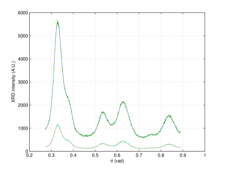
Figure 1: Synthetic XRD intensity profiles as a function of the scattering angle. Table 1 summarizes the parameters used in eq. (10) to compute the diffraction intensities. They are characteristics of Au samples. The wavelength and bulk lattice constant have been set to $\lambda=0.15418$ nm and $a_{f.c.c.}=0.40786$ nm, respectively. From the upper to the lower profile, the NSR increases from $2$ to $5\%$ (see fig. 2 and text for details).

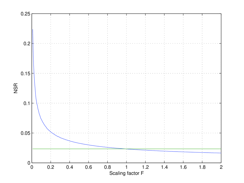
Figure 2: NSR as a function of the factor $F$. See text for details.

where $\mathcal{P}(I)$ denotes a Poisson process with mean value $I$. Figure 1 displays XRD intensity profiles with increasing NSRs. They were obtained by setting $\lambda=0.15418$ nm and $a_{f.c.c.}=0.40786$ nm in eq. (10). The set of parameters used to compute the synthetic profiles are summarized in Table 1. Different NSR values were obtained by scaling the scattered intensity (11) by a factor $F$. Figure 2 shows the NSR of the synthetic profiles as a function of the scaling factor F ranging from 0 to 2. This range contains the NSR values usually measured in experimental profiles

We also considered real data in order to validate our method. Three different samples were prepared with a resultant mean diameter of 2.0, 3.2 and 4.1 nm, respectively (as measured by TEM). The size distributions were approximately characterized by the same width (FWHM $\approx$ 1 nm) for all three systems. Powder XRD studies were realized on the XRD beam line at the Brazilian Synchrotron Light facility (LNLS–Campinas, Brazil) using 8.040 keV photons at room temperature. For further details see Ref. [14].

4 Numerical results

Noisy synthetic XRD patterns were generated corresponding to nanocrystalline samples of increasing size from 2 to 4 nm, and Poisson-distributed noise with increasing NSR from 2% to 10%. The HLSVD–PRO filter was then applied to the noisy synthetic XRD signals in order to study its properties under controlled conditions. A key step in the filtering procedure is the selection of the number $K$ of damped sinusoids characterizing the model function of the HLSVD–PRO filter. Here, a possible approach is presented, which is based on the following frequency selection criterion: the singular values $\lambda_{k}$, $k=1,\dots,r$, are plotted vs. the corresponding frequencies $f_{k}$ of the sinusoids in eq. (1). This choice facilitates a direct comparison of the results of the proposed filter with those obtained by other filters based on a frequency approach. It was observed that, generally, crystallographic XRD intensity signals show a clear transition from a low-frequency region, characterized by high singular values $\lambda_{k},$ to a high-frequency region with small singular values. The index $K$ of the frequency $f_{K}$ corresponding to the transition, provides the number of damped sinusoids to be used in the HLSVD–PRO filter.

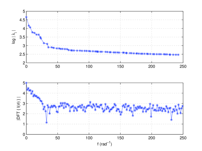
Figure 4: 3 nm Au synthetic sample with NSR = $10\%$: (top) amplitude of eigenvalues $\lambda_{k}$ vs. frequency $f_{k}$, $k=1,\dots,r$. The frequency $f_{K}=35$ rad^-1 was used to separate (filter) high frequency components due to noise; (bottom) Portion of the DFT amplitude spectrum of the noisy synthetic XRD intensity profile. Both plots refer to the XRD intensity profile shown at the top of fig. (3).

Figure 3 displays an example of application of the HLSVD–PRO filter. A noisy synthetic XRD intensity profile is shown at the top of the figure. It corresponds to X-ray scattering from a Au sample having a 3 nm size with a Poisson-like noise with NSR=10%. The filtered signal shown in the middle of the figure was obtained by setting $K=9$ in the HLSVD–PRO filter. This value was estimated by visually inspecting the plot of the singular values $\lambda_{k}$ vs the frequencies $f_{k}$ (see top of fig. (4)). Specifically, a transition from high to small $\lambda_{k}$ was observed at frequency $f_{K}=35$ rad${}^{-1},$ which represents the $K^{th}$ frequency in the set of the sorted frequencies starting from the smallest one. For a comparison, the discrete Fourier transform (DFT) of the noisy synthetic XRD signal is reported at the bottom of fig. (4). Again, a phenomenon of transition from high to small singular values occurs in the same region of the spectrum, as observed at the top of figure. However, the transition frequency is much more difficult to localize than in the HLSVD–PRO filter case. This makes troublesome the application of DFT and WF filters to clean noisy XRD data. It is worth noting that this difference between the HLSVD–PRO and Fourier frequency based filters is relevant when the filter is intended to be used during interactive XRD data analysis. In this case the successful application of a blackbox filter easy-to-use becomes crucial.

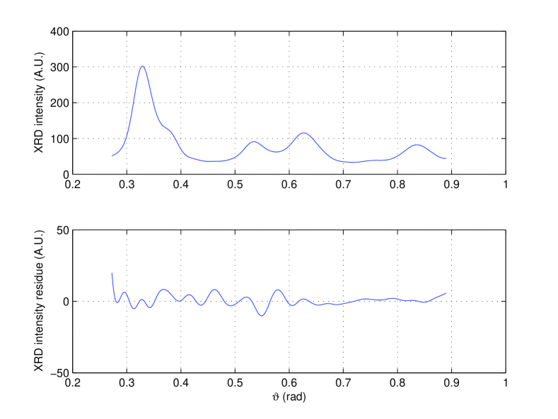
Figure 5: 3 nm Au synthetic sample with NSR = $10\%$: (top) noiseless synthetic XRD intensity profile as a function of the scattering angle $\vartheta$; (bottom) difference between noiseless and filtered (see middle plot of fig. (3)) profiles.

Coming back to fig. (3), the difference between the values of noisy and filtered profiles is shown at the bottom. To quantify the performance of the filter, the filtered signal was compared with the noiseless synthetic XRD signal (see fig. (5)). This can be done only with synthetic signals as experimental XRD data without noise are not available. The filter performance was evaluated using the measure

$${\mathcal{E}}=\frac{||I_{exp}-I_{th}||}{||I_{fil}-I_{th}||}\;,$$ (13)

To give a statistical significance to these measures a Monte Carlo experiment was carried out. More precisely, the HLSVD–PRO was applied to 1000 noisy synthetic profiles generated by starting from the same sample size, with different NSRs. For each filtered profile, the measure ${\mathcal{E}}$ of filter performance was estimated by calculating the mean value and the standard deviation. Table 2 summarizes the outcome of the aforementioned Monte Carlo experiments. For each sample size and NSR, the mean and standard deviation are obtained using $1000$ synthetic XRD intensity profiles with different noise realizations having the same NSR. The sensitivity to the number $K$ of sinusoids of the HLSVD–PRO filter was also studied. This number was slightly varied around the optimal $K$ value selected by using the frequency criterion. The performance results were compared in order to validate the choice of the optimal $K$ value. In particular, $K$ was increased and decreased by 2, as discussed in Section I. The results of such a comparison are summarized in Table 3 and show that the proposed frequency criterion provides the value of $K$ corresponding to the best performance of the HLSVD–PRO filter. The filter was also applied to real XRD intensity profiles of Au samples of size 2, 3.2 and 4.1 nm. Figure 6 shows at top the profile of a 3.2 nm Au sample with $NSR=2.3\%$ computed as $||\sigma||/||I||$, where $\sigma$ and $I$ are vectors with the measured error and the intensity values, respectively. Since in the case of XRD signals the noise follows the Poisson distribution, $\sigma$ is given by $\sqrt{I}$. The result obtained by HLSVD–PRO is displayed in the middle of the figure. At bottom the plot of singular values is depicted vs. the frequency. Components with a frequency higher than $f_{K}=34$ rad^-1, due to noise, were removed. Denoising a real XRD profile of 500 intensity data samples, as typical ones used in the present study, requires about 11 seconds, using MatLab 7 on a machine with a Intel Xeon 1.80 GHz processor and a 512 KB cache size.

5 Conclusions

A filter based on the HLSVD–PRO method has been presented. It has been applied to filter XRD patterns of nanocluster powders. The filter performance has been studied on synthetic and real XRD patterns with different NSRs. Results show that the proposed filter is robust and computationally efficient. A further advantage is its user-friendliness that makes it a useful blackbox tool for the processing of XRD data.

6 Acknowledgments

We thank A. Cervellino, C. Giannini and A. Guagliardi for kindly providing us with experimental XRD data.

Table 1: Values of parameters used in eq. (10) to compute synthetic XRD intensity profiles. The wavelength and the $f.c.c.$ bulk lattice constant were set to $\lambda=0.15418$ nm and $a_{f.c.c.}=0.40786$ nm, respectively.

Parameter	${\mathcal{X}}={\mathcal{C}}$	${\mathcal{X}}={\mathcal{I}}$	${\mathcal{X}}={\mathcal{D}}$
$\xi_{\mathcal{X}}$	5.0	5.0	5.0
$s_{\mathcal{X}}$	0.3	0.3	0.3
$n^{0}_{\mathcal{X}}$	4.0	4.0	6.0
$\Omega_{\mathcal{X}}$	1.0	1.0	1.0
$\Xi_{\mathcal{X}}$	1.0	1.0	1.0
$w_{\mathcal{X}}$	0.5	0.5	0.5

Table 2: Measure ${\mathcal{E}}$ of the filter performance (see eq. 13). For each sample size and NSR, mean and standard deviation figures refer to Monte Carlo experiments run on $1000$ synthetic XRD intensity profile with different noise realizations having the same NSR.

	NSR=2%	NSR=5%	NSR=10%
2 nm	$1.89\pm 0.28$	$2.34\pm 0.18$	$2.49\pm 0.16$
3 nm	$1.54\pm 0.39$	$1.87\pm 0.16$	$2.34\pm 0.20$
4 nm	$1.25\pm 0.06$	$1.56\pm 0.12$	$1.89\pm 0.19$

Table 3: Measure ${\mathcal{E}}$ (see eq. 13) of the filter performance as a function of the order $K$ of the filter, namely the cutoff frequency $f_{K}$. The synthetic XRD intensity data refer to different sample sizes and NSRs.The best performance corresponds to the order $K$ reported in the middle row of each NSR value.

		2 nm	3 nm	4 nm
	K-2	$1.86\pm 0.16$	$1.25\pm 0.09$	$1.67\pm 0.10$
NSR=10%	K=9	$2.49\pm 0.16$	$2.34\pm 0.20$	$1.89\pm 0.19$
	K+2	$2.43\pm 0.42$	$2.28\pm 0.21$	$1.73\pm 0.18$
	K-2	$2.17\pm 0.18$	$1.81\pm 0.16$	$1.52\pm 0.11$
NSR=5%	K=11	$2.34\pm 0.18$	$1.87\pm 0.16$	$1.56\pm 0.12$
	K+2	$2.22\pm 0.28$	$1.87\pm 0.16$	$1.48\pm 0.09$
	K-2	$1.80\pm 0.21$	$1.37\pm 0.32$	$1.13\pm 0.14$
NSR=2%	K=15	$1.89\pm 0.28$	$1.54\pm 0.39$	$1.25\pm 0.06$
	K+2	$1.86\pm 0.18$	$1.46\pm 0.38$	$1.18\pm 0.09$

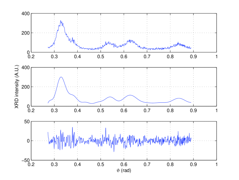
Figure 3: 3 nm Au synthetic sample: (top) noisy (NSR=$10\%$) synthetic XRD intensity profile as a function of the scattering angle $\vartheta$; (middle) filtered XRD intensity profile. The HLSVD–PRO filter removes signal components with frequency above $f_{K}=35$ rad^-1 (see fig. (4)); (bottom) difference between measured and filtered profiles.

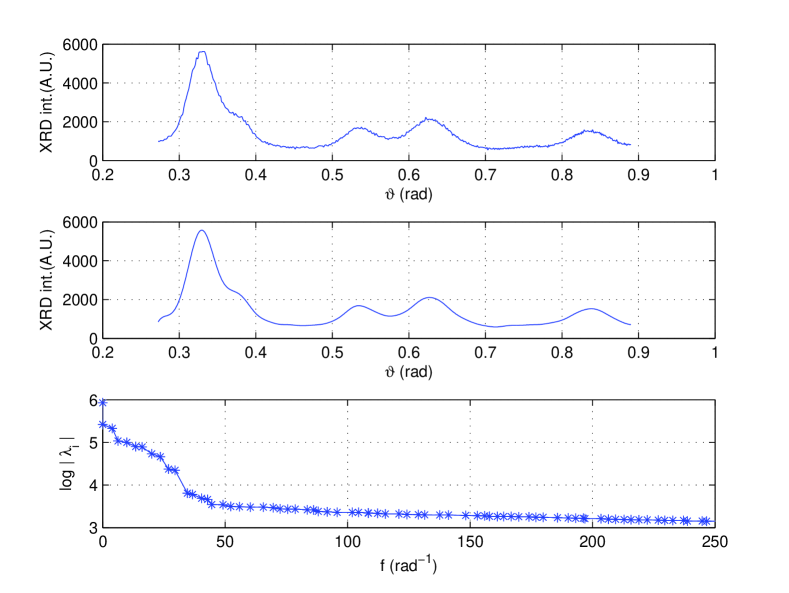
Figure 6: 3.2 nm Au real sample: (top) noisy (NSR=2.3%) XRD intensity profile as a function of the scattering angle $\vartheta$; (middle) filtered XRD intensity profile. The HLSVD–PRO filter removes signal components with frequency above $f_{K}=34$ rad^-1; (bottom) amplitudes of eigenvalues $\lambda_{k}$ vs frequency $f_{k}$, $k=1,...,q$.

References

- [1] B. Mierzwa, J. Pielaszek, Smoothing of low-intensity noisy X-ray diffraction data by Fourier filtering: application to supported metal catalyst studies, Journal of Applied Crystallography, 30, 544-546, 1997.
- [2] A. Hieke, H.D. Dörfler, Methodical developments for X-ray diffraction measurements and data analysis on lytropic liquid crystals applied to K-soap/glyceral systems, Colloid Polym. Sci., 277, 762-776, 1999.
- [3] M. Schmidt, S. Rajagopal, Z. Ren, K. Moffat, Application of Singular Value Decomposition to the analysis of time-resolved macromolecular X-ray data, Biophysical Journal, 84, 2112-2129, 2002.
- [4] S. Rajagopal, M.Schmidt, S. Anderson, H. Ihee, K. Moffat, Analysis of time-resolved crystallographic data by singular value decomposition, Acta Crystallographica, D60, 860-871, 2004.
- [5] E.E. Aubanel, K.B. Oldham, Fourier smoothing without the fast fourier transform, Byte, 10(2), 207-222, 1985.
- [6] C. Wooff, Smoothing of data by least squares fitting, Comput. Phys. Commun., 42, 249-251, 1986.
- [7] H. Barkhuijsen, R. De Beer, D. Van Ormondt, Improved algorithm for noniterative time-domain model fitting to exponentially damped magnetic resonance signals, Journal of Magnetic Resonance, 73, 553-557, 1987.
- [8] T. Laudadio, N. Mastronardi, L. Vanhamme, P. Van Hecke and S. Van Huffel, Improved Lanczos Algorithms for Blackbox MRS Data Quantitation, Journal of Magnetic Resonance, 157, 292-297, 2002.
- [9] D.J. Wales, Structure, dynamics, and thermodynamics of clusters: tales from topographic potential surfaces, Science, 271, 925-929, 1996.
- [10] R.W. Siegel, E. Hu, D.M. Cox, H. Goronkin, L. Jelinski, C.C. Koch, J. Mendel, M.C. Roco, D.T. Shaw, Nanostructure Science and Technolgy. A Worldwide Study, The Interagency Working Group on NanoScience, Engineering and Technolgy, http://itri.loyola.edu/nano.
- [11] H. D. Simon, The Lanczos algorithm with partial reorthogonalization, Math. Comp., 42, 115-142, 1984.
- [12] R.A. Young, The Rietvel method, 417-420, Oxford University Press, 1993.
- [13] A. Cervellino, C. Giannini and A. Guagliardi, Determination of nanoparticle structure type, size and strain distribution from X-ray data for monoatomic f.c.c.-derived non-crystallographic nanoclusters, Journal of Applied Crystallography, 36, 1148-1158, 2003.
- [14] D. Zanchet, B.D. Hall and D. Ugarte, Structure population in thiol-passivated nanoparticles, Journal of Physical Chemistry, 104, 11013-11018, 2000.