A new construction of perfectly matched layers for the linearized Euler equations
Abstract
Based on a PML for the advective wave equation, we propose two PML models for the linearized Euler equations. The derivation of the first model can be applied to other physical models. The second model was implemented. Numerical results are shown.
1 Introduction
Since the work by Berenger on perfectly matched layer for the Maxwell equations [Ber94, Ber96] in a computational box, many works have been devoted to a better understanding of their principle and behaviour see [MPV98], [ZC96], [CW94], [LS00] [MC98] [BFJ03][BJ02] [AGH02] to extensions to other geometries, see [ST04] [CM98], or equations see [HN02] [AGH99][DJ03] . We consider here the linearized Euler equations which has been the subject of many works, see [Rah04], [Hu01], [TAC98] [Hes98] [Hu96] [Hag03] (and references therein). The key issue is a possible lack of long time stability [Hes98, TAC98]. A first stable PML was proposed in [Hu01] for flows normal to the boundary. It has been recently extended to oblique flows in [Hag03], see also [FDFT02]. In these works, the PML is obtained via a change of coordinate in the complex plane applied to the direction normal to the boundary (say ). This amounts to replacing all the derivatives in the Euler system by an operator denoted by which is still differential in the direction but pseudo-differential in the other variables. Based on the Smith factorization [WRL95], we propose here another strategy for constructing stable PMLs. The main feature is that not all derivatives are modified. The Euler system is modified only in order to damp the modes that could reflect at the interface between the physical domain and the PML. In our approach, the vorticity modes which are convected by a transport operator are not damped since they leave naturally the computational domain at an outflow boundary. As a result, even after discretization, the vorticity in the PML region equals (up to the machine accuracy) the vorticity of the reference solution computed in a very large domain, see figure 3 in § 4.
Moreover, the technique introduced in this paper enables an appropriate “PML” treatment of the various scalar equations at the basis of the system of PDEs under consideration. We think therefore that the technique introduced in this paper should extend to other systems of PDEs as well (e.g. shallow water, anistropic elasticity, ).
More precisely, in section 2 we introduce the Smith factorization of the Euler equation. This powerful tool is used in section 3 to propose two ways to design PML for the Euler equation (see [DNR05] for the application of the Smith factorization in domain decomposition methods). Both PMLs are based on the use of a PML for the underlying advective wave equation. The derivation of the first model can be applied to other physical models. In section 4, numerical results are shown for the second model which is easier to implement.
2 Analysis of the Euler system via Smith factorization
We write the linearized Euler equations around a constant subsonic flow , a constant density and a constant speed of sound as:
| (1) |
where is a given right handside.
2.1 Smith factorization
We first recall the definition of the Smith factorization of a matrix with polynomial entries and apply it to systems of PDEs, see [Gan66, Gan98] (or [WRL95] for the mathematical analysis of systems of PDEs) and references therein.
Theorem 2.1
Let be an integer and an invertible matrix with polynomial entries in one variable : .
Then, there exist three matrices with polynomial entries , and with the following properties:
-
•
det() and det() are real numbers.
-
•
is a diagonal matrix.
-
•
.
Morevoer, is uniquely defined up to a reordering and multiplication of each entry by a constant by a formula defined as follows. Let ,
-
•
is the set of all the submatrices of order extracted from .
-
•
-
•
is a largest common divisor of the set of polynomials .
Then,
| (2) |
(by convention, ).
Application to the Euler system
We first take formally the Fourier transform of the system (1) with respect to and (dual variables are and resp.). We keep the partial derivatives in since in the sequel we shall design a PML for a truncation of the domain in the direction. We note
| (3) |
We can perform a Smith factorization of by considering it as a matrix with polynomials in entries. We have
| (4) |
where
| (5) |
and
and
where
| (6) |
and
| (7) |
The operators showing up in the diagonal matrix have a physical meaning:
is a first order transport operator and
is the advective wave operator.
2.2 Modes via Smith factorization
In the PML analysis of section 3, we shall use the expression of solutions to the homogeneous Euler equation. In order to illustrate the previous section, we make use of the Smith factorization to compute them. We take the Fourier transform in and of (1) and seek non zero solutions to
Using Smith factorization (4), we have
Since det is a real number, is still a matrix with polynomials in entries so that we can apply it to the above equation and get:
This implies that
| (8) |
where . Since is of third order in the direction, we have three possible values for :
| (9) |
| (10) |
| (11) |
Remark 1
comes from the transport operator whereas come from the advective wave operator .
Since det is a real number, is still a matrix with polynomials in entries so that we can apply it to equation (8) and get:
| (12) |
We shall define, for
| (13) |
It is easy to check that indeed does not depend on and that
| (14) |
In the classical mode analysis of a system of PDEs, vectors are obtained after the diagonalization of a matrix. Using the Smith factorization simplifies the computation since these vectors are given by the explicit formula (13) and not by an eigenvalue computation.
Notation Let and be integers. For a matrix , denotes the entry of the -th row and of the -th column. For a vector , denotes its -th component.
Remark 2
In section 3.5, we shall use that
| (15) |
3 PMLs for the Euler System
The Smith factorization of the Euler system (4) and the computations of the previous section show that the modes correspond either to operator or to operator . Among these two operators, the only operator which generates waves propagating in both positive and negative directions is the operator . This suggests that designing a PML for the Euler equation can be reduced to the design of PML for the advective wave operator .
3.1 PML for the advective wave equation
This question has been the subject of several works, [Hag03], [FDFT02], [HN02], [BBBDL04] [DJ03] [BBBDL03] and references therein. Following these works, we use the for operator a PML defined by replacing the derivatives by a “pml” derivative. The definition is as follows. Let be the damping parameter of the PML and is the inverse Fourier transform in the variables and , we define the pseudo-differential operator :
| (16) |
We define the derivative by
| (17) |
We are now in position to define the PML- equations of the advective wave operator :
| (18) |
Let us notice that we have
| (19) |
where the operator is a pseudo-differential operator in the and variables:
| (20) |
A PML- used for truncating the domain in the direction would consist in replacing in the operator the derivatives by a “pml” derivative in the direction defined as follows:
| (21) |
The PML- equations of the advective wave operator for the truncation of the domain in the direction read:
| (22) |
In order to give a complete definition of a PML bordering a rectangular computational domain, we have three possibilities for the corner region.The first one consists in desiging a third PML model in the corner that is compatible with both PML- and PML- as was done for the Maxwell system in [Ber94] for instance. The second possibility is to use prismatoidal coordinates [LS01]. The advantage is that it allows for arbitrary convex computational domains and not only rectangular ones. The third possibility consists simply in placing side by side PML- and PML- regions. We have implemented this last simple approach and obtain good results, see § 4. Of course, the two first options deserve further investigations.
3.2 First PML model
Based on (4), a first possibility is to define a PML for the Euler system by substitution of with in matrix (see formula (5)). In matrices and and in the operator , the derivatives are not modified. We modify only the advective wave operator. Let
| (23) |
we define a PML for the Euler system
| (24) |
with the following interface conditions between the Euler media and the PML
| (25) |
where the subscript 3 denotes the third component of a vector.
Study of the first PML media
We now give the results of an analysis of the PML system similar to that of § 2.2 for the Euler system. We define
and for
| (26) |
It is easy to check that indeed does not depend on and that for any solution to the homogeneous first PML system there exist such that
| (27) |
If we consider the solution in the positive half space, its boundedness as tends to infinity implies that .
3.3 PMLness of the first model
A key property of a PML is that there is no reflection at the interface between the Euler media and the PML media. We will prove that it is the case for a truncation of the space with an infinite PML starting at with a independant damping parameter . We have to consider the following coupled problem:
Find such that:
| (28) |
with the interface conditions (25)
| (29) |
We take the Fourier transform in and of (28) and get:
| (30) |
From section 2.2, we know that the general solution to the Euler system is :
| (31) |
where is defined in (13). As for the solution in the PML media, we know from (27) and the boundedness of the solution as tends to infinity that
| (32) |
We study the adequacy of the PML by considering and to be given. This corresponds to ingoing waves from the Euler media and moving towards the interface between the Euler media and the PML media. The three other quantities ( are determined by the interface conditions (29). The media is perfectly matched if we have no reflection in the Euler media, i.e. if . We now prove that this is indeed the case.
From (31) and (13), we have:
| (33) |
| (34) |
Let
Notice that
and that
so that the interface conditions (29) yield:
| (35) |
Thus we have
The nullity of shows that there is no reflection at the interface between the Euler and an infinite PML media.
In practice, the PML has a finite width. As a result, the coefficient will not be zero in general. But, the corresponding mode is exponentially decreasing as is increasing. Its contribution to the solution on the interface can be made as small as necessary simply by increasing the width of the PML.
Complexity of the first PML model
A direct computation yields:
| (36) |
where
The difference with the Euler system concerns only the last equation on the variable , but :
-
1.
The formula is complex and involves third order derivatives on both the pressure and the normal velocity .
-
2.
The formula implies a division by which can be zero.
As for the first point, one might argue that it is just a matter of implementation. The second point seems more serious. A possible cure could be to take:
where . From formulas for and and formula (19)-(20), we get then
As a result the symbols of and would not vanish. But it would be at the expense of the damping of the PML. Indeed, would be small for small values of or of . The present first model raises difficulties. Nevertheless, it should deserve interest since it corresponds to a systematic way to design a PML for systems of PDEs. Moreover, since matrices and are not unique, it is quite possible that a more suitable Smith factorization when used in formula (24) would lead to a practicable PML. In the next section, we design another PML for the Euler system whose numerical results will be given in section 4.
3.4 Second PML model
The rationale for this model is that the pressure satisfies an advective wave equation which is the only equation that demands a PML. Indeed, let multiply (3) by the matrix
| (37) |
We get:
| (38) |
We substitute with and apply
and we are thus led to define:
| (39) |
A direct computation yields:
| (40) |
In order to get rid of the operator , we introduce a new variable such that so that in the physical space the enlarged PML system we consider reads:
| (41) |
with the following interface conditions between the Euler media and the PML
Study of the second PML media
We now proceed to an analysis of the PML system similar to that of § 2.2 for the Euler system. The Smith factorization of reads
where
| (42) |
and and are matrices with polynomial in entries and their determinants are one. This will enable us to give the general form of the solutions to the homogeneous PML equations. Indeed, let us denote such a solution. From the Smith factorization, there exist such that
where
By applying to the above equation, we see that there exist vectors , such that
| (43) |
If we consider the solution in the positive half space, its boundedness as tends to infinity implies that .
3.5 PMLness of the second model
We proceed similarly to § 3.3. We will prove there is no reflection at the interface between the Euler media and the PML media for a truncation of the space with an infinite PML starting at with a constant damping parameter . We consider the following coupled problem:
Find such that:
| (44) |
We take the Fourier transform in and of the above coupled system and get:
| (45) |
From section 2.2, we know that the general solution to the Euler system is :
where is defined in (13). As for the solution in the PML media, we know from (43) and the boundedness of the solution as tends to infinity that
We study the adequacy of the PML by considering and to be given. This corresponds to ingoing waves from the Euler media and moving towards the interface between the Euler media and the PML media. The four other quantities ( are determined by the interface conditions. The media is perfectly matched if we have no reflection in the Euler media, i.e. if . We now prove that this is indeed the case. We focuse on the equation satisfied by the pressure. By applying matrix
to , we have that satisfies the equation of advective Helmholtz PML media:
From (38), we also have that
The interface conditions on the pressure are and . We know from works on PML for the convective Helmholtz that there is no reflection at the interface for the pressure. Therefore there exists such that
| (46) |
We prove now that as a consequence, is zero. Indeed, taking the first component of (43) we have that
| (47) |
So that we have whereas for . Thus we can infer from (46) and (47) that . This shows that there is no reflection at the interface between the Euler and an infinite PML media.
In practice, the PML has a finite width. As a result, the coefficient will not be zero in general. But, the corresponding mode is exponentially decreasing as is increasing. Its contribution to the solution on the interface can be made as small as necessary simply by increasing the width of the PML.
Remark 3 (PMLs for the 3D Euler system)
Using obvious notations, we briefly mention that the design of a PML for the three-dimensional Euler system:
| (48) |
is very similar to the two-dimensional case. Let be the 3D first order transport operator and the 3D acoustic wave equation. The Smith form of the 3D compressible Euler equations is
As in the 2D case, only the advective wave operator needs a “pml” procedure. For instance, the second model should read:
4 Numerical Results
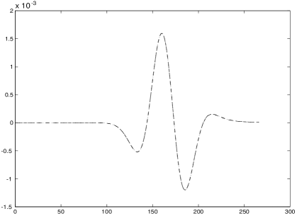
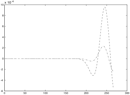
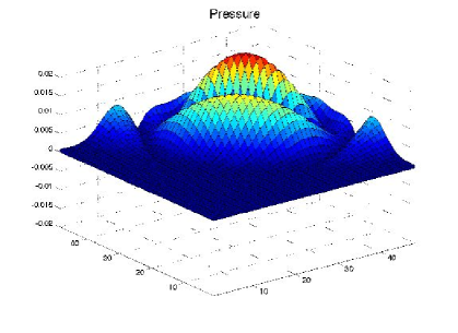
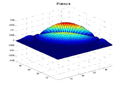
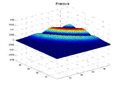
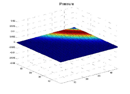
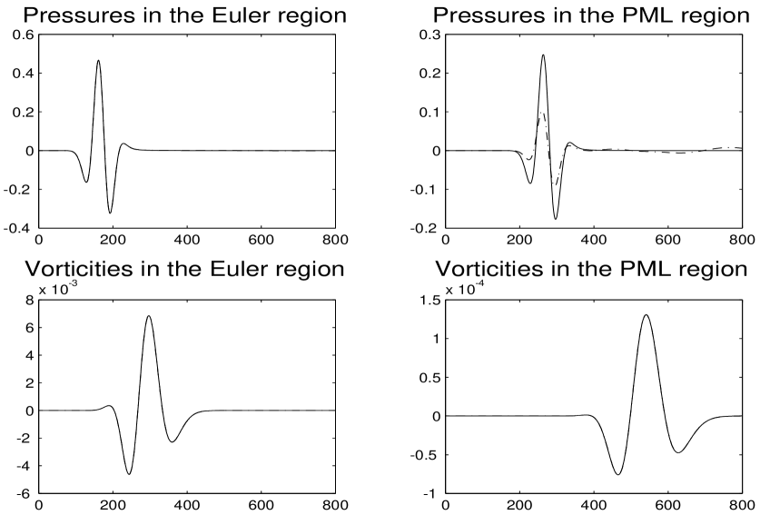
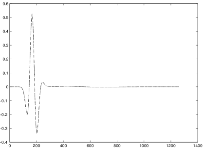
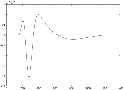
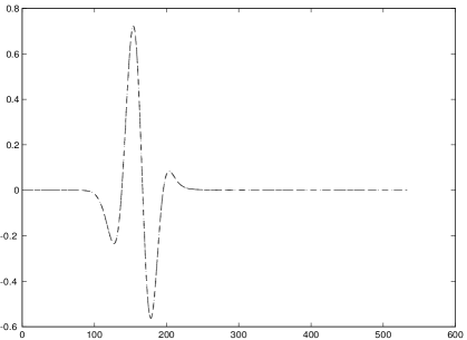
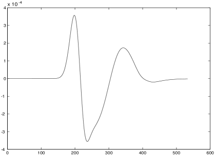
We have taken and . The 2D linearized Euler equations are discretized on a uniform staggered grid using a Yee Scheme and a CFL equals to . The convective derivatives are discretized using an upwind scheme both in the Euler region and in the PMLs. The computational domain is the square and except in table 1, PMLs have a width corresponding to grid points. The damping parameter depends on the coordinate normal to the interface (say ): where is a positive constant. The initial solutions are zero. Let for and zero for with , and is the Dirac mass located in the middle of the computational domain. The right handside was on all three equations of system (1) except for figure 1 where it was zero on the velocity components. The PML solution is compared with a reference solution that is computed on a much larger domain. In figure 1, the pressure for both solutions are plotted as a function of time 4 points from the upperleft corner of the domain (left figure) and inside the PML (right figure). The velocity field is . In the Euler region, both curves are nearly identical. In the PML, we see the damping of the PML solution. Of course, for the reference solution, this corresponds to an Euler region and there is no damping. In Figure 3 we have the same plot for the pressure and the vorticity as well, in this case and . In agreement with the construction of the PML, we see that the vorticity is not damped at all in the PML region. The vorticity in the PML region equals that of the reference solution. Indeed, in the construction of the PML in (38) only the wave operator is “pml”-ized and the transport operator is not modified. In figure 2, we show the pressure at different times of the computation for an oblique velocity . For the same computation, pressure near the upperleft corner is shown on Figure 4. Figure 5 is a similar figure for a horizontal flow in a duct.
In table 1, we study the influence of the parameters of the PML on the error between the reference solution and the pml solution. We see that with a generous PML ( grid points), the error is indeed very small. With grid points, the error is small and with points results are not satisfactory even when using various parameters . It is worth noticing that due to the use of an upwind scheme for the transport operator, the error on the vorticity is equal to the machine accuracy for any layer parameters.
| Relative error in percentage vs. (, ) | ||||||
| variable | (, ) | (, ) | (, ) | (, ) | (, ) | (, ) |
| 0.12 | 1.0 | 8.0 | 10.0 | 6.0 | 1.0 | |
| 0.25 | 1.2 | 0.4 | 16.3 | 0.4 | 0.3 | |
| 0.1 | 0.1 | 10.0 | 20.8 | 0.4 | 10.0 | |
The long time stability of the PML was assessed by computing on time intervals five times longer than those used for generating the figures. No instability was observed for various flows.
5 Conclusion
The first PML model proposed in § 3.2 is obtained by using the Smith factorization of the Euler equations and a PML for the advective wave equation. This method can be applied to other systems of partial differential equations (free-surface flow, anisotropic elasticity, ). The second PML model we have proposed for the Euler linearized equations are based on the PML for the advective wave equation. Thus, the PML for Euler inherits the properties from the latter. This second model was implemented and numerical results illustrate the efficiency of the approach.
References
- [AGH99] S. Abarbanel, D. Gottlieb, and J. S. Hesthaven. Well-posed perfectly matched layers for advective acoustics. J. Comput. Phys., 154(2):266–283, 1999.
- [AGH02] S. Abarbanel, D. Gottlieb, and J. S. Hesthaven. Long time behavior of the perfectly matched layer equations in computational electromagnetics. In Proceedings of the Fifth International Conference on Spectral and High Order Methods (ICOSAHOM-01) (Uppsala), volume 17, pages 405–422, 2002.
- [BBBDL03] Eliane Bécache, Anne-Sophie Bonnet-Ben Dhia, and Guillaume Legendre. Perfectly matched layers for the convected Helmholtz equation. In Mathematical and numerical aspects of wave propagation—WAVES 2003, pages 142–147. Springer, Berlin, 2003.
- [BBBDL04] E. Bécache, A.-S. Bonnet-Ben Dhia, and G. Legendre. Perfectly matched layers for the convected Helmholtz equation. SIAM J. Numer. Anal., 42(1):409–433 (electronic), 2004.
- [Ber94] J.P. Berenger. A perfectly matched layer for the absorption of electromagnetic waves. J. Comput. Phys., 114(2):185–200, 1994.
- [Ber96] J. P. Berenger. Three-dimensional perfectly matched layer for the absorption of electromagnetic waves. J. Comput. Phys., 127(2):363–379, 1996.
- [BFJ03] E. Bécache, S. Fauqueux, and P. Joly. Stability of perfectly matched layers, group velocities and anisotropic waves. J. Comput. Phys., 188(2):399–433, 2003.
- [BJ02] Eliane Bécache and Patrick Joly. On the analysis of Bérenger’s perfectly matched layers for Maxwell’s equations. M2AN Math. Model. Numer. Anal., 36(1):87–119, 2002.
- [CM98] Francis Collino and Peter Monk. The perfectly matched layer in curvilinear coordinates. SIAM J. Sci. Comput., 19(6):2061–2090 (electronic), 1998.
- [CW94] W. C. Chew and W. H. Weedon. A 3d perfectly matched medium from modified maxwell’s equations with stretched coordinates. IEEE Trans. Microwave Opt. Technol. Lett., 7:599–604, 1994.
- [DJ03] Julien Diaz and Patrick Joly. Stabilized perfectly matched layer for advective acoustics. In Mathematical and numerical aspects of wave propagation—WAVES 2003, pages 115–119. Springer, Berlin, 2003.
- [DNR05] V. Dolean, F. Nataf, and G. Rapin. New constructions of domain decomposition methods for systems of pdes. Comptes Rendus Académie des Sciences, Série I, 2005.
- [FDFT02] Dubois F., E. Duceau, Maréchal F., and I. Terrasse. Lorentz transform and straggered finite differences for advective acoustics. Technical report, EADS, 2002.
- [Gan66] F. R. Gantmacher. Théorie des matrices. Tome 1: Théorie générale. Traduit du Russe par Ch. Sarthou. Collection Universitaire de Mathématiques, No. 18. Dunod, Paris, 1966.
- [Gan98] F. R. Gantmacher. The theory of matrices. Vol. 1. AMS Chelsea Publishing, Providence, RI, 1998. Translated from the Russian by K. A. Hirsch, Reprint of the 1959 translation.
- [Hag03] Th. Hagstrom. A new construction of perfectly matched layers for hyperbolic systems with applications to the linearized Euler equations. In Math. and num. aspects of wave propagation—WAVES 2003, pages 125–129. Springer, 2003.
- [Hes98] J. S. Hesthaven. On the analysis and construction of perfectly matched layers for the linearized Euler equations. J. Comput. Phys., 142(1):129–147, 1998.
- [HN02] T. Hagstrom and I. Nazarov. Absorbing layers and radiation boundary conditions for jet flow simulations. In Proc. of the 8th AIAA/CEAS aeroacoustics conference, volume 60, 2002.
- [Hu96] Fang Q. Hu. On absorbing boundary conditions for linearized Euler equations by a perfectly matched layer. J. Comput. Phys., 129(1):201–219, 1996.
- [Hu01] Fang Q. Hu. A stable, perfectly matched layer for linearized Euler equations in unsplit physical variables. J. Comput. Phys., 173(2):455–480, 2001.
- [LS00] M. Lassas and E. Somersalo. On the existence and convergence of the solution of pml equations. Computing, 60:229–241, 2000.
- [LS01] Matti Lassas and Erkki Somersalo. Analysis of the PML equations in general convex geometry. Proc. Roy. Soc. Edinburgh Sect. A, 131(5):1183–1207, 2001.
- [MC98] P. Monk and F. Collino. Optimizing the perfectly matched layer. In IUTAM Symposium on Computational Methods for Unbounded Domains (Boulder, CO, 1997), volume 49 of Fluid Mech. Appl., pages 245–254. Kluwer Acad. Publ., Dordrecht, 1998.
- [MPV98] R. Mittra, Ü. Pekel, and J. Veihl. A theoretical and numerical study of Berenger’s perfectly matched layer (PML) concept for mesh truncation in time and frequency domains. In Approximations and numerical methods for the solution of Maxwell’s equations (Oxford, 1995), volume 65 of Inst. Math. Appl. Conf. Ser. New Ser., pages 1–19. Oxford Univ. Press, New York, 1998.
- [Rah04] Adib N. Rahmouni. An algebraic method to develop well-posed PML models. Absorbing layers, perfectly matched layers, linearized Euler equations. J. Comput. Phys., 197(1):99–115, 2004.
- [ST04] I. Singer and E. Turkel. A perfectly matched layer for the Helmholtz equation in a semi-infinite strip. J. Comput. Phys., 201(2):439–465, 2004.
- [TAC98] Christopher K. W. Tam, Laurent Auriault, and Francesco Cambuli. Perfectly matched layer as an absorbing boundary condition for the linearized Euler equations in open and ducted domains. J. Comput. Phys., 144(1):213–234, 1998.
- [WRL95] J. T. Wloka, B. Rowley, and B. Lawruk. Boundary value problems for elliptic systems. CUP, Cambridge, 1995.
- [ZC96] L. Zhao and A. C. Cangellaris. GT-PML: Generalized theory of perfectly matched layers and its application to the reflectionless truncation of finite-difference time-domain grids. IEEE Trans. Microwave Theory Tech, 44:2555–2563, 1996.