Global Conservative Solutions to a Nonlinear Variational Wave Equation

Abstract

We establish the existence of a conservative weak solution to the Cauchy problem for the nonlinear variational wave equation $u_{tt}-c(u)(c(u)u_{x})_{x}=0$, for initial data of finite energy. Here $c(\cdot)$ is any smooth function with uniformly positive bounded values.

Mathematics Subject Classification (2000): 35Q35
Keywords: Existence, uniqueness, singularity, coordinate transformation

1 Introduction

We are interested in the Cauchy problem

$$u_{tt}-c(u)\big{(}c(u)u_{x}\big{)}_{x}=0\,,$$ (1.1)

with initial data

$$u(0,x)=u_{0}(x)\,,\qquad u_{t}(0,x)=u_{1}(x)\,.$$ (1.2)

Throughout the following, we assume that $c:{\mathbb{R}}\mapsto{\mathbb{R}}_{+}$ is a smooth, bounded, uniformly positive function. Even for smooth initial data, it is well known that the solution can lose regularity in finite time ([12]). It is thus of interest to study whether the solution can be extended beyond the time when a singularity appears. This is indeed the main concern of the present paper. In ([5]) we considered the related equation

$$u_{t}+f(u)_{x}={1\over 2}\int_{0}^{x}f^{\prime\prime}(u)u_{x}^{2}\,dx$$ (1.3)

and constructed a semigroup of solutions, depending continuously on the initial data. Here we establish similar results for the nonlinear wave equation (1.1). By introducing new sets of dependent and independent variables, we show that the solution to the Cauchy problem can be obtained as the fixed point of a contractive transformation. Our main result can be stated as follows. Theorem 1. Let $c:{\mathbb{R}}\mapsto[\kappa^{-1},\,\kappa]$ be a smooth function, for some $\kappa>1$. Assume that the initial data $u_{0}$ in (1.2) is absolutely continuous, and that $(u_{0})_{x}\in{\bf L}^{2}\,$,  $u_{1}\in{\bf L}^{2}$. Then the Cauchy problem (1.1)-(1.2) admits a weak solution $u=u(t,x)$, defined for all $(t,x)\in{\mathbb{R}}\times{\mathbb{R}}$. In the $t$-$x$ plane, the function $u$ is locally Hölder continuous with exponent $1/2$. This solution $t\mapsto u(t,\cdot)$ is continuously differentiable as a map with values in ${\bf L}^{p}_{\rm loc}$, for all $1\leq p<2$. Moreover, it is Lipschitz continuous w.r.t. the ${\bf L}^{2}$ distance, i.e.

$$\big{\|}u(t,\cdot)-u(s,\cdot)\big{\|}_{{\bf L}^{2}}\leq L\,|t-s|$$ (1.4)

for all $t,s\in{\mathbb{R}}$. The equation (1.1) is satisfied in integral sense, i.e.

$$\int\!\!\int\Big{[}\phi_{t}\,u_{t}-\big{(}c(u)\phi\big{)}_{x}c(u)\,u_{x}\Big{]}\,dxdt=0$$ (1.5)

for all test functions $\phi\in{\cal C}^{1}_{c}$. Concerning the initial conditions, the first equality in (1.2) is satisfied pointwise, while the second holds in ${\bf L}^{p}_{\rm loc}\,$ for $p\in[1,2[\,$. Our constructive procedure yields solutions which depend continuously on the initial data. Moreover, the “energy”

$${\cal E}(t)\doteq\frac{1}{2}\int\Big{[}u_{t}^{2}(t,x)+c^{2}\big{(}u(t,x)\big{)}\,u_{x}^{2}(t,x)\Big{]}\,dx$$ (1.6)

remains uniformly bounded. More precisely, one has Theorem 2. A family of weak solutions to the Cauchy problem (1.1)-(1.2) can be constructed with the following additional properties. For every $t\in{\mathbb{R}}$ one has

$${\cal E}(t)~{}\leq~{}{\cal E}_{0}~{}\doteq~{}\frac{1}{2}\int\Big{[}u_{1}^{2}(x)+c^{2}\big{(}u_{0}(x)\big{)}(u_{0})_{x}^{2}(x)\Big{]}\,dx\,.$$ (1.7)

Moreover, let a sequence of initial conditions satisfy

$$\big{\|}(u_{0}^{n})_{x}-(u_{0})_{x}\big{\|}_{{\bf L}^{2}}\to 0\,,\qquad\qquad\big{\|}u_{1}^{n}-u_{1}\big{\|}_{{\bf L}^{2}}\to 0\,,$$

and $u^{n}_{0}\to u_{0}$ uniformly on compact sets, as $n\to\infty$. Then one has the convergence of the corresponding solutions $u^{n}\to u$, uniformly on bounded subsets of the $t$-$x$ plane. It appears in (1.7) that the total energy of our solutions may decrease in time. Yet, we emphasize that our solutions are conservative, in the following sense. Theorem 3. There exists a continuous family $\{\mu_{t}\,;~{}~{}t\in{\mathbb{R}}\}$ of positive Radon measures on the real line with the following properties.

(i) At every time $t$, one has $\mu_{t}({\mathbb{R}})={\cal E}_{0}$.

(ii) For each $t$, the absolutely continuous part of $\mu_{t}$ has density $\frac{1}{2}(u_{t}^{2}+c^{2}\,u_{x}^{2})$ w.r.t. the Lebesgue measure.

(iii) For almost every $t\in{\mathbb{R}}$, the singular part of $\mu_{t}$ is concentrated on the set where $c^{\prime}(u)=0$.

In other words, the total energy represented by the measure $\mu$ is conserved in time. Occasionally, some of this energy is concentrated on a set of measure zero. At the times $\tau$ when this happens, $\mu_{\tau}$ has a non-trivial singular part and ${\cal E}(\tau)<{\cal E}_{0}$. The condition (iii) puts some restrictions on the set of such times $\tau$. In particular, if $c^{\prime}(u)\not=0$ for all $u$, then this set has measure zero. The paper is organized as follows. In the next two subsections we briefly discuss the physical motivations for the equation and recall some known results on its solutions. In Section 2 we introduce a new set of independent and dependent variables, and derive some identities valid for smooth solutions. We formulate a set of equations in the new variables which is equivalent to (1.1). Remarkably, in the new variables all singularities disappear: Smooth initial data lead to globally smooth solutions. In Section 3 we use a contractive transformation in a Banach space with a suitable weighted norm to show that there is a unique solution to the set of equations in the new variables, depending continuously on the data $u_{0},u_{1}$. Going back to the original variables $u,t,x$, in Section 4 we establish the Hölder continuity of these solutions $u=u(t,x)$, and show that the integral equation (1.5) is satisfied. Moreover, in Section 5, we study the conservativeness of the solutions, establish the energy inequality and the Lipschitz continuity of the map $t\mapsto u(t,\cdot)$. This already yields a proof of Theorem 2. In Section 6 we study the continuity of the maps $t\mapsto u_{x}(t,\cdot)$, $t\mapsto u_{t}(t,\cdot)$, completing the proof of Theorem 1. The proof of Theorem 3 is given in Section 7.

1.1 Physical background of the equation

Equation (1.1) has several physical origins. In the context of nematic liquid crystals, it comes as follows. The mean orientation of the long molecules in a nematic liquid crystal is described by a director field of unit vectors, ${\mathbf{n}}\in{\mathbb{S}}^{2}$, the unit sphere. Associated with the director field ${\mathbf{n}}$, there is the well-known Oseen-Franck potential energy density $W$ given by

$$W\left({\mathbf{n}},\nabla{\mathbf{n}}\right)=\alpha\left|{\mathbf{n}}\times(\nabla\times{\mathbf{n}})\right|^{2}+\beta(\nabla\cdot{\mathbf{n}})^{2}+\gamma\left({\mathbf{n}}\cdot\nabla\times{\mathbf{n}}\right)^{2}.$$ (1.8)

The positive constants $\alpha$, $\beta$, and $\gamma$ are elastic constants of the liquid crystal. For the special case $\alpha=\beta=\gamma$, the potential energy density reduces to

$$W\left({\mathbf{n}},\nabla{\mathbf{n}}\right)=\alpha\left|\nabla{\mathbf{n}}\right|^{2},$$

which is the potential energy density used in harmonic maps into the sphere ${\mathbb{S}}^{2}$. There are many studies on the constrained elliptic system of equations for ${\mathbf{n}}$ derived through variational principles from the potential (1.8), and on the parabolic flow associated with it, see [3, 9, 10, 16, 22, 36] and references therein. In the regime in which inertia effects dominate viscosity, however, the propagation of the orientation waves in the director field may then be modeled by the least action principle (Saxton [29])

$$\frac{\delta}{\delta u}\int\left\{\partial_{t}{\mathbf{n}}\cdot\partial_{t}{\mathbf{n}}-W\left({\mathbf{n}},\nabla{\mathbf{n}}\right)\right\}\,d{\mathbf{x}}dt=0,\qquad{\mathbf{n}}\cdot{\mathbf{n}}=1.$$ (1.9)

In the special case $\alpha=\beta=\gamma$, this variational principle (1.9) yields the equation for harmonic wave maps from $(1+3)$-dimensional Minkowski space into the two sphere, see [8, 31, 32] for example. For planar deformations depending on a single space variable $x$, the director field has the special form

$${\mathbf{n}}=\cos u(x,t){\mathbf{e}}_{x}+\sin u(x,t){\mathbf{e}}_{y},$$

where the dependent variable $u\in{\mathbb{R}}^{1}$ measures the angle of the director field to the $x$-direction, and ${\mathbf{e}}_{x}$ and ${\mathbf{e}}_{y}$ are the coordinate vectors in the $x$ and $y$ directions, respectively. In this case, the variational principle (1.9) reduces to (1.1) with the wave speed $c$ given specifically by

$$c^{2}(u)=\alpha\cos^{2}u+\beta\sin^{2}u.$$ (1.10)

The equation (1.1) has interesting connections with long waves on a dipole chain in the continuum limit ([13], Zorski and Infeld [45], and Grundland and Infeld [14]), and in classical field theories and general relativity ([13]). We refer the interested reader to the article [13] for these connections.

This equation (1.1) compares interestingly with other well-known equations, e. g.

$$\partial^{2}_{t}u-\partial_{x}[p(\partial_{x}u)]=0,$$ (1.11)

where $p(\cdot)$ is a given function, considered by Lax [25], Klainerman and Majda [24], and Liu [28]. Second related equation is

$$\partial_{t}^{2}u-c^{2}(u)\Delta u=0$$ (1.12)

considered by Lindblad [27], who established the global existence of smooth solutions of (1.12) with smooth, small, and spherically symmetric initial data in ${\mathbb{R}}^{3}$, where the large-time decay of solutions in high space dimensions is crucial. The multi-dimensional generalization of equation (1.1),

$$\partial_{t}^{2}u-c(u)\nabla\cdot\left(c(u)\nabla u\right)=0,$$ (1.13)

contains a lower order term proportional to $cc^{\prime}|\nabla u|^{2}$, which (1.12) lacks. This lower order term is responsible for the blow-up in the derivatives of $u$. Finally, we note that equation (1.1) also looks related to the perturbed wave equation

$$\partial_{t}^{2}u-\Delta u+f(u,\nabla u,\nabla\nabla u)=0,$$ (1.14)

where $f(u,\nabla u,\nabla\nabla u)$ satisfies an appropriate convexity condition (for example, $f=u^{p}$ or $f=a(\partial_{t}u)^{2}+b|\nabla u|^{2}$) or some nullity condition. Blow-up for (1.14) with a convexity condition has been studied extensively, see [2, 11, 15, 20, 21, 26, 30, 33, 34] and Strauss [35] for more reference. Global existence and uniqueness of solutions to (1.14) with a nullity condition depend on the nullity structure and large time decay of solutions of the linear wave equation in higher dimensions (see Klainerman and Machedon [23] and references therein). Therefore (1.1) with the dependence of $c(u)$ on $u$ and the possibility of sign changes in $c^{\prime}(u)$ is familiar yet truly different.

Equation (1.1) has interesting asymptotic uni-directional wave equations. Hunter and Saxton ([17]) derived the asymptotic equations

$$(u_{t}+u^{n}u_{x})_{x}=\frac{1}{2}nu^{n-1}(u_{x})^{2}$$ (1.15)

for (1.1) via weakly nonlinear geometric optics. We mention that the $x$-derivative of equation (1.15) appears in the high-frequency limit of the variational principle for the Camassa-Holm equation ([1, 6, 7]), which arises in the theory of shallow water waves. A construction of global solutions to the Camassa-Holm equations, based on a similar variable transformation as in the present paper, will appear in [4]

1.2 Known results

In [18], Hunter and Zheng established the global existence of weak solutions to (1.15) ($n=1$) with initial data of bounded variations. It has also been shown that the dissipative solutions are limits of vanishing viscosity. Equation (1.15) ($n=1$) is also shown to be completely integrable ([19]). In [37]–[44], Ping Zhang and Zheng study the global existence, uniqueness, and regularity of the weak solutions to (1.15) ($n=1,2$) with $L^{2}$ initial data, and special cases of (1.1). The study of the asymptotic equation has been very beneficial for both the blow-up result [12] and the current global existence result for the wave equation (1.1).

2 Variable Transformations

We start by deriving some identities valid for smooth solutions. Consider the variables

$$\left\{\begin{array}[]{rcl}R&\doteq&u_{t}+c(u)u_{x}\,,\\ S&\doteq&u_{t}-c(u)u_{x}\,,\end{array}\right.$$ (2.1)

so that

$$u_{t}={R+S\over 2}\,,\qquad\qquad u_{x}={R-S\over 2c}\,.$$ (2.2)

By (1.1), the variables $R,S$ satisfy

$$\left\{\begin{array}[]{rcl}R_{t}-cR_{x}&=&{c^{\prime}\over 4c}(R^{2}-S^{2}),\\[8.53581pt] S_{t}+cS_{x}&=&{c^{\prime}\over 4c}(S^{2}-R^{2}).\end{array}\right.$$ (2.3)

Multiplying the first equation in (2.3) by $R$ and the second one by $S$, we obtain balance laws for $R^{2}$ and $S^{2}$, namely

$$\left\{\begin{array}[]{rcl}(R^{2})_{t}-(cR^{2})_{x}&=&{c^{\prime}\over 2c}(R^{2}S-RS^{2})\,,\\[8.53581pt] (S^{2})_{t}+(cS^{2})_{x}&=&-{c^{\prime}\over 2c}(R^{2}S-RS^{2})\,.\end{array}\right.$$ (2.4)

As a consequence, the following quantities are conserved:

$$E\doteq{1\over 2}\big{(}u_{t}^{2}+c^{2}u_{x}^{2}\big{)}={R^{2}+S^{2}\over 4}\,,\qquad\qquad M\doteq-u_{t}u_{x}={S^{2}-R^{2}\over 4c}\,.$$ (2.5)

Indeed we have

$$\left\{\begin{array}[]{rcl}E_{t}+(c^{2}M)_{x}&=&0\,,\\ M_{t}+E_{x}&=&0\,.\end{array}\right.$$ (2.6)

One can think of $R^{2}/4$ as the energy density of backward moving waves, and $S^{2}/4$ as the energy density of forward moving waves.

We observe that, if $R,S$ satisfy (2.3) and $u$ satisfies (2.1b), then the quantity

$$F\doteq R-S-2cu_{x}$$ (2.7)

provides solutions to the linear homogeneous equation

$$F_{t}-c\,F_{x}={c^{\prime}\over 2c}(R+S+2cu_{x})F.$$ (2.8)

In particular, if $F\equiv 0$ at time $t=0$, the same holds for all $t>0$. Similarly, if $R,S$ satisfy (2.3) and $u$ satisfies (2.1a), then the quantity

$$G\doteq R+S-2u_{t}$$

provides solutions to the linear homogeneous equation

$$G_{t}+c\,G_{x}={c^{\prime}\over 2c}(R+S-2cu_{x})G\,.$$

In particular, if $G\equiv 0$ at time $t=0$, the same holds for all $t>0$. We thus have Proposition 1. Any smooth solution of (1.1) provides a solution to (2.1)–(2.3). Conversely, any smooth solution of (2.1b) and (2.3) (or (2.1a) and (2.3)) which satisfies (2.2b) (or (2.2a) ) at time $t=0$ provides a solution to (1.1).

The main difficulty in the analysis of (1.1) is the possible breakdown of regularity of solutions. Indeed, even for smooth initial data, the quantities $u_{x},u_{t}$ can blow up in finite time. This is clear from the equations (2.3), where the right hand side grows quadratically, see ([12]) for handling change of signs of $c^{\prime}$ and interaction between $R$ and $S$. To deal with possibly unbounded values of $R,S$, it is convenient to introduce a new set of dependent variables:

$$w\doteq 2\arctan R\,,\qquad\qquad z\doteq 2\arctan S\,,$$

so that

$$R=\tan{w\over 2}\,,\qquad S=\tan{z\over 2}\,.$$ (2.9)

Using (2.3), we obtain the equations

$$w_{t}-c\,w_{x}={2\over 1+R^{2}}(R_{t}-c\,R_{x})={c^{\prime}\over 2c}{R^{2}-S^{2}\over 1+R^{2}}\,,$$ (2.10)

$$z_{t}+c\,z_{x}={2\over 1+S^{2}}(S_{t}+c\,S_{x})={c^{\prime}\over 2c}{S^{2}-R^{2}\over 1+S^{2}}\,.$$ (2.11)

Figure 1: Characteristic curves

To reduce the equation to a semilinear one, it is convenient to perform a further change of independent variables (fig. 1). Consider the equations for the forward and backward characteristics:

$$\dot{x}^{+}=c(u)\,,\qquad\qquad\dot{x}^{-}=-c(u)\,.$$ (2.12)

The characteristics passing through the point $(t,x)$ will be denoted by

$$s\mapsto x^{+}(s,t,x)\,,\qquad\qquad s\mapsto x^{-}(s,t,x)\,,$$

respectively. As coordinates $(X,Y)$ of a point $(t,x)$ we shall use the quantities

$$X\doteq\int_{0}^{x^{-}(0,t,x)}\big{(}1+R^{2}(0,x)\big{)}\,dx\,,\qquad\qquad Y\doteq\int_{x^{+}(0,t,x)}^{0}\big{(}1+S^{2}(0,x)\big{)}\,dx\,.$$ (2.13)

Of course this implies

$$X_{t}-c(u)X_{x}=0\,,\qquad\qquad Y_{t}+c(u)Y_{x}=0\,,$$ (2.14)

$$(X_{x})_{t}-(c\,X_{x})_{x}=0\,,\qquad\qquad(Y_{x})_{t}+(c\,Y_{x})_{x}=0\,.$$ (2.15)

Notice that

$$X_{x}(t,x)=\lim_{h\to 0}{1\over h}\int_{x^{-}(0,t,x)}^{x^{-}(0,t,x+h)}\big{(}1+R^{2}(0,x)\big{)}\,dx\,,$$

$$Y_{x}(t,x)=\lim_{h\to 0}{1\over h}\int_{x^{+}(0,t,x)}^{x^{+}(0,t,x+h)}\big{(}1+S^{2}(0,x)\big{)}\,dx\,.$$

For any smooth function $f$, using (2.14) one finds

$$\begin{array}[]{ccccccr}f_{t}+cf_{x}&=&f_{X}X_{t}+f_{Y}Y_{t}+cf_{X}X_{x}+cf_{Y}Y_{x}&=&(X_{t}+cX_{x})f_{X}&=&2cX_{x}f_{X}\,,\\ f_{t}-cf_{x}&=&f_{X}X_{t}+f_{Y}Y_{t}-cf_{X}X_{x}-cf_{Y}Y_{x}&=&(Y_{t}-cY_{x})f_{Y}&=&-2cY_{x}f_{Y}\,.\end{array}$$ (2.16)

We now introduce the further variables

$$p\doteq{1+R^{2}\over X_{x}}\,,\qquad\qquad q\doteq{1+S^{2}\over-Y_{x}}\,.$$ (2.17)

Notice that the above definitions imply

$$(X_{x})^{-1}={p\over 1+R^{2}}=p\,\cos^{2}{w\over 2}\,,\qquad\qquad(-Y_{x})^{-1}={q\over 1+S^{2}}=q\,\cos^{2}{z\over 2}\,.$$ (2.18)

From (2.10)-(2.11), using (2.16)-(2.18), we obtain

$$2c{(1+S^{2})\over q}w_{Y}={c^{\prime}\over 2c}{R^{2}-S^{2}\over 1+R^{2}}\,,\qquad\qquad 2c{(1+R^{2})\over p}z_{X}={c^{\prime}\over 2c}{S^{2}-R^{2}\over 1+S^{2}}\,.$$

Therefore

$$\left\{\begin{array}[]{ccccc}w_{Y}&=&{c^{\prime}\over 4c^{2}}\,{R^{2}-S^{2}\over 1+R^{2}}\,{q\over 1+S^{2}}&=&{c^{\prime}\over 4c^{2}}\,\left(\sin^{2}{w\over 2}\cos^{2}{z\over 2}-\sin^{2}{z\over 2}\cos^{2}{w\over 2}\right)\,q\,,\\[11.38109pt] z_{X}&=&{c^{\prime}\over 4c^{2}}\,{S^{2}-R^{2}\over 1+S^{2}}\,{p\over 1+R^{2}}&=&{c^{\prime}\over 4c^{2}}\left(\sin^{2}{z\over 2}\cos^{2}{w\over 2}-\sin^{2}{w\over 2}\cos^{2}{z\over 2}\right)\,p\,.\end{array}\right.$$ (2.19)

Using trigonometric formulas, the above expressions can be further simplified as

$$\left\{\begin{array}[]{ccc}w_{Y}&=&{c^{\prime}\over 8c^{2}}\,(\cos z-\cos w)\,q\,,\\[11.38109pt] z_{X}&=&{c^{\prime}\over 8c^{2}}\,(\cos w-\cos z)\,p\,.\end{array}\right.$$

Concerning the quantities $p,q$, we observe that

$$c_{x}~{}=~{}c^{\prime}\,u_{x}~{}=~{}c^{\prime}\,{R-S\over 2c}\,.$$ (2.20)

Using again (2.18) and (2.15) we compute

$$\begin{array}[]{ccl}p_{t}-c\,p_{x}&=&(X_{x})^{-1}\,2R(R_{t}-cR_{x})-(X_{x})^{-2}\big{[}(X_{x})_{t}-c(X_{x})_{x}\big{]}(1+R^{2})\\[11.38109pt] &=&(X_{x})^{-1}\,2R\,{c^{\prime}\over 4c}(R^{2}-S^{2})-(X_{x})^{-2}[c_{x}X_{x}](1+R^{2})\\[11.38109pt] &=&{p\over 1+R^{2}}2R(R^{2}-S^{2}){c^{\prime}\over 4c}-{p\over 1+R^{2}}{c^{\prime}\over 2c}(R-S)(1+R^{2})\\[11.38109pt] &=&{c^{\prime}\over 2c}\,{p\over 1+R^{2}}\big{[}S(1+R^{2})-R(1+S^{2})\big{]}\,.\end{array}$$

$$\begin{array}[]{ccl}q_{t}+c\,q_{x}&=&(-Y_{x})^{-1}\,2S(S_{t}-cS_{x})-(-Y_{x})^{-2}\big{[}(-Y_{x})_{t}+c(-Y_{x})_{x}\big{]}(1+S^{2})\\[11.38109pt] &=&(-Y_{x})^{-1}\,2S\,{c^{\prime}\over 4c}(S^{2}-R^{2})-(-Y_{x})^{-2}[c_{x}(Y_{x})](1+S^{2})\\[11.38109pt] &=&{q\over 1+S^{2}}2S(S^{2}-R^{2}){c^{\prime}\over 4c}-{q\over 1+S^{2}}{c^{\prime}\over 2c}(S-R)(1+S^{2})\\[11.38109pt] &=&{c^{\prime}\over 2c}\,{q\over 1+S^{2}}\big{[}R(1+S^{2})-S(1+R^{2})\big{]}\,.\end{array}$$

In turn, this yields

$$\begin{array}[]{ccl}p_{Y}&=&(p_{t}-c\,p_{x}){1\over 2c\,(-Y_{x})}=(p_{t}-c\,p_{x}){1\over 2c}\,{q\over 1+S^{2}}\\[11.38109pt] &=&{c^{\prime}\over 4c^{2}}{S(1+R^{2})-R(1+S^{2})\over(1+R^{2})(1+S^{2})}\,pq={c^{\prime}\over 4c^{2}}\,\left[{S\over 1+S^{2}}-{R\over 1+R^{2}}\right]\,pq\\[11.38109pt] &=&{c^{\prime}\over 4c^{2}}\,\left[\tan{z\over 2}\,\cos^{2}{z\over 2}-\tan{w\over 2}\,\cos^{2}{w\over 2}\right]\,pq={c^{\prime}\over 4c^{2}}\,{\sin z-\sin w\over 2}\,pq\,,\end{array}$$ (2.21)

$$\begin{array}[]{ccl}q_{X}&=&(q_{t}+c\,q_{x}){1\over 2c\,(X_{x})}=(q_{t}+c\,q_{x}){1\over 2c}\,{p\over 1+R^{2}}\\[11.38109pt] &=&{c^{\prime}\over 4c^{2}}{R(1+S^{2})-S(1+R^{2})\over(1+S^{2})(1+R^{2})}\,pq={c^{\prime}\over 4c^{2}}\,\left[{R\over 1+R^{2}}-{S\over 1+S^{2}}\right]\,pq\\[11.38109pt] &=&{c^{\prime}\over 4c^{2}}\,\left[\tan{w\over 2}\,\cos^{2}{w\over 2}-\tan{z\over 2}\,\cos^{2}{z\over 2}\right]\,pq={c^{\prime}\over 4c^{2}}\,{\sin w-\sin z\over 2}\,pq\,.\end{array}$$ (2.22)

Finally, by (2.16) we have

$$\begin{array}[]{ccccccc}u_{X}&=&(u_{t}+cu_{x})\,{1\over 2c}{p\over 1+R^{2}}&=&{1\over 2c}\,{R\over 1+R^{2}}\,p&=&{1\over 2c}\,\left(\tan{w\over 2}\,\cos^{2}{w\over 2}\right)\,p\,,\\[11.38109pt] u_{Y}&=&(u_{t}-cu_{x})\,{1\over 2c}{q\over 1+S^{2}}&=&{1\over 2c}\,{S\over 1+S^{2}}\,q&=&{1\over 2c}\,\left(\tan{z\over 2}\,\cos^{2}{z\over 2}\right)\,q\,\,.\end{array}$$ (2.23)

Starting with the nonlinear equation (1.1), using $X,Y$ as independent variables we thus obtain a semilinear hyperbolic system with smooth coefficients for the variables $u,w,z,p,q$. Using some trigonometric identities, the set of equations (2.19), (2.21)-(2.22) and (2.23) can be rewritten as

$$\left\{\begin{array}[]{ccc}w_{Y}&=&{c^{\prime}\over 8c^{2}}\,(\cos z-\cos w)\,q\,,\\[11.38109pt] z_{X}&=&{c^{\prime}\over 8c^{2}}\,(\cos w-\cos z)\,p\,,\end{array}\right.$$ (2.24)

$$\left\{\begin{array}[]{ccc}p_{Y}&=&{c^{\prime}\over 8c^{2}}\,\big{[}\sin z-\sin w\big{]}\,pq\,,\\[11.38109pt] q_{X}&=&{c^{\prime}\over 8c^{2}}\,\big{[}\sin w-\sin z\big{]}\,pq\,,\end{array}\right.$$ (2.25)

$$\left\{\begin{array}[]{ccc}u_{X}&=&{\sin w\over 4c}\,p\,,\\[11.38109pt] u_{Y}&=&{\sin z\over 4c}\,q\,.\end{array}\right.$$ (2.26)

Remark 1. The function $u$ can be determined by using either one of the equations in (2.26). One can easily check that the two equations are compatible, namely

$$\begin{array}[]{rcl}u_{XY}&=&-{\sin w\over 4c^{2}}\,c^{\prime}u_{Y}\,p+{\cos w\over 4c}\,w_{Y}\,p+{\sin w\over 4c}\,p_{Y}\\[11.38109pt] &=&{c^{\prime}\over 32\,c^{3}}\,\big{[}-2\sin w\sin z+\cos w\cos z-\cos^{2}w-\sin^{2}w+\sin w\sin z\big{]}\,pq\\[11.38109pt] &=&{c^{\prime}\over 32\,c^{3}}\,\big{[}\cos(w-z)-1\big{]}\,pq\\[11.38109pt] &=&u_{Y\!X}\,.\end{array}$$ (2.27)

Remark 2. We observe that the new system is invariant under translation by $2\pi$ in $w$ and $z$. Actually, it would be more precise to work with the variables $w^{\dagger}\doteq e^{iw}$ and $z^{\dagger}\doteq e^{iz}$. However, for simplicity we shall use the variables $w,z$, keeping in mind that they range on the unit circle $[-\pi,\pi]$ with endpoints identified. The system (2.24)-(2.26) must now be supplemented by non-characteristic boundary conditions, corresponding to (1.2). For this purpose, we observe that $u_{0},u_{1}$ determine the initial values of the functions $R,S$ at time $t=0$. The line $t=0$ corresponds to a curve $\gamma$ in the $(X,Y)$ plane, say

$$Y=\varphi(X),\qquad X\in{\mathbb{R}},$$

where $Y\doteq\varphi(X)$ if and only if

$$X=\int_{0}^{x}\big{(}1+R^{2}(0,x)\big{)}\,dx\,,\quad Y=-\int_{0}^{x}\big{(}1+S^{2}(0,x)\big{)}\,dx\qquad\hbox{for some}~{}~{}x\in{\mathbb{R}}\,.$$

We can use the variable $x$ as a parameter along the curve $\gamma$. The assumptions $u_{0}\in H^{1}$, $u_{1}\in{\bf L}^{2}$ imply $R,S\in{\bf L}^{2}$; to fix the ideas, let

$${\cal E}_{0}\doteq{1\over 4}\int\big{[}R^{2}(0,x)+S^{2}(0,x)\big{]}\,dx<\infty\,.$$ (2.28)

The two functions

$$X(x)\doteq\int_{0}^{x}\big{(}1+R^{2}(0,x)\big{)}\,dx\,,\qquad\qquad Y(x)\doteq\int_{x}^{0}\big{(}1+S^{2}(0,x)\big{)}\,dx$$

are well defined and absolutely continuous. Clearly, $X$ is strictly increasing while $Y$ is strictly decreasing. Therefore, the map $X\mapsto\varphi(X)$ is continuous and strictly decreasing. From (2.28) it follows

$$\big{|}X+\varphi(X)\big{|}\leq 4{\cal E}_{0}\,.$$ (2.29)

As $(t,x)$ ranges over the domain $[0,\infty[\,\times{\mathbb{R}}$, the corresponding variables $(X,Y)$ range over the set

$$\Omega^{+}\doteq\big{\{}(X,Y)\,;~{}~{}Y\geq\varphi(X)\big{\}}\,.$$ (2.30)

Along the curve

$$\gamma\doteq\big{\{}(X,Y)\,;~{}~{}Y=\varphi(X)\big{\}}\subset{\mathbb{R}}^{2}$$

parametrized by $x\mapsto\big{(}X(x),\,Y(x)\big{)}$, we can thus assign the boundary data $(\bar{w},\bar{z},\bar{p},\bar{q},\bar{u})$$\in{\bf L}^{\infty}$ defined by

$$\left\{\begin{array}[]{rcl}{\bar{w}}&=&2\arctan R(0,x)\,,\\ {\bar{z}}&=&2\arctan S(0,x)\,,\end{array}\right.\qquad\qquad\left\{\begin{array}[]{rcl}{\bar{p}}&\equiv&1\,,\\ {\bar{q}}&\equiv&1\,,\end{array}\right.\qquad\qquad{\bar{u}}=u_{0}(x)\,.$$ (2.31)

We observe that the identity

$$F=\tan{{\bar{w}}\over 2}-\tan{{\bar{z}}\over 2}-2c({\bar{u}}){\bar{u}}_{x}=0$$ (2.32)

is identically satisfied along $\gamma$. A similar identity holds for $G$.

3 Construction of integral solutions

Aim of this section is to prove a global existence theorem for the system (2.24)-(2.26), describing the nonlinear wave equation in our transformed variables. Theorem 4. Let the assumptions in Theorem 1 hold. Then the corresponding problem (2.24)-(2.26) with boundary data (2.31) has a unique solution, defined for all $(X,Y)\in{\mathbb{R}}^{2}$. In the following, we shall construct the solution on the domain $\Omega^{+}$ where $Y\geq\varphi(X)$. On the complementary set $\Omega^{-}$ where $Y<\varphi(X)$, the solution can be constructed in an entirely similar way.

Observing that all equations (2.24)-(2.26) have a locally Lipschitz continuous right hand side, the construction of a local solution as fixed point of a suitable integral transformation is straightforward. To make sure that this solution is actually defined on the whole domain $\Omega^{+}$, one must establish a priori bounds, showing that $p,q$ remain bounded on bounded sets. This is not immediately obvious from the equations (2.25), because the right hand sides have quadratic growth.

The basic estimate can be derived as follows. Assume

$$C_{0}\doteq\sup_{u\in{\mathbb{R}}}\left|{c^{\prime}(u)\over 4c^{2}(u)}\right|<\infty\,.$$ (3.1)

From (2.25) it follows the identity

$$q_{X}+p_{Y}=0\,.$$

In turn, this implies that the differential form $p\,dX-q\,dY$ has zero integral along every closed curve contained in $\Omega^{+}$. In particular, for every $(X,Y)\in\Omega^{+}$, consider the closed curve $\Sigma$ (see fig. 2) consisting of:

-

the vertical segment joining $\big{(}X,\,\varphi(X)\big{)}$ with $(X,Y)$,

-

the horizontal segment joining $(X,Y)$ with $\big{(}\varphi^{-1}(Y),\,Y\big{)}$

-

the portion of boundary $\gamma=\big{\{}Y=\varphi(X)\big{\}}$ joining $\big{(}\varphi^{-1}(Y),\,Y\big{)}$ with $\big{(}X,\,\varphi(X)\big{)}$.

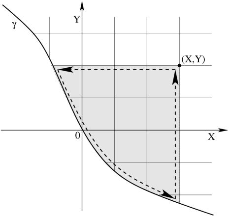
Figure 2: The closed curve $\Sigma$

Integrating along $\Sigma$, recalling that $p=q=1$ along $\gamma$ and then using (2.29), we obtain

$$\begin{array}[]{rcl}\int_{\varphi^{-1}(Y)}^{X}p(X^{\prime},Y)\,dX^{\prime}+\int_{\varphi(X)}^{Y}q(X,Y^{\prime})\,dY^{\prime}&=&X-\varphi^{-1}(Y)+Y-\varphi(X)\\[11.38109pt] &\leq&2(|X|+|Y|+4{\cal E}_{0})\,.\end{array}$$ (3.2)

Using (3.1)-(3.2) in (2.25), since $p,q>0$ we obtain the a priori bounds

$$\begin{array}[]{rcl}p(X,Y)&=&\exp\left\{\int_{\varphi(X)}^{Y}{c^{\prime}(u)\over 8c^{2}(u)}\,\big{[}\sin z-\sin w\big{]}\,q(X,Y^{\prime})\,dY^{\prime}\right\}\\[11.38109pt] &\leq&\exp\left\{C_{0}\,\int_{\varphi(X)}^{Y}\,q(X,Y^{\prime})\,dY^{\prime}\right\}\\[11.38109pt] &\leq&\exp\big{\{}2C_{0}(|X|+|Y|+4{\cal E}_{0})\big{\}}\,.\end{array}$$ (3.3)

Similarly,

$$q(X,Y)\leq\exp\big{\{}2C_{0}(|X|+|Y|+4{\cal E}_{0})\big{\}}\,.$$ (3.4)

Relying on (3.3)-(3.4), we now show that, on bounded sets in the $X$-$Y$ plane, the solution of (2.24)–(2.26) with boundary conditions (2.31) can be obtained as the fixed point of a contractive transformation. For any given $r>0$, consider the bounded domain

$$\Omega_{r}\doteq\big{\{}(X,Y)\,;~{}~{}Y\geq\varphi(X)\,,\quad X\leq r\,,\quad Y\leq r\big{\}}\,.$$

Introduce the space of functions

$$\Lambda_{r}\doteq\Big{\{}f:\Omega_{r}\mapsto{\mathbb{R}}\,;~{}~{}\|f\|_{*}\doteq{\rm ess}\!\!\sup_{(X,Y)\in\Omega_{r}}~{}e^{-\kappa(X+Y)}\big{|}f(X,Y)\big{|}~{}<~{}\infty\Big{\}}$$

where $\kappa$ is a suitably large constant, to be determined later. For $w,z,p,q,u\in\Lambda_{r}$, consider the transformation ${\cal T}(w,z,p,q,u)=(\tilde{w},\tilde{z},\tilde{p},\tilde{q},\tilde{u})$ defined by

$$\left\{\begin{array}[]{rcl}\tilde{w}(X,Y)&=&\bar{w}(X,\varphi(X))+\int_{\varphi(X)}^{Y}{c^{\prime}(u)\over 8c^{2}(u)}\,(\cos z-\cos w)\,q\,dY,\\[11.38109pt] \tilde{z}(X,Y)&=&\bar{z}(\varphi^{-1}(Y),Y)+\int_{\varphi^{-1}(Y)}^{X}{c^{\prime}(u)\over 8c^{2}(u)}\,(\cos w-\cos z)\,p\,dX\,,\end{array}\right.$$ (3.5)

$$\left\{\begin{array}[]{rcl}\tilde{p}(X,Y)&=&1+\int_{\varphi(X)}^{Y}{c^{\prime}(u)\over 8c^{2}(u)}\,\big{[}\sin z-\sin w\big{]}\,\hat{p}\hat{q}\,dY\},\\[11.38109pt] \tilde{q}(X,Y)&=&1+\int_{\varphi^{-1}(Y)}^{X}{c^{\prime}(u)\over 8c^{2}(u)}\,\big{[}\sin w-\sin z\big{]}\,\hat{p}\hat{q}\,dX\}\,,\end{array}\right.$$ (3.6)

$$\tilde{u}(X,Y)=\bar{u}(X,\varphi(X))+\int_{\varphi(X)}^{Y}{\sin z\over 4c}\,q\,dY.$$ (3.7)

In (3.6), the quantities $\hat{p},\hat{q}$ are defined as

$$\hat{p}\doteq\min\big{\{}p\,,~{}2e^{2C_{0}(|X|+|Y|+4{\cal E}_{0})}\big{\}}\,,\qquad\qquad\hat{q}\doteq\min\big{\{}q\,,~{}2e^{2C_{0}(|X|+|Y|+4{\cal E}_{0})}\big{\}}\,.$$ (3.8)

Notice that $\hat{p}=p$, $\hat{q}=q$ as long as the a priori estimates (3.3)-(3.4) are satisfied. Moreover, if in the equations (2.24)– (2.26) the variables $p,q$ are replaced with $\hat{p},\hat{q}$, then the right hand sides become uniformly Lipschitz continuous on bounded sets in the $X$-$Y$ plane. A straightforward computation now shows that the map ${\cal T}$ is a strict contraction on the space $\Lambda_{r}$, provided that the constant $\kappa$ is chosen sufficiently big (depending on the function $c$ and on $r$).

Obviously, if $r^{\prime}>r$, then the solution of (3.5)–(3.7) on $\Omega_{r^{\prime}}$ also provides the solution to the same equations on $\Omega_{r}$, when restricted to this smaller domain. Letting $r\to\infty$, in the limit we thus obtain a unique solution $(w,z,p,q,u)$ of (3.5)–(3.7), defined on the whole domain $\Omega^{+}$.

To prove that these functions satisfy the (2.24)–(2.26), we claim that $\hat{p}=p$, $\hat{q}=q$ at every point $(X,Y)\in\Omega^{+}$. The proof is by contradiction. If our claim does not hold, since the maps $Y\mapsto p(X,Y)$, $X\mapsto q(X,Y)$ are continuous, we can find some point $(X^{*},Y^{*})\in\Omega^{+}$ such that

$$p(X,Y)\leq 2e^{2C_{0}(|X|+|Y|+4{\cal E}_{0})}\,,\qquad\qquad q(X,Y)\leq 2e^{2C_{0}(|X|+|Y|+4{\cal E}_{0})}$$ (3.9)

for all $(X,Y)\in\Omega^{*}\doteq\Omega^{+}\cap\{X\leq X^{*}\,,~{}~{}Y\leq Y^{*}\}$, but either $p(X^{*},Y^{*})\geq{3\over 2}e^{2C_{0}(|X|+|Y|+4{\cal E}_{0})}$ or $q(X^{*},Y^{*})\geq{3\over 2}e^{2C_{0}(|X|+|Y|+4{\cal E}_{0})}$. By (3.9), we still have $\hat{p}=p$, $\hat{q}=q$ restricted to $\Omega^{*}$, hence the equations (2.24)–(2.26) and the a priori bounds (3.3)-(3.4) remain valid. In particular, these imply

$$p(X^{*},Y^{*})\leq e^{2C_{0}(|X|+|Y|+4{\cal E}_{0})}\,,\qquad\qquad q(X^{*},Y^{*})\leq e^{2C_{0}(|X|+|Y|+4{\cal E}_{0})}\,,$$

reaching a contradiction. MM     

Remark 3. In the solution constructed above, the variables $w,z$ may well grow outside the initial range $\,]-\pi,\pi[\,$. This happens precisely when the quantities $R$, $S$ become unbounded, i.e. when singularities arise. For future reference, we state a useful consequence of the above construction. Corollary 1. If the initial data $u_{0},u_{1}$ are smooth, then the solution $(u,p,q,w,z)$ of (2.24)–(2.26), (2.31) is a smooth function of the variables $(X,Y)$. Moreover, assume that a sequence of smooth functions $(u_{0}^{m},u_{1}^{m})_{m\geq 1}$ satisfies

$$u_{0}^{m}\to u_{0}\,,\qquad(u_{0}^{m})_{x}\to(u_{0})_{x}\,,\qquad u_{1}^{m}\to u_{1}$$

uniformly on compact subsets of ${\mathbb{R}}$. Then one has the convergence of the corresponding solutions:

$$(u^{m},\,p^{m},\,q^{m},\,w^{m},\,z^{m})\to(u,p,q,w,z)$$

uniformly on bounded subsets of the $X$-$Y$ plane. We also remark that the equations (2.24)–(2.26) imply the conservation laws

$$q_{X}+p_{Y}=0\,,\qquad\qquad\left({q\over c}\right)_{X}-\left({p\over c}\right)_{Y}=0\,.$$ (3.10)

4 Weak solutions, in the original variables

By expressing the solution $u(X,Y)$ in terms of the original variables $(t,x)$, we shall recover a solution of the Cauchy problem (1.1)-(1.2). This will provide a proof of Theorem 1.

As a preliminary, we examine the regularity of the solution $(u,w,z,p,q)$ constructed in the previous section. Since the initial data $(u_{0})_{x}$ and $u_{1}$ are only assumed to be in ${\bf L}^{2}$, the functions $w,z,p,q$ may well be discontinuous. More precisely, on bounded subsets of the $X$-$Y$ plane, the equations (2.24)-(2.26) imply the following:

-

The functions $w,p$ are Lipschitz continuous w.r.t. $Y$, measurable w.r.t. $X$.

-

The functions $z,q$ are Lipschitz continuous w.r.t. $X$, measurable w.r.t. $Y$.

-

The function $u$ is Lipschitz continuous w.r.t. both $X$ and $Y$.

The map $(X,Y)\mapsto(t,x)$ can be constructed as follows. Setting $f=x$, then $f=t$ in the two equations at (2.16), we find

$$\left\{\begin{array}[]{rcr}c&=&2cX_{x}\,x_{X}\,,\\[8.53581pt] -c&=&-2cY_{x}\,x_{Y}\,,\end{array}\right.\qquad\qquad\left\{\begin{array}[]{rcr}1&=&2cX_{x}\,t_{X}\,,\\[8.53581pt] 1&=&-2cY_{x}\,t_{Y}\,,\end{array}\right.$$

respectively. Therefore, using (2.18) we obtain

$$\left\{\begin{array}[]{ccccr}x_{X}&~{}={}&{1\over 2X_{x}}&~{}={}&{(1+\cos w)\,p\over 4}\,,\\[11.38109pt] x_{Y}&~{}={}&{1\over 2Y_{x}}&~{}={}&-{(1+\cos z)\,q\over 4}\,,\end{array}\right.$$ (4.1)

$$\left\{\begin{array}[]{ccccr}t_{X}&=&{1\over 2cX_{x}}&=&{(1+\cos w)\,p\over 4c}\,,\\[11.38109pt] t_{Y}&=&{1\over-2cY_{x}}&=&{(1+\cos z)\,q\over 4c}\,.\end{array}\right.$$ (4.2)

For future reference, we write here the partial derivatives of the inverse mapping, valid at points where $w,z\not=-\pi$.

$$\left\{\begin{array}[]{ccr}X_{x}&=&{2\over(1+\cos w)\,p}\,,\\[11.38109pt] Y_{x}&=&\,-{2\over(1+\cos z)\,q}\,,\end{array}\right.\qquad\qquad\left\{\begin{array}[]{ccr}X_{t}&=&{2c\over(1+\cos w)\,p}\,,\\[11.38109pt] Y_{t}&=&{2c\over(1+\cos z)\,q}\,.\end{array}\right.$$ (4.3)

We can now recover the functions $x=x(X,Y)$ by integrating one of the equations in (4.1). Moreover, we can compute $t=t(X,Y)$ by integrating one of the equations in (4.2). A straightforward calculation shows that the two equations in (4.1) are equivalent: differentiating the first w.r.t. $Y$ or the second w.r.t. $X$ one obtains the same expression.

$$\begin{array}[]{ccl}x_{XY}&=&{(1+\cos w)\,p_{Y}\over 4}-{p\sin w\,w_{Y}\over 4}\\[8.53581pt] &=&{c^{\prime}\,pq\over 32c^{2}}\,\big{[}\sin z-\sin w+\sin(z-w)\big{]}=x_{Y\!X}\,.\end{array}$$

Similarly, the equivalence of the two equations in (4.2) is checked by

$$\begin{array}[]{cl}&t_{XY}-t_{Y\!X}~{}=~{}\left({x_{X}\over c}\right)_{Y}+\left({x_{Y}\over c}\right)_{X}~{}=~{}{2\over c}\,x_{XY}-\left({x_{X}\over c^{2}}\,c^{\prime}u_{Y}+{x_{Y}\over c^{2}}\,c^{\prime}u_{X}\right)\\[8.53581pt] &\quad={c^{\prime}\,pq\over 16\,c^{3}}\,\big{[}\sin z-\sin w+\sin(z-w)\big{]}\\[8.53581pt] &\qquad\qquad-{c^{\prime}\,pq\over 16\,c^{3}}\big{[}(1+\cos w)\sin z-(1+\cos z)\sin w\big{]}~{}=~{}0\,.\end{array}$$

In order to define $u$ as a function of the original variables $t,x$, we should formally invert the map $(X,Y)\mapsto(t,x)$ and write $u(t,x)=u\big{(}X(t,x)\,,~{}Y(t,x)\big{)}$. The fact that the above map may not be one-to-one does not cause any real difficulty. Indeed, given $(t^{*},x^{*})$, we can choose an arbitrary point $(X^{*},Y^{*})$ such that $t(X^{*},Y^{*})=t^{*}$, $x(X^{*},Y^{*})=x^{*}$, and define $u(t^{*},x^{*})=u(X^{*},Y^{*})$. To prove that the values of $u$ do not depend on the choice of $(X^{*},Y^{*})$, we proceed as follows. Assume that there are two distinct points such that $t(X_{1},Y_{1})=t(X_{2},Y_{2})=t^{*}$, $~{}x(X_{1},Y_{1})=x(X_{2},Y_{2})=x^{*}$. We consider two cases: Case 1: $X_{1}\leq X_{2}$, $Y_{1}\leq Y_{2}$. Consider the set

$$\Gamma_{x^{*}}\doteq\Big{\{}(X,Y)\,;~{}~{}x(X,Y)\leq x^{*}\Big{\}}$$

and call $\partial\Gamma_{x^{*}}$ its boundary. By (4.1), $x$ is increasing with $X$ and decreasing with $Y$. Hence, this boundary can be represented as the graph of a Lipschitz continuous function: $X-Y=\phi(X+Y)$. We now construct the Lipschitz continuous curve $\gamma$ (fig. 3a) consisting of

-

a horizontal segment joining $(X_{1},Y_{1})$ with a point $A=(X_{A},Y_{A})$ on $\partial\Gamma_{x^{*}}$, with $Y_{A}=Y_{1}$,

-

a portion of the boundary $\partial\Gamma_{x^{*}}$,

-

a vertical segment joining $(X_{2},Y_{2})$ to a point $B=(X_{B},Y_{B})$ on $\partial\Gamma_{x^{*}}$, with $X_{B}=X_{2}$.

We can obtain a Lipschitz continuous parametrization of the curve $\gamma:[\xi_{1},\xi_{2}]\mapsto{\mathbb{R}}^{2}$ in terms of the parameter $\xi=X+Y$. Observe that the map $(X,Y)\mapsto(t,x)$ is constant along $\gamma$. By (4.1)-(4.2) this implies $(1+\cos w)X_{\xi}=(1+\cos z)Y_{\xi}=0$, hence $\sin w\cdot X_{\xi}=\sin z\cdot Y_{\xi}=0$. We now compute

$$\begin{array}[]{rl}u(X_{2},Y_{2})-&u(X_{1},Y_{1})=\int_{\gamma}\big{(}u_{X}\,dX+u_{Y}\,dY\big{)}\cr&=\int_{\xi_{1}}^{\xi_{2}}\left({p\,\sin w\over 4c}\,X_{\xi}-{q\,\sin z\over 4c}\,Y_{\xi}\right)\,d\xi=0\,,\end{array}$$

proving our claim. Case 2: $X_{1}\leq X_{2}$, $Y_{1}\geq Y_{2}$. In this case, we consider the set

$$\Gamma_{t^{*}}\doteq\Big{\{}(X,Y)\,;~{}~{}t(X,Y)\leq t^{*}\Big{\}}\,,$$

and construct a curve $\gamma$ connecting $(X_{1},Y_{1})$ with $(X_{2},Y_{2})$ as in fig. 3b. Details are entirely similar to Case 1.

Figure 3: Paths of integration

We now prove that the function $u(t,x)=u\big{(}X(t,x),Y(t,x)\big{)}$ thus obtained is Hölder continuous on bounded sets. Toward this goal, consider any characteristic curve, say $t\mapsto x^{+}(t)$, with $\dot{x}^{+}=c(u)$. By construction, this is parametrized by the function $X\mapsto\big{(}t(X,\overline{Y}),\,x(X,\overline{Y})\big{)}$, for some fixed $\overline{Y}$. Recalling (2.16), (2.14), (2.18) and (2.26), we compute

$$\begin{array}[]{rcl}\int_{0}^{\tau}\big{[}u_{t}+c(u)u_{x}\big{]}^{2}\,dt&=&\int_{X_{0}}^{X_{\tau}}(2cX_{x}u_{X})^{2}\,(2X_{t})^{-1}dX\\[11.38109pt] &=&\int_{X_{0}}^{X_{\tau}}2c\left(p\,\cos^{2}{w\over 2}\right)^{-1}\,\left({p\over 4c}\,2\sin{w\over 2}\cos{w\over 2}\right)^{2}\,dX\\[11.38109pt] &\leq&\int_{X_{0}}^{X_{\tau}}{p\over 2c}\,dX~{}\leq~{}C_{\tau}\,,\end{array}$$ (4.4)

for some constant $C_{\tau}$ depending only on $\tau$. Similarly, integrating along any backward characteristics $t\mapsto x^{-}(t)$ we obtain

$$\int_{0}^{\tau}\big{[}u_{t}-c(u)u_{x}\big{]}^{2}\,dt\leq C_{\tau}.$$ (4.5)

Since the speed of characteristics is $\pm c(u)$, and $c(u)$ is uniformly positive and bounded, the bounds (4.4)-(4.5) imply that the function $u=u(t,x)$ is Hölder continuous with exponent $1/2$. In turn, this implies that all characteristic curves are ${\cal C}^{1}$ with Hölder continuous derivative. Still from (4.4)-(4.5) it follows that the functions $R,S$ at (2.1) are square integrable on bounded subsets of the $t$-$x$ plane. Finally, we prove that the function $u$ provides a weak solution to the nonlinear wave equation (1.1). According to (1.5), we need to show that

$$\begin{array}[]{rcl}0&=&\int\!\!\int\phi_{t}\big{[}(u_{t}+cu_{x})+(u_{t}-cu_{x})\big{]}-\big{(}c(u)\phi\big{)}_{x}\big{[}(u_{t}+cu_{x})-(u_{t}-cu_{x})\big{]}\,dxdt\\[11.38109pt] &=&\int\!\!\int\big{[}\phi_{t}-(c\phi)_{x}\big{]}\,(u_{t}+cu_{x})\,dxdt+\int\!\!\int\big{[}\phi_{t}+(c\phi)_{x}\big{]}\,(u_{t}-cu_{x})\,dxdt\\[11.38109pt] &=&\int\!\!\int\big{[}\phi_{t}-(c\phi)_{x}\big{]}\,R\,dxdt+\int\!\!\int\big{[}\phi_{t}+(c\phi)_{x}\big{]}\,S\,dxdt\,.\end{array}$$ (4.6)

By (2.16), this is equivalent to

$$\int\!\!\int\Big{\{}-2cY_{x}\phi_{Y}\,R~{}+~{}2cX_{x}\phi_{X}\,S~{}+~{}c^{\prime}(u_{X}\,X_{x}+u_{Y}\,Y_{x})\,\phi\,(S-R)\Big{\}}\,dxdt=0\,.$$ (4.7)

It will be convenient to express the double integral in (4.7) in terms of the variables $X,Y$. We notice that, by (2.18) and (2.14),

$$dx\,dt={pq\over 2c\,(1+R^{2})(1+S^{2})}\,dXdY\,.$$

Using (2.26) and the identities

$$\left\{\begin{array}[]{ccc}{1\over 1+R^{2}}&=&\cos^{2}{w\over 2}={1+\cos w\over 2}\,,\\[11.38109pt] {1\over 1+S^{2}}&=&\cos^{2}{z\over 2}={1+\cos z\over 2}\,,\end{array}\right.\qquad\qquad\left\{\begin{array}[]{ccc}{R\over 1+R^{2}}&=&{\sin w\over 2}\,,\\[11.38109pt] {S\over 1+S^{2}}&=&{\sin z\over 2}\,,\end{array}\right.$$ (4.8)

the double integral in (4.6) can thus be written as

$$\begin{array}[]{rl}\int\!\!\int&\left\{2c\,{1+S^{2}\over q}\,\phi_{Y}\,R+2c{1+R^{2}\over p}\,\phi_{X}\,S+c^{\prime}\left({\sin w\over 4c}\,p\,{1+R^{2}\over p}-{\sin z\over 4c}\,q\,{1+S^{2}\over q}\right)\,\phi\,(S-R)\right\}\\[11.38109pt] &\qquad\qquad\cdot{pq\over 2c\,(1+R^{2})\,(1+S^{2})}\,dXdY\\[11.38109pt] &=\int\!\!\int\left\{{R\over 1+R^{2}}\,p\,\phi_{Y}+{S\over 1+S^{2}}\,q\,\phi_{X}+{c^{\prime}pq\over 8c^{2}}\left({\sin w\over 1+S^{2}}-{\sin z\over 1+R^{2}}\right)\phi\,(S-R)\right\}\,dXdY\\[11.38109pt] &=\int\!\!\int\bigg{\{}{p\,\sin w\over 2}\,\phi_{Y}+{q\sin z\over 2}\,\phi_{X}\\[11.38109pt] &\qquad+{c^{\prime}pq\over 8c^{2}}\left(\sin w\sin z-\sin w\,\cos^{2}{z\over 2}\tan{w\over 2}-\sin z\,\cos^{2}{w\over 2}\,\tan{z\over 2}\right)\,\phi\bigg{\}}\,dXdY\\[11.38109pt] &=\int\!\!\int\left\{{p\,\sin w\over 2}\,\phi_{Y}+{q\sin z\over 2}\,\phi_{X}+{c^{\prime}pq\over 8c^{2}}\,\big{[}\cos(w+z)-1\big{]}\,\phi\right\}\,dXdY\,.\end{array}$$ (4.9)

Recalling (2.30), one finds

$$\begin{array}[]{rcl}\left(p\,\sin w\over 2\right)_{Y}+\left(q\,\sin z\over 2\right)_{X}&=&(2c\,u_{X})_{Y}+(2c\,u_{Y})_{X}\\[11.38109pt] &=&4c^{\prime}u_{X}u_{Y}+4c\,u_{XY}\\[11.38109pt] &=&{c^{\prime}\,pq\over 4c^{2}}\,\sin w\,\sin z+{c^{\prime}\,pq\over 8c^{2}}\,\big{[}\cos(w-z)-1\big{]}\\[11.38109pt] &=&{c^{\prime}\,pq\over 8c^{2}}\big{[}\cos(w+z)-1\big{]}\,.\end{array}$$ (4.10)

Together, (4.9) and (4.10) imply (4.7) and hence (4.6). This establishes the integral equation (1.5) for every test function $\phi\in{\cal C}^{1}_{c}$.

5 Conserved quantities

From the conservation laws (3.10) it follows that the 1-forms $p\,dX-q\,dY$ and $\frac{p}{c}\,dX+\frac{q}{c}\,dY$ are closed, hence their integrals along any closed curve in th $X$-$Y$ plane vanish. From the conservation laws at (2.6), it follows that the 1-forms

$$E\,dx-(c^{2}M)\,dt\,,\qquad\qquad M\,dx-E\,dt$$ (5.1)

are also closed. There is a simple correspondence. In fact

$$E\,dx-(c^{2}M)\,dt=\frac{p}{4}\,dX-\frac{q}{4}\,dY-\frac{1}{2}\,dx\quad-M\,dx+E\,dt=\frac{p}{4c}\,dX+\frac{q}{4c}\,dY-\frac{1}{2}\,dt.$$

Recalling (4.1)-(4.2), these can be written in terms of the $X$-$Y$ coordinates as

$${(1-\cos w)\,p\over 8}\,dX-{(1-\cos z)\,q\over 8}\,dY\,,$$ (5.2)

$${(1-\cos w)\,p\over 8c}\,dX+{(1-\cos z)\,q\over 8c}\,dY\,,$$ (5.3)

respectively. Using (2.24)–(2.26), one easily checks that these forms are indeed closed:

$$\left({(1-\cos w)\,p\over 8}\right)_{Y}={c^{\prime}pq\over 64c^{2}}\Big{[}\sin z(1-\cos w)-\sin w(1-\cos z)\Big{]}=-\left({(1-\cos z)\,q\over 8}\right)_{X}\,,$$ (5.4)

$$\left({(1-\cos w)\,p\over 8c}\right)_{Y}={c^{\prime}pq\over 64c^{3}}\Big{[}\sin(w+z)-(\sin w+\sin z)\Big{]}=\left({(1-\cos z)\,q\over 8c}\right)_{X}\,.$$

In addition, we have the 1-forms

$$dx={(1+\cos w)\,p\over 4}\,dX-{(1+\cos z)\,q\over 4}\,dY\,,$$ (5.5)

$$dt={(1+\cos w)\,p\over 4c}\,dX+{(1+\cos z)\,q\over 4c}\,dY\,,$$ (5.6)

which are obviously closed.

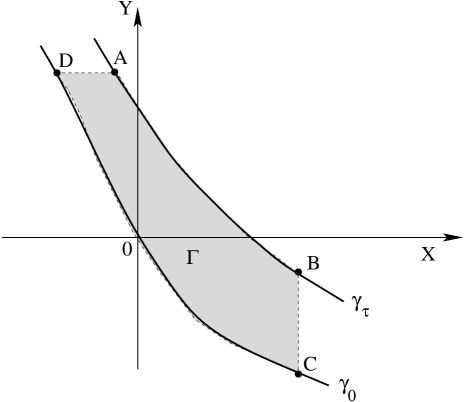
Figure 4:

The solutions $u=u(X,Y)$ constructed in Section 3 are conservative, in the sense that the integral of the form (5.2) along every Lipschitz continuous, closed curve in the $X$-$Y$ plane is zero.

To prove the inequality (1.7), fix any $\tau>0$. The case $\tau<0$ is identical. For a given $r>0$ arbitrarily large, define the set (fig. 4)

$$\Gamma\doteq\Big{\{}(X,Y)\,;~{}~{}0\leq t(X,Y)\leq\tau\,,\quad X\leq r\,,~{}~{}Y\leq r\Big{\}}$$ (5.7)

By construction, the the map $(X,Y)\mapsto(t,x)$ will act as follows:

$$A\mapsto(\tau,a)\,,\qquad B\mapsto(\tau,b)\,,\qquad C\mapsto(0,c)\,,\qquad D\mapsto(0,d)\,,$$

for some $a<b$ and $d<c$. Integrating the 1-form (5.2) along the boundary of $\Gamma$ we obtain

$$\begin{array}[]{rl}\int_{AB}&{(1-\cos w)\,p\over 8}\,dX-{(1-\cos z)\,q\over 8}\,dY\\[11.38109pt] &=\int_{DC}{(1-\cos w)\,p\over 8}\,dX-{(1-\cos z)\,q\over 8}\,dY\,-\int_{DA}{(1-\cos w)\,p\over 8}\,dX-\int_{CB}{(1-\cos z)\,q\over 8}\,dY\\[11.38109pt] &\leq\int_{DC}{(1-\cos w)\,p\over 8}\,dX-{(1-\cos z)\,q\over 8}\,dY\\[11.38109pt] &=\int_{d}^{c}\frac{1}{2}\Big{[}u_{t}^{2}(0,x)+c^{2}\big{(}u(0,x)\big{)}\,u_{x}^{2}(0,x)\Big{]}\,dx\,.\end{array}$$ (5.8)

On the other hand, using (5.5) we compute

$$\begin{array}[]{rl}\int_{a}^{b}\frac{1}{2}\Big{[}u_{t}^{2}(\tau,x)+&c^{2}\big{(}u(\tau,x)\big{)}\,u_{x}^{2}(\tau,x)\big{]}\,dx\\[11.38109pt] &=\int_{AB\cap\{\cos w\not=-1\}}{(1-\cos w)\,p\over 8}\,dX+\int_{AB\cap\{\cos z\not=-1\}}{(1-\cos z)\,q\over 8}\,dY\\[11.38109pt] &\leq{\cal E}_{0}\,.\end{array}$$ (5.9)

Notice that the last relation in (5.8) is satisfied as an equality, because at time $t=0$, along the curve $\gamma_{0}$ the variables $w,z$ never assume the value $-\pi$. Letting $r\to+\infty$ in (5.7), one has $a\to-\infty$, $b\to+\infty$. Therefore (5.8) and (5.9) together imply ${\cal E}(t)\leq{\cal E}_{0}$, proving (1.7).

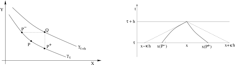
Figure 5: Proving Lipschitz continuity

We now prove the Lipschitz continuity of the map $t\mapsto u(t,\cdot)$ in the ${\bf L}^{2}$ distance. For this purpose, for any fixed time $\tau$, we let $\mu_{\tau}=\mu_{\tau}^{-}+\mu_{\tau}^{+}$ be the positive measure on the real line defined as follows. In the smooth case,

$$\mu_{\tau}^{-}\big{(}\,]a,b[\,\big{)}=\frac{1}{4}\int_{a}^{b}R^{2}(\tau,x)\,dx\,,\qquad\qquad\mu_{\tau}^{+}\big{(}\,]a,b[\,\big{)}=\frac{1}{4}\int_{a}^{b}S^{2}(\tau,x)\,dx\,.$$ (5.10)

To define $\mu_{\tau}^{\pm}$ in the general case, let $\gamma_{\tau}$ be the boundary of the set

$$\Gamma_{\tau}\doteq\big{\{}(X,Y)\,;~{}~{}t(X,Y)\leq\tau\big{\}}\,.$$ (5.11)

Given any open interval $]a,b[\,$, let $A=(X_{A},Y_{A})$ and $B=(X_{B},Y_{B})$ be the points on $\gamma_{\tau}$ such that

$$x(A)=a\,,\qquad X_{P}-Y_{P}\leq X_{A}-Y_{A}\quad\hbox{for every point $P\in\gamma_{\tau}$ with $x(P)\leq a$}\,,$$

$$x(B)=b\,,\qquad X_{P}-Y_{P}\geq X_{B}-Y_{B}\quad\hbox{for every point $P\in\gamma_{\tau}$ with $x(P)\geq b$}\,.$$

Then

$$\mu_{\tau}\big{(}\,]a,b[\,\big{)}=\mu_{\tau}^{-}\big{(}\,]a,b[\,\big{)}+\mu_{\tau}^{+}\big{(}\,]a,b[\,\big{)}\,,$$ (5.12)

where

$$\mu_{\tau}^{-}\big{(}\,]a,b[\,\big{)}\doteq\int_{AB}{(1-\cos w)\,p\over 8}\,dX\,\qquad\mu_{\tau}^{+}\big{(}\,]a,b[\,\big{)}\doteq-\int_{AB}{(1-\cos z)\,q\over 8}\,dY\,.$$ (5.13)

Recalling the discussion at (5.1)–(5.2), it is clear that $\mu_{\tau}^{-}$, $\mu_{\tau}^{+}$ are bounded, positive measures, and $\mu_{\tau}({\mathbb{R}})={\cal E}_{0}$, for all $\tau$. Moreover, by (5.10) and (2.5),

$$\int_{a}^{b}c^{2}u_{x}^{2}\,dx\leq\int_{a}^{b}\frac{1}{2}(R^{2}+S^{2})dx\leq 2\mu(]a,b[).$$

For any $a<b$, this yields the estimate

$$|u(\tau,b)-u(\tau,a)|^{2}\leq|b-a|\int_{a}^{b}u_{x}^{2}(\tau,y)\,dy\leq 2\kappa^{2}|b-a|\mu_{\tau}(]a,b[).$$ (5.14)

Next, for a given $h>0$, $y\in{\mathbb{R}}$, we seek an estimate on the distance $\big{|}u(\tau+h,\,y)-u(\tau,y)|$. As in fig. 5, let $\gamma_{\tau+h}$ be the boundary of the set $\Gamma_{\tau+h}$, as in (5.11). Let $P=(P_{X},\,P_{Y})$ be the point on $\gamma_{\tau}$ such that

$$x(P)=y\,,\qquad X_{P^{\prime}}-Y_{P^{\prime}}\leq X_{P}-Y_{P}\quad\hbox{for every point $P^{\prime}\in\gamma_{\tau}$ with $x(P^{\prime})\leq x$}\,,$$

Similarly, let $Q=(Q_{X},\,Q_{Y})$ be the point on $\gamma_{\tau+h}$ such that

$$x(Q)=y\,,\qquad X_{Q^{\prime}}-Y_{Q^{\prime}}\leq X_{Q}-Y_{Q}\quad\hbox{for every point $Q^{\prime}\in\gamma_{\tau+h}$ with $x(Q^{\prime})\leq y$}\,.$$

Notice that $X_{P}\leq X_{Q}$ and $Y_{P}\leq Y_{Q}$. Let $P^{+}=(X^{+},Y^{+})$ be a point on $\gamma_{\tau}$ with $X^{+}=X_{Q}$, and let $P^{-}=(X^{-},Y^{-})$ be a point on $\gamma_{\tau}$ with $Y^{-}=Y_{Q}$. Notice that $x(P^{+})\in\,]y,\,y+\kappa h[\,$, because the point $\big{(}\tau,x(Q)\big{)}$ lies on some characteristic curve with speed $-c(u)>-\kappa$, passing through the point $(\tau+h,\,y)$. Similarly, $x(P^{-})\in\,]y-\kappa h,\,y[\,$. Recalling that the forms in (5.2) and (5.6) are closed, we obtain the estimate

$$\begin{array}[]{rcl}\big{|}u(Q)-u(P^{+})\big{|}&\leq&\int_{Y^{+}}^{Y_{Q}}\big{|}u_{Y}(X_{Q},Y)\big{|}\,dY\\[11.38109pt] &=&\int_{Y^{+}}^{Y_{Q}}\left|{\sin z\over 4c}\,q\right|\,dY\\[11.38109pt] &=&\int_{Y^{+}}^{Y_{Q}}\left({(1+\cos z)\,q\over 4c}\right)^{1/2}\left({(1-\cos z)\,q\over 4}\right)^{1/2}\,dY\\[11.38109pt] &\leq&\left(\int_{Y^{+}}^{Y_{Q}}{(1+\cos z)\,q\over 4c}\,dY\right)^{1/2}\cdot\left(\int_{Y^{+}}^{Y_{Q}}{(1-\cos z)\,q\over 4}\,dY\right)^{1/2}\\[11.38109pt] &\leq&\left\{\int_{P^{-}P^{+}}\left[{(1-\cos w)\,p\over 4}\,dX-{(1-\cos z)\,q\over 4}\,dY\right]\right\}^{1/2}\cdot h^{1/2}\,.\end{array}$$ (5.15)

The last term in (5.15) contains the integral of the 1-form at (5.2), along the curve $\gamma_{\tau}$, between $P^{-}$ and $P^{+}$. Recalling the definition (5.12)–(5.13) and the estimate (5.14), we obtain the bound

$$\begin{array}[]{rcl}\big{|}u(\tau+h,x)-u(\tau,x)\big{|}^{2}&\leq&2\big{|}u(Q)-u(P^{+})\big{|}^{2}+2\big{|}u(P^{+})-u(P)\big{|}^{2}\\[8.53581pt] &\leq&4h\cdot\mu_{\tau}\big{(}]x-\kappa h,\,x+\kappa h[\big{)}+4\kappa^{2}\cdot(\kappa h)\cdot\mu_{\tau}\big{(}]x\,,~{}x+h[\big{)}\,.\end{array}$$ (5.16)

Therefore, for any $h>0$,

$$\begin{array}[]{rcl}\big{\|}u(\tau+h,\cdot)-u(\tau,\cdot)\big{\|}_{{\bf L}^{2}}&=&\left(\int\big{|}u(\tau+h,x)-u(\tau,x)\big{|}^{2}\,dx\right)^{1/2}\\[11.38109pt] &\leq&\left(\int 4(1+\kappa^{3})h\cdot\mu_{\tau}\big{(}]x-\kappa h\,,~{}x+\kappa h[\big{)}\,dx\right)^{1/2}\\[11.38109pt] &=&\Big{(}4(\kappa^{3}+1)h^{2}\,\mu_{\tau}({\mathbb{R}})\Big{)}^{1/2}\\[11.38109pt] &=&h\cdot\big{[}4(\kappa^{3}+1)\,{\cal E}_{0}\big{]}^{1/2}.\end{array}$$ (5.17)

This proves the uniform Lipschitz continuity of the map $t\mapsto u(t,\cdot)$, stated at (1.4).

6 Regularity of trajectories

In this section we prove the continuity of the functions $t\mapsto u_{t}(t,\cdot)$ and $t\mapsto u_{x}(t,\cdot)$, as functions with values in ${\bf L}^{p}$. This will complete the proof of Theorem 1.

We first consider the case where the initial data $(u_{0})_{x}$, $u_{1}$ are smooth with compact support. In this case, the solution $u=u(X,Y)$ remains smooth on the entire $X$-$Y$ plane. Fix a time $\tau$ and let $\gamma_{\tau}$ be the boundary of the set $\Gamma_{\tau}$, as in (5.11). We claim that

$${d\over dt}u(t,\cdot)\bigg{|}_{t=\tau}=u_{t}(\tau,\cdot)$$ (6.1)

where, by (2.14), (2.18) and (2.26),

$$\begin{array}[]{rcl}u_{t}(\tau,x)&\doteq&u_{X}\,X_{t}+u_{Y}\,Y_{t}\\[11.38109pt] &=&{p\,\sin w\over 4c}\,{2c\over p(1+\cos w)}+{q\,\sin z\over 4c}\,{2c\over q(1+\cos z)}={\sin w\over 2(1+\cos w)}+{\sin z\over 2(1+\cos z)}\,.\end{array}$$ (6.2)

Notice that (6.2) defines the values of $u_{t}(\tau,\cdot)$ at almost every point $x\in{\mathbb{R}}$, i.e. at all points outside the support of the singular part of the measure $\mu_{\tau}$ defined at (5.12). By the inequality (1.7), recalling that $c(u)\geq\kappa^{-1}$, we obtain

$$\int_{\mathbb{R}}\big{|}u_{t}(\tau,x)\big{|}^{2}\,dx\leq\kappa^{2}\,{\cal E}(\tau)\leq\kappa^{2}{\cal E}_{0}.$$ (6.3)

To prove (6.1), let any $\varepsilon>0$ be given. There exist finitely many disjoint intervals $[a_{i},\,b_{i}]\subset{\mathbb{R}}$, $i=1,\ldots,N$, with the following property. Call $A_{i},B_{i}$ the points on $\gamma_{\tau}$ such that $x(A_{i})=a_{i}$, $x(B_{i})=b_{i}$. Then one has

$$\min\big{\{}1+\cos w(P)\,,~{}1+\cos z(P)\big{\}}<2\varepsilon$$ (6.4)

at every point $P$ on $\gamma_{\tau}$ contained in one of the arcs $A_{i}B_{i}$, while

$$1+\cos w(P)>\varepsilon\,,\qquad\qquad 1+\cos z(P)>\varepsilon\,,$$ (6.5)

for every point $P$ along $\gamma_{\tau}$, not contained in any of the arcs $A_{i}B_{i}$. Call $J\doteq\cup_{1\leq i\leq N}[a_{i},b_{i}]$, $J^{\prime}={\mathbb{R}}\setminus J$, and notice that, as a function of the original variables, $u=u(t,x)$ is smooth in a neighborhood of the set $\{\tau\}\times J^{\prime}$. Using Minkowski’s inequality and the differentiability of $u$ on $J^{\prime}$, we can write

$$\begin{array}[]{rl}\lim_{h\to 0}&{1\over h}\left(\int_{{\mathbb{R}}}\Big{|}u(\tau+h,x)-u(\tau,x)-h\,u_{t}(\tau,x)\Big{|}^{p}dx\right)^{1/p}\\[11.38109pt] &\leq\lim_{h\to 0}{1\over h}\left(\int_{J}\Big{|}u(\tau+h,x)-u(\tau,x)\Big{|}^{p}dx\right)^{1/p}+\left(\int_{J}\big{|}u_{t}(\tau,x)\big{|}^{p}\,dx\right)^{1/p}\end{array}$$ (6.6)

We now provide an estimate on the measure of the “bad” set $J$:

$$\begin{array}[]{rcl}\hbox{meas}\,(J)&=&\int_{J}dx=\sum_{i}\int_{A_{i}B_{i}}{(1+\cos w)\,p\over 4}\,dX-{(1+\cos z)\,q\over 4}\,dY\\[11.38109pt] &\leq&2\varepsilon\sum_{i}\int_{A_{i}B_{i}}{(1-\cos w)\,p\over 4}\,dX-{(1-\cos z)\,q\over 4}\,dY\\[11.38109pt] &\leq&2\varepsilon\int_{\gamma_{\tau}}{(1-\cos w)\,p\over 4}\,dX-{(1-\cos z)\,q\over 4}\,dY\leq 2\varepsilon\,{\cal E}_{0}\,.\end{array}$$ (6.7)

Now choose $q=2/(2-p)$ so that ${p\over 2}+{1\over q}=1$. Using Hölder’s inequality with conjugate exponents $2/p$ and $q$, and recalling (5.17), we obtain

$$\begin{array}[]{rcl}\int_{J}\Big{|}u(\tau+h,x)-u(\tau,x)\Big{|}^{p}dx&\leq&\hbox{meas}\,(J)^{1/q}\cdot\left(\int_{J}\Big{|}u(\tau+h,x)-u(\tau,x)\Big{|}^{2}dx\right)^{p/2}\\[11.38109pt] &\leq&\big{[}2\varepsilon\,{\cal E}_{0}\big{]}^{1/q}\cdot\Big{(}\big{\|}u(\tau+h,\cdot)-u(\tau,\cdot)\big{\|}^{2}_{{\bf L}^{2}}\Big{)}^{p/2}\\[11.38109pt] &\leq&\big{[}2\varepsilon\,{\cal E}_{0}\big{]}^{1/q}\cdot\Big{(}h^{2}\big{[}4(\kappa^{3}+1)\,{\cal E}_{0}\big{]}\Big{)}^{p/2}.\end{array}$$

Therefore,

$$\limsup_{h\to 0}{1\over h}\left(\int_{J}\Big{|}u(\tau+h,x)-u(\tau,x)-h\Big{|}^{p}dx\right)^{1/p}\leq[2\varepsilon\,{\cal E}_{0}]^{1/pq}\cdot\big{[}4(\kappa^{3}+1)\,{\cal E}_{0}\big{]}^{1/2}.$$ (6.8)

In a similar way we estimate

$$\int_{J}\big{|}u_{t}(\tau,x)\big{|}^{p}\,dx\leq\big{[}\hbox{meas}\,(J)\big{]}^{1/q}\cdot\left(\int_{J}\Big{|}u_{t}(\tau,x)\Big{|}^{2}dx\right)^{p/2},$$

$$\left(\int_{J}\big{|}u_{t}(\tau,x)\big{|}^{p}\,dx\right)^{1/p}\leq\hbox{meas}\,(J)^{1/pq}\cdot\big{[}\kappa^{2}\,{\cal E}_{0}\big{]}^{p/2}.$$ (6.9)

Since $\varepsilon>0$ is arbitrary, from (6.6), (6.8) and (6.9) we conclude

$$\lim_{h\to 0}~{}{1\over h}\left(\int_{{\mathbb{R}}}\Big{|}u(\tau+h,x)-u(\tau,x)-h\,u_{t}(\tau,x)\Big{|}^{p}dx\right)^{1/p}=0.$$ (6.10)

The proof of continuity of the map $t\mapsto u_{t}$ is similar. Fix $\varepsilon>0$. Consider the intervals $[a_{i},b_{i}]$ as before. Since $u$ is smooth on a neighborhood of $\{\tau\}\times J^{\prime}$, it suffices to estimate

$$\begin{array}[]{cl}&\limsup_{h\to 0}\,\int\big{|}u_{t}(\tau+h,x)-u_{t}(\tau,x)\big{|}^{p}\,dx\\[11.38109pt] \leq&\limsup_{h\to 0}\int_{J}\big{|}u_{t}(\tau+h,x)-u_{t}(\tau,x)\big{|}^{p}\,dx\\[11.38109pt] \leq&\limsup_{h\to 0}\big{[}\hbox{meas}\,(J)\big{]}^{1/q}\cdot\left(\int_{J}\Big{|}u_{t}(\tau+h,\,x)-u_{t}(\tau,x)\Big{|}^{2}dx\right)^{p/2}\\[11.38109pt] \leq&\limsup_{h\to 0}\big{[}2\varepsilon\,{\cal E}_{0}\big{]}^{1/q}\cdot\Big{(}\big{\|}u_{t}(\tau+h,\cdot)\big{\|}_{{\bf L}^{2}}+\big{\|}u_{t}(\tau,\cdot)\big{\|}_{{\bf L}^{2}}\Big{)}^{p}\\[11.38109pt] \leq&\big{[}2\varepsilon{\cal E}_{0}]^{1/q}\,\big{[}4{\cal E}_{0}\big{]}^{p}.\end{array}$$

Since $\varepsilon>0$ is arbitrary, this proves continuity. To extend the result to general initial data, such that $(u_{0})_{x},u_{1}\in{\bf L}^{2}$, we consider a sequence of smooth initial data, with $(u^{\nu}_{0})_{x},u^{\nu}_{1}\in{\cal C}^{\infty}_{c}$, with $u_{0}^{n}\to u_{0}$ uniformly, $(u_{0}^{n})_{x}\to(u_{0})_{x}$ almost everywhere and in ${\bf L}^{2}$, $u_{1}^{n}\to u_{1}$ almost everywhere and in ${\bf L}^{2}$.

The continuity of the function $t\mapsto u_{x}(t,\cdot)$ as a map with values in ${\bf L}^{p}$, $1\leq p<2$, is proved in an entirely similar way.

7 Energy conservation

This section is devoted to the proof of Theorem 3, stating that, in some sense, the total energy of the solution remains constant in time.

A key tool in our analysis is the wave interaction potential, defined as

$$\Lambda(t)\doteq(\mu_{t}^{-}\otimes\mu_{t}^{+})\big{\{}(x,y)\,;~{}x>y\big{\}}\,.$$ (7.1)

We recall that $\mu_{t}^{\pm}$ are the positive measures defined at (5.13). Notice that, if $\mu_{t}^{+},\mu_{t}^{-}$ are absolutely continuous w.r.t. Lebesgue measure, so that (5.10) holds, then (7.1) is equivalent to

$$\Lambda(t)\doteq\frac{1}{4}\int\!\!\int_{x>y}R^{2}(t,x)\,S^{2}(t,y)\,dxdy\,.$$

Lemma 1. The map $t\mapsto\Lambda(t)$ has locally bounded variation. Indeed, there exists a one-sided Lipschitz constant $L_{0}$ such that

$$\Lambda(t)-\Lambda(s)~{}\leq L_{0}\cdot(t-s)\qquad\qquad t>s>0\,.$$ (7.2)

To prove the lemma, we first give a formal argument, valid when the solution $u=u(t,x)$ remains smooth. We first notice that (2.4) implies

$${d\over dt}\,(4\Lambda(t))\leq-\int 2c\,R^{2}S^{2}\,dx+\int\big{(}R^{2}+S^{2}\big{)}\,dx\cdot\int{c^{\prime}\over 2c}|R^{2}S-RS^{2}|\,dx$$

$$\leq-2\kappa^{-1}\int R^{2}S^{2}\,dx+4{\cal E}_{0}\left\|{c^{\prime}\over 2c}\right\|_{{\bf L}^{\infty}}\int\big{|}R^{2}S-RS^{2}|\,dx\,,$$

where $\kappa^{-1}$ is a lower bound for $c(u)$. For each $\varepsilon>0$ we have $|R|\leq\varepsilon^{-1/2}+\varepsilon^{1/2}\,R^{2}$. Choosing $\varepsilon>0$ such that

$$\kappa^{-1}>4{\cal E}_{0}\left\|{c^{\prime}\over 2c}\right\|_{{\bf L}^{\infty}}\cdot 2\sqrt{\varepsilon}\,,$$

we thus obtain

$${d\over dt}(4\Lambda(t))\leq-\kappa^{-1}\int R^{2}S^{2}\,dx+{16\,{\cal E}_{0}^{2}\over\sqrt{\varepsilon}}\left\|{c^{\prime}\over 2c}\right\|_{{\bf L}^{\infty}}\,.$$

This yields the ${\bf L}^{1}$ estimate

$$\int_{0}^{\tau}\int\big{(}|R^{2}S|+|RS^{2}|\big{)}\,dxdt={\cal O}(1)\cdot\big{[}\Lambda(0)+{\cal E}_{0}^{2}\,\tau\big{]}={\cal O}(1)\cdot(1+\tau){\cal E}_{0}^{2},$$

where ${\cal O}(1)$ denotes a quantity whose absolute value admits a uniform bound, depending only on the function $c=c(u)$ and not on the particular solution under consideration. In particular, the map $t\mapsto\Lambda(t)$ has bounded variation on any bounded interval. It can be discontinuous, with downward jumps.

To achieve a rigorous proof of Lemma 1, we need to reproduce the above argument in terms of the variables $X,Y$. As a preliminary, we observe that for every $\varepsilon>0$ there exists a constant $\kappa_{\varepsilon}$ such that

$$\begin{array}[]{rl}&\left|\sin z(1-\cos w)-\sin w(1-\cos z)\right|\\[8.53581pt] \leq&\kappa_{\varepsilon}\cdot\left(\tan^{2}\frac{w}{2}+\tan^{2}\frac{z}{2}\right)(1+\cos w)(1+\cos z)+\varepsilon(1-\cos w)(1-\cos z)\end{array}$$ (7.3)

for every pair of angles $w,z$.

Now fix $0\leq s<t$. Consider the sets $\Gamma_{s},\Gamma_{t}$ as in (5.11) and define $\Gamma_{st}\doteq\Gamma_{t}\setminus\Gamma_{s}$. Observing that

$$dxdt=\frac{pq}{8c}(1+\cos w)(1+\cos z)dXdY\,,$$

we can now write

$$\begin{array}[]{rl}&\int_{s}^{t}\int_{-\infty}^{\infty}\frac{R^{2}+S^{2}}{4}\,dxdt\ =\ (t-s){\cal E}_{0}\\[11.38109pt] =&\int\!\!\int_{\Gamma_{st}}\frac{1}{4}\left(\tan^{2}\frac{w}{2}+\tan^{2}\frac{z}{2}\right)\cdot\frac{pq}{8c}(1+\cos w)(1+\cos z)\,dXdY\,.\end{array}$$ (7.4)

The first identity holds only for smooth solutions, but the second one is always valid. Recalling (5.4) and (5.13), and then using (7.3)-(7.4), we obtain

$$\begin{array}[]{l}\Lambda(t)-\Lambda(s)\leq-\int\!\!\int_{\Gamma_{st}}\frac{1-\cos w}{8}p\cdot\frac{1-\cos z}{8}q\,dXdY\\[11.38109pt] \quad+{\cal E}_{0}\cdot\int\!\!\int_{\Gamma_{st}}\frac{c^{\prime}}{64c^{2}}pq\left[\sin z(1-\cos w)-\sin w(1-\cos z)\right]\,dXdY\\[11.38109pt] \leq-\frac{1}{64}\int\!\!\int_{\Gamma_{st}}(1-\cos w)(1-\cos z)\,pq\,dXdY\\[11.38109pt] \quad+{\cal E}_{0}\cdot\int\!\!\int_{\Gamma_{st}}\frac{c^{\prime}}{64c^{2}}pq\left[\kappa_{\varepsilon}\cdot\left(\tan^{2}\frac{w}{2}+\tan^{2}\frac{z}{2}\right)(1+\cos w)(1+\cos z)\right.\\[11.38109pt] \qquad\left.+\varepsilon(1-\cos w)(1-\cos z)\right]\,dXdY\\[11.38109pt] \leq\kappa(t-s)\,,\end{array}$$

for a suitable constant $\kappa$. This proves the lemma.

To prove Theorem 3, consider the three sets

$$\Omega_{1}\doteq\Big{\{}(X,Y)\,;~{}~{}w(X,Y)=-\pi\,,\qquad z(X,Y)\not=-\pi\,,\qquad c^{\prime}\big{(}u(X,Y)\big{)}\not=0\Big{\}}\,,$$

$$\Omega_{2}\doteq\Big{\{}(X,Y)\,;~{}~{}z(X,Y)=-\pi\,,\qquad w(X,Y)\not=-\pi\,,\qquad c^{\prime}\big{(}u(X,Y)\big{)}\not=0\Big{\}}\,,$$

$$\Omega_{3}\doteq\Big{\{}(X,Y)\,;~{}~{}z(X,Y)=-\pi\,,\qquad w(X,Y)=-\pi\,,\qquad c^{\prime}\big{(}u(X,Y)\big{)}\not=0\Big{\}}\,.$$

From the equations (2.24), it follows that

$$\hbox{meas}\,(\Omega_{1})=\hbox{meas}\,(\Omega_{2})=0\,.$$ (7.5)

Indeed, $w_{Y}\not=0$ on $\Omega_{1}$ and $z_{X}\not=0$ on $\Omega_{2}$.

Let $\Omega_{3}^{*}$ be the set of Lebesgue points of $\Omega_{3}$. We now show that

$$\hbox{meas}\,\Big{(}\big{\{}t(X,Y)\,;~{}~{}(X,Y)\in\Omega_{3}^{*}\big{\}}\Big{)}=0\,.$$ (7.6)

To prove (7.4), fix any $P^{*}=(X^{*},Y^{*})\in\Omega_{3}^{*}$ and let $\tau=t(P^{*})$. We claim that

$$\limsup_{h,k\to 0+}~{}{\Lambda(\tau-h)-\Lambda(\tau+k)\over h+k}~{}=~{}+\infty$$ (7.7)

Figure 6:

By assumption, for any $\varepsilon>0$ arbitrarily small we can find $\delta>0$ with the following property. For any square $Q$ centered at $P^{*}$ with side of length $\ell<\delta$, there exists a vertical segment $\sigma$ and a horizontal segment $\sigma^{\prime}$, as in fig. 6, such that

$$\hbox{meas}\,\big{(}\Omega_{3}\cap\sigma\big{)}\geq(1-\varepsilon)\ell\,,\qquad\qquad\hbox{meas}\,\big{(}\Omega_{3}\cap\sigma^{\prime}\big{)}\geq(1-\varepsilon)\ell\,,$$ (7.8)

Call

$$t^{+}\doteq\max\Big{\{}t(X,Y)\,;~{}~{}(X,Y)\in\sigma\cup\sigma^{\prime}\Big{\}}\,,$$

$$t^{-}\doteq\min\Big{\{}t(X,Y)\,;~{}~{}(X,Y)\in\sigma\cup\sigma^{\prime}\Big{\}}\,.$$

Notice that, by (4.2),

$$t^{+}-t^{-}\leq\int_{\sigma}\frac{(1+\cos w)p}{4c}\,dX+\int_{\sigma^{\prime}}\frac{(1+\cos z)q}{4c}\,dY\leq c_{0}\cdot(\varepsilon\ell)^{2}\,.$$ (7.9)

Indeed, the integrand functions are Lipschitz continuous. Moreover, they vanish oustide a set of measure $\varepsilon\ell$. On the other hand,

$$\Lambda(t^{-})-\Lambda(t^{+})\geq c_{1}(1-\varepsilon)^{2}\ell^{2}-c_{2}(t^{+}-t^{-})$$ (7.10)

for some constant $c_{1}>0$. Since $\varepsilon>0$ was arbitrary, this implies (7.5).

Recalling that the map $t\mapsto\Lambda$ has bounded variation, from (7.5) it follows (7.4).

We now observe that the singular part of $\mu_{\tau}$ is nontrivial only if the set

$$\big{\{}P\in\gamma_{\tau}\,;~{}~{}w(P)=-\pi~{}~{}\hbox{or}~{}~{}z(P)=-\pi\big{\}}$$

has positive 1-dimensional measure. By the previous analysis, restricted to the region where $c^{\prime}\not=0$, this can happen only for a set of times having zero measure.

Acknowledgment: Alberto Bressan was supported by the Italian M.I.U.R., within the research project #2002017219, while Yuxi Zheng has been partially supported by grants NSF DMS 0305497 and 0305114.

References

- [1] M. Albers, R. Camassa, D. Holm, and J. Marsden, The geometry of peaked solitons and billiard solutions of a class of integrable PDE’s, Lett. Math. Phys., 32(1994), pp. 137–151.
- [2] M. Balabane, Non–existence of global solutions for some nonlinear wave equations with small Cauchy data, C. R. Acad. Sc. Paris, 301(1985), pp. 569–572.
- [3] H. Berestycki, J. M. Coron and I. Ekeland (eds.), Variational Methods, Progress in Nonlinear Differential Equations and Their Applications, Vol. 4, Birkhäuser, Boston (1990).
- [4] A. Bressan and A. Constantin, Global solutions to the Camassa-Holm equations, to appear.
- [5] A. Bressan, Ping Zhang, and Yuxi Zheng, On asymptotic variational wave equations, Arch. Rat. Mech. Anal., submitted April 29, 2004.
- [6] R. Camassa and D. Holm, An integrable shallow water equation with peaked solitons, Phys. Rev. Lett., 71(1993), pp. 1661–1664.
- [7] R. Camassa, D. Holm, J. Hyman, A new integrable shallow water equation, to appear in Adv. in Appl. Mech.
- [8] D. Christodoulou and A. Tahvildar-Zadeh, On the regularity of spherically symmetric wave maps, Comm. Pure Appl. Math., 46(1993), pp. 1041–1091.
- [9] J. Coron, J. Ghidaglia, and F. Hélein (eds.), Nematics, Kluwer Academic Publishers, 1991.
- [10] J. L. Ericksen and D. Kinderlehrer (eds.), Theory and Application of Liquid Crystals, IMA Volumes in Mathematics and its Applications, Vol. 5, Springer-Verlag, New York (1987).
- [11] R. T. Glassey, Finite–time blow–up for solutions of nonlinear wave equations, Math. Z., 177(1981), pp. 323–340.
- [12] R. T. Glassey, J. K. Hunter and Yuxi Zheng, Singularities in a nonlinear variational wave equation, J. Differential Equations, 129(1996), 49-78.
- [13] R. T. Glassey, J. K. Hunter and Yuxi Zheng, Singularities and oscillations in a nonlinear variational wave equation, Singularities and Oscillations, edited by J. Rauch and M. E. Taylor, IMA, Vol 91, Springer, 1997.
- [14] A. Grundland and E. Infeld, A family of nonlinear Klein-Gordon equations and their solutions, J. Math. Phys., 33(1992), pp. 2498–2503.
- [15] B. Hanouzet and J. L. Joly, Explosion pour des problèmes hyperboliques semi–linéaires avec second membre non compatible, C. R. Acad. Sc. Paris, 301(1985), pp. 581–584.
- [16] R. Hardt, D. Kinderlehrer, and Fanghua Lin, Existence and partial regularity of static liquid crystal configurations. Comm. Math. Phys., 105(1986), pp. 547–570.
- [17] J. K. Hunter and R. A. Saxton, Dynamics of director fields, SIAM J. Appl. Math., 51(1991), pp. 1498-1521.
- [18] J. K. Hunter and Yuxi Zheng, On a nonlinear hyperbolic variational equation I and II, Arch. Rat. Mech. Anal., 129(1995), pp. 305-353 and 355-383.
- [19] J. K. Hunter and Yuxi Zheng, On a completely integrable nonlinear hyperbolic variational equation, Physica D. 79(1994), 361–386.
- [20] F. John, Blow–up of solutions of nonlinear wave equations in three space dimensions, Manuscripta Math., 28(1979), pp. 235–268.
- [21] T. Kato, Blow–up of solutions of some nonlinear hyperbolic equations, Comm. Pure Appl. Math., 33(1980), pp. 501–505.
- [22] D. Kinderlehrer, Recent developments in liquid crystal theory, in Frontiers in pure and applied mathematics : a collection of papers dedicated to Jacques-Louis Lions on the occasion of his sixtieth birthday, ed. R. Dautray, Elsevier, New York, pp. 151–178 (1991).
- [23] S. Klainerman and M. Machedon, Estimates for the null forms and the spaces , Internat. Math. Res. Notices, 1996, no. 17, pp. 853–865.
- [24] S. Klainerman and A. Majda, Formation of singularities for wave equations including the nonlinear vibrating string, Comm. Pure Appl. Math., 33(1980), pp. 241–263.
- [25] P. Lax, Development of singularities of solutions of nonlinear hyperbolic partial differential equations, J. Math. Phys., 5(1964), pp. 611–613.
- [26] H. Levine, Instability and non–existence of global solutions to nonlinear wave equations, Trans. Amer. Math. Soc., 192(1974), pp. 1–21.
- [27] H. Lindblad, Global solutions of nonlinear wave equations, Comm. Pure Appl. Math., 45(1992), pp. 1063–1096.
- [28] Tai-Ping Liu, Development of singularities in the nonlinear waves for quasi–linear hyperbolic partial differential equations, J. Differential Equations, 33(1979), pp. 92–111.
- [29] R. A. Saxton, Dynamic instability of the liquid crystal director, in Contemporary Mathematics Vol. 100: Current Progress in Hyperbolic Systems, pp. 325–330, ed. W. B. Lindquist, AMS, Providence, 1989.
- [30] J. Schaeffer, The equation for the critical value of , Proc. Roy. Soc. Edinburgh Sect. A, 101A(1985), pp. 31–44.
- [31] J. Shatah, Weak solutions and development of singularities in the -model, Comm. Pure Appl. Math., 41(1988), pp. 459–469.
- [32] J. Shatah and A. Tahvildar-Zadeh, Regularity of harmonic maps from Minkowski space into rotationally symmetric manifolds, Comm. Pure Appl. Math., 45(1992), pp. 947–971.
- [33] T. Sideris, Global behavior of solutions to nonlinear wave equations in three dimensions, Comm. in Partial Diff. Eq., 8(1983), pp. 1291–1323.
- [34] T. Sideris, Nonexistence of global solutions to semilinear wave equations in high dimensions, J. Diff. Eq., 52(1984), pp. 378–406.
- [35] W. Strauss, Nonlinear wave equations, CBMS Lectures 73, AMS, Providence, 1989.
- [36] E. Virga, Variational Theories for Liquid Crystals, Chapman & Hall, New York (1994).
- [37] Ping Zhang and Yuxi Zheng, On oscillations of an asymptotic equation of a nonlinear variational wave equation, Asymptotic Analysis, 18(1998), pp. 307–327 .
- [38] Ping Zhang and Yuxi Zheng, On the existence and uniqueness of solutions to an asymptotic equation of a variational wave equation, Acta Mathematica Sinica, 15(1999), pp. 115–130.
- [39] Ping Zhang and Yuxi Zheng, On the existence and uniqueness to an asymptotic equation of a variational wave equation with general data, Arch. Rat. Mech. Anal. 155(2000), 49–83.
- [40] Ping Zhang and Yuxi Zheng, Rarefactive solutions to a nonlinear variational wave equation, Comm. Partial Differential Equations, 26(2001), 381-419.
- [41] Ping Zhang and Yuxi Zheng, Singular and rarefactive solutions to a nonlinear variational wave equation, Chinese Annals of Mathematics, 22B, 2(2001), 159-170.
- [42] Ping Zhang and Yuxi Zheng, Weak solutions to a nonlinear variational wave equation, Arch. Rat. Mech. Anal., 166 (2003), 303–319.
- [43] Ping Zhang and Yuxi Zheng, On the second-order asymptotic equation of a variational wave equation, Proc A of the Royal Soc. Edinburgh, A. Mathematics, 132A(2002), 483–509.
- [44] Ping Zhang and Yuxi Zheng, Weak solutions to a nonlinear variational wave equation with general data, Annals of Inst. H. Poincaré, 2004 (in press).
- [45] H. Zorski and E. Infeld, New soliton equations for dipole chains, Phys. Rev. Lett., 68(1992), pp. 1180–1183.