Simulations of Gaussian Processes

and Neuronal Modeling

  Elvira Di Nardo Dipartimento di Matematica, Università della Basilicata, Contrada Macchia Ro- mana, Potenza. E-mail: dinardo@unibas.it

Amelia G. Nobile Dipartimento di Matematica e Informatica, Università di Salerno, Via S. Allende, Salerno. E-mail: nobile@unisa.it

Enrica Pirozzi and Luigi M. Ricciardi Dipartimento di Matematica e Applicazioni, Università di Napoli Federico II, Via Cintia, Napoli. E-mails: {enrica.pirozzi, luigi.ricciardi}@unina.it

 

Abstract The research work outlined in the present note highlights the essential role played by the simulation procedures implemented by us on CINECA supercomputers to complement the mathematical investigations carried within our group over the past several years. The ultimate target of our research is the understanding of certain crucial features of the information processing and transmission by single neurons embedded in complex networks. More specifically, here we provide a bird’s eye look of some analytical, numerical and simulation results on the asymptotic behavior of first passage time densities for Gaussian processes, both of a Markov and of a non-Markov type. Several figures indicate significant similarities or diversities between computational and simulated results.

1 Introduction to FPT models for the neuronal firing

The research work outlined here takes place within the framework of applied probability. Our aim is to describe the dynamics of the neuronal firing by modeling it via a stochastic process representing the change in the neuron membrane potential between each pair of consecutive spikes (cf., for instance, [20]). In our approach, the threshold voltage is viewed as a deterministic function, and the instant when the membrane potential reaches it (i.e. when a spike occurs) as a first passage time (FPT) random variable. We shall focus our attention on neuronal models rooted on Gaussian processes, partially motivated by the generally accepted hypothesis that in numerous instances the neuronal firing is caused by the superposition of a very large number of synaptic input pulses which is suggestive of the generation of Gaussian distributions by virtue of some sort of central limit theorems.

Let us first consider a one-dimensional non-singular Gaussian stochastic process $\left\{X(t),t\geq t_{0}\right\}$ and a boundary $S(t)\in C^{1}[t_{0},+\infty)$. We assume $P\{X(t_{0})=x_{0}\}=1$, with $x_{0}<S(t_{0}),$ i.e. we focus our attention on the subset of sample paths of $X(t)$ that originate at a preassigned state $x_{0}$ at the initial time $t_{0}$. Then,

$$T_{x_{0}}=\inf_{t\geq t_{0}}\bigl{\{}t:X(t)>S(t)\bigr{\}},\qquad x_{0}<S(t_{0})$$

is the FPT of $X(t)$ through $S(t)$, and

$$g(t|x_{0},t_{0})=\frac{\partial}{\partial t}P(T_{x_{0}}<t)$$ (1)

is its probability density function (pdf).

Henceforth, the FPT pdf $g(t|x_{0},t_{0})$ will be identified with the firing pdf of a neuron whose membrane potential is modeled by $X(t)$ and whose firing threshold is $S(t)$.

In order to include more physiologically significant features – such as a finite decay constant of the membrane potential, the presence of reversal potentials, time-dependent firing thresholds – and to refer to wider classes of inputs as responsible for the observed sequences of output signals released by the neuron, we also define the FPT upcrossing model. This is viewed as an FPT problem to a threshold, or boundary, $S(t)$ for the subset of sample paths of the one-dimensional non-singular Gaussian process $\left\{X(t),t\geq t_{0}\right\}$ originating at a state $X_{0}.$ Such initial state, in turn, is viewed as a random variable with pdf

$$\gamma_{\varepsilon}(x_{0},t_{0})\equiv\left\{\begin{array}[]{ll}\displaystyle{{f(x_{0})\over P\{X(t_{0})<S(t_{0})-\varepsilon\}}}\,,&x_{0}<S(t_{0})-\varepsilon\\ \hfill\\ 0,&\,x_{0}\geq S(t_{0})-\varepsilon.\end{array}\right.$$

Here, $\varepsilon>0$ is a fixed real number and $f(x_{0})$ denotes the Gaussian pdf of $X(t_{0})$. Then,

$$T_{X_{0}}^{(\varepsilon)}=\inf_{t\geq t_{0}}\{t:X(t)>S(t)\},$$

is the $\varepsilon$-upcrossing FPT of $X(t)$ through $S(t)$ and the related pdf is given by

$$g_{u}^{(\varepsilon)}(t|t_{0})=\frac{\partial}{\partial t}P(T_{X_{0}}^{(\varepsilon)}<t)=\int_{-\infty}^{S(t_{0})-\varepsilon}\!\!\!\!g(t|x_{0},t_{0})\,\gamma_{\varepsilon}(x_{0},t_{0})\;dx_{0}\qquad(t\geq t_{0}),$$

where $g(t|x_{0},t_{0})$ is defined in (1). Without loss of generality, we set $t_{0}=0$ and $x_{0}=0$ and for this case we write $g(t)\equiv g(t|0,0)$ and ${g}_{u}(t)\equiv g_{u}^{(\varepsilon)}(t|0)$, for fixed values of $\epsilon.$

The selection of one of the various methods available to compute the firing pdf’s $g(t)$ and $g_{u}(t)$ depends on the assumptions made on $X(t)$. For diffusion processes (cf. [1], [2]) and for Gauss-Markov processes (cf. [8]) we have proved that the firing pdf is solution of a second kind integral Volterra equation. For generally regular thresholds we have designed, and successfully implemented, a fast and accurate numerical procedure for solving such integral equation, and compared our approximations with those stemming out of standard numerical methods. Furthermore, in [8], by adopting a symmetry-based approach, we have determined the exact firing pdf for thresholds of a suitable analytical form.

Mathematical models based on non-Markov stochastic processes better describe the correlated firing activity, even though their analytical treatment is more complicated and only rare and fragmentary results appear to be available in literature.

By using a variant of the method proposed in [19], for a zero-mean non-singular stationary Gaussian process differentiable in the mean square sense, a cumbersome series expansion for the conditioned FPT pdf density and for the upcrossing FPT pdf density has been obtained ([10], [11]). In both cases we have succeeded to obtain numerically a reliable evaluation of the first term of the series expansion. By comparisons of these results with the simulated firing densities ([6], [10]), we have been led to conclude that this first term is a good approximation of firing pdf’s only for small times.

The simulation procedures provide valuable alternative investigation tools especially if they can be implemented on parallel computers, (see [7]). We point out that our simulation originates from Franklin’s algorithm [15]. We have implemented it in both vector and parallel modalities after suitably modifying it for our computational needs, for instance to obtain reliable approximations of upcrossing densities (cf. [5], [6]). Thus doing, reliable histograms of FPT densities of stationary Gaussian processes with rational spectral densities can be obtained in the presence of various types of boundaries.

For a thorough description of the simulation algorithm we refer the reader to [3], [4], [6].

We wish to stress that our endeavors strive to improve the simulation techniques, particularly within the context of stationary Gaussian processes for which alternative simulation procedures are being implemented and tested. Besides the use of algorithms based on special properties of the spectral density, such as its being of a rational type, methods based on the spectral representation of the process and circulant embedding methods are presently under investigation. The aim is to design efficient algorithms to simulate Gaussian processes of a more general type. It must also be pointed out that within our research project the role of the simulation procedure is threefold:

(i) to provide an investigation tool to explore the behavior of the firing density in a variety of different conditions;

(ii) to permit us to evaluate reliability and precision of the results obtained via numerical and analytic approximations;

(iii) to represent the only possible alternative whenever analytic and computational methods are failing.

Figure 1: Plots refer to FPT pdf $g(t)$ with $\beta=0.5$ for a zero-mean Gaussian process characterized by correlation function (2) in the presence of the boundary (3) with $d=0.25$. In Figure 1(a), the function $g(t)$ has been plotted. The estimated FPT pdf $\tilde{g}(t)$ with $\alpha=10^{-10}$ is shown in Figure 1(b), with $\alpha=0.25$ in Figure 1(c) and with $\alpha=0.5$ in Figure 1(d).

2 Markov and non-Markov models: an analysis by simulations

In order to analyze how the lack of memory affects the shape of the FPT densities, in [13] we have compared the behavior of such densities for Gauss-Markov processes versus Gauss non-Markov processes.

Let us consider a zero-mean stationary Gaussian process $X(t)$ with correlation function

$$\gamma(t)=e^{-\beta\,|t|}\,\cos(\alpha\,t),\qquad\alpha,\beta\in{I\!\!R}^{+}$$ (2)

which is the simplest type of correlation of concrete interest for applications [22]. Furthermore, let us assume that the boundary is of the following type:

$$S(t)=d\,e^{-\beta\,t}\,\Biggl{\{}1-\frac{e^{2\,\beta\,t}-1}{2\,d^{2}}\,\ln\Biggl{[}{1\over 4}+{1\over 4}\,\sqrt{1+8\exp\biggl{(}-{\displaystyle\frac{4\,d^{2}}{e^{2\,\beta\,t}-1}\biggr{)}}}\;\;\Biggr{]}\Biggr{\}},$$ (3)

with $d>0$. Due to the assumed correlation (2), $X(t)$ is not mean square differentiable (see [13] for the details). Thus, the afore-mentioned series expansion (see [11]) does not hold. However, specific assumptions on the parameter $\alpha$ help us to characterize the shape of the FPT pdf.

We start assuming $\alpha=0,$ so that the correlation function (2) factorizes as

$$\gamma(t)=e^{-\beta\,\tau}\,e^{-\beta\,(t-\tau)}\qquad\beta\in{I\!\!R}^{+},\,0<\tau<t.$$

In such case $X(t)$ becomes Gauss-Markov. As proved in [8], for the Gauss-Markov process $X(t)$ with covariance (2), the FPT pdf $g(t)$ in the presence of boundaries of type (3) can be evaluated in closed form. Alternatively, $g(t)$ can be numerically obtained by solving a non-singular Volterra integral equation (see [8]). In Figure 1(a) such density is plotted for $\beta=0.5$ and $d=0.25$.

Setting $\alpha\neq 0$ in (2), the Gaussian process $X(t)$ is no longer Markov and its spectral density is given by

$$\Gamma(\omega)=\frac{2\,\beta\,(\omega^{2}+\alpha^{2}+\beta^{2})}{\omega^{4}+2\,\omega^{2}\,(\beta^{2}-\alpha^{2})+(\beta^{2}+\alpha^{2})^{2}}\,,$$ (4)

thus being of a rational type. Since in (4) the degree of the numerator is less than the degree of the denominator, it is possible to apply the simulation algorithm described in [9] in order to estimate the FPT pdf $\tilde{g}(t)$ of the process.

The simulation procedure has been implemented by a parallel FORTRAN 90 code on a 128-processor IBM SP4 supercomputer, based on MPI language for parallel processing, made available to us by CINECA. The number of simulated sample paths has been set equal to $10^{7}$. The estimated FPT pdf’s $\tilde{g}(t)$ through the specified boundary are plotted in Figures 1(b)$\div$1(d) for Gaussian processes with correlation function (2) in which we have taken $\alpha=10^{-10},0.25,0.5$, respectively. Note that as $\alpha$ increases, the shape of the FPT pdf $\tilde{g}(t)$ becomes progressively flatter, while its mode increases. Furthermore, as Figures 1(a)-1(b) indicate, $\tilde{g}(t)$ is very close to $g(t)$ for small values of $\alpha$.

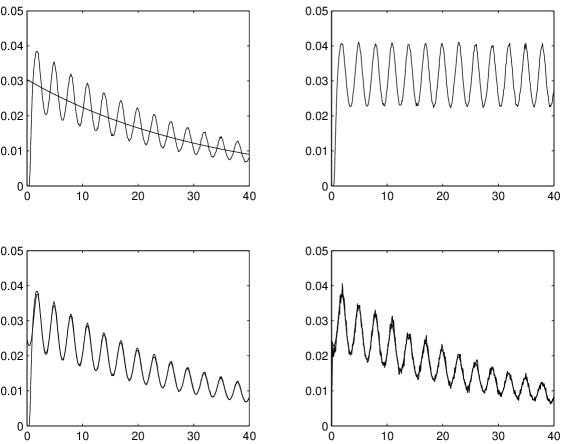
Figure 2: For a zero-mean stationary Gaussian process with covariance (5) and $\alpha=\beta=1$ in the presence of the periodic boundary $S(t)=2+0.1\,\sin(2\,\pi\,t/3),$ the simulated FPT density ${\tilde{g}}(t)$ is compared with the exponential density ${\widehat{\lambda}}\,e^{-{\widehat{\lambda}}\,t}$, with ${\widehat{\lambda}}=0.030386$ in (a). The function ${\tilde{Z}}(t)=\tilde{g}(t)\,\exp\bigl{\{}{{\widehat{\lambda}}\,t}\bigr{\}}$ is plotted in (b). The asymptotic exponential approximation is plotted together with the simulated FPT density $\tilde{g}(t)$ in (c). The asymptotic exponential approximation is plotted together with the simulated upcrossing FPT density $\tilde{g}_{u}(t)$ in (d).

3 Asymptotic results

The asymptotic behavior of the FPT densities for Gaussian processes as boundaries or time grow larger has been studied in [9], [10] and [11]. Our analysis is a natural extension of some investigations performed for the Ornstein-Uhlenbeck (OU) process [18] and successively extended to the class of one-dimensional diffusion processes admitting steady state densities in the presence of single asymptotically constant boundaries or of single asymptotically periodic boundaries (see [14] and [17]). There, computational as well as analytical results have indicated that the conditioned FPT pdf is susceptible of an excellent non-homogeneous exponential approximation for large boundaries, even though these boundaries need not be very distant from the initial state of the process. To this aim, we have estimated such a density by generating the sample paths of the Gaussian process through the parallel simulation algorithm implemented on the super-computer CRAY T3E of CINECA in order to overcome the outrageous complexity offered by the numerical evaluation of the involved partial sums of the conditioned FPT pdf series expansion. Specifically, we have considered the class of zero-mean stationary Gaussian processes characterized by damped oscillatory covariances (see [9]):

$$\gamma(t)=e^{-\beta\,|t|}\,\Bigl{[}\cos\bigl{(}\alpha\,t)+\,\sin\bigl{(}\alpha|t|)\Bigr{]},$$ (5)

where $\alpha$ and $\beta$ are positive real numbers.

The results of our computations have shown that for certain periodic boundaries of the form

$$S(t)=S_{0}+A\,\sin\bigl{(}2\,\pi\,t/Q\bigr{)},\quad S_{0},A,Q>0,$$ (6)

not very distant from the initial value of the process, the FPT pdf soon exhibits damped oscillations having the same period of the boundary. Furthermore, starting from rather small times, the estimated FPT densities $\tilde{g}(t)$ appears to be representable in the form

$$\tilde{g}(t)\simeq\tilde{Z}(t)\;e^{-\widehat{\lambda}\,t},$$ (7)

where $\widehat{\lambda}$ is a constant that can be estimated by the least squares methods, and where $\tilde{Z}(t)$ is a periodic boundary of period $T$ (see, for example, Figure 2(a) and Figure 2(b)). The goodness of the exponential approximation increases as the boundary is progressively moved farther apart from the starting point of the process. The more the periodic boundary is far from the starting point of the process, the more the exponential approximation improves.

In [11] we have shown by rigorous mathematical arguments that as boundary (6) moves away from the initial state of the process, the FPT pdf approaches a non-homogeneous exponential density of the type

$$\tilde{g}(t)\sim\tilde{h}(t)\exp\left\{-\int_{0}^{t}\tilde{h}(\tau)d\tau\right\},$$ (8)

where

$$\tilde{h}(t)={\sqrt{\alpha^{2}+\beta^{2}}\over 2\,\pi}\exp\biggl{\{}-{S^{2}(t)\over 2}\biggr{\}}\,\biggl{[}\exp\biggl{\{}-{[\dot{\rho}(t)]^{2}\over 2\,(\alpha^{2}+\beta^{2})}\biggr{\}}$$

$$\hskip 113.81102pt-\sqrt{{\pi\over 2\,(\alpha^{2}+\beta^{2})}}\,\dot{\rho}(t)\,{\rm Erfc}\,\biggl{(}{\dot{\rho}(t)\over\sqrt{2\,(\alpha^{2}+\beta^{2})}}\biggr{)}\biggr{]}$$ (9)

and $\rho(t)=A\sin(2\pi t/Q).$ (See, for example, Figure 2(c)). In [10] a similar result is proved for the upcrossing FPT density. (See Figure 2(d)).

Figure 3: For different choices of $\vartheta$ in the interval $[0.008,1.024]$, with threshold $S(t)=-t^{2}/2-t+5$, plot of the simulated $\tilde{g}_{u}(t)$ is shown in (a) and plot of $\tilde{g}_{u}(t)$ for the OU-model in (c). Same in (b) and (d) for values of $\vartheta$ in $[2.048,200].$

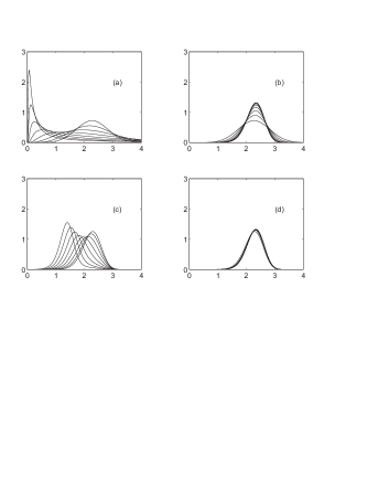
Figure 4: For different choices of $\vartheta$ in the interval $[0.008,1.024]$, with the same boundary as in Figure 3, plot of $\tilde{g}_{u}(t)$ for the Wiener model is shown in (a) and plot of $q(t)$ for the Kostyukov-model in (c). Same in (b) and (d) for values of $\vartheta$ in $[2.048,200].$

It should be stressed that the analytic and the simulation results constitutes only a preliminary step towards the construction of neuronal models based on non-Markov processes. Nevertheless, the unveiling of properties of the asymptotic behavior of FPT may turn out to be useful also for the description of neuronal activities at small times whenever the intrinsic time scale of the microscopic events involved during the neuron’s evolution is much smaller than the macroscopic observation time scale, or when the asymptotic regime is exhibited also in the case of firing thresholds not too distant from the resting potential, similarly to what was already pointed out by us in connection with the OU neuronal model [14].

4 An alternative approach

Within the context of single neuron’s activity modeling a completely different, apparently not well known, approach was proposed by Kostyukov et al. ([16]) in which a non-Markov process of a Gaussian type is assumed to describe the time course of the neural membrane potential. The model due to Kostyukov (K-model) makes use of the notion of correlation time. Namely, let $X(t)$ be a stationary Gaussian process with zero mean, unit variance and correlation function $R(t)$. Then [21],

$$\vartheta=\int_{0}^{+\infty}|R(\tau)|\;d\tau<+\infty$$

is defined as the correlation time of the process $X(t).$ Under some assumptions on the threshold and by using a sort of diffusion approximation, Kostyukov works out a numerical evaluation $q(t)$ to the upcrossing FPT pdf. This approximation is obtained as solution of an integral equation that can be solved by routine methods. The relevant feature of this approach is that the unique parameter $\vartheta$ characterizes the considered class of stationary standard Gaussian processes.

In [2] and in [5] we analyzed this method pinpointing similarities and differences with respect to our models. Recently [12], we have again made use of the K-model and compared the obtained results with those worked out by numerically solving the integral equation holding for Gauss-Markov processes in the case of the OU and Wiener models, see [5] for details, and with the results obtained via the simulations of Gaussian processes. A variety of thresholds and of $\vartheta$ values has been considered. For some values of $\vartheta$ between 0.008 and 200, our results have been plotted in Figures 3 and 4.

Our investigations in this direction suggest that the validity of approximations of the firing densities in the presence of memory effects by the FPT densities of Markov type is clearly depending on the magnitude of the correlation time. Hence, an object of our present research is the investigation of those models whose asymptotic behavior becomes increasingly similar as the correlation time $\vartheta$ grows larger.

References

- [1] A. Buonocore, A.G. Nobile and L.M. Ricciardi, A new integral equation for the evaluation of first-passage-time probability densities. Adv. Appl. Prob. 19, 784–800 (1987).
- [2] A. Di Crescenzo, E. Di Nardo, A.G. Nobile, E. Pirozzi and L.M. Ricciardi, On some computational results for single neurons’ activity modeling. BioSystems 58, 19–26 (2000).
- [3] E. Di Nardo, E. Pirozzi, L.M. Ricciardi and S. Rinaldi, Vectorized simulations of normal processes for first crossing-time problems. Lecture Notes in Computer Science 1333, 177–188 (1997).
- [4] E. Di Nardo, A.G. Nobile, E. Pirozzi, L.M. Ricciardi and S. Rinaldi, Simulation of Gaussian processes and first passage time densities evaluation. Lecture Notes in Computer Science 1798, 319-333 (2000).
- [5] E. Di Nardo, A.G. Nobile, E. Pirozzi and L.M. Ricciardi, On a non-Markov neuronal model and its approximation. BioSystems 48, 29–35 (1998).
- [6] E. Di Nardo, A.G. Nobile, E. Pirozzi and L.M. Ricciardi, Evaluation of upcrossing first passage time densities for Gaussian processes via a simulation procedure. Atti della Conferenza Annuale della Italian Society for Computer Simulation. 95-102 (1999).
- [7] E. Di Nardo, A.G. Nobile, E. Pirozzi and L.M. Ricciardi, Parallel simulations in FPT problems for Gaussian processes. Science and Supercomputing at CINECA. Report 2001, 405–412 (2001).
- [8] E. Di Nardo, A.G. Nobile, E. Pirozzi and L.M. Ricciardi, A computational approach to first-passage-time problem for Gauss-Markov processes. Adv. Appl. Prob. 33, 453–482 (2001).
- [9] E. Di Nardo, A.G. Nobile, E. Pirozzi and L.M. Ricciardi, Computer-aided simulations of Gaussian processes and related asymptotic properties. Lecture Notes in Computer Science, 2178, 67–78 (2001).
- [10] E. Di Nardo, A.G. Nobile, E. Pirozzi and L.M. Ricciardi, Gaussian processes and neuronal models: an asymptotic analysis. Cybernetics and Systems 2, 313–318 (2002).
- [11] E. Di Nardo, A.G. Nobile, E. Pirozzi and L.M. Ricciardi, On the asymptotic behavior of first passage time densities for stationary Gaussian processes and varying boundaries. Methodology and Computing in Applied Probability, 5, 211-233, (2003).
- [12] E. Di Nardo, A.G. Nobile, E. Pirozzi and L.M. Ricciardi, Computational Methods for the evaluation of Neuron’s Firing Densities. Lecture Notes in Computer Science, 2809, 394-403 (2003).
- [13] E. Di Nardo, A.G. Nobile, E. Pirozzi and L.M. Ricciardi, Towards the Modeling of Neuronal Firing by Gaussian Processes. Scientiae Mathematicae Japonicae 58, No. 2, 255-264 (e8, 497-506), (2003).
- [14] V. Giorno, A.G. Nobile and L.M. Ricciardi, On the asymptotic behavior of first-passage-time densities for one-dimensional diffusion processes and varying boundaries. Adv. Appl. Prob. 22, 883–914 (1990).
- [15] J.N. Franklin, Numerical simulation of stationary and non stationary gaussian random processes. SIAM Review 7, 68–80 (1965).
- [16] A. I. Kostyukov, Yu.N. Ivanov and M.V. Kryzhanovsky, Probability of Neuronal Spike Initiation as a Curve-Crossing Problem for Gaussian Stochastic Processes. Biological Cybernetics. 39, 157-163 (1981).
- [17] A.G. Nobile, L.M. Ricciardi and L. Sacerdote, Exponential trends of Ornstein-Uhlenbeck first passage time densities. J. Appl. Prob. 22 360–369 (1985).
- [18] A.G. Nobile, L.M. Ricciardi and L. Sacerdote, Exponential trends of first-passage-time densities for a class of diffusion processes with steady-state distribution. J. Appl. Prob. 22 611–618 (1985).
- [19] L.M. Ricciardi and S. Sato, On the evaluation of first-passage-time densities for Gaussian processes. Signal Processing. 11 339-357 (1986).
- [20] L.M. Ricciardi, Diffusion Processes and Related Topics in Biology. Springer-Verlag, New York, (1977).
- [21] R.L. Stratonovich, Topics in Theory of Random Noise. Vol. 1, Gordon and Breach, New York, (1963).
- [22] A.M. Yaglom, Correlation Theory of Stationary Related Random Functions. Vol. I: Basic Results. Springer-Verlag, New York, (1987).