Abstract

We study initial boundary value problems for linear scalar evolution partial differential equations, with spatial derivatives of arbitrary order, posed on the domain $\{t>0,\;0<x<L\}$. We show that the solution can be expressed as an integral in the complex $k$-plane. This integral is defined in terms of an $x$-transform of the initial condition and a $t$-transform of the boundary conditions. The derivation of this integral representation relies on the analysis of the global relation, which is an algebraic relation defined in the complex $k$-plane coupling all boundary values of the solution.

For particular cases, such as the case of periodic boundary conditions, or the case of boundary value problems for even order PDEs, it is possible to obtain directly from the global relation an alternative representation for the solution, in the form of an infinite series. We stress however that there exist initial boundary value problems for which the only representation is an integral which cannot be written as an infinite series. An example of such a problem is provided by the linearised version of the KdV equation. Similarly, in general the solution of odd-order linear initial boundary value problems on a finite interval cannot be expressed in terms of an infinite series.

Keywords: boundary value problems, evolution PDEs, generalised Fourier transforms, spectral transforms

1 Introduction

An evolution partial differential equation in one space dimension is characterised by its symbol, which we denote by $\omega(k)$. This means that a particular solution of the equation is given by

$$E_{k}(x,t)={\rm e}^{ikx-\omega(k)t},\quad{\rm any}\;k\in\,\mathbb{C}.$$

Physically significant examples of scalar evolution equations are:

(a) the Schrödinger equation with zero potential

$$iq_{t}+q_{xx}=0,\quad\omega(k)=ik^{2};$$ (1.1)

(b) the heat equation

$$q_{t}-q_{xx}=0,\quad\omega(k)=k^{2};$$ (1.2)

(c) the Stokes equation

$$q_{t}+q_{xxx}+q_{x}=0,\quad\omega(k)=i(k-k^{3}).$$ (1.3)

We note that equations (1.1) and (1.3) are the linearised versions of the nonlinear Schrödinger and of the Korteweg-deVries equations respectively.

Notations

The following notations, used throughout the paper, refer to a linear evolution PDE of order $n$, whose symbol $\omega(k)$ is assumed to be a polynomial of degree $n$.

• $q_{0}(x)$ denotes the given initial condition, and $\hat{q}_{0}(k)$ the Fourier transform of $q_{0}(x)$:

  $$q_{0}(x)=q(x,0),\;\;0<x<L;\;\;\;\hat{q}_{0}(k)=\int_{0}^{L}q_{0}(x){\rm e}^{-ikx}dx,\;\;k\in{\mathbb{C}}.$$ (1.4)

• $\{f_{j}(t)\}_{0}^{n-1}$ and $\{g_{j}(t)\}_{0}^{n-1}$ denote the boundary values of the solution at $x=0$ and $x=L$ respectively, while $\{\tilde{f}_{j}(t,k)\}_{0}^{n-1}$ and $\{\tilde{g}_{j}(t,k)\}_{0}^{n-1}$ denote certain $t$-transforms of $f_{j}$ and $g_{j}$:

  $$f_{j}(t)=\partial_{x}^{j}q(0,t),\;\;t>0;\;\;\;\tilde{f}_{j}(t,k)=\int_{0}^{t}{\rm e}^{\omega(k)s}f_{j}(s)ds,\;\;k\in{\mathbb{C}},\;t>0,$$ (1.5)

  $$g_{j}(t)=\partial_{x}^{j}q(L,t),\;\;t>0;\;\;\;\tilde{g}_{j}(t,k)=\int_{0}^{t}{\rm e}^{\omega(k)s}g_{j}(s)ds,\;\;k\in{\mathbb{C}},\;t>0,$$ (1.6)

  where $j=0,\ldots,n-1$.

• The domain $D$ in the complex $k$-plane is defined by

  $$D=\{k\in{\mathbb{C}}:\;{\rm Re}\,\omega(k)\leq 0\}.$$ (1.7)

  $D^{+}$ and $D^{-}$ denote the part of $D$ in the upper and lower half of the complex $k$-plane respectively:

  $$D^{+}=\{k\in{\mathbb{C}}:k\in\,D,\;{\rm Im}(k)\geq 0\},\quad D^{-}=\{k\in{\mathbb{C}}:k\in\,D,\;{\rm Im}(k)\leq 0\}.$$ (1.8)

  The oriented boundaries of $D^{+}$ and $D^{-}$ are denoted by $\partial D^{+}$ and $\partial D^{-}$, where the orientation is such that the interior of the domain $D$ is always on the left of the positive direction.

Statement of the problem and assumptions

Let $q(x,t)$ satisfy a linear evolution equation with symbol $\omega(k)$ in the domain

$$\left\{t>0,\quad 0<x<L\right\},$$

where $L$ is a finite positive constant. We assume that $\omega(k)$ is a polynomial of degree $n$ such that the equation $\omega(k)=0$ has $n$ distinct roots, and that Re $\omega(k)\geq 0$ for $k\in\,{\mathbb{R}}$. We assume that the initial condition $q_{0}(x)$ is a given, sufficiently smooth, function.

We consider the two following questions:

(i) Determine the number of boundary conditions that must be prescribed at $x=0$ and $x=L$ in order to define a well posed problem.

(ii) Given appropriate boundary conditions at the two ends of the space interval, and assuming that these given functions have sufficient smoothness and are compatible with $q_{0}(x)$ at $x=0$ and $x=L$, construct the solution $q(x,t)$.

Problem (i) was solved in [8, 10], where it was shown that the number of boundary conditions that must be prescribed for a well posed problem are $N$ at $x=0$ and $n-N$ at $x=L$, where

$$N=\left\{\begin{array}[]{ll}n/2&n\;\;{\rm even},\\ (n+1)/2&n\;\;{\rm odd},\;\;c_{n}>0,\\ (n-1)/2&n\;\;{\rm odd},\;\;c_{n}<0,\end{array}\right.$$ (1.9)

where $c_{n}$ is the coefficient of $k^{n}$ in the symbol $\omega(k)$. We explain in appendix A the motivation for this choice of $N$.

In this paper we address question (ii).

The new method

The new method used here to analyse boundary value problems for equations with spatial derivatives of arbitrary order $n$ is mathematically straightforward, yet it yields results which are difficult to obtain by the standard approaches. This method, which is the implementation to this class of problems of the general approach introduced by one of the authors [4], involves the steps outlined below.

(a) Reformulation of the PDE

A given evolution PDE with symbol $\omega(k)$ can be written in the form

$$\left({\rm e}^{-ikx+\omega(k)t}q\right)_{t}-\left({\rm e}^{-ikx+\omega(k)t}X\right)_{x}=0,\quad k\in{\mathbb{C}},$$ (1.10)

where $q(x,t)$ is a solution of the PDE, and the function $X(x,t,k)$ is given by the formula

$$X(x,t,k)=\sum_{j=0}^{n-1}c_{j}(k)\partial_{x}^{j}q(x,t),$$ (1.11)

where the coefficients $c_{j}(k)$ are known polynomials in $k$. For example, for equation (1.1), $n=2$, $c_{1}(k)=-k$ and $c_{2}(k)=i$. The explicit form of $c_{j}(k)$ for an arbitrary $\omega(k)$ is given in section 2.

Equation (1.10) is in the form

$$\frac{\partial P}{\partial t}-\frac{\partial Q}{\partial x}=0,$$

with

$$P(x,t)={\rm e}^{-ikx+\omega(k)t}q(x,t),\quad Q(x,t)={\rm e}^{-ikx+\omega(k)t}X(x,t,k).$$

Green’s theorem applied to the domain ${\cal D}=\{[0,L]\times[0,t]\}$ yields

$$\int\int_{\cal D}\left(\frac{\partial P}{\partial t}-\frac{\partial Q}{\partial x}\right)dxdt=\int_{\partial\cal D}Qdt+Pdx,$$

thus

$$\int_{\partial\cal D}Qdt+Pdx=0.$$

Substituting in the latter expression the explicit definition of $P$ and $Q$, with $X(x,t,k)$ given by (1.11), we obtain the global relation

$$\sum_{0}^{n-1}c_{j}(k)\left(\tilde{f}_{j}(t,k)-{\rm e}^{-ikL}\tilde{g}_{j}(t,k)\right)=\hat{q}_{0}(k)-{\rm e}^{\omega(k)t}\hat{q}(t,k),\quad k\in{\mathbb{C}},$$ (1.12)

where $\hat{q}_{0}$, $\tilde{f}_{j}$ and $\tilde{g}_{j}$ are defined in the notations (equations (1.4)-(1.6))and $\hat{q}(t,k)$ denotes the $x$-Fourier transform of $q(x,t)$.

Solving equation (1.12) with respect to $\hat{q}(t,k)$ and then taking the inverse Fourier transform of the resulting expression, we obtain the following formula for $q(x,t)$:

$$q(x,t) = \frac{1}{2\pi}\left\{\int_{-\infty}^{\infty}{\rm e}^{ikx-\omega(k)t}\hat{q}_{0}(k)dk-\int_{-\infty}^{\infty}{\rm e}^{ikx-\omega(k)t}\sum_{j=0}^{n-1}c_{j}(k)\tilde{f}_{j}(t,k)dk\right.$$ (1.13)

$$+ \left.\int_{-\infty}^{\infty}{\rm e}^{ik(x-L)-\omega(k)t}\sum_{j=0}^{n-1}c_{j}(k)\tilde{g}(t,k)dk\right\}.$$

We note however that this expression is not effective, since it contains the $t$-transforms of all the boundary values of the solution $q(x,t)$, while only a subset of these boundary values is prescribed as boundary conditions.

(b) The integral representation of the solution

Using the analyticity properties of the functions $\tilde{f}_{j}$ and $\tilde{g}_{j}$ and Cauchy’s theorem to deform the contour of integration, we show in section 4 that the expression (1.13) can be written as

$$q(x,t) = \frac{1}{2\pi}\left\{\int_{-\infty}^{\infty}{\rm e}^{ikx-\omega(k)t}\hat{q}_{0}(k)dk-\int_{\partial D^{+}}{\rm e}^{ikx-\omega(k)t}\sum_{j=0}^{n-1}c_{j}(k)\tilde{f}_{j}(t,k)dk\right.$$ (1.14)

$$- \left.\int_{\partial D^{-}}{\rm e}^{ik(x-L)-\omega(k)t}\sum_{j=0}^{n-1}c_{j}(k)\tilde{g}(t,k)dk\right\},$$

where $\partial D^{+}$, $\partial D^{-}$ are defined in the notations. The advantage of this form of the representation is that the $t$-transforms of all boundary values can now be computed explicitly. Indeed, it will be shown in section 4 that the functions $\tilde{f}_{j}$ and $\tilde{g}_{j}$, $j=0,\ldots,n-1$, for $k\in D^{\pm}$ respectively, can be expressed in terms of the given initial and boundary conditions. For example, it will be shown in that section that the solution of the boundary value problem   for equation (1.3) with the boundary conditions

$$q(0,t)=f_{0}(t),\quad q(L,t)=g_{0}(t),\quad q_{x}(L,t)=g_{1}(t),\quad t>0,$$ (1.15)

is given by equation (1.14), where the contours $\partial D^{+}$ and $\partial D^{-}$ are shown in figure 1, $\omega(k)=i(k-k^{3})$, $c_{0}=k^{2}-1$, $c_{1}=-ik$, $c_{2}=1$, $\tilde{f}_{0}$, $\tilde{g}_{0}$ and $\tilde{g}_{1}$ are defined in terms of $f_{0}$, $g_{0}$ and $g_{1}$ by equations (1.5) and (1.6), and the functions $\tilde{f}_{1}$, $\tilde{f}_{2}$ and $\tilde{g}_{2}$ are given in terms of the given initial and boundary conditions by the following expressions:

$$i\tilde{f}_{1} = \frac{1}{\Delta(k)}\left[{\rm e}^{-ikL}(N(\lambda_{2},t)-N(\lambda_{1},t))+{\rm e}^{-i\lambda_{1}L}(N(k,t)-N(\lambda_{2},t))+{\rm e}^{-i\lambda_{2}L}(N(\lambda_{1},t)-N(k,t))\right],$$

$$\tilde{f}_{2} = \frac{1}{\Delta(k)}\left[{\rm e}^{-ikL}(\lambda_{2}N(\lambda_{1},t)-\lambda_{1}N(\lambda_{2},t))+{\rm e}^{-i\lambda_{1}L}(kN(\lambda_{2},t)-\lambda_{2}N(k,t))\right.$$

$$\left.\hskip 30.0pt+{\rm e}^{-i\lambda_{2}L}(\lambda_{1}N(k,t)-kN(\lambda_{1},t))\right],$$

$$\tilde{g}_{2} = \frac{1}{\Delta(k)}\left[(N(k,t)(\lambda_{2}-\lambda_{1})+N(\lambda_{1},t)(\lambda_{2}-k)+N(\lambda_{2},t))(k-\lambda_{1})\right],$$ (1.16)

where $\Delta(k)$ and $N(k)$ are defined by

$$\Delta(k)={\rm e}^{-ikL}(\lambda_{1}-\lambda_{2})+{\rm e}^{-i\lambda_{2}L}(k-\lambda_{1})+{\rm e}^{-i\lambda_{1}L}(\lambda_{2}-k),$$ (1.17)

$$N(k,t)=(1-k^{2})(\tilde{f}_{0}(t,k)-{\rm e}^{-ikL}\tilde{g}_{0}(t,k))-ik{\rm e}^{-ikL}\tilde{g}_{1}(t,k)+\hat{q}_{0}(k),$$ (1.18)

and $\lambda_{1}(k)$, $\lambda_{2}(k)$ are the two roots of the polynomial $\lambda^{2}+\lambda k+k^{2}-1=0$.

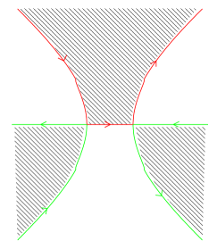
Figure 1: The domain $D$ and the contours $\partial D^{+}$ (in red) and $\partial D^{-}$ (in green) for equation (1.3). Note that $D^{-}$ has two connected components.

(c) The global relation and its analysis

Although the derivation of the global relation (1.12) is elementary, this equation plays a central role in the analysis. The crucial observation is that the functions $\tilde{f}_{j}$ and $\tilde{g}_{j}$ depend on $k$ only through $\omega(k)$. Thus these functions are invariant under any transformation of the complex $k$-plane that leaves $\omega(k)$ invariant. These transformations are determined by the roots of the equation $\omega(k)=\omega(\lambda)$. These roots are by our assumption distinct, and are given by

$$\lambda_{0}(k)=k,\lambda_{1},\ldots,\lambda_{n-1}.$$ (1.19)

Replacing $k$ by $\lambda(k)$ in equation (1.12) we obtain a system of $n$ equations

$$\sum_{j=0}^{n-1}c_{j}(\lambda_{l}(k))\left(\tilde{f}_{j}(t,k)-{\rm e}^{-i\lambda_{l}(k)L}\tilde{g}_{j}(t,k)\right)=\hat{q}_{0}(\lambda_{l}(k))-{\rm e}^{\omega(k)t}\hat{q}(t,\lambda_{l}(k)),\quad l=0,..,n-1.$$ (1.20)

Ignoring for the moment the unknown function $\hat{q}(t,k)$, equations (1.20) can be considered as $n$ equations coupling the $2n$ unknown functions $\{\tilde{f}_{j},\tilde{g}_{j}\}_{0}^{n-1}$; $n$ of these functions can be computed immediately, and the remaining $n$ unknown functions can be obtained by solving this system of $n$ equations.

More specifically, let $f_{p}(t)$ and $g_{r}(t)$ denote the prescribed boundary conditions, where $p$ and $r$ take $N$ and $n-N$ integer values respectively. Then $\tilde{f}_{p}$ and $\tilde{g}_{r}$ can be computed immediately (see equations (1.5) and (1.6)). Let $f_{P}(t)$ and $g_{R}(t)$ denote the remaining unknown boundary values. Solving the $n$ algebraic equation (1.20) for $\tilde{f}_{P}$ and $\tilde{g}_{R}$ it follows that these unknown functions can be expressed in terms of $\hat{q}_{0}$, $\{\tilde{f}_{p},\tilde{g}_{r}\}$, and of a term involving $\hat{q}(t,\lambda(k))$ and $1/\Delta(k)$, where $\Delta(k)$ denotes the determinant of the relevant system. It was shown in [8, 10] that in order for the terms involving the unknown functions $\hat{q}(t,\lambda_{j}(k))$ not to contribute to $q(x,t)$, $N$ must be chosen by equation (1.9). Indeed, in this case, the terms involving $\hat{q}(t,\lambda(k))$ appearing in the representation of $\tilde{f}_{P}$ are bounded as $k\to\infty$, $k\in\,D^{+}$. Therefore, if $\Delta(k)\neq 0$, $k\in\,D^{+}$, using Cauchy theorem in the domain $D^{+}$, it follows that these expressions give a zero contribution. If $\Delta(k)=0$, for infinitely many $k\in\,D^{+}$, it can be shown that these zeros must be on $\partial D^{+}$ [11]. In this case, the contour deformation from $\mathbb{R}$ to $\partial D^{+}$ must avoid these zeros. The integral representation is then obtained along the indented contour, and as in the previous case the terms involving $\hat{q}(t,\lambda(k))$ give a zero contribution.

The analysis of the terms $\tilde{g}_{R}$ is similar.

Thus even if $\Delta(k)$ has zeros in $D$, these zeros can be avoided by a contour indentation, and an integral representation of $q(x,t)$ can always be constructed. The determination of the zeros of $\Delta(k)$ becomes increasingly more complicated as the order $n$ of the equation grows. However, $\Delta(k)$ is always an analytic function of finite order, in the form of a finite exponential sum (the order of an entire function is a measure of its rate of growth as $k\to\infty$). For such entire functions there exists an extensive theory, implying in particular that such a function has infinitely many zeros accumulating at infinity, which lie along specific rays in the complex plane, see [9]. A brief overview of the relevant theory is given in Appendix B. This knowledge is sufficient to determine when these zeros are inside or outside the domain $D$.

(d) The series representation

For even order problems, separation of variables gives rise to a self-adjoint $x$-differential operator, which in this case can be used to construct the solution in the form of a series. For odd order problems, the associated $x$-operator is not, in general, self-adjoint. For particular boundary conditions (which do not include the uncoupled boundary conditions arising in many applications), it is possible to construct a self-adjoint extension, and thus for these particualr boundary value problems it is also possible to obtain the solution in the form of a series.

There exist the following alternative, simple way to construct these series representations: evaluate equations (1.20) at the zeros of $\Delta(k)$. We note that this evaluation is possible only if all the terms appearing in equations (1.20) are bounded at these zeros. In this respect we differentiate between the even and odd order problems: for even order problems, this evaluation is always possible, independently of whether the zeros of $\Delta(k)$ are inside or outside of the domain $D$. However, for odd order problems, it turns out that this evaluation is possible only if the zeros of $\Delta(k)$ are in $D$ (corresponding to the case of odd order problems for which there exists a self-adjoitn extension). For typical boundary value problems , with uncoupled boundary conditions, the zeros of $\Delta(k)$ are outside $D$, and thus it is not possible to obtain a series representation (1.14).

Consider for example equation (1.1) and assume for simplicity that homogeneous Dirichlet boundary conditions are prescribed. Then $\tilde{f}_{0}=\tilde{g}_{0}=0$ and $\lambda_{1}=-k$, hence equations (1.20) become

$$i\tilde{f}_{1}-i{\rm e}^{-ikL}\tilde{g}_{1} = \hat{q}_{0}(k)-{\rm e}^{ik^{2}t}\hat{q}(t,k),$$

$$i\tilde{f}_{1}-i{\rm e}^{ikL}\tilde{g}_{1} = \hat{q}_{0}(-k)-{\rm e}^{ik^{2}t}\hat{q}(t,-k).$$

Subtracting these equations we obtain

$$i({\rm e}^{ikL}-{\rm e}^{-ikL})\tilde{g}_{1}=\hat{q}_{0}(k)-\hat{q}_{0}(-k)-{\rm e}^{ik^{2}t}\left(\hat{q}(t,k)-\hat{q}(t,-k)\right).$$

Evaluating this equation at the values of $k$ for which the coefficient of $\tilde{g}_{1}$ vanishes, i.e. $k=k_{m}:=\frac{m\pi}{L}$, $m\in{\mathbb{Z}}$, and using the definition of $\hat{q}_{0}(k)$ and $\hat{q}(t,k)$ we find

$$\hat{q}^{(sin)}(t,k_{m})={\rm e}^{-ik_{m}^{2}t}\hat{q}_{0}^{(sin)}(k_{m}),\quad\hat{q}^{(sin)}(k_{m})=\int_{0}^{L}\sin(k_{m}x)q(x)dx.$$ (1.21)

Equation (1.21a) can be inverted by the well known formula and then $q(x,t)$ is expressed in the form of a sine series. Equation (1.21) can also be obtained by the use of the $x$-sine transform, which is the appropriate $x$-transform for this problem.

The above computation relies on the fact that all terms involved in the global relation are bounded at the zeros of $\Delta(k)$. This is to be contrasted with the case of equation (1.3) with $q(0,t)=q(L,t)=q_{x}(L,t)=0$. In this case, letting $\tilde{f}_{0}=\tilde{g}_{0}=\tilde{g}_{1}=0$, and evaluating the global relation at $k$, $\lambda_{1}(k)$ and $\lambda_{2}(k)$, we obtain a system of three algebraic equations for $\tilde{f}_{1}$, $\tilde{f}_{2}$ and $\tilde{g}_{2}$. The determinant of this system vanishes at $k=k_{m}$, $m\in\,{\mathbb{Z}}$, where for large $k$, arg$(k_{m})$ is either $\pi/6$, $5\pi/6$ or $3\pi/2$, so that $k_{m}\notin D$. It can be verified that the functions $\tilde{f}_{1}$, $\tilde{f}_{2}$ and $\tilde{g}_{2}$ involve ${\rm e}^{i(k-k^{3})t}$, thus they become unbounded at $k=k_{m}$, $k\to\infty$. Hence, we cannot evaluate this system at the zeros of its determinant. A more detailed discussion is given in [11].

We note that when such a representation exists, it can also be obtained by using the explicit residue computation of the general integral representation.

2 The elements of the method

It can be verified (see [6]) that a PDE with symbol $\omega(k)$ can be written in the form

$$\left({\rm e}^{-ikx+\omega(k)t}q\right)_{t}-\left({\rm e}^{-ikx+\omega(k)t}X\right)_{x}=0,\quad k\in{\mathbb{C}},$$ (2.1)

where the function $X(x,t,k)$ is given by the formula

$$X(x,t,k)=i\frac{\omega(k)-\omega(-i\partial_{x})}{k+i\partial_{x}}q(x,t).$$ (2.2)

In what follows we give the function $X$, the domains $D^{+}$, $D^{-}$, and equations (1.20) for equations (1.1)-(1.3).

(a) The equation (1.1)

The symbol is

$$\omega(k)=ik^{2}.$$

Indeed, ${\rm e}^{ikx-ik^{2}t}$ satisfies this equation. In this case

$${\rm Re}\,\omega(k)={\rm Re}(ik^{2})=-2{\rm Re}(k){\rm Im}(k).$$

Thus the domain $D$ is the union of the first and third quadrants of the $k$ complex plane:

$$D=\{k\in{\mathbb{C}}^{+}:{\rm Re}(k){\rm Im}(k)\geq 0\}.$$ (2.3)

The equation $\omega(k)=\omega(\lambda)$ implies

$$\lambda^{2}-k^{2}=(\lambda-k)(\lambda+k)=0$$

hence $\lambda_{1}(k)=-k$. Equation (1.11) yields

$$X(x,t,k)=i\frac{ik^{2}+i\partial_{x}^{2}}{k+i\partial_{x}}q=-\frac{(k+i\partial_{x})(k-i\partial_{x})}{k+i\partial_{x}}q=iq_{x}-kq.$$

The PDE (1.1) is thus equivalent to the expression

$$\left({\rm e}^{-ikx+ik^{2}t}q\right)_{t}-\left({\rm e}^{-ikx+ik^{2}t}(iq_{x}-kq)\right)_{x}=0,\quad k\in{\mathbb{C}}.$$ (2.4)

The global relation is

$$i\tilde{f}_{1}(t,k)-k\tilde{f}_{0}(t,k)-{\rm e}^{-ikL}\left(i\tilde{g}_{1}(t,k)-k\tilde{g}_{0}(t,k)\right)=\hat{q}_{0}(k)-{\rm e}^{ik^{2}t}\hat{q}(t,k).$$ (2.5)

Since $\lambda_{1}=-k$, we supplement this equation with the equation

$$i\tilde{f}_{1}(t,k)+k\tilde{f}_{0}(t,k)-{\rm e}^{ikL}\left(i\tilde{g}_{1}(t,k)+k\tilde{g}_{0}(t,k)\right)=\hat{q}_{0}(-k)-{\rm e}^{ik^{2}t}\hat{q}(t,-k).$$ (2.6)

(b) The equation (1.2)

The symbol is

$$\omega(k)=k^{2}.$$

The domain $D$ is in this case given by

$$D=\{k\in{\mathbb{C}}:\;\pi/4\leq{\rm arg}\,(k)\leq 3\pi/4\;\;{\rm or}\;\;5\pi/4\leq{\rm arg}\,(k)\leq 7\pi/4\}.$$ (2.7)

and $D^{\pm}=D\cap{\mathbb{C}}^{\pm}$, see figure 2.

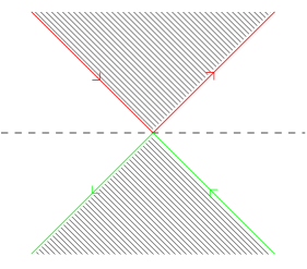
Figure 2: The domain $D$ and the contours $\partial D^{+}$ (in red) and $\partial D^{-}$ (in green) for equation (1.2)

The equation $\omega(k)=\omega(\lambda)$ implies, as for example (a), that $\lambda_{1}(k)=-k$. Equation (1.11) yields

$$X(x,t,k)=i\frac{k^{2}+\partial_{x}^{2}}{k+i\partial_{x}}q=i\frac{(k+i\partial_{x})(k-i\partial_{x})}{k+i\partial_{x}}q=ikq+q_{x}.$$ (2.8)

The PDE (1.2) is thus equivalent to the expression

$$\left({\rm e}^{-ikx+k^{2}t}q\right)_{t}-\left({\rm e}^{-ikx+k^{2}t}(ikq+q_{x})\right)_{x}=0,\quad k\in{\mathbb{C}}.$$ (2.9)

The global relation is

$$ik\tilde{f}_{0}(t,k)+\tilde{f}_{1}(t,k)-{\rm e}^{-ikL}\left(ik\tilde{g}_{0}(t,k)+\tilde{g}_{1}(t,k)\right)=\hat{q}_{0}(k)-{\rm e}^{k^{2}t}\hat{q}(t,k).$$ (2.10)

Since $\lambda_{1}=-k$, we supplement this equation with the equation

$$-ik\tilde{f}_{0}(t,k)+\tilde{f}_{1}(t,k)-{\rm e}^{ikL}\left(-ik\tilde{g}_{0}(t,k)+\tilde{g}_{1}(t,k)\right)=\hat{q}_{0}(-k)-{\rm e}^{k^{2}t}\hat{q}(t,-k).$$ (2.11)

(c) The equation (1.3)

The symbol is

$$\omega(k)=i(k-k^{3}).$$

The domain $D$ is in this case

$$D=\{k\in\,{\mathbb{C}}:\,{\rm Im}\,(k)\left[3{\rm Re}\,(k)^{2}-{\rm Im}\,(k)^{2}-1\right]\leq 0\},$$ (2.12)

see figure 1.

The equation $\omega(k)=\omega(\lambda)$ implies

$$(\lambda-\lambda^{3})-(k-k^{3})=(k-\lambda)(\lambda^{2}+\lambda k+k^{2}-1)=0,$$

hence

$$\lambda_{1}=\frac{\sqrt{4-3k^{2}}}{2}-\frac{k}{2},\quad\lambda_{2}=-\frac{\sqrt{4-3k^{2}}}{2}-\frac{k}{2}.$$

Equation (1.11) yields

$$X(x,t,k) = i\frac{i(k-k^{3})-(\partial_{x}+\partial_{x}^{3})}{k+i\partial_{x}}q=-\frac{(k+i\partial_{x}-k^{3}-i\partial_{x}^{3})}{k+i\partial_{x}}q$$ (2.13)

$$= \left\{-1+\frac{(k+i\partial_{x})(k^{2}-\partial_{x}^{2}-ik\partial_{x})}{k+i\partial_{x}}\right\}q=(k^{2}-1)q-ikq_{x}-q_{xx}.$$

The PDE (1.3) is thus equivalent to the expression

$$\left({\rm e}^{-ikx+i(k-k^{3})t}q\right)_{t}-\left({\rm e}^{-ikx+i(k-k^{3})t}((k^{2}-1)q-ikq_{x}-q_{xx})\right)_{x}=0,\quad k\in{\mathbb{C}}.$$ (2.14)

The global relation is

$$\left[(k^{2}-1)\tilde{f}_{0}-ik\tilde{f}_{1}-\tilde{f}_{2}\right]-{\rm e}^{-ikL}\left[(k^{2}-1)\tilde{g}_{0}-ik\tilde{g}_{1}-\tilde{g}_{2}\right]=\hat{q}_{0}(k)-{\rm e}^{i(k-k^{3})t}\hat{q}(t,k).$$ (2.15)

Supplementing this equation with the equations obtained from it by replacing $k$ with $\lambda_{1}$ and $\lambda_{2}$, we obtain

$$\left[(\lambda_{1}^{2}-1)\tilde{f}_{0}-i\lambda_{1}\tilde{f}_{1}-\tilde{f}_{2}\right]-{\rm e}^{-i\lambda_{1}L}\left[(\lambda_{1}^{2}-1)\tilde{g}_{0}-i\lambda_{1}\tilde{g}_{1}-\tilde{g}_{2}\right] = \hat{q}_{0}(\lambda_{1})-{\rm e}^{i(k-k^{3})t}\hat{q}(\lambda_{1},t),$$

$$\left[(\lambda_{2}^{2}-1)\tilde{f}_{0}-i\lambda_{2}\tilde{f}_{1}-\tilde{f}_{2}\right]-{\rm e}^{-i\lambda_{2}L}\left[(\lambda_{2}^{2}-1)\tilde{g}_{0}-i\lambda_{2}\tilde{g}_{1}-\tilde{g}_{2}\right] = \hat{q}_{0}(\lambda_{2})-{\rm e}^{i(k-k^{3})t}\hat{q}(\lambda_{2},t).$$

3 The zeros of $\Delta(k)$

We start by making the following general observations, valid for an arbitrary $\omega(k)$:

(i) The functions $\hat{q}_{0}(k)$ and $\hat{q}(t,k)$, which are entire functions of $k$, are bounded as $k\to\infty$ in ${\mathbb{C}}^{-}$, the lower half of the complex $k$-plane.

(ii) The functions ${\rm e}^{ikL}\hat{q}_{0}(k)$ and ${\rm e}^{ikL}\hat{q}(t,k)$ are bounded as $k\to\infty$ in ${\mathbb{C}}^{+}$, the upper half of the complex $k$-plane.

(iii) The functions $\tilde{f}_{j}$ and $\tilde{g}_{j}$, which are entire functions of $k$, are bounded as $k\to\infty$ if Re $\omega(k)\leq 0$.

Example (a)

Since $n=2$ and $N=1$, one boundary condition must be prescribed at each end. We consider equations (2.5)-(2.6) as two equations relating the four terms $\tilde{f}_{0}$, $\tilde{f}_{1}$, $\tilde{g}_{0}$, $\tilde{g}_{1}$, treating for the moment the function $\hat{q}(t,k)$ as a known function. If one of the functions $f_{j}$’s and one of the $g_{j}$’s are given, then the determinant of the system is of the form $\Delta(k)={\rm e}^{ikL}\pm{\rm e}^{-ikL}$. Hence its zeros are real, and given by either $k_{m}=m\pi/L$ or $k_{m}=(2m+1)\pi/2L$. Evaluating the solution of system (2.5)-(2.6) at these zeros yields the series representation of the solution for any such boundary value problem .

The Dirichlet problem

The given boundary conditions are

$$q(0,t)=f_{0}(t),\quad q(L,t)=g_{0}(t),\quad t>0.$$ (3.17)

Then $q(x,t)$ is given by

$$q(x,t)=\frac{i}{4L}\sum_{m}\sin(k_{m}x){\rm e}^{-ik_{m}^{2}t}\left[N(k_{m},t)-N(-k_{m},t)\right],\quad k_{m}=\frac{m\pi}{L},$$ (3.18)

where $N(k,t)$ is the known function

$$N(k,t)=k\left(\tilde{f}_{0}(t,k)-{\rm e}^{-ikL}\tilde{g}_{0}(t,k)\right)+\hat{q}_{0}(k).$$ (3.19)

Indeed, equations (2.5)-(2.6) yield

$$i\tilde{f}_{1}-{\rm e}^{-ikL}i\tilde{g}_{1} = N(k,t)-{\rm e}^{ik^{2}t}\hat{q}(t,k),$$

$$i\tilde{f}_{1}-{\rm e}^{ikL}i\tilde{g}_{1} = N(-k,t)-{\rm e}^{ik^{2}t}\hat{q}(t,-k).$$ (3.20)

Subtracting equations (3.20) we find

$$({\rm e}^{ikL}-{\rm e}^{-ikL})i\tilde{g}_{1}=N(k,t)-N(-k,t)-{\rm e}^{ik^{2}t}(\hat{q}(t,k)-\hat{q}(t,-k)),\quad k_{m}\in\,{\mathbb{R}}.$$ (3.21)

We evaluate this equation at the values of $k$ for which ${\rm e}^{ikL}-{\rm e}^{-ikL}=0$, i.e.

$$k=k_{m}=\frac{m\pi}{L},\;m\in\,{\mathbb{Z}}.$$

The definition of $\hat{q}(t,k)$ implies

$$\int_{0}^{L}\sin(k_{m}x)q(x,t)dx=\frac{i}{2}{\rm e}^{-ik_{m}^{2}t}\left[N(k_{m},t)-N(-k_{m},t)\right].$$

Hence inverting this expression we find (3.18).

Example (b)

As for the previous example, $n=2$ and $N=1$, one boundary condition must be prescribed at each end. The determinant of any boundary value problem obtained by prescribing one of the functions $f_{j}$’s and one of the $g_{j}$’s is again of the form of example (a). The only difference is that for this example the real axis is outside the domain $D$ (except for the point $k=0$). However, still all terms appearing in (2.10)-(2.11) are bounded for $k\in\,\mathbb{R}$, hence the same computation as before yields the series representation of the solution.

The Dirichlet problem

The given boundary conditions are

$$q(0,t)=f_{0}(t),\quad q(L,t)=g_{0}(t),\quad t>0.$$ (3.22)

Then $q(x,t)$ is given by

$$q(x,t)=\frac{i}{4L}\sum_{m}\sin(k_{m}x){\rm e}^{-k_{m}^{2}t}\left[N(k_{m},t)-N(-k_{m},t)\right],\quad k_{m}=\frac{m\pi}{L},$$ (3.23)

where $N(k,t)$ is the known function

$$N(k,t)=\hat{q}_{0}(k)-ik\left(\tilde{f}_{0}(t,k)-{\rm e}^{-ikL}\tilde{g}_{0}(t,k)\right).$$ (3.24)

The derivation is analogous to the case of example (a).

The Robin problem

The given boundary conditions are now

$$q_{x}(0,t)-\alpha q(0,t)=h_{1}(t),\quad q_{x}(L,t)-\beta q(L,t)=h_{2}(t),\quad t>0,$$ (3.25)

where $\alpha$ and $\beta$ are given real constants, $\alpha\neq\beta$. Using the boundary conditions (3.25), the global relation becomes

$$(\alpha+ik)\tilde{f}_{0}-{\rm e}^{-ikL}(\beta+ik)\tilde{g}_{0}=N(k,t)-{\rm e}^{k^{2}t}\hat{q}(t,k),\quad k\in{\mathbb{C}},$$ (3.26)

where the known function $N(k,t)$ is given by

$$N(k,t)=\hat{q}_{0}(k)+\int_{0}^{t}{\rm e}^{k^{2}s}\left({\rm e}^{-ikL}h_{2}(s)-h_{1}(s)\right)ds.$$ (3.27)

Since $\lambda_{1}=-k$, replacing $k$ by $-k$ in equation (3.26) we find

$$(\alpha-ik)\tilde{f}_{0}-{\rm e}^{ikL}(\beta-ik)\tilde{g}_{0}=N(-k,t)-{\rm e}^{k^{2}t}\hat{q}(t,-k),\quad k\in{\mathbb{C}}.$$ (3.28)

Solving the system (3.26)-(3.28) we obtain

$$\Delta(k)\tilde{f}_{0} = {\rm e}^{ikL}(\beta-ik)N(k,t)-{\rm e}^{-ikL}(\beta+ik)N(-k,t)$$

$$-{\rm e}^{k^{2}t}\left[{\rm e}^{ikL}(\beta-ik)\hat{q}(t,k)-{\rm e}^{-ikL}(\beta+ik)\hat{q}(t,-k)\right],$$

$$\Delta(k)\tilde{g}_{0} = (\alpha-ik)N(k,t)-(\alpha+ik)N(-k,t)-{\rm e}^{k^{2}t}\left[(\alpha-ik)\hat{q}(t,k)-(\alpha+ik)\hat{q}(t,-k)\right],$$

where

$$\Delta(k)=(\alpha+ik)(\beta-ik){\rm e}^{ikL}-(\alpha-ik)(\beta+ik){\rm e}^{-ikL}.$$ (3.31)

Let $k_{m}$ be defined by

$$k_{m}:\quad(\alpha+ik_{m})(\beta-ik_{m}){\rm e}^{ik_{m}L}=(\alpha-ik_{m})(\beta+ik_{m}){\rm e}^{-ik_{m}L}.$$ (3.32)

Evaluating equation (LABEL:solveheat1) at $k=k_{m}$, where $\Delta(k_{m})=0$, and using the definition of $\hat{q}(t,k_{m})$, we find

$$\int_{0}^{L}\left[{\rm e}^{ikL}(\beta-ik_{m}){\rm e}^{-ik_{m}x}-{\rm e}^{-ikL}(\beta+ik_{m}){\rm e}^{ik_{m}x}\right]q(x,t)dx=$$

$${\rm e}^{-k_{m}^{2}t}\left[{\rm e}^{ikL}(\beta-ik_{m})N(k_{m},t)-{\rm e}^{-ikL}(\beta+ik_{m})N(-k_{m},t)\right].$$ (3.33)

Note that the function $\Delta(k)$ defined by (3.31) is entire and of finite order, hence it has infinitely many zeros accumulating at infinity. Moreover, this function has infinitely many zeros on the real axis, and all zeros are asymptotically on ${\mathbb{R}}$ [11]. It follows that the only one of these zero in $D$ is $k=0$, where the numerator also vanishes. However, equation (3.32) cannot be solved explicitly for the $k_{m}$’s. Thus although the general theory implies that equation (3.33) can be solved for $q(x,t)$, it does not appear to yield an effective representation for the solution of this problem. On the other hand, the integral representation does provide an effective representation, see section 4.

Example (c)

In this case $n=3$ and $N=1$, thus for a well posed problem for equation (1.3) one boundary condition must be prescribed at $x=0$ and two boundary conditions must be prescribed at $x=L$.

We consider equations (2.15)-(LABEL:sys3) as three equations relating the six terms $\tilde{f}_{0}$, $\tilde{f}_{1}$, $\tilde{f}_{2}$, $\tilde{g}_{0}$, $\tilde{g}_{1}$ and $\tilde{g}_{2}$, temporarily treating the function $\hat{q}(t,k)$ as a known function. If one of the functions $f_{j}$’s and two of the $g_{j}$’s are given, then the determinant of the system is always of the form

$$\Delta(k)=K_{0}(k,\lambda_{1},\lambda_{2}){\rm e}^{-ikL}+K_{1}(k,\lambda_{1},\lambda_{2}){\rm e}^{-i\lambda_{1}L}+K_{2}(k,\lambda_{1},\lambda_{2}){\rm e}^{-i\lambda_{2}L}$$ (3.34)

where $K_{i}(k,\lambda_{1},\lambda_{2})$ are at most quadratic functions of the three arguments. In the limit as $k\to\infty$, up to multiple of $k$, this function behaves like the function

$$\tilde{\Delta}(k)=\tilde{K}_{0}(\zeta){\rm e}^{-ikL}+\tilde{K}_{1}(\zeta){\rm e}^{-i\zeta kL}+\tilde{K}_{2}(\zeta){\rm e}^{-i\zeta^{2}kL},\quad\zeta={\rm e}^{2\pi i/3}.$$ (3.35)

The particular form of the coefficients $\tilde{K}_{j}$ depends on the particular boundary conditions prescribed. For example if the prescribed conditions are given by (1.15), then

$$\tilde{\Delta}(k)=k\zeta(\zeta-1)\left[{\rm e}^{-ikL}+\zeta{\rm e}^{-i\zeta kL}+\zeta^{2}{\rm e}^{-i\zeta^{2}kL}\right].$$ (3.36)

By the general theory presented in [9], and briefly summarised in Appendix B, the infinitely many zeros of (3.35) depend only on the three exponentials appearing in (3.36). These zeros accumulate at infinity along the three lines arg$(k)=\pi/6$, arg$(k)=5\pi/6$ and arg$(k)=3\pi/2$, which are all outside $D$.

We now show that in this case it is not possible to derive a series representation for the solution. Equations (2.15)-(LABEL:sys3) yield

$$-ik\tilde{f}_{1}-\tilde{f}_{2}+{\rm e}^{-ikL}\tilde{g}_{2} = N(k,t)-{\rm e}^{i(k-k^{3})t}\hat{q}(t,k),$$

$$-i\lambda_{1}\tilde{f}_{1}-\tilde{f}_{2}+{\rm e}^{-i\lambda_{1}L}\tilde{g}_{2} = N(\lambda_{1,t})-{\rm e}^{i(k-k^{3})t}\hat{q}(\lambda_{1},t),$$

$$-i\lambda_{2}\tilde{f}_{1}-\tilde{f}_{2}+{\rm e}^{-i\lambda_{2}L}\tilde{g}_{2} = N(\lambda_{2},t)-{\rm e}^{i(k-k^{3})t}\hat{q}(\lambda_{2},t),$$

where $N(k,t)$ is given by (1.18). Solving the above system with respect e.g. to $\tilde{g}_{2}(t,k)$, we obtain

$$\Delta(k)\tilde{g}_{2}(t,k)=\left[N(\lambda_{1},t)(\lambda_{2}-k)+N(\lambda_{2},t)(k-\lambda_{1})+N(k,t)(\lambda_{2}-\lambda_{1})\right]$$

$$-{\rm e}^{i(k-k^{3})t}\left[\hat{q}(t,\lambda_{1})(k-\lambda_{1})+\hat{q}(t,\lambda_{2})(\lambda_{2}-k)+\hat{q}(t,k)(\lambda_{2}-\lambda_{1})\right].$$

We cannot evaluate this expression at the zeros of $\Delta(k)$ as $k\to\infty$. For example, at the zeros which lie in $\mathbb{C}^{-}$ (i.e. the zeros which asymptotically have argument equal to $3\pi/2$), the terms $\hat{q}(t,\lambda_{1})$ and $\hat{q}(t,\lambda_{2})$ are not bounded as $k\to\infty$.

4 The integral representation of the solution

We first derive equation (1.14). The global relation (1.12) yields

$$\hat{q}(t,k)={\rm e}^{-\omega(k)t}\hat{q}_{0}(k)-{\rm e}^{-\omega(k)t}\left[\tilde{f}(t,k)-{\rm e}^{-ikL}\tilde{g}(t,k)\right],$$

where

$$\tilde{f}(t,k)=\sum_{0}^{n-1}c_{j}(k)\tilde{f}_{j}(t,k),\quad\tilde{g}(t,k)=\sum_{0}^{n-1}c_{j}(k)\tilde{g}_{j}(t,k),$$

$$\hat{q}(t,k)=\int_{0}^{L}{\rm e}^{-ikx}q(x,t)dx,\quad\hat{q}_{0}(k)=\hat{q}(0,k).$$

Taking the inverse Fourier transform of $\hat{q}(t,k)$, we obtain

$$q(x,t)=\frac{1}{2\pi}\int_{-\infty}^{\infty}{\rm e}^{ikx-\omega(k)t}\left\{\hat{q}_{0}(k)-\tilde{f}(t,k)+{\rm e}^{-ikL}\tilde{g}(t,k)\right\}dk.$$

It follows from the definition of $D$ that for $k\notin D$ and for any $t>0$, the functions ${\rm e}^{-\omega(k)t}\tilde{f}(t,k)$ and ${\rm e}^{-\omega(k)t}\tilde{g}(t,k)$ are bounded as $k\to\infty$. Thus

${\rm e}^{ikx-\omega(k)t}\tilde{f}(k)$	is analytic and bounded for $k\in\,{\mathbb{C}}^{+}\setminus D$,
${\rm e}^{ik(x-L)-\omega(k)t}\tilde{g}(k)$	is analytic and bounded for $k\in\,{\mathbb{C}}^{-}\setminus D$.

An application of Cauchy’s theorem yields

$$\int_{-\infty}^{\infty}{\rm e}^{ikx-\omega(k)t}\tilde{f}(t,k)dk = \int_{\partial D^{+}}{\rm e}^{ikx-\omega(k)t}\tilde{f}(t,k)dk,$$

$$\int_{-\infty}^{\infty}{\rm e}^{ik(x-L)-\omega(k)t}\tilde{g}(t,k)dk = -\int_{\partial D^{-}}{\rm e}^{ik(x-L)-\omega(k)t}\tilde{g}(t,k)dk,$$

and (1.14) follows.

We now derive the solution representation for example (a), (b) and (c), with the boundary conditions considered in the previous section.

Example (a)

For this example, equation (1.14) becomes

$$q(x,t) = \frac{1}{2\pi}\left\{\int_{-\infty}^{\infty}{\rm e}^{ikx-ik^{2}t}\hat{q}_{0}(k)dk+\int_{\partial D^{+}}{\rm e}^{ikx-ik^{2}t}(k\tilde{f}_{0}-i\tilde{f}_{1})dk\right.$$ (4.1)

$$+ \left.\int_{\partial D^{-}}{\rm e}^{ik(x-L)-ik^{2}t}(k\tilde{g}_{0}-i\tilde{g}_{1})dk\right\},$$

where $\partial D^{+}$ and $\partial D^{-}$ are the boundaries of the first and third quadrant of the complex $k$ plane, respectively.

The Dirichlet problem

Let $q(x,t)$ satisfy equation (1.1), the initial condition $q(x,0)=q_{0}(x)$ and the boundary conditions $q(0,t)=f_{0}(t)$, $q(L,t)=g_{0}(t)$. Then $q(x,t)$ admits the representation

$$q(x,t) = \frac{1}{2\pi}\left\{\int_{\partial D^{+}_{0}}{\rm e}^{ikx-ik^{2}t}\left[k\tilde{f}_{0}(t,k)+\frac{{\rm e}^{-ikL}N(k,t)-{\rm e}^{ikL}N(-k,t)}{\Delta(k)}\right]dk\right.$$ (4.2)

$$+\int_{\partial D^{-}_{0}}{\rm e}^{ik(x-L)-ik^{2}t}\left[k\tilde{g}_{0}(t,k)+\frac{N(-k,t)-N(k,t)}{\Delta(k)}\right]dk,$$

$$+\left.\int_{-\infty}^{\infty}{\rm e}^{ikx-ik^{2}t}\hat{q}_{0}(k)dk\right\},$$

where $\hat{q}_{0}(k)$ is the Fourier transform of $q_{0}(x)$, $N(k,t)$ is given by (3.19), $\Delta(k)={\rm e}^{ikL}-{\rm e}^{-ikL}$, and $\partial D_{0}^{+}$ and $\partial D^{-}_{0}$ are the contours $\partial D^{+}$ and $\partial D^{-}$ indented to pass above and below the zeros of $\Delta(k)$ on the real axis, respectively.

Indeed, solving equations (3.20) for $\tilde{f}_{1}$ and $\tilde{g}_{1}$ and substituting the result in (4.1) we find

$$q(x,t) = \frac{1}{2\pi}\left\{\int_{\partial D^{+}}{\rm e}^{ikx-ik^{2}t}\left[k\tilde{f}_{0}(t,k)+\frac{{\rm e}^{-ikL}N(k,t)-{\rm e}^{ikL}N(-k,t)}{\Delta(k)}\right]dk\right.$$

$$+ \int_{\partial D^{-}}{\rm e}^{ik(x-L)-ik^{2}t}\left[k\tilde{g}_{0}(t,k)+\frac{N(-k,t)-N(k,t)}{\Delta(k)}\right]dk,$$

$$+ \int_{\partial D^{+}}{\rm e}^{ikx-ik^{2}t}\frac{{\rm e}^{-ikL}\hat{q}(t,k)-{\rm e}^{ikL}\hat{q}(t,-k)}{\Delta(k)}dk$$

$$+ \left.\int_{\partial D^{-}}{\rm e}^{ik(x-L)-ik^{2}t}\frac{\hat{q}(t,-k)-\hat{q}(t,k)}{\Delta(k)}dk+\int_{-\infty}^{\infty}{\rm e}^{ikx-ik^{2}t}\hat{q}_{0}(k)dk\right\},$$

where $N(k,t)$ is given by (3.19). The determinant of (3.20) is the function $\Delta(k)$ given in the statement. The zeros of this function are on the real line, which is part of the boundary $\partial D$. Thus, when deforming the contour to obtain the effective integral representation (1.14), the part of the contour $\partial D^{+}$ along the positive real axis must be deformed to a small circle above each of the points $k_{m}\in\,{\mathbb{R}}$, $m\in\,{\mathbb{Z}}^{+}$. Similarly the part $\partial D^{-}$ along the negative real axis must be deformed to a small circle below each of the points $k_{m}\in\,{\mathbb{R}}$, $m\in\,{\mathbb{Z}}^{-}$. It can then be verified that the terms involving the function $\hat{q}(t,k)$, after multiplication by ${\rm e}^{-ik^{2}t}$, are analytic and bounded in the indented domains $D^{+}$ and $D^{-}$ respectively. By an application of Jordan’s lemma, this implies that these terms give a zero contribution ot the representation.

Example (b)

For this example, equation (1.14) becomes

$$q(x,t) = \frac{1}{2\pi}\left\{\int_{-\infty}^{\infty}{\rm e}^{ikx-k^{2}t}\hat{q}_{0}(k)dk-\int_{\partial D^{+}}{\rm e}^{ikx-k^{2}t}(ik\tilde{f}_{0}+\tilde{f}_{1})dk\right.$$ (4.4)

$$- \left.\int_{\partial D^{-}}{\rm e}^{ik(x-L)-k^{2}t}(ik\tilde{g}_{0}+\tilde{g}_{1})dk\right\},$$

where $\partial D^{+}$ and $\partial D^{-}$ are shown in figure 2.

The Dirichlet problem

Let $q(x,t)$ satisfy equation (1.1), the initial condition $q(x,0)=q_{0}(x)$ and boundary conditions $q(0,t)=f_{0}(t)$, $q(L,t)=g_{0}(t)$. Then $q(x,t)$ admits the representation

$$q(x,t) = \frac{1}{2\pi}\left\{\int_{\partial D^{+}}{\rm e}^{ikx-k^{2}t}\left[k\tilde{f}_{0}(t,k)+\frac{{\rm e}^{-ikL}N(k,t)-{\rm e}^{ikL}N(-k,t)}{\Delta(k)}\right]dk\right.$$ (4.5)

$$+\int_{\partial D^{-}}{\rm e}^{ik(x-L)-k^{2}t}\left[k\tilde{g}_{0}(t,k)+\frac{N(-k,t)-N(k,t)}{\Delta(k)}\right]dk,$$

$$+\left.\int_{-\infty}^{\infty}{\rm e}^{ikx-k^{2}t}\hat{q}_{0}(k)dk\right\},$$

where $\hat{q}_{0}(k)$ is the Fourier transform of $q_{0}(x)$, $N(k,t)$ is given by (3.24), and $\Delta(k)={\rm e}^{-ikL}-{\rm e}^{ikL}$.

Indeed, solving equations (2.10)-(2.11) for $\tilde{f}_{1}$ and $\tilde{g}_{1}$, and substituting the result in (4.4) we find (4.5).

The solution of the system (2.10)-(2.11) includes also terms involving the function $\hat{q}(t,k)$. After multiplication by ${\rm e}^{-k^{2}t}$, since $\Delta(k)$ has no zeros in $D$, these terms are analytic and bounded as $k\to\infty$ in $D$. An application of Jordan’s lemma implies that these terms give a zero contribution.

The Robin problem

Let $q(x,t)$ satisfy equation (1.2), the initial condition $q(x,0)=q_{0}(x)$ and boundary conditions (3.25). Then $q(x,t)$ admits the representation

$$q(x,t)=\frac{1}{2\pi}\left\{\int_{\partial D^{+}}{\rm e}^{ikx-k^{2}t}\left[(ik+\alpha)\frac{{\rm e}^{-ikL}(\beta+ik)N(-k,t)-{\rm e}^{ikL}(\beta-ik)N(k,t)}{\Delta(k)}+\tilde{h_{1}}(t,k)\right]dk+\right.$$

$$\left.\int_{\partial D^{-}}{\rm e}^{ik(x-L)-k^{2}t}\left[(ik+\beta)\frac{(\alpha+ik)N(-k,t)-(\alpha-ik)N(k,t)}{\Delta(k)}+\tilde{h_{2}}(t,k)\right]dk+\int_{-\infty}^{\infty}{\rm e}^{ikx-k^{2}t}\hat{q}_{0}(k)dk\right\},$$ (4.6)

where $\hat{q}_{0}(k)$ is the Fourier transform of $q_{0}(x)$, $N(k,t)$ is given by (3.27), $\Delta(k)$ is given by (3.31) and

$$\tilde{h_{1}}(t,k)=\int_{0}^{t}{\rm e}^{k^{2}s}h_{1}(s)ds,\quad\tilde{h_{2}}(t,k)=\int_{0}^{t}{\rm e}^{k^{2}s}{\rm e}^{-ikL}h_{2}(s)ds.$$

To derive equation (4.6) we use the solutions (LABEL:solveheat1), (LABEL:solveheat2) of the system (3.26)-(3.28). In the expressions (LABEL:solveheat1), (3.14) there appears also a term involving the function $\hat{q}(t,k)$. This term, when multiplied by ${\rm e}^{ikx-k^{2}t}$, is analytic and bounded for $k\to\infty$ in $D^{+}$. Similarly, the term in (LABEL:solveheat2) involving the function $\hat{q}(t,k)$, when multiplied by ${\rm e}^{ik(x-L)-k^{2}t}$, is analytic and bounded for $k\to\infty$ in $D^{-}$. Since the real axis is outside the domain $D$, $\Delta(k)\neq 0$ for k in $D$, and an application of Jordan’s lemma therefore implies that these terms give a zero contribution.

Example (c)

In this case, the representation (1.14) becomes

$$q(x,t) = \frac{1}{2\pi}\left\{\int_{-\infty}^{\infty}{\rm e}^{ikx-i(k-k^{3})t}\hat{q}_{0}(k)dk-\int_{\partial D^{+}}{\rm e}^{ikx-i(k-k^{3})t}((k^{2}-1)\tilde{f}_{0}-ik\tilde{f}_{1}-\tilde{f}_{2})dk\right.$$ (4.7)

$$- \left.\int_{\partial D^{-}}{\rm e}^{ik(x-L)-(k^{2}-ik)t}((k^{2}-1)\tilde{g}_{0}-ik\tilde{g}_{1}-\tilde{g}_{2})dk\right\}.$$

We now consider equation (1.3) with the boundary conditions (1.15).

Let $q(x,t)$ satisfy equation (1.3), the initial condition $q(x,0)=q_{0}(x)$ and boundary conditions (1.15). Then $q(x,t)$ admits the representation

$$q(x,t)=\frac{1}{2\pi}\int_{\infty}^{\infty}{\rm e}^{ikx-i(k-k^{3})t}\hat{q}_{0}(k)dk+\frac{1}{2\pi}\int_{\partial D^{+}}{\rm e}^{ikx-i(k-k^{3})t}\left((1-k^{2})\tilde{f}_{0}(t,k)\right)dk$$

$$+\frac{1}{2\pi}\int_{\partial D^{-}}{\rm e}^{ik(x-L)-i(k-k^{3})t}\left(1-k^{2})\tilde{g}_{0}(t,k)+ik\tilde{g}_{1}(t,k)\right)dk$$ (4.8)

$$+\frac{1}{2\pi}\int_{\partial D^{+}}{\rm e}^{ikx-i(k-k^{3})t}\left(ik\tilde{f}_{1}(t,k)+\tilde{f}_{2}(t,k)\right)dk+\frac{1}{2\pi}\int_{\partial D^{-}}{\rm e}^{ik(x-L)-i(k-k^{3})t}\tilde{g}_{2}(t,k)dk,$$

where $\hat{q}_{0}(k)$ is the Fourier transform of $q_{0}(x)$, $\tilde{f}_{1}(k,t)$, $\tilde{f}_{2}(k,t)$, $\tilde{g}_{2}(k,t)$ are given by (1.16), $\partial D^{+}$ is the branch of the hyperbola $3{\rm Re}(k)^{2}-{\rm Im}(k)^{2}-1=0$ in the upper half plane, and $D^{-}$ is the branch of the same hyperbola in the lower half plane, see figure 1.

Solving equations (2.15)-(LABEL:sys3) for $\tilde{f}_{1}$, $\tilde{f}_{2}$ and $\tilde{g}_{2}$ and substituting the resulting expressions (see equations (1.16)) in (4.7), we find (4.8).

We emphasise once more that the solution of the system (2.15)-(LABEL:sys3) includes also the terms involving $\hat{q}(t,k)$. However, these terms do not contribute to the solution, since $\Delta(k)\neq 0$ for k in $D$, therefore an application of Jordan’s lemma implies that their integral vanishes.

Remarks on the equivalence of series and integral representations

We consider example (b). Equation (4.2) shows that there exists a representation of the solution of the Dirichlet problem for equation (1.2) involving only integrals. It is of course possible to rewrite the representation (4.2) in the series form using Cauchy’s theorem. Indeed, it is easy to verify by studying the boundedness of each exponential involved in (4.2) that the integrals along $\partial D^{+}$ and $\partial D^{-}$ can be deformed to the real line, where the zeros $k_{m}=\frac{m\pi}{L}$ of $\Delta(k)$ lie. Computing explicitly the residues at these poles, and manipulating the result, it is easy to verify that all integral terms cancel out, yielding

$$q(x,t)=\frac{1}{2L}\sum_{m\in{\mathbb{Z}}}{\rm e}^{-k^{2}_{m}t}\left({\rm e}^{ik_{m}x}-{\rm e}^{-ik_{m}x}\right)\left(\hat{q}_{0}(k_{m})-\hat{q}_{0}(-k_{m})\right).$$ (4.9)

The situation for example (a) is similar.

5 Conclusions

We have illustrated the applicability of a transform method by solving several concrete boundary value problems. It appears that the method is both general and simple to implement. Indeed, the only mathematical tools used in this paper are the Fourier transform and Cauchy’s theorem.

An effort has been made to minimise technical considerations. In particular, the given initial and boundary conditions are assumed to be “sufficiently smooth”. It is possible to work in a less restrictive function class; for problems on the half line $x>0$ this is done in [8], where general theorems are proven in appropriate Sobolev spaces.

The general result about boundary value problems on an interval is that $q(x,t)$ can always be expressed as an integral in the complex $k$-plane, see equation (1.14). This integral involves the Fourier transform $\hat{q}_{0}(k)$ of the initial condition $q_{0}(x)$ and the $t$-transforms $\{\tilde{f}_{j},\tilde{g}_{j}\}$ of all boundary values $\{\partial_{x}^{j}q(0,t),\partial_{x}^{j}q(L,t)\}$. A subset of these boundary values can be prescribed as boundary conditions. Thus a subset $\tilde{f}_{p}$ and $\tilde{g}_{q}$, where $p$ takes $N$ values and $q$ takes $n-N$ values, can be computed immediately. The remaining $\tilde{f}_{j}$’s and $\tilde{g}_{j}$’s can be expressed through the solution of a system of $n$ algebraic equations obtained from the global relation and from the equations derived from the global relation by replacing $k$ with $\lambda_{j}(k),\;j=1,\ldots,n-1$. The relevant expressions involve the unknown function $\hat{q}(t,k)$ and the function $1/\Delta(k)$, where $\Delta(k)$ is the determinant of the associated system of $n$ algebraic equations. However, using the integral representation of $q(x,t)$ (equation (1.14)) it can be shown that (i): If $\Delta(k)\neq 0$ in the domain $D$ (defined by equation (1.7)), then the contribution of the terms involving $\hat{q}(t,k)$ vanishes. (ii): If $\Delta(k)$ has zeros in $D^{+}$ (hence also in $D^{-}$), then the contours $\partial D^{+}$ and $\partial D^{-}$ must be indented to pass above or below these zeros. In these particular cases, as well as in general for the case of even order PDEs, there exists an alternative representation consisting only of an infinite series. The simplest way to obtain this representation is to evaluate (1.20) at the zeros of $\Delta(k)$.

The basic examples (1.1)-(1.3) were chosen in order to illustrate the above cases:

(a) For equation (1.1), the domain $D$ is the union of the first and third quadrant of the complex $k$-plane. For Dirichlet (or Neumann) boundary conditions, $\Delta(k)=0$ if $k=\frac{m\pi}{L}$, $m\in\,\mathbb{Z}$, thus the contours along the positive and negative real axes must be indented. Furthermore, it can be shown that the relevant integral can be computed entirely in terms of a sum of residues. Thus there exists an alternative representation of the solution in the form of an infinite series. This representation is consistent with the well known form of the solution as given by a sine series.

(b) For equation (1.2), the domain $D$ is shown in figure (2). For Dirichlet boundary conditions, $\Delta(k)=0$ for $k=\frac{m\pi}{L}$, $m\in{\mathbb{Z}}$, thus $\Delta(k)\neq 0$ for $k$ in $D$ and there is no need to indent the contour. However, since this equation is of even order, it is still possible to rewrite these integrals in terms of an infinite sum, see equation (4.2). This is consistent with the classical series solution.

For more complicated boundary conditions, such as Robin-type conditions, the integral representation of the solution (4.6) is more effective than the series representation.

(c) For equation (1.3), the domain $D$ is shown in figure (1). If the given boundary conditions are $q(0,t)$, $q(L,t)$ and $q_{x}(L,t)$, the determinant $\Delta(k)$ is given by equation (1.17). In can be shown that the zeros of $\Delta(k)$ are asymptotically on the three lines $\{k:\;{\rm arg}(k)=\pi/6,\;{\rm arg}(k)=5\pi/6\;{\rm arg}(k)=3\pi/2\}$, and that $\Delta(k)$ has no zeros in $D$. In this case the contour cannot be deformed to pick up the contribution of the residues at these zeros. Equivalently, the solution of the system obtained from the global relation cannot be evaluated at these zeros to obtain directly a series representation for $q(x,t)$. This is the generic behaviour for odd order problems. These problems admit a series representation only for coupled boundary conditions (including the periodic case).

We note that even in the cases when it is possible to express the integral representation of the solution in terms of an infinite sum, the integral form may have some advantages. For example, the integral representation, in contrast with the series one, is uniformly convergent both at $x=0$ and at $x=L$. In addition, integrals are more convenient than sums for studying the long time asymptotic behaviour of the solution. Furthermore, for many concrete examples it is possible to use the integral representation and Cauchy’s theorem to compute $q(x,t)$ explicitly. It is interesting that in these computations, one does not compute the relevant integral by using the residues associated with $\Delta(k)=0$, but one precisely avoids these zeros.

We emphasise that an additional advantage of the representation (1.14) is that it does not require a detailed analysis of the function $\Delta(k)$. This is to be contrasted with the classical approach: since the zeros of $\Delta(k)$ define the discrete spectrum of the associated $x$-differential operator, a detailed characterisation of this set is crucial for the derivation of the associated basis of eigenfunctions. This important advantage of the representation (1.14) for the Robin problem for the heat equation is illustrated by comparinng equations (4.6) and (3.33).

We conclude with some remarks:

(1) Coupled boundary conditions can also be analysed using our method. For example, for the boundary value problem

$$q_{t}+q_{xxx}=0,\quad q(x,0)=q_{0}(x),\quad q(0,t)=q(L,t)=0,q_{x}(L,t)+\alpha q_{x}(0,t)=0,$$

the solution can be expressed in a series of eigenfunctions [13]. This is a consequence of the fact that the associated $x$-differential operator with the above boundary conditions, has a self-adjoint extension. In this case, it is possible to deform the integrals appearing in our representation and to rewrite them in terms of an infinite series. Alternatively, the series can be obtained by evaluting the relevant system derived from equations (1.20) at the zeros of $\Delta(k)$.

(2) Earlier work on two-point boundary value problems for linear evolution PDEs has appeared in [7], but the existence of zeros of $\Delta(k)$ was not investigated. The determination of conditions for well posedness is presented in [10]. The role of the zeros of the determinant $\Delta(k)$ and their determination in some particular cases are studied in [11].

Appendix

A. Well posed problems - the determination of $N$

In order to motivate the choice of $N$, we present two examples for each of equations (1.1) and (1.3).

Equation (1.1)

(a.1) ${\bf q(0,t)=f_{0}(t)}$, ${\bf q(L,t)=g_{0}(t)}$

In this case, the two functions $\tilde{f}_{0}(t,k)$ and $\tilde{g}_{0}(t,k)$ are known, and we view equations (2.5)-(2.6) as a system for $\tilde{f}_{1}$ and $\tilde{g}_{1}$. We concentrate only on the dependence of the solution on the term $\hat{q}(t,k)$. Solving equations (3.20) for $\tilde{f}_{1}$ and $\tilde{g}_{1}$ we find

$$i\tilde{f}_{1}=(known)+{\rm e}^{ik^{2}t}\left[\frac{{\rm e}^{2ikL}\hat{q}(t,k)-\hat{q}(t,-k)}{1-{\rm e}^{2ikL}}\right],\\ i\tilde{g}_{1}=(known)+{\rm e}^{ik^{2}t}\left[\frac{{\rm e}^{ikL}\hat{q}(t,k)-{\rm e}^{ikL}\hat{q}(t,-k)}{1-{\rm e}^{2ikL}}\right].$$

The terms involving the function $\hat{q}(t,k)$ in equation (A.1(a)) are bounded in $k$ as $k\to\infty$ if $k\in\,D^{+}=D\cap{\mathbb{C}}^{+}$.

Indeed, for $k$ in ${\mathbb{C}}^{+}$,

$$\frac{{\rm e}^{2ikL}\hat{q}(t,k)-\hat{q}(t,-k)}{1-{\rm e}^{2ikL}}\sim{\rm e}^{2ikL}\hat{q}(t,k)-\hat{q}(t,-k),$$

and both these terms are bounded in ${\mathbb{C}}^{+}$. Since the term ${\rm e}^{ik^{2}t}$ is bounded in $D$, our claim follows.

Similarly, the terms involving the function $\hat{q}(t,k)$ in equation (A.1(b)) are bounded as $k\to\infty$ if $k\in\,D^{-}=D\cap{\mathbb{C}}^{-}$. Indeed,

$$\frac{{\rm e}^{ikL}\hat{q}(t,k)-{\rm e}^{ikL}\hat{q}(t,-k)}{1-{\rm e}^{2ikL}}\sim{\rm e}^{-ikL}\hat{q}(t,k)-{\rm e}^{-ikL}\hat{q}(t,-k),$$

and both terms are bounded in ${\mathbb{C}}^{-}$.

(a.2) ${\bf q(0,t)=f_{0}(t)}$, ${\bf q_{x}(0,t)=f_{1}(t)}$

In this case we obtain a system for the two functions $\tilde{g}_{0}(t,k)$ and $\tilde{g}_{1}(t,k)$. Considering explicitly only the terms involving the function $\hat{q}(t,k)$, we find

$$k\tilde{g}_{0} = known+{\rm e}^{ik^{2}t}\left[\frac{-{\rm e}^{2ikL}\hat{q}(t,k)+\hat{q}(t,-k)}{2{\rm e}^{ikL}}\right],$$

$$i\tilde{g}_{1} = (known)+{\rm e}^{ik^{2}t}\left[\frac{{\rm e}^{2ikL}\hat{q}(t,k)+\hat{q}(t,-k)}{2{\rm e}^{ikL}}\right].$$

In this case not all the terms containing the function $\hat{q}(t,k)$ are bounded as $k\to\infty$ for $k\in\,D^{-}=D\cap{\mathbb{C}}^{-}$. For example,

$$\frac{-{\rm e}^{2ikL}\hat{q}(t,k)+\hat{q}(t,-k)}{2{\rm e}^{ikL}}=-\frac{{\rm e}^{ikL}\hat{q}(t,k)}{2}+{\rm e}^{-ikL}\hat{q}(t,-k)$$

and the second term is bounded in ${\mathbb{C}}^{-}$, but the first term is bounded in ${\mathbb{C}}^{+}$. Thus in the above example, $N=1$, i.e. one boundary condition must be prescribed at each end of the interval.

Equation (1.3)

The first set of boundary conditions, with $N=1$, yields a well posed problems. The second, with $N=2$, does not.

(c.1) ${\bf q(0,t)=f_{0}(t)}$, ${\bf q(L,t)=g_{0}(t)}$, ${\bf q_{x}(L,t)=g_{1}(t)}$

In this case the unknown functions $\tilde{f}_{1}$, $\tilde{f}_{2}$ and $\tilde{g}_{2}$ are given by

$$i\tilde{f}_{1}=(known\;\;terms)$$

$$+{\rm e}^{i(k-k^{3})t}\left[\frac{{\rm e}^{-i\lambda_{1}L}(\hat{q}(k)-\hat{q}(\lambda_{2}))+{\rm e}^{-i\lambda_{2}L}(\hat{q}(\lambda_{1})-\hat{q}(k))+{\rm e}^{-ikL}(\hat{q}(\lambda_{1})-\hat{q}(\lambda_{2}))}{\Delta(k)}\right]$$

$$\tilde{f}_{2}=(known\;\;terms)$$

$$+{\rm e}^{i(k-k^{3})t}\left[\frac{{\rm e}^{-i\lambda_{1}L}(k\hat{q}(\lambda_{2})-\lambda_{2}\hat{q}(k))+{\rm e}^{-i\lambda_{2}L}(\lambda_{1}\hat{q}(k)-k\hat{q}(\lambda_{1}))+{\rm e}^{-ikL}(\lambda_{1}\hat{q}(\lambda_{2})-\lambda_{2}\hat{q}(\lambda_{1}))}{\Delta(k)}\right]$$

$$\tilde{g}_{2}=(known\;\;terms)$$

$$+{\rm e}^{i(k-k^{3})t}\left[\frac{\hat{q}(\lambda_{1})(k-\lambda_{1})+\hat{q}(\lambda_{2})(\lambda_{2}-k)+\hat{q}(k)(\lambda_{2}-\lambda_{1})}{\Delta(k)}\right]$$

where $\Delta(k)$ is given by equation (1.17) and to simplify the notation we have suppressed the $t$ dependence in $\hat{q}(t,k)$.

The terms containing the function $\hat{q}(t,k)$ in equations (A.2(a),(b)) are bounded in $k$ as $k\to\infty$ if $k\in\,D^{+}=D\cap{\mathbb{C}}^{+}$. This follows from the observation that if $k\in D^{+}$, then $\lambda_{1}$ and $\lambda_{2}$ are in ${\mathbb{C}}^{-}$. For example, consider the function $\tilde{f}_{1}(k)$. Since ${\rm e}^{ikL}$, ${\rm e}^{-i\lambda_{1}L}$ and ${\rm e}^{-i\lambda_{2}L}$ are all bounded for $k$ in ${\mathbb{C}}^{+}$, the bracket appearing on the right hand side of $i\tilde{f}_{1}$, as $k\to\infty$, is asymptotically given by

$$\frac{({\rm e}^{i(k-\lambda_{1})L}-{\rm e}^{i(k-\lambda_{2})L})\hat{q}(k)+(1-{\rm e}^{i(k-\lambda_{2})L})\hat{q}(\lambda_{1})+({\rm e}^{i(k-\lambda_{1})L}-1)\hat{q}(\lambda_{2})}{\lambda_{1}-\lambda_{2}}.$$

All terms in this expression are bounded when $k\in\,{\mathbb{C}}^{+}$. In addition, ${\rm e}^{i(k-k^{3})t}$ is bounded for all $k\in D$, and the claim follows. Similarly, the terms containing $\hat{q}(k)$ in equation (A.2(c)) are bounded in $k$ as $k\to\infty$ if $k\in\,D^{-}=D\cap{\mathbb{C}}^{-}$.

(c.2) ${\bf q(0,t)=f_{0}(t)}$, ${\bf q(L,t)=g_{0}(t)}$, ${\bf q_{x}(0,t)=f_{1}(t)}$

In this case, the unknown functions $\tilde{f}_{2}$, $\tilde{g}_{1}$ and $\tilde{g}_{2}$ are given by

$$\tilde{f}_{2}=(known\;\;terms)$$

$$+{\rm e}^{i(k-k^{3})t}\left[\frac{{\rm e}^{ikL}(\lambda_{2}-\lambda_{1})\hat{q}(k)+{\rm e}^{i\lambda_{2}L}(\lambda_{1}-k)\hat{q}(\lambda_{2})+{\rm e}^{i\lambda_{1}L}(k-\lambda_{2})\hat{q}(\lambda_{1})}{\Delta(k)}\right]$$

$$i\tilde{g}_{1}=(known\;\;terms)$$

$$+{\rm e}^{i(k-k^{3})t}\left[\frac{{\rm e}^{-i\lambda_{1}L}(\hat{q}(k)-\hat{q}(\lambda_{2}))+{\rm e}^{-i\lambda_{2}L}(\hat{q}(\lambda_{1})-\hat{q}(k))+{\rm e}^{-ikL}(\hat{q}(\lambda_{2})-\hat{q}(\lambda_{1}))}{\Delta(k)}\right]$$

$$\tilde{g}_{2}=(known\;\;terms)$$

$$+{\rm e}^{i(k-k^{3})t}\left[\frac{{\rm e}^{-i\lambda_{1}L}\lambda_{1}(\hat{q}(\lambda_{2})-\hat{q}(k))+{\rm e}^{-i\lambda_{2}L}\lambda_{2}(\hat{q}(k)-\hat{q}(\lambda_{1}))+{\rm e}^{-ikL}k(\hat{q}(\lambda_{1})-\hat{q}(\lambda_{2})}{\Delta(k)}\right]$$

where $\Delta(k)$ is given by

$$\Delta(k)={\rm e}^{ikL}(\lambda_{2}-\lambda_{1})+{\rm e}^{i\lambda_{2}L}(\lambda_{1}-k)+{\rm e}^{i\lambda_{1}L}(k-\lambda_{2}).$$

As for example (a.2), not all the terms containing the unknown function $\hat{q}(t,k)$ in equations (A.3) are bounded for all $k\in\,D^{+}$ or $k\in\,D^{-}$. As an example, consider the terms in (A.3(b)), which should be bounded as $k\to\infty$ for all $k\in D^{-}$. Choose $k$ such that $\lambda(k)\in\,D^{-}$ and $\lambda_{2}(k)\in\,D^{+}$. Then ${\rm e}^{ikL}$ and ${\rm e}^{i\lambda_{1}L}$ are not bounded as $k\to\infty$, while ${\rm e}^{i\lambda_{2}L}$ is bounded. Since asymptotically $\lambda_{1}\sim{\rm e}^{2\pi i/3}k$, it is easy to verify that, for $k\in\,D^{-}$ such that $\lambda_{1}(k)\in\,D^{-}$, the dominant term in the denominator is ${\rm e}^{i\lambda_{1}L}$. Hence (A.3(b)), as $k\to\infty$, is given by

$${\rm e}^{i(k-k^{3})t}\left[{\rm e}^{-2i\lambda_{1}L}(\hat{q}(k)-\hat{q}(\lambda_{2}))+{\rm e}^{ikL}(\hat{q}(\lambda_{1})-\hat{q}(k))+{\rm e}^{i\lambda_{2}L}\hat{q}(\lambda_{2})-\hat{q}(\lambda_{1})\right]$$

and the term ${\rm e}^{ikL}\hat{q}(k)\sim{\rm e}^{ik(L-x)}$ is not bounded for $k\in\,D^{-}$ (to simplify the notation we have again suppressed the $t$ dependence in $\hat{q}(t,k)$).

B. The zeros of finite exponential sums

The zeros of the function (3.36) coincide with the zeros of

$$F(z)={\rm e}^{z}+\zeta{\rm e}^{\zeta z}+\zeta^{2}{\rm e}^{\zeta^{2}z},\quad\zeta={\rm e}^{2\pi i/3},$$

where $z=-ikL$, $k\in\mathbb{C}$. Following the general theory given in [9], one can use a simple geometric construction to characterise the distributions of the zeros of functions of the form

$$G(z)={\rm e}^{z}+a_{1}{\rm e}^{\lambda_{1}z}+\ldots+a_{n}{\rm e}^{\lambda_{n}z},$$

where $a_{i}$, $\lambda_{i}$ are complex constants, such that the $n$-polygon with vertices the points $1$, $\lambda_{1}$, …, $\lambda_{n}$ is not degenerate. In this case, the zeros of this function are clustered along the rays emanating from the origin with direction orthogonal to the sides of the polygon, and can only accumulate at infinity on these rays (regardless of the values of the constants $a_{i}$).

For the function $F(z)$, the associated polygon is the triangle with vertices the third roots of unity, $1$, ${\rm e}^{2\pi i/3}$ and ${\rm e}^{4\pi i/3}$. The rays normal to the sides of this triangle have directions $\pi/3$, $\pi$ and $-\pi/3$. In terms of the variable $k=iz/L$, these rays have directions $\pi/6$, $5\pi/6$ and $3\pi/2$. Therefore the zeros of the function (3.36) are guaranteed to lie asymptotically along these rays. In this particular case, the added symmetry of the function implies that all zeros lie precisely on these rays (see [11] for a direct proof). However, in general the knowledge of the asymptotic distribution of these zeros is sufficient for the present purposes.

We note that this argument can be applied to the problems of order $n$ by reducing the relevant determinant asymptotically to the simple form (B.1).

C. The classical transform approach

The form of the particular solution $E(x,t)$ of the PDE suggests that the most convenient representation is the one obtained by a Fourier transform with respect to $x$. However, as it was mentioned earlier, for boundary value problem for odd order equations with uncoupled boundary conditions, there does not exist an appropriate $x$-transform. For such problems, one can use a Laplace transform with respect to $t$. Indeed, the particular solution $E(x,t)$ can be rewritten in the form ${\rm e}^{st+ik(s)x}$, where $k$ satisfies the $n$-th order equation

$$s+\omega(k)=0.$$

We show here how equation (1.3) can be solved using this appproach.

Let $\tilde{q}(x,s)$ be the Laplace transform of $q(x,t)$, i.e.

$$\tilde{q}(x,s)=\int_{0}^{\infty}{\rm e}^{-st}q(x,t)dt,\quad{\rm Re}\,(s)>0.\quad$$

Applying the Laplace transform to equation (1.3) we find

$$\tilde{q}_{xxx}+\tilde{q}_{x}+s\tilde{q}=q_{0}(x),\quad{\rm Re}\,(s)>0.\quad$$

The solutions of the homogeneous version of this equation are given by

$$\tilde{q}(x,s)={\rm e}^{\lambda x},\quad\lambda^{3}+\lambda+s=0.\quad$$

We distinguish the three roots of the cubic equation (C.3) by their large $s$ behaviour:

$$\lambda_{1}\sim-s^{\frac{1}{3}},\quad\lambda_{2}\sim-\alpha s^{\frac{1}{3}},\quad\lambda_{3}\sim-\alpha^{2}s^{\frac{1}{3}},\quad\alpha={\rm e}^{2\pi i/3}.\quad$$

If $-\pi/2<{\rm arg}(s)<\pi/3$ then, for large $s$,

$$-\frac{\pi}{6}<{\rm arg}(s)<\frac{\pi}{6},\quad\frac{\pi}{2}<{\rm arg}(\alpha s)<\frac{5\pi}{6},\quad\frac{7\pi}{6}<{\rm arg}(\alpha^{2}s)<\frac{3\pi}{2}.$$

Thus, for large $s$,

$${\rm Re}\,(\lambda_{1})<0,\quad{\rm Re}\,(\lambda_{j})>0,\;\;j=2,3.\quad$$

A solution of the inhomogeneous equation (C.2) is given by

$$\tilde{q}(x,s)=\sum_{j-1}^{3}\beta_{j}\int_{0}^{x}{\rm e}^{\lambda_{j}(x-\xi)}q_{0}(\xi)d\xi,\quad$$

where the constants $\{\beta_{j}\}_{1}^{3}$ satisfy the algebraic conditions

$$\sum_{1}^{3}\beta_{j}=0,\quad\sum_{1}^{3}\lambda_{j}\beta_{j}=0,\quad\sum_{1}^{3}(1+\lambda_{j}^{2})\beta_{j}=0.\quad$$

In the integral

$$\int_{0}^{x}{\rm e}^{\lambda_{j}(x-\xi)}q_{0}(\xi)d\xi$$

we have $x-\xi>0$, thus the integrand is bounded as $s\to\infty$, if Re$(\lambda_{j})<0$. On the other hand, if we replace $\int_{0}^{x}$ with $-\int_{x}^{\infty}$, then $x-\xi<0$, and the integrand is bounded if Re$(\lambda_{j})>0$. Hence, equations (C.5) imply that we must choose the following solution of equation (C.2):

$$\tilde{q}(x,s)=c_{1}{\rm e}^{\lambda_{1}(x-L)}+c_{2}{\rm e}^{\lambda_{2}x}+c_{3}{\rm e}^{\lambda_{3}x}$$

$$-\beta_{1}\int_{x}^{L}{\rm e}^{\lambda_{1}(x-\xi)}q_{0}(\xi)d\xi+\beta_{2}\int_{0}^{x}{\rm e}^{\lambda_{2}(x-\xi)}q_{0}(\xi)d\xi+\beta_{3}\int_{0}^{x}{\rm e}^{\lambda_{3}(x-\xi)}q_{0}(\xi)d\xi,\quad$$

where the $c_{j}$’s are constants independent of $x$.

Let $\tilde{f}_{0}$, $\tilde{g}_{0}$ and $\tilde{g}_{1}$ denote the Laplace transforms of the given boundary conditions $f_{0}(t)$, $g_{0}(t)$ and $g_{1}(t)$ respectively,

$$\tilde{f}_{0}(s)=\int_{0}^{\infty}{\rm e}^{-st}f_{0}(t)dt,\quad\tilde{g}_{0}(s)=\int_{0}^{\infty}{\rm e}^{-st}g_{0}(t)dt,\quad\tilde{g}_{1}(s)=\int_{0}^{\infty}{\rm e}^{-st}g_{1}(t)dt.\quad$$

The definitions (C.1) and (C.9) imply

$$\tilde{q}(0,s)=\tilde{f}_{0}(s),\quad\tilde{q}(L,s)=\tilde{g}_{0}(s),\quad\tilde{q}_{x}(L,s)=\tilde{g}_{1}(s).\quad$$

Using equation (C.8) to evaluate $\tilde{q}(0,s)$, $\tilde{q}(L,s)$ and $\tilde{q}_{x}(L,s)$ we find the following set of three algebraic equations for $\{c_{j}\}_{1}^{3}$:

$${\rm e}^{-\lambda_{1}L}c_{1}+c_{2}+c_{3}=\beta_{1}\hat{q}_{0}(-\lambda_{1})+\tilde{f}_{0}(s),$$

$$c_{1}+{\rm e}^{\lambda_{2}L}c_{2}+{\rm e}^{\lambda_{3}L}c_{3}=-\beta_{2}{\rm e}^{\lambda_{2}L}\hat{q}_{0}(-\lambda_{2})-\beta_{3}{\rm e}^{\lambda_{3}L}\hat{q}_{0}(-\lambda_{3})+\tilde{g}_{0}(s),$$

$$\lambda_{1}c_{1}+\lambda_{2}{\rm e}^{\lambda_{2}L}c_{2}+\lambda_{3}{\rm e}^{\lambda_{3}L}c_{3}=-\beta_{2}\lambda_{2}{\rm e}^{\lambda_{2}L}\hat{q}_{0}(-\lambda_{2})-\beta_{3}\lambda_{3}{\rm e}^{\lambda_{3}L}\hat{q}_{0}(-\lambda_{3})+\tilde{g}_{1}(s),\quad$$

where

$$\hat{q}_{0}(\lambda_{j})=\int_{0}^{L}{\rm e}^{\lambda_{j}\xi}q_{0}(\xi)d\xi.\quad$$

The determinant of the system (C.11) is given by

$$\Delta=(\lambda_{3}-\lambda_{2}){\rm e}^{(\lambda_{2}+\lambda_{3}-\lambda_{1})L}+(\lambda_{1}-\lambda_{3}){\rm e}^{\lambda_{3}L}+(\lambda_{2}-\lambda_{1}){\rm e}^{\lambda_{2}L}.\quad$$

It can be shown that, as $s\to\infty$, the zeros of $\Delta$ are on the negative real axis. Indeed, recall that the zeros of the analogous determinant in the complex $k$ plane lie, for large $k$, on the half lines arg$(k)=\pi/6$, arg$(k)=5\pi/6$ and arg$(k)=3\pi/2$. Letting $s=i(k^{3}-k)$, the determinant (1.17) reduces to the determinant (C.13), and furthermore the above three rays are mapped to the negative real axis in the complex $s$ plane. Solving equations (C.11) for the $c_{j}$’s and replacing the resulting expressions in equation (C.8) we find an expression for $\tilde{q}(x,s)$ which, as $s\to\infty$, can be shown to be bounded for Re$(s)>0$, Im$(s)\neq 0$. Actually, the relevant proof is identical to the proof of section 4 which establishes that for this problem well-posedness demands one boundary condition at $x=0$ and two boundary conditions at $x=L$.

Remark C.1 The application of the Laplace transform involves the solution of two sets of algebraic equations, namely equations (C.7) and (C.11), while the application of the transform method used in this paper uses the solution of only one set of algebraic equations. Furthermore, the complex representation is based on the three roots of the cubic equation (C.3), while the representation (1.14) is based on the two roots of the quadratic equation

$$\lambda^{2}+\lambda k+k^{2}-1=0.$$

Remark C.2 In order to rigorously justify the inversion formula for the Laplace transform, usually the given boundary data are not allowed to grow faster than linearly in the exponential. On the other hand, the method presented in this paper does not require such restriction.

Acknowlegdements

The authors wish to thank A.R. Its, D.J. Needham and D. Powers for many useful discussions.

BP gratefully acknowledges the support of the Nuffield foundation grant NAL/00608/GR.

References

- [1] N.I.Akhiezer and I.M.Glazman, Theory of linear operators in Hilbert spaces, Nauka, 1966.
- [2] T. Colin and J.M. Ghidaglia, An initial-boundary value problem for the Korteweg-deVries equation posed on a finite interval, Adv. in Diff. Eq., 6(12) 2001, 1463-1492. waves,
- [3] H. Dym and H.P. McKean, Fourier series and integrals, Academic Press, 1972.
- [4] A.S. Fokas, A unified transform method for solving linear and certain nonlinear PDE’s, Proc. Royal Soc. Series A, 453 1997, 1411–1443.
- [5] A.S. Fokas, Two dimensional linear PDE’s in a convex polygon Proc. Royal Soc. Series A, 457 2001, 371–393.
- [6] A.S. Fokas, A new transform method for evolution PDEs, IMA J. Appl. Math, 67 2002, 559-590.
- [7] A.S. Fokas and B. Pelloni, Two-point boundary value problems for linear evolution equations Proc. Camb. Phil. Soc. 17 2001, 919-935.
- [8] A.S. Fokas and L.Y. Sung, Initial boundary value problems for linear evolution equations on the half line, Ann. Math. (in press).
- [9] B. Ja. Levin, Distribution of zeros of entire functions, Translation of Mathematical Monographs, AMS, 1972.
- [10] B. Pelloni, Well-posed boundary value problems for linear evolution equations on a finite interval, Math. Proc. Camb. Phil. Soc. 136 2004, 361-382.
- [11] B. Pelloni. The spectral representation of two-point boundary value problems for linear PDEs submitted to Proc. Roy. Soc. Lond. A (2004)
- [12] C.E. Titchmarsh, The theory of functions, Oxford University Press, 1962.
- [13] B.Y. Zhang, Exact boundary controllability of the Korteweg-de Vries equation, SIAM J. Control Optim. 37 1999, 543-565 .