The classification of Kleinian surface groups, II: The Ending Lamination Conjecture

Abstract.

Thurston’s Ending Lamination Conjecture states that a hyperbolic 3-manifold $N$ with finitely generated fundamental group is uniquely determined by its topological type and its end invariants. In this paper we prove this conjecture for Kleinian surface groups; the general case when $N$ has incompressible ends relative to its cusps follows readily. The main ingredient is a uniformly bilipschitz model for the quotient of ${\mathbb{H}}^{3}$ by a Kleinian surface group. The first half of the proof appeared in [54], and a subsequent paper [18] will establish the Ending Lamination Conjecture in general.

1. The ending lamination conjecture

In the late 1970’s Thurston formulated a conjectural classification scheme for all hyperbolic 3-manifolds with finitely generated fundamental group. The picture proposed by Thurston generalized what had been previously understood through the work of Ahlfors [3], Bers [12], Kra [41], Marden [43], Maskit [44], Mostow [55], Prasad [65], Thurston [78] and others about geometrically finite hyperbolic 3-manifolds.

Thurston’s scheme proposes end invariants that encode the asymptotic geometry of the ends of the manifold, generalizing the role the Riemann surfaces at infinity play in the geometrically finite case. More precisely, the following conjecture appears in [78]:

Ending Lamination Conjecture. A hyperbolic 3-manifold with finitely generated fundamental group is uniquely determined by its topological type and its end invariants.

This paper is the second in a series of three which will establish the Ending Lamination Conjecture for all topologically tame hyperbolic 3-manifolds. For expository material on this conjecture, and on the proofs in this paper and in [54], we direct the reader to [48],[52] and [53]. We also note that Bowditch [14], Rees [66] and Soma [69] have meanwhile written alternate proofs of the conjecture, in which various aspects have been simplified.

Together with the recent proofs of Marden’s Tameness Conjecture by Agol [2] and Calegari-Gabai [20], this gives a complete classification of all hyperbolic 3-manifolds with finitely-generated fundamental group.

In this paper we will focus on the surface group case. A Kleinian surface group is a discrete, faithful representation $\rho:\pi_{1}(S)\to\text{PSL}_{2}({\mathbb{C}})$ where $S$ is a compact orientable surface, such that the restriction of $\rho$ to any boundary loop has parabolic image. These groups arise naturally as restrictions of more general Kleinian groups to surface subgroups. Bonahon [13] and Thurston [77] showed that the associated hyperbolic 3-manifold $N_{\rho}={\mathbb{H}}^{3}/\rho(\pi_{1}(S))$ is homeomorphic to ${\rm int}(S)\times{\mathbb{R}}$ and that $\rho$ has a well-defined pair of end invariants $(\nu_{+},\nu_{-})$. Typically, each end invariant is either a point in the Teichmüller space of $S$ or a geodesic lamination on $S$. In the general situation, each end invariant is a geodesic lamination on some (possibly empty) subsurface of $S$ and a conformal structure on the complementary surface. We will prove:

Ending Lamination Theorem for Surface Groups. A Kleinian surface group $\rho$ is uniquely determined, up to conjugacy in $\text{PSL}_{2}({\mathbb{C}})$, by its end invariants.

The main technical result which leads to the Ending Lamination Theorem is the Bilipschitz Model Theorem, which gives a bilipschitz homeomorphism from a “model manifold” $M_{\nu}$ to the hyperbolic manifold $N_{\rho}$ (See §2.7 for a precise statement). The model $M_{\nu}$ was constructed in Minsky [54], and its crucial property is that it depends only on the end invariants $\nu=(\nu_{+},\nu_{-})$, and not on $\rho$ itself. (Actually $M_{\nu}$ is mapped to the “augmented convex core” of $N_{\rho}$, but as this is the same as $N_{\rho}$ in the main case of interest, we will ignore the distinction for the rest of the introduction. See §2.7 for details).

The proof of the Bilipschitz Model Theorem will be completed in Section 8, and the Ending Lamination Conjecture will be obtained as a consequence of this and Sullivan’s rigidity theorem in Section 9.

The surface group case bears directly on the more general setting of hyperbolic 3-manifolds with finitely generated fundamental group and incompressible ends, which we now describe. If $N$ is a hyperbolic 3-manifold with finitely generated group, it is natural to excise a standard open neighborhood ${\mathcal{P}}$ of the cusps of $N$ to obtain

$$N^{0}=N\setminus{\mathcal{P}}.$$

A relative compact core $K$ for $N^{0}$ is a compact submanifold whose inclusion into $N^{0}$ is a homotopy equivalence and whose intersection with each component of $\partial{\mathcal{P}}$ includes by a homotopy equivalence into that component. Then $P=K\cap\partial{\mathcal{P}}$ is the parabolic locus and $\partial_{0}K=\partial K\setminus P$ is called the relative boundary of $K$. If each component of the relative boundary is incompressible, then $N^{0}$ is said to have incompressible ends. In this case, Bonahon’s tameness theorem [13] guarantees that $N^{0}\setminus K$ is homeomorphic to $\partial_{0}K\times(0,\infty)$. Then each end ${\mathcal{E}}$ has fundamental group a Kleinian surface group. One end of the associated manifold is a homeomorphic lift of ${\mathcal{E}}$, and we associate its end invariant (a lamination or a point in a Teichmüller space) to the corresponding component of $\partial_{0}K$. The ending lamination theorem for surface groups, together with a short topological argument, gives the following generalization.

Ending Lamination Theorem for Incompressible Ends. Let $G$ be a finitely generated, torsion-free, non-abelian group. If $\rho\colon G\to\text{PSL}_{2}({\mathbb{C}})$ is a discrete faithful representation so that $N_{\rho}^{0}$ has incompressible ends, then $\rho$ is determined, up to conjugacy in $\text{PSL}_{2}({\mathbb{C}})$, by the marked homeomorphism type of its relative compact core and the end invariants associated to the ends of $N_{\rho}^{0}$.

The first part of the proof of the ending lamination theorem for surface groups appeared in [54], and we will refer to that paper for some of the background and notation, although we will strive to make this paper readable independently. Section 1.3 provides a discussion of the proof of the general Ending Lamination Conjecture, which will appear in [18].

1.1. Corollaries

A positive answer to the Ending Lamination Conjecture allows one to settle a number of fundamental questions about the structure of Kleinian groups and their deformation spaces.

The Bers-Sullivan-Thurston density conjecture predicts that every finitely generated Kleinian group is an algebraic limit of geometrically finite groups. In the surface group case, the density conjecture follows immediately from our main theorem and results of Thurston [75] and Ohshika [60]. We recall that $AH(S)$ is the space of conjugacy classes of Kleinian surface groups and that a surface group is quasifuchsian if $N_{\rho}^{0}$ has precisely two ends, each of which is geometrically finite.

Density Theorem for surface groups. The set of quasifuchsian surface groups is dense in $AH(S)$.

Marden [43] and Sullivan [73] showed that the interior of $AH(S)$ consists exactly of the quasifuchsian groups. Bromberg [19] and Brock-Bromberg [17] previously showed that each representation $\rho$ whose image contains no parabolic elements and for which $N_{\rho}$ has incompressible ends is an algebraic limit of geometrically finite representations, using cone-manifold techniques and the bounded-geometry version of the Ending Lamination Conjecture in Minsky [51].

When $M$ has incompressible boundary the set $AH(M)$ of discrete faithful representations $\rho\colon\pi_{1}(M)\to\text{PSL}_{2}({\mathbb{C}})$ plays the role of the deformation space, and the above theorems of Marden and Sullivan guarantee its interior consists of geometrically finite representations such that every parabolic in their image is associate to a curve in a toroidal boundary component of $M$. Then we have the following generalization of the density theorem.

Density Theorem for Incompressible Boundary. Let $M$ be a compact 3-manifold with incompressible boundary. Then we have

$$\overline{{\rm int}(AH(M))}=AH(M).$$

A more general density theorem holds in the setting of deformation spaces of pared manifolds with specified parabolic locus. We discuss this in section 10. The general version of the Ending Lamination Theorem is a crucial ingredient in the resolution of the complete Bers-Sullivan-Thurston Density Conjecture (see the sequel [18], Namazi-Souto [58] and Ohshika [59, 61] for more details).

The Density Theorem has important consequences for the global topology of $AH(M)$. If $M$ has incompressible boundary the components of $AH(M)$ are enumerated by the set ${\mathcal{A}}(M)$ of (marked) homeomorphism types of (marked) compact 3-manifolds homotopy equivalent to $M$ (see [22]). Anderson, Canary and McCullough [8] introduced a finite-to-one equivalence relation on ${\mathcal{A}}(M)$, called primitive shuffle equivalence, and proved that the components of $\overline{{\rm int}(AH(M))}$ are enumerated by the set $\hat{\mathcal{A}}(M)$ of equivalence classes with respect to this equivalence relation. (Roughly, primitive shuffle equivalences are homotopy equivalences which are allowed to rearrange the order in which components of the complement of the characteristic submanifold are attached to certain solid torus components of the characteristic submanifold.) It follows from the Density Theorem above that components of $AH(M)$ are enumerated by $\hat{\mathcal{A}}(M)$. In particular, applying results from [22], one sees that $AH(M)$ has infinitely many components if and only if there is a thickened torus component $V$ of the characteristic submanifold of $M$ such that $V\cap\partial M$ has at least 3 components ($M$ has double trouble).

We also obtain a quasiconformal rigidity theorem that gives a common generalization of Mostow’s [55] and Sullivan’s [72] rigidity theorems.

Rigidity Theorem. Let $G$ be a finitely generated, torsion-free, non-abelian group. If $\rho$ and $\rho^{\prime}$ are two discrete faithful representations of $G$ into $\text{PSL}_{2}({\mathbb{C}})$ that are conjugate by an orientation-preserving homeomorphism of $\widehat{\mathbb{C}}$ and $N_{\rho}^{0}$ has incompressible ends, then $\rho$ and $\rho^{\prime}$ are quasiconformally conjugate.

Though a central motivation for producing the model manifold lay in its application to the ending lamination conjecture and other deformation theoretic questions, the existence of a model manifold for the ends of $N^{0}$ guarantees various quantitative geometric features of independent interest. As a key example, we establish McMullen’s conjecture that the volume of the thick part of the convex core of a hyperbolic 3-manifold grows polynomially.

More precisely, if $x$ lies in the thick part of the convex core $C_{N}$, then let $B_{r}^{thick}(x)$ be the set of points in the $\epsilon_{1}$-thick part of $C_{N}$ which can be joined to $x$ by a path of length at most $r$ lying entirely in the $\epsilon_{1}$-thick part.

Given a compact connected surface $S$ with $\chi(S)<0$, let

$$d(S)=\begin{cases}-\chi(S)&\text{genus}(S)>0\\ -\chi(S)-1&\text{genus}(S)=0.\end{cases}$$

When $S=R_{1}\sqcup\ldots\sqcup R_{k}$ is disconnected, we define $d(S)=\max_{i=1}^{k}d(R_{i})$.

Volume Growth Theorem. If $N$ is the quotient of a Kleinian surface group $\rho\in{\mathcal{D}}(S)$, then for any $x$ in the $\epsilon_{1}$-thick part of the convex core $C_{N}$ and $r\geq 1$ we have

$${\rm volume}\left(B^{thick}_{r}(x)\right)\leq c_{1}r^{d(S)},$$

where $c_{1}$ depends only on the topological type of $S$.

In general, if $N$ is a complete hyperbolic 3-manifold with relative compact core $(K,P)$ so that $N^{0}$ has incompressible ends, we have

$${\rm volume}\left(B^{thick}_{r}(x)\right)\leq c_{1}r^{d(\partial_{0}K)}+c_{2},$$

where $c_{1}$ depends only on the topological type of $\partial_{0}K$, and $c_{2}$ depends on the hyperbolic structure of $N$.

A different proof of the Volume Growth Theorem is given by Bowditch in [16]. We are grateful to Bowditch for pointing out an error in our original definition of $d(S)$.

Proofs of these corollaries are given in Section 10. Each of them admits generalizations to the setting of all finitely generated Kleinian groups and these generalizations will be discussed in [18].

In Section 10, we also prove the Length Bound Theorem, which gives estimates on the lengths of short geodesics in a Kleinian surface group manifold (see §2.8 for the statement).

We also remark that using the bi-Lipschitz model theorem for surface groups and the tameness theorem of [2, 20] Mahan Mj has announced a proof of local connectivity for limit sets of finitely generated Kleinian groups, as well as many other related results concerning the existence and behavior of Cannon-Thurston maps from the boundary of the Kleinian group to $\hat{\mathbb{C}}$.

1.2. Outline of the proof

The Lipschitz Model Theorem, from [54], provides a degree 1 homotopy equivalence from the model manifold $M_{\nu}$ to the hyperbolic manifold $N_{\rho}$ (or in general to the augmented core of $N_{\rho}$, but we ignore the distinction in this outline), which respects the thick-thin decompositions of $M_{\nu}$ and $N_{\rho}$ and is Lipschitz on the thick part of $M_{\nu}$ (see §2.7).

Our main task in this paper is to promote this map to a bilipschitz homeomorphism between $M_{\nu}$ and $N_{\rho}$ , and this is the content of our main result, the Bilipschitz Model Theorem. The proof of the Bilipschitz Model Theorem converts the Lipschitz model map to a bilipschitz map incrementally on various subsets of the model. The main ideas of the proof can be summarized as follows:

Topological order of subsurfaces

In section 3 we discuss a “topological order relation” among embedded surfaces in a product 3-manifold $S\times{\mathbb{R}}$. This is the intuitive notion that one surface may lie “below” another in this product, but this relation does not in fact induce a partial order and hence a number of technical issues arise.

We introduce an object called a scaffold, which is a subset of $S\times{\mathbb{R}}$ consisting of a union of unknotted solid tori and surfaces in $S\times{\mathbb{R}}$, each isotopic to a level subsurface, satisfying certain conditions. The main theorem in this section is the Scaffold Extension Theorem (3.10), which states that, under appropriate conditions (in particular an “order-preservation” condition), embeddings of a scaffold into $S\times{\mathbb{R}}$ can be extended to global homeomorphisms of $S\times{\mathbb{R}}$.

Much of the rest of the proof is concerned with analyzing this order in the model manifold, breaking the model up into pieces separated by scaffolds, and ensuring that the model map satisfies the appropriate order-preserving condition.

Structure of the model: tubes, surfaces and regions

The structure of the model $M_{\nu}$ is organized by the structure of a hierarchy of geodesics in the complex of curves as developed in [46], applied in [54] and summarized here in §2.2. In particular, such a hierarchy, which depends only on the end-invariant data $\nu$, directly produces a combinatorial 3-manifold $M_{\nu}$ homeomorphic to $S\times{\mathbb{R}}$ containing a collection of unknotted solid tori that correspond to the Margulis tubes for short geodesics in $N_{\rho}$. The Lipschitz Model Theorem produces a lipschitz map of the complement of these tubes to the complement of the corresponding Margulis tubes in $N_{\rho}$ that extends to a proper map on each tube. The model also contains a large family of split-level surfaces, namely, surfaces isotopic to level subsurfaces in $S\times{\mathbb{R}}$ and bilipschitz-homeomorphic to bounded-geometry hyperbolic surfaces. These correspond to slices of the hierarchy.

In Section 4 we discuss cut systems in this hierarchy. A cut system gives rise to a family of split-level surfaces and we show, in Lemma 4.16, that one can impose spacing conditions on cut systems so that after a thinning process the topological order relation restricted to the split-level surfaces coming from the cut system generates a partial order.

In Section 5 we will show how the surfaces of a such a cut system (together with the model tubes) cut the model into regions whose geometry is controlled. The collection of split-level surfaces and Margulis tubes bounding such a region form a scaffold.

Uniform embeddings of model surfaces

The restriction of the model map to a split-level surface is essentially a Lipschitz map of a bounded-geometry hyperbolic surface whose boundary components map to Margulis tubes (we call this an anchored surface). These surfaces are not necessarily themselves embedded, but we will show that they may be deformed in a controlled way to bilipschitz embeddings.

In general, a Lipschitz anchored surface may be wrapped around a deep Margulis tube in $N_{\rho}$ and any homotopy to an embedding must pass through the core of this tube. In Theorem 6.2, we show that this wrapping phenomenon is the only obstruction to a controlled homotopy. The proof relies on a geometric limiting argument and techniques of Anderson-Canary [6]. In section 8.1, we check that we may choose the spacing constants for our cut system, so that the associated Lipschitz anchored surfaces are not wrapped, and hence can be uniformly embedded.

Preservation of topological order

In section 8.2 we show that any cut system may be “thinned” in a controlled way to yield a new cut system, with uniform spacing constants, so that if two split-level surfaces lie on the boundary of the same complementary region in $M_{\nu}$, then their associated anchored embeddings in $N_{\rho}$ (from §8.2) are disjoint. We adjust the model map so that it is a bilipschitz embedding on collar neighborhoods of these split-level surfaces.

In 8.3, we check that if two anchored surfaces, associated to the thinned cut system, are disjoint and ordered in the hyperbolic manifold, then their relative ordering agrees with the ordering of the associated split-level surfaces in the model. The idea is to locate insulating regions in the model – geometrically defined subsets of the manifold that separate the two surfaces, and on which there is sufficient control to show that the topological order between the insulating region and each of the two surfaces is preserved. A transitivity argument can then be used to show that the order between the surfaces is preserved as well.

The insulating regions are of two types. Sometimes there is a model tube between the associated split-level surfaces in the topological ordering and it is fairly immediate from properties of the model map that its image Margulis tube has the correct separation properties. When such a tube is not available we show, in Theorem 7.1, that there exist certain subsurface product regions, product interval bundles over subsurfaces of $S$, that are bilipschitz to subsets of bounded-geometry surface group manifolds based on lower-complexity surfaces. The control over these regions is obtained by a geometric limit argument.

Bilipschitz extension to the regions

The union of the split-level surfaces and the solid tori divide the model manifold up into regions bounded by scaffolds. The Scaffold Extension Theorem can be used to show that the embeddings on the split-level surfaces can be extended to embeddings of these complementary regions. An additional geometric limit argument, given in section 8.4, is needed to obtain bilipschitz bounds on each of these embeddings. Piecing together the embeddings, we obtain a bilipschitz embedding of the “thick part” of the model to the thick part of $N_{\rho}$. A final brief argument, given in section 8.5 shows that the map can be extended also to the model tubes in a uniform way. This completes the proof.

This outline ignores the case when the convex hull of $N_{\rho}$ has nonempty boundary, and in fact most of the proof on a first reading is improved by ignoring this case. Dealing with the boundary is mostly an issue of notation and some attention to special cases; nothing essentially new happens. In Section 8 most details of the case with boundary are postponed to §8.6.

1.3. The general case of the Ending Lamination Conjecture

In this section we briefly discuss the proof of the Ending Lamination Conjecture in the general situation. Details of the Ending Lamination Theorem for incompressible ends will appear at the conclusion of the paper, and the general case will appear in [18].

As above, if $N$ is a hyperbolic 3-manifold with finitely generated fundamental group, we and let $N^{0}$ be the complement of standard open neighborhoods of the cusps of $N$, and let $(K,P)$ denote a relative compact core for $N^{0}$.

Incompressible ends case

In the setting of incompressible ends, where each component of $\partial_{0}K=\partial K\setminus P$ is incompressible, the derivation of the Ending Lamination Conjecture from the surface group case is fairly straightforward. In this case the restriction of $\pi_{1}(N)$ to the fundamental group of any component of $R$ of $\partial_{0}K$ is a Kleinian surface group. The Bilipschitz Model Theorem applies to the cover $N_{R}$ of $N$ associated to $\pi_{1}(R)$ to give a model for $N_{R}$, and one end of $N_{R}^{0}$ embeds isometrically under the covering projection to the end of $N^{0}$ cut off by $R$. In this way we obtain bilipschitz models for each of the ends of $N^{0}$.

Two homeomorphic hyperbolic manifolds with the same end invariants must have the same cusps, and a bilipschitz correspondence between their ends (the end invariant data specify the cusps so that after removing the cusps the manifolds remain homeomorphic). Since what remains is compact, one may extend the bilipschitz homeomorphism on the ends to a bilipschitz homeomorphism on the non-cuspidal part, which in turn extends to a global bilipschitz homeomorphism. One again applies Sullivan’s rigidity theorem [72] to complete the proof.

Compressible boundary case

When some component $R$ of $\partial K\setminus P$ is compressible, the subgroup $\pi_{1}(R)$ is no longer a Kleinian surface group. Agol [2] and Calegari-Gabai [20] proved that $N$ is homeomorphic to the interior of $K$. Canary [24] showed that the ending invariants are well-defined in this setting.

The first step of the proof in this case is to apply Canary’s branched-cover trick from [24]. That is, we find a suitable closed geodesic $\gamma$ in $N$ and a double branched cover $\pi:\hat{N}\to N$ over $\gamma$, such that $\pi_{1}(\hat{N})$ is freely indecomposable. The singularities on the branching locus can be smoothed locally to give a pinched negative curvature metric on $\hat{N}$. Since $N$ is topologically tame, one may choose a relative compact core $K$ for $N^{0}$ containing $\gamma$, so that $\hat{K}=\pi^{-1}(K)$ is a relative compact core for $\hat{N}^{0}$. Let $P=\partial N^{0}\cap K$ and $\hat{P}=\partial\hat{N}^{0}\cap\hat{K}$. If $R$ is any component of $\partial K-P$, then $\pi^{-1}(R)$ consists of two homeomorphic copies $\hat{R}_{1}$ and $\hat{R}_{2}$ of $R$, each of which is incompressible.

Given a component $R$ of $\partial K-P$, we consider the cover $\hat{N}_{R}$ of $\hat{N}$ associated to $\pi_{1}(\hat{R}_{1})$. We then apply the techniques of [54] and this paper to obtain a bilipschitz model for some neighborhood of the end $E_{R}$ of $\hat{N}_{R}^{0}$ cut off by $\hat{R}_{1}$. In particular, we need to check that the estimates of [54] apply in suitable neighborhoods of $E_{R}$. The key tool we will need is a generalization of Thurston’s Uniform Injectivity Theorem [79] for pleated surfaces to this setting (see also Namazi [56] and Namazi-Souto [57]). See Miyachi-Ohshika [62] for a discussion of this line of argument in the “bounded geometry” case.

Once we obtain a bilipschitz model for some neighborhood of $E_{R}$ it projects down to give a bilipschitz model for a neighborhood of the end of $N^{0}$ cut off by $R$. As before, we obtain a bilipschitz model for the complement of a compact submanifold of $N^{0}$ and the proof proceeds as in the incompressible boundary setting.

It is worth noting that this construction does not yield a uniform model for $N$, in the sense that the bilipschitz constants depend on the geometry of $N$ and not only on its topological type (for example on the details of what happens in the branched covering step). The model we develop here for the surface group case is uniform, and we expect that in the incompressible-boundary case uniformity of the model should not be too hard to obtain. Uniformity in general is quite an interesting problem, and would be useful for further applications of the model manifold.

Acknowledgements

The authors would like to thank the referee for many helpful suggestions.

2. Background and statements

In this section we will introduce and discuss notation and background results, and then in §2.7 we will state the main technical result of this paper, the Bilipschitz Model Theorem. In §2.8 we will state the Length Bound Theorem.

2.1. Surfaces, notation and conventions

We denote by $S_{g,n}$ a compact oriented surface of genus $g$ and $n$ boundary components, and define a complexity $\xi(S_{g,n})=3g+n$. A subsurface $Y\subset X$ is essential if its boundary components do not bound disks in $X$ and $Y$ is not homotopic into $\partial X$. All subsurfaces which occur in this paper are essential. Note that $\xi(Y)<\xi(X)$ unless $Y$ is isotopic to $X$. (This definition of $\xi$ was used in [46] and [54], but we alert the reader that in some related articles, particularly [10], a slightly better convention was adopted of $\xi=3g-3+n$. We retain the older notation for consistency with [54].)

As in [54], it will be convenient to fix standard representatives of each isotopy class of subsurfaces in a fixed surface $S$. Let $\widehat{S}$ denote a separate copy of $int(S)$ with a fixed finite area hyperbolic metric $\sigma_{0}$. Then if $v$ is a homotopy class of simple, homotopically nontrivial curves, let $\gamma_{v}$ denote the $\sigma_{0}$-geodesic representative of $v$, provided $v$ does not represent a loop around a cusp. In [54, Lemma 3.3] we fix a version of the standard collar construction to obtain an open annulus $\operatorname{\mathbf{collar}}(v)$ (or $\operatorname{\mathbf{collar}}(\gamma_{v})$) which is tubular neighborhood of $\gamma_{v}$ or a horospherical neighborhood in the cusp case. This collar has the additional property that the closures of two such collars are disjoint whenever the core curves have disjoint representatives. If $\Gamma$ is a collection of simple homotopically distinct and nontrivial disjoint curves we let $\operatorname{\mathbf{collar}}(\Gamma)$ be the union of collars of components.

Embed $S$ in $\widehat{S}$ as the complement of $\operatorname{\mathbf{collar}}(\partial S)$. Similarly for any essential subsurface $X\subset S$, our standard representative will be the component of $\widehat{S}\setminus\operatorname{\mathbf{collar}}(\partial X)$ isotopic to $X$ if $X$ is not an annulus, and $\operatorname{\overline{\mathbf{collar}}}(\gamma)$ if $X$ is an annulus with core curve $\gamma$. We will from now on assume that any subsurface of $S$ is of this form. Note that two such subsurfaces intersect if and only if their intersection is homotopically essential. We will use the term “overlap” to indicate homotopically essential intersection (see also §3 for the use of this term in three dimensions).

We will denote by ${\mathcal{D}}(S)$ the set of discrete, faithful representations $\rho:\pi_{1}(S)\to\text{PSL}_{2}({\mathbb{C}})$ such that any loop representing a boundary component is taken to a parabolic element – that is, the set of Kleinian surface groups for the surface $S$. If $\rho\in{\mathcal{D}}(S)$ we denote by $N_{\rho}$ its quotient manifold ${\mathbb{H}}^{3}/\rho(\pi_{1}(S))$.

2.2. Hierarchies and partial orders

We refer to Minsky [54] for the basic definitions of hierarchies of geodesics in the complex of curves of a surface. These notions were first developed in Masur-Minsky [46]. We will recall the needed terminology and results here.

Complexes, subsurfaces and projections

We denote by ${\mathcal{C}}(X)$ the complex of curves of a surface $X$ (originally due to Harvey [32, 33]) whose $k$-simplices are $(k+1)$-tuples of nontrivial nonperipheral homotopy classes of simple closed curves with disjoint representatives. For $\xi(X)=4$, we alter the definition slightly, so that $[vw]$ is an edge whenever $v$ and $w$ have representatives that intersect once (if $X=S_{1,1}$) or twice (if $X=S_{0,4}$).

When $X$ has boundary we define the “curve and arc complex” ${\mathcal{A}}(X)$ similarly, where vertices are proper nontrivial homotopy classes of properly embedded simple arcs or closed curves. When $X$ is an annulus the homotopies are assumed to fix the endpoints.

If $X\subset S$ we have a natural map $\pi_{X}:{\mathcal{A}}(S)\to{\mathcal{A}}(X)$ defined using the essential intersections with $X$ of curves in $S$. When $X$ is an annulus $\pi_{X}$ is defined using the lift to the annular cover of $\widehat{S}$ associated to $\pi_{1}(X)\subset\pi_{1}(\widehat{S})$. If $v$ is a vertex of ${\mathcal{C}}(S)$, we let ${\mathcal{A}}(v)$ denote the complex ${\mathcal{A}}(\operatorname{\mathbf{collar}}(v))$. (See Section 4 of [54] for a more careful discussion of subsurface projection maps.)

We recall from Masur-Minsky [45] that ${\mathcal{C}}(X)$ is $\delta$-hyperbolic (see also Bowditch [15] for a new proof), and from Klarreich [40] (see also Hamenstadt [31] for an alternate proof) that its Gromov boundary $\partial{\mathcal{C}}(X)$ can be identified with the set $\mathcal{EL}(X)$ of minimal filling geodesic laminations on $X$, with the topology inherited from Thurston’s space of measured laminations under the measure-forgetting map.

Markings

A (generalized) marking $\mu$ in $S$ is a geodesic lamination $\operatorname{base}(\mu)$ in ${{\mathcal{G}}{\mathcal{L}}}(S)$, together with a (possibly) empty list of “transversals”. A transversal is a vertex of ${\mathcal{A}}(v)$ where $v$ is a vertex of $\operatorname{base}(\mu)$ (i.e. a simple closed curve component of the lamination). A marking is called maximal if its base is maximal as a lamination, and if every closed curve component of the base has a nonempty transversal.

Given $\alpha\in{\mathcal{C}}_{0}(S)$, a clean transverse curve for $\alpha$ is a curve $\beta\in{\mathcal{C}}_{0}(S)$ such that a regular neighborhood of $\alpha\cup\beta$ is either a 1-holed torus or a 4-holed sphere. A complete clean marking $\mu$ is a maximal simplex $\operatorname{base}(\mu)$ in ${\mathcal{C}}(S)$ together with a clean transverse curve for any curve $v$ in $\operatorname{base}(\mu)$ which is disjoint from every other curve in $\operatorname{base}(\mu)$. If $v\in\operatorname{base}(\mu)$ and $\beta$ is a clean transverse curve for $v$, then we obtain a transversal to $v$ by projecting $\beta$ to ${\mathcal{A}}(v)$. Therefore, a complete clean marking gives a well-defined maximal marking. Moreover, a maximal marking (whose base lamination is a pants decomposition) gives rise to a complete clean marking, which is well-defined up to bounded ambiguity (see [46, Lemma 2.4]).

Tight geodesics and subordinacy

A tight sequence in (a non-annular) surface $X$ is a (finite or infinite) sequence $(w_{i})$ of simplices in the complex of curves ${\mathcal{C}}(X)$, with the property that for any vertex $v_{i}\in w_{i}$ and $v_{j}\in w_{j}$ with $i\neq j$ we have $d_{{\mathcal{C}}(X)}(v_{i},v_{j})=|i-j|$, and the additional property that $w_{i}$ is the boundary of the subsurface filled by $w_{i-1}\cup w_{i+1}$ if $\xi(X)>4$ (this is “tightness,” see Definition 5.1 of [54]).

If $X\subset S$ is a nonannular subsurface then a tight geodesic $g$ in $X$ is a tight sequence $\{v_{i}\}$ in ${\mathcal{C}}(X)$, together with two generalized markings ${\mathbf{I}}(g)$ and ${\mathbf{T}}(g)$ of $X$ such that the following holds: If the sequence $\{v_{i}\}$ has a first element, $v_{0}$, we require that $v_{0}$ is a vertex of $\operatorname{base}({\mathbf{I}}(g))$; otherwise by Klarreich’s theorem [40] $v_{i}$ converge as $i\to-\infty$ to a unique lamination in $\mathcal{EL}(S)$. We choose $\operatorname{base}({\mathbf{I}}(g))$ to be this lamination (and ${\mathbf{I}}(g)$ has no transversals). A similar condition holds for ${\mathbf{T}}(g)$ and the forward direction of $\{v_{i}\}$. We call $X$ the domain of $g$ and write $X=D(g)$.

When $X$ is an annulus a tight sequence is any finite geodesic sequence such that the endpoints on $\partial X$ of all the vertices are contained in the set of endpoints of the first and last vertex. For a tight geodesic we define ${\mathbf{I}}$ and ${\mathbf{T}}$ to be simply the first and last vertices. We define the successor ${\rm succ}(v_{i})$ of a simplex $v_{i}$ of $g$ to be $v_{i+1}$ if $v_{i}$ is not the last simplex, and ${\mathbf{T}}(g)$ otherwise. Similarly we define the predecessor ${\rm pred}(v_{i})$ to be $v_{i-1}$ if $v_{i}$ is not the first simplex, and ${\mathbf{I}}(g)$ otherwise.

For convenience we define $\xi(g)$ to be $\xi(D(g))$ for a tight geodesic $g$.

Given a tight geodesic $g$ whose domain is not an annulus and a subsurface $Y\subset D(g)$, we say that $Y$ is a component domain of $(D(g),v)$ if $Y$ is a component of $D(g)\setminus\operatorname{\mathbf{collar}}(v)$ or of $\operatorname{\mathbf{collar}}(v)$. We say that a non-annular component domain of $(D(g),v)$ is directly forward subordinate to $g$ at $v$, which we write $Y\mathrel{{\scriptstyle\searrow}\kern-4.30554pt^{d}\kern 2.15277pt}g$, if the successor ${\rm succ}(v)$ of $v$ intersects $Y$ nontrivially. Notice that the simplex $v$ is uniquely determined by $Y$. We similarly say that $Y$ is directly backward subordinate to $g$ at $v$, which we denote $g\mathrel{{\scriptstyle\swarrow}\kern-6.88889pt^{d}\kern 3.44444pt}Y$, if the predecessor ${\rm pred}(v)$ intersects $Y$ non-trivially.

We note some special cases: if $Y$ is an annulus and $Y\mathrel{{\scriptstyle\searrow}\kern-4.30554pt^{d}\kern 2.15277pt}g$ at $v$ (so $v=[\partial Y]$) then either $\xi(D(g))=4$ and $v$ is not the last vertex, or $v$ is the last vertex andf ${\mathbf{T}}(g)$ has a transversal associated with $v$. If $Y$ is a three-holed sphere and $Y\mathrel{{\scriptstyle\searrow}\kern-4.30554pt^{d}\kern 2.15277pt}g$ at $v$ then $\xi(D(g))=4$ and $v$ cannot be the last vertex. Similar statements hold for $g\mathrel{{\scriptstyle\swarrow}\kern-6.88889pt^{d}\kern 3.44444pt}Y$. (The subordinacy relation as defined in [54], and as used here, is slightly more general than the one defined in [46] in that it allows 3-holed spheres to be directly subordinate to 4-geodesics.)

This relation yields a subordinacy relation among tight geodesics, namely that $g\mathrel{{\scriptstyle\searrow}\kern-4.30554pt^{d}\kern 2.15277pt}h$ when

• $D(g)\mathrel{{\scriptstyle\searrow}\kern-4.30554pt^{d}\kern 2.15277pt}h$ at $v$, and

• ${\mathbf{T}}(g)$ is the restriction to $D(g)$ of ${\rm succ}(v)$.

We define $h\mathrel{{\scriptstyle\swarrow}\kern-6.88889pt^{d}\kern 3.44444pt}g$ similarly, replacing ${\mathbf{T}}$ by ${\mathbf{I}}$ and ${\rm succ}(v)$ by ${\rm pred}(v)$. We let $\mathrel{\scriptstyle\searrow}$ and $\mathrel{\scriptstyle\swarrow}$ denote the transitive closures of $\mathrel{{\scriptstyle\searrow}\kern-4.30554pt^{d}\kern 2.15277pt}$ and $\mathrel{{\scriptstyle\swarrow}\kern-6.88889pt^{d}\kern 3.44444pt}$. Note that $Y\mathrel{\scriptstyle\searrow}g$ makes sense for a domain $Y$ and geodesic $g$. We further say that $Y\mathrel{\raise-3.01385pt\hbox{$\overset{\searrow}{=}$}}g$ if either $Y\mathrel{\scriptstyle\searrow}g$ or $Y=D(g)$, and similarly $g\mathrel{\raise-3.01385pt\hbox{$\overset{\swarrow}{=}$}}Y$.

Hierarchies

A hierarchy of tight geodesics (henceforth just “hierarchy”) is a collection of tight geodesics in subsurfaces of $S$ meant to “connect” two markings. There is a main geodesic $g_{H}$ whose domain is $D(g_{H})=S$, and all other geodesics are obtained by the rule that, if $Y$ is a subsurface such that $b\mathrel{{\scriptstyle\swarrow}\kern-6.88889pt^{d}\kern 3.44444pt}Y\mathrel{{\scriptstyle\searrow}\kern-4.30554pt^{d}\kern 2.15277pt}f$ for some $b,f\in H$, then there should be a (unique) geodesic $h\in H$ such that $D(h)=Y$ and $b\mathrel{{\scriptstyle\swarrow}\kern-6.88889pt^{d}\kern 3.44444pt}h\mathrel{{\scriptstyle\searrow}\kern-4.30554pt^{d}\kern 2.15277pt}f$ (this determines ${\mathbf{I}}(h)$ and ${\mathbf{T}}(h)$ uniquely). The initial and terminal markings ${\mathbf{I}}(g_{H})$ and ${\mathbf{T}}(g_{H})$ are denoted ${\mathbf{I}}(H)$ and ${\mathbf{T}}(H)$ respectively, and we show in [46] that these two markings, when they are finite, determine $H$ up to finitely many choices. In [54] (Lemma 5.13) we extend the construction to the case of generalized markings, and show that a hierarchy exists for any pair ${\mathbf{I}},{\mathbf{T}}$ of generalized markings such that no two infinite-leaved components of $\operatorname{base}({\mathbf{I}})$ and $\operatorname{base}({\mathbf{T}})$ are the same.

Hierarchy Structure Theorem

Theorem 4.7 of [46] (and its slight extension Theorem 5.6 of [54]) gives the basic structural properties of the subordinacy relations, and how they organize the hierarchy. In particular, it states that for $g,h\in H$ we have $g\mathrel{\scriptstyle\searrow}h$ if and only if $D(g)\subset D(h)$, and ${\mathbf{T}}(h)$ intersects $D(g)$ nontrivially (and similarly replacing $\mathrel{\scriptstyle\searrow}$ with $\mathrel{\scriptstyle\swarrow}$ and ${\mathbf{T}}$ with ${\mathbf{I}}$). We quote the theorem here (as it appears in [54]) for the reader’s convenience, as we will use it often. For a subsurface $Y\subseteq S$ and hierarchy $H$ let $\Sigma^{+}_{H}(Y)$ denote the set of geodesics $f\in H$ such that $Y\subseteq D(f)$ and ${\mathbf{T}}(f)$ intersects $Y$ essentially (when $Y$ is an annulus this means either that $\operatorname{base}({\mathbf{T}}(f))$ has homotopically nontrival intersection with $Y$, or $\operatorname{base}({\mathbf{T}}(f))$ has a component equal to the core of $Y$, with a nonempty transversal). Similarly define $\Sigma^{-}_{H}(Y)$ with ${\mathbf{I}}(f)$ replacing ${\mathbf{T}}(f)$.

Theorem 2.1.

(Descent Sequences)  Let $H$ be a hierarchy in $S$, and $Y$ any essential subsurface of $S$.

1. If $\Sigma^{+}_{H}(Y)$ is nonempty then it has the form $\{f_{0},\ldots,f_{n}\}$ where $n\geq 0$ and

   $$f_{0}\mathrel{{\scriptstyle\searrow}\kern-4.30554pt^{d}\kern 2.15277pt}\cdots\mathrel{{\scriptstyle\searrow}\kern-4.30554pt^{d}\kern 2.15277pt}f_{n}=g_{H}.$$

   Similarly, if $\Sigma^{-}_{H}(Y)$ is nonempty then it has the form $\{b_{0},\ldots,b_{m}\}$ with $m\geq 0$, where

   $$g_{H}=b_{m}\mathrel{{\scriptstyle\swarrow}\kern-6.88889pt^{d}\kern 3.44444pt}\cdots\mathrel{{\scriptstyle\swarrow}\kern-6.88889pt^{d}\kern 3.44444pt}b_{0}.$$

2. If $\Sigma^{\pm}_{H}(Y)$ are both nonempty and $\xi(Y)\neq 3$, then $b_{0}=f_{0}$, and $Y$ intersects every simplex of $f_{0}$ nontrivially.

3. If $Y$ is a component domain in any geodesic $k\in H$

   $$f\in\Sigma^{+}_{H}(Y)\ \ \iff\ \ Y\mathrel{\scriptstyle\searrow}f,$$

   and similarly,

   $$b\in\Sigma^{-}_{H}(Y)\ \ \iff\ \ b\mathrel{\scriptstyle\swarrow}Y.$$

   If, furthermore, $\Sigma^{\pm}_{H}(Y)$ are both nonempty and $\xi(Y)\neq 3$, then in fact $Y$ is the support of $b_{0}=f_{0}$.

4. Geodesics in $H$ are determined by their supports. That is, if $D(h)=D(h^{\prime})$ for $h,h^{\prime}\in H$ then $h=h^{\prime}$.

When there is no chance of confusion, we will often denote $\Sigma^{\pm}_{H}$ as $\Sigma^{\pm}$.

Slices and resolutions

A slice of a hierarchy is a combinatorial analogue of a cross-sectional surface in $S\times{\mathbb{R}}$. Formally, a slice is a collection $\tau$ of pairs $(h,w)$ where $h$ is a geodesic in $H$ and $w$ is a simplex in $h$, with the following properties. $\tau$ contains a distinguished “bottom pair” $p_{\tau}=(g_{\tau},v_{\tau})$. For each $(k,u)$ in $\tau$ other than the bottom pair, there is an $(h,v)\in\tau$ such that $D(k)$ is a component domain of $(D(h),v)$; moreover any geodesic appears at most once among the pairs of $\tau$. (See [54, §5.2] for more details).

We say a slice $\tau$ is saturated if, for every pair $(h,v)\in\tau$ and every geodesic $k\in H$ with $D(k)$ a component domain of $(D(h),v)$, there is some (hence exactly one) pair $(k,u)\in\tau$. It is easy to see by induction that for any pair $(h,u)$ there is a saturated slice with bottom pair $(h,u)$. A slightly stronger condition is that, for every $(h,u)\in\tau$ and every component domain $Y$ of $(D(h),u)$ with $\xi(Y)\neq 3$ there is, in fact, a pair $(k,u)\in\tau$ with $D(k)=Y$; we then say that $\tau$ is full. It is a consequence of Theorem 2.1 that, if ${\mathbf{I}}(H)$ and ${\mathbf{T}}(H)$ are maximal markings, then every saturated slice is full.

A slice is maximal if it is full and its bottom geodesic is the main geodesic $g_{H}$.

A non-annular slice is a slice in which none of the pairs $(k,u)\in\tau$ have annulus domains. A non-annular slice is saturated, full, or maximal if the conditions above hold with the exception of annulus domains. In particular, Theorem 2.1 implies that if $\operatorname{base}({\mathbf{I}}(H))$ and $\operatorname{base}({\mathbf{T}}(H))$ are maximal laminations, then every saturated non-annular slice is a full non-annular slice.

To a slice $\tau$ is associated a marking $\mu_{\tau}$, whose base is simply the union of simplices $w$ over all pairs $(h,w)\in\tau$ with nonannular domains. The transversals of the marking are determined by the pairs in $\tau$ with annular domains, if any (see [46, §5]). We also denote $\operatorname{base}(\mu_{\tau})$ by $\operatorname{base}(\tau)$. We note that if $\tau$ is maximal then $\mu_{\tau}$ is a maximal marking, and if $\tau$ is maximal non-annular then $\mu_{\tau}$ is a pants decomposition.

We also refer to [46, §5] for the notion of “(forward) elementary move” on a slice, denoted $\tau\to\tau^{\prime}$. The main effect of this move is to replace one pair $(h,v)$ in $\tau$ with a pair $(h,v^{\prime})$ in $\tau^{\prime}$ where $v^{\prime}$ is the successor of $v$ in $h$. In addition certain pairs in $\tau$ whose domains lie in $D(h)$ are replaced with other pairs in $\tau^{\prime}$. The underlying curve system $\operatorname{base}(\tau)$ stays the same except in the case that $\xi(h)=4$. When $\xi(h)=4$, $v$ and $v^{\prime}$ intersect in a minimal way, and all other curves of $\operatorname{base}(\tau)$ and $\operatorname{base}(\tau^{\prime})$ agree; if $\tau$ is maximal this amounts to a standard elementary move on pants decompositions.

A resolution of a hierarchy $H$ is a sequence of elementary moves $(\cdots\to\tau_{n}\to\tau_{n+1}\to\cdots)$ (possibly infinite or biinfinite), where each $\tau_{n}$ is a saturated slice with bottom geodesic $g_{H}$, with the additional property that every pair $(h,u)$ (with $h\in H$ and $u$ a simplex of $h$) appears in some $\tau_{n}$. Lemmas 5.7 and 5.8 of [54] guarantee that every hierarchy has a resolution with this property. A resolution is closely related to a “sweep” of $S\times{\mathbb{R}}$ by cross-sectional surfaces, and this will be exploited more fully in §4.

It is actually useful not to involve the annulus geodesics in a resolution. Thus given a hierarchy $H$ one can delete all annulus geodesics to obtain a hierarchy without annuli $H^{\prime}$ (see [46, §8]) and a resolution of $H^{\prime}$ will be called a non-annular resolution.

Partial orders

In [46] we introduce several partial orders on the objects of a hierarchy $H$. In this section we extend the notion of “time order” $\prec_{t}$ on geodesics to a time order on component domains, and we recall the properties of the partial order $\prec_{p}$ on pairs.

First, for a subsurface $Y$ of $D(g)$, define the footprint $\phi_{g}(Y)$ to be the set of simplices of $g$ which represent curves disjoint from $Y$. Tightness implies that $\phi_{g}(Y)$ is always an interval of $g$, and the triangle inequality in ${\mathcal{C}}(D(g))$ implies it has diameter at most 2.

If $X$ and $Y$ are component domains arising in $H$, we say that $X\prec_{t}Y$ whenever there is a “comparison geodesic” $m\in H$ such that $D(m)$ contains $X$ and $Y$ with nonempty footprints, and

$$\max\phi_{m}(X)<\min\phi_{m}(Y).$$ (2.1)

(Max and min are with respect to the natural order $v_{i}<v_{i+1}$ of the simplices of $m$). Note that (2.1) also implies that $Y\mathrel{\scriptstyle\searrow}m$ and $m\mathrel{\scriptstyle\swarrow}X$ in this case, by Theorem 2.1.

For geodesics $g$ and $h$ in $H$ we can define $g\prec_{t}h$ if $D(g)\prec_{t}D(h)$, and this is equivalent to definition 4.16 in [46]. (We can similarly define $g\prec_{t}Y$ and $Y\prec_{t}h$.) In Lemma 4.18 of [46] it is shown, among other things, that $\prec_{t}$ is a strict partial order on the geodesics in $H$, and it follows immediately that it is a strict partial order, with our definition, on all domains of geodesics in $H$. It is not hard to generalize this and the rest of that lemma to the set of all component domains in $H$, which for completeness we do here. (The main point of this generalization is to deal appropriately with 3-holed spheres, which can be component domains but never support geodesics.)

Lemma 2.2.

Suppose that $H$ is a hierarchy with $\operatorname{base}({\mathbf{I}}(H))$ or $\operatorname{base}({\mathbf{T}}(H))$ maximal. The relation $\prec_{t}$ is a strict partial order on the set of component domains occuring in $H$. Moreover, if $Y$ and $Z$ are component domains, then

1. If $Y\subseteq Z$ then $Y$ and $Z$ are not $\prec_{t}$-ordered.

2. Suppose that $Y\cap Z\neq\emptyset$ and neither domain is contained in the other. Then $Y$ and $Z$ are $\prec_{t}$-ordered.

3. If $b\mathrel{\scriptstyle\swarrow}Y\mathrel{\scriptstyle\searrow}f$ then either $b=f$, $b\mathrel{\scriptstyle\searrow}f$, $b\mathrel{\scriptstyle\swarrow}f$, or $b\prec_{t}f$.

4. If $Y\mathrel{\scriptstyle\searrow}m$ and $m\prec_{t}Z$ then $Y\prec_{t}Z$. Similarly if $Y\prec_{t}m$ and $m\mathrel{\scriptstyle\swarrow}Z$ then $Y\prec_{t}Z$.

Proof.

We follow the proof of Lemma 4.18 in [46], making adjustments for the fact that the domains may not support geodesics. Let us first prove the following slight generalization of Corollary 4.14 of [46], in which $Y$ was assumed to be the domain of a geodesic in $H$.

Lemma 2.3.

If $h$ is a geodesic in a hierarchy $H$, $Y$ is a component domain in $H$, and $Y\subsetneq D(h)$, then $\phi_{h}(Y)$ is nonempty.

Proof.

If $Y$ fails to intersect ${\mathbf{T}}(h)$ then in particular it is disjoint from the last simplex of $h$, and hence $\phi_{h}(Y)$ is nonempty. If $Y$ does intersect ${\mathbf{T}}(h)$ then, by Theorem 2.1, we have $Y\mathrel{\scriptstyle\searrow}h$. This means that there is some $m$ with $Y\mathrel{\raise-3.01385pt\hbox{$\overset{\searrow}{=}$}}m\mathrel{{\scriptstyle\searrow}\kern-4.30554pt^{d}\kern 2.15277pt}h$ and $\phi_{h}(D(m))$ is therefore nonempty, and is contained in $\phi_{h}(Y)$. ∎

Now let us assume that $\operatorname{base}({\mathbf{I}}(H))$ is a maximal lamination; the proof works similarly if ${\mathbf{T}}(H)$ is maximal (this assumption is used just once in the proof of part (2), and we suspect that the lemma should be true without it).

To prove part (1), suppose $Y\subseteq Z$. Then for any geodesic $m$ with $Z\subseteq D(m)$, we have $\phi_{m}(Z)\subseteq\phi_{m}(Y)$. In particular the footprints of $Y$ and $Z$ can never be disjoint, and hence they are not $\prec_{t}$-ordered.

To prove part (2), let us first establish the following statement:

• If $m\in H$ is a geodesic such that $Y\cup Z\subset D(m)$, where $Y$ and $Z$ are component domains in $H$ which intersect but neither is contained in the other, and in addition we have either $m\mathrel{\scriptstyle\swarrow}Y$ or $m\mathrel{\scriptstyle\swarrow}Z$, then $Y$ and $Z$ are $\prec_{t}$-ordered.

The proof will be by induction on $\xi(m)-\max\{\xi(X),\xi(Y)\}$. If $\xi(m)$ equals $\xi(Y)$ or $\xi(Z)$ then $D(m)$ equals one of $Y$ or $Z$ and then the other is contained in it, but we have assumed this is not the case, so the statement holds vacuously.

Now assume that $\xi(m)>\max(\xi(Y),\xi(Z))$. Consider the footprints $\phi_{m}(Y)$ and $\phi_{m}(Z)$ (both nonempty by Lemma 2.3). If the footprints are disjoint then $Y$ and $Z$ are $\prec_{t}$-ordered with $m$ the comparison geodesic, and we are done. If the footprints intersect then since they are intervals the minimum of one must be contained in the other. Let $v=\min\phi_{m}(Y)$ and $w=\min\phi_{m}(Z)$.

If $v<w$ then in particular $\phi_{m}(Z)$ does not include the first simplex of $m$, and so by Theorem 2.1 we have $m\mathrel{\scriptstyle\swarrow}Z$. This means that there is some $m^{\prime}$ with $m\mathrel{{\scriptstyle\swarrow}\kern-6.88889pt^{d}\kern 3.44444pt}m^{\prime}\mathrel{\raise-3.01385pt\hbox{$\overset{\swarrow}{=}$}}Z$. $D(m^{\prime})$ is a component domain of $(D(m),w)$, so since $w\in\phi_{m}(Y)$ and $Y\cap Z\neq\emptyset$ we find that $Y\subset D(m^{\prime})$. Now by induction we may conclude that $Y$ and $Z$ are $\prec_{t}$-ordered.

If $w<v$ we of course apply the same argument with the roles reversed. If $w=v$ then we use the hypothesis that $m\mathrel{\scriptstyle\swarrow}Z$ or $m\mathrel{\scriptstyle\swarrow}Y$, and again repeat the previous argument. This concludes the proof of assertion (*).

To show that (2) follows from (*), it suffices to show the hypothesis holds for $m=g_{H}$. Suppose that $g_{H}\mathrel{\scriptstyle\swarrow}Y$ fails to hold. This means, by Theorem 2.1, that $Y$ does not intersect $\operatorname{base}({\mathbf{I}}(H))$, and since $\operatorname{base}({\mathbf{I}}(H))$ is maximal $Y$ must be either a 3-holed sphere with boundary in $\operatorname{base}({\mathbf{I}}(H))$, or an annulus with core in $\operatorname{base}({\mathbf{I}}(H))$. Now since $Y$ and $Z$ intersect, it follows that $Z$ does intersect $\operatorname{base}({\mathbf{I}}(H))$ nontrivially. Hence again by Theorem 2.1 we have $g_{H}\mathrel{\scriptstyle\swarrow}Z$. Thus we may apply (*) to obtain (2).

To prove (3), suppose $b\neq f$. Suppose first that $D(b)\subset D(f)$. Since $Y\mathrel{\scriptstyle\searrow}f$, Theorem 2.1 implies that $f\in\Sigma^{+}(Y)$, and since $Y\subset D(b)$, we must have $f\in\Sigma^{+}(D(b))$ as well. Hence $b\mathrel{\scriptstyle\searrow}f$ by Theorem 2.1. Similarly if $D(f)\subset D(b)$ we have $b\mathrel{\scriptstyle\swarrow}f$. If neither domain is contained in the other, since they both contain $Y$ we may apply (2) to conclude that they are $\prec_{t}$-ordered. Suppose by contradiction $f\prec_{t}b$, and let $m$ be the comparison geodesic. Thus $f\mathrel{\scriptstyle\searrow}m\mathrel{\scriptstyle\swarrow}b$, and $\max\phi_{m}(f)<\min\phi_{m}(b)$. Since $Y\mathrel{\scriptstyle\searrow}f\mathrel{\scriptstyle\searrow}m$ we have by Lemma 5.5 of [54] that $\max\phi_{m}(Y)=\max\phi_{m}(f)$. Similarly $\min\phi_{m}(Y)=\min\phi_{m}(b)$. This contradicts $\max\phi_{m}(f)<\min\phi_{m}(b)$, so we conclude $b\prec_{t}f$.

To prove (4), consider the case $Y\mathrel{\scriptstyle\searrow}m\prec_{t}Z$ (the other case is similar). Let $l$ be the comparison geodesic for $m$ and $Z$. Then $\max\phi_{l}(D(m))<\min\phi_{l}(Z)$. By Lemma 5.5 of [54], $Y\mathrel{\scriptstyle\searrow}m$ implies $\max\phi_{l}(Y)=\max\phi_{l}(D(m))$, and hence $Y\prec_{t}Z$.

Now we may finish the proof that $\prec_{t}$ is a strict partial order. Suppose that $X\prec_{t}Y$ and $Y\prec_{t}Z$. Thus we have geodesics $l$ and $m$ such that $X\mathrel{\scriptstyle\searrow}l\mathrel{\scriptstyle\swarrow}Y\mathrel{\scriptstyle\searrow}m\mathrel{\scriptstyle\swarrow}Z$, and furthermore $\max\phi_{l}(X)<\min\phi_{l}(Y)$, and $\max\phi_{m}(Y)<\min\phi_{m}(Z)$.

Applying (3) to $l\mathrel{\scriptstyle\swarrow}Y\mathrel{\scriptstyle\searrow}m$ we find that $l=m$, $l\mathrel{\scriptstyle\swarrow}m$, $l\mathrel{\scriptstyle\searrow}m$, or $l\prec_{t}m$. Suppose first that $l=m$. Then $X\mathrel{\scriptstyle\searrow}m\mathrel{\scriptstyle\swarrow}Z$, and $\max\phi_{m}(X)<\min\phi_{m}(Y)\leq\max\phi_{m}(Y)<\min\phi_{m}(Z)$. Thus $X\prec_{t}Z$.

If $l\mathrel{\scriptstyle\searrow}m$ then $X\mathrel{\scriptstyle\searrow}m$ and by Lemma 5.5 of [54] we have $\max\phi_{m}(X)=\max\phi_{m}(D(l))$. Now since $D(l)$ contains $Y$ we have $\phi_{m}(D(l))\subset\phi_{m}(Y)$ and it follows that $\max\phi_{m}(D(l))\leq\max\phi_{m}(Y)<\min\phi_{m}(Z)$. Thus again we have $X\prec_{t}Z$. The case $l\mathrel{\scriptstyle\swarrow}m$ is similar.

If $l\prec_{t}m$ then $X\mathrel{\scriptstyle\searrow}l\prec_{t}m\mathrel{\scriptstyle\swarrow}Z$ and applying (4) twice we conclude $X\prec_{t}Z$.

Hence $\prec_{t}$ is transitive, and since by definition $X\prec_{t}X$ can never hold, it is a strict partial order. ∎

There is a similar order on pairs $(h,u)$ where $h$ is a geodesic in $H$, and $u$ is either a simplex of $h$, or $u\in\{{\mathbf{I}}(h),{\mathbf{T}}(h)\}$. We define a generalized footprint $\widehat{\phi}_{m}(g,u)$ to be $\phi_{m}(D(g))$ if $D(g)\subset D(m)$, and simply $\{u\}$ if $g=m$. We then say that

$$(g,u)\prec_{p}(h,v)$$

if there is an $m\in H$ with $D(h)\subseteq D(m)$, $D(g)\subseteq D(m)$, and

$$\max\widehat{\phi}_{m}(g,u)<\min\widehat{\phi}_{m}(h,v)$$

In particular if $g=h$ then $\prec_{p}$ reduces to the natural order on $\{{\mathbf{I}}(g),u_{0},\ldots,u_{N},{\mathbf{T}}(g)\}$ where $\{u_{i}\}$ are the simplices of $g$. This relation is also shown to be a partial order in Lemma 4.18 of [46].

In the proof of Lemma 5.1 in [46], the following fact is established which will be used in §4 and §5. It is somewhat analogous to part (1) of Lemma 2.2.

Lemma 2.4.

Any two elements $(h,u)$ and $(k,v)$ of a slice $\tau$ of $H$ are not $\prec_{p}$-ordered.

2.3. Margulis tubes

Tube constants

Let $N_{J}$ for $J\subset{\mathbb{R}}$ denote the region $\{x\in N|2\operatorname{inj}_{N}(x)\in J\}$. Thus $N_{(0,\epsilon]}$ denotes the $\epsilon$-thin part of a hyperbolic manifold $N$, and $N_{[\epsilon,\infty)}$ denotes the $\epsilon$-thick part. Let ${\epsilon_{0}}$ be a Margulis constant for ${\mathbb{H}}^{3}$, so that for $\epsilon\leq{\epsilon_{0}}$, $N_{(0,\epsilon]}$ for a hyperbolic 3-manifold $N$ is a disjoint union of standard closed tubular neighborhoods of closed geodesics, or horocyclic cusp neighborhoods. (See e.g. Benedetti-Petronio [11] or Thurston [80].)

We will call a component of $N_{(0,\epsilon)}$ an (open) $\epsilon$-Margulis tube, and denote it by ${\mathbb{T}}_{\epsilon}(\gamma)$, where $\gamma$ is the homotopy class of the core (or in the rank-2 cusp case, any nontrivial homotopy class in the tube). If $\Gamma$ is a collection of simple closed curves or homotopy classes we will denote ${\mathbb{T}}_{\epsilon}(\Gamma)$ the union of the corresponding Margulis tubes.

Let ${\epsilon_{1}}<{\epsilon_{0}}$ be chosen as in Minsky [54], so that the ${\epsilon_{0}}$-thick part of an essential pleated surface maps into the ${\epsilon_{1}}$-thick part of the target 3-manifold. This is the constant used in the Lipschitz Model Theorem (§2.7). It will be our “default” Margulis constant and we will usually denote ${\mathbb{T}}_{{\epsilon_{1}}}$ as just ${\mathbb{T}}$. (The only place we use ${\epsilon_{0}}$ will be in the definition of the augmented convex core).

Let $\rho\in{\mathcal{D}}(S)$ be a Kleinian surface group, and $N=N_{\rho}$. Then $N$ is homeomorphic to $int(S)\times{\mathbb{R}}$ (Bonahon [13]). More precisely, Bonahon showed that $N^{1}\cong S\times{\mathbb{R}}$, where $N^{1}$ is $N_{\rho}\setminus{\mathbb{T}}(\partial S)$ – the complement of the open cusp neighborhoods associated to $\partial S$.

Thurston showed that a sufficiently short primitive geodesic in $N$ is homotopic to a simple loop in $S$. Otal proved the following stronger theorem in [63, 64]:

Theorem 2.5.

There exists ${\epsilon_{\rm u}}>0$ depending only on the compact surface $S$ such that, if $\rho\in{\mathcal{D}}(S)$ and $\Gamma$ is the set of primitive closed geodesics in $N=N_{\rho}$ of length at most ${\epsilon_{\rm u}}$, then $\Gamma$ is unknottted and unlinked. That is, $N^{1}$ can be identified with $S\times{\mathbb{R}}$ in such a way that $\Gamma$ is identified with a collection of disjoint simple closed curves of the form $c\times\{t\}$.

We remark that Otal’s proof only explicitly treats the case that $S$ is a closed surface, but the case with boundary is quite similar. One can also obtain this result, for any finite subcollection of $\Gamma$, by applying a special case of Souto [70].

Bounded homotopies into tubes

The next lemma shows that a bounded-length curve homotopic into a Margulis tube admits a controlled homotopy into the tube. It will be used at the end of Section 6.

Lemma 2.6.

Let ${\mathcal{U}}$ be a collection of ${\epsilon_{1}}$-Margulis tubes in a hyperbolic 3-manifold $N$ and let $\gamma$ be an essential curve which is homotopic within $N\setminus{\mathcal{U}}$ to $\partial{\mathcal{U}}$.

Then such a homotopy can be found whose diameter is bounded by a constant $r$ depending only on ${\epsilon_{1}}$ and the length $l_{N}(\gamma)$.

Proof.

The choice of ${\epsilon_{1}}$ strictly less than the Margulis constant for ${\mathbb{H}}^{3}$ implies that ${\mathcal{U}}$ has an embedded collar neighborhood of definite radius, so possibly enlarging ${\mathcal{U}}$ we may assume that the radius of each component is at least $R>0$ (depending on ${\epsilon_{1}}$). Let $U$ be a component of ${\mathcal{U}}$ with core geodesic $c$. Agol has shown in [1] (generalizing a construction of Kerckhoff) that there exists a metric $g$ on $U\setminus c$ such that

1. $g$ agrees with the metric of $N$ on a neighborhood of $\partial U$.

2. $g$ has all sectional curvatures between $[-\kappa_{1},-\kappa_{0}]$, where $\kappa_{1}>\kappa_{0}>0$ depend on $R$.

3. On some neighborhood of $c$, $g$ is isometric to a rank-2 parabolic cusp.

Let $\widehat{N}$ be the complete, negatively-curved manifold obtained by deleting the cores of components of ${\mathcal{U}}$ and replacing the original metric by the metric $g$ in each one. The homotopy from $\gamma$ to $\partial{\mathcal{U}}$ can be deformed to a ruled annulus $A:\gamma\times[0,1]\to\widehat{N}$, i.e. a map such that $A(\cdot,0)=id$, $A(\cdot,1)$ has image in ${\mathcal{U}}$, and $A|_{x\times[0,1]}$ is a geodesic. This is possible simply by straightening the trajectories of the original homotopy, since $\widehat{N}$ is complete and negatively curved. Because a ruled surface has non-positive extrinsic curvature, the pullback metric on $\gamma\times[0,1]$ must have curvatures bounded above by $-\kappa_{0}$. Furthermore, by pushing $A(\gamma\times\{1\})$ sufficiently far into the cusps of $\widehat{N}$, we can ensure that the total boundary length of the annulus is at most $l(\gamma)+1$.

The area of the annulus (in the pullback metric) is bounded by $Cl(\partial A)\leq C(l(\gamma)+1)$, where $C$ depends on the curvature bounds. Let $\epsilon={\epsilon_{1}}/2$.

Let $A^{\prime}$ be the component of $A^{-1}(\widehat{N}\setminus{\mathcal{U}})$ containing the outer boundary $\gamma\times\{0\}$. This is a punctured annulus, and the punctures can be filled in by disks in $\gamma\times[0,1]$. Let $A^{\prime\prime}$ denote the union of $A^{\prime}$ with these disks. The injectivity radius of $A$ at a point in $A^{\prime}$ is at least $\epsilon$, and it follows that the same holds for $A^{\prime\prime}$, since any essential loop passing through one of the added disks must also pass through $A^{\prime}$. Let $A^{\prime\prime}_{\epsilon}$ be the complement in $A^{\prime\prime}$ of an $\epsilon$-neighborhood of the outer boundary (in the induced metric). Any point in $A^{\prime\prime}_{\epsilon}$ is the center of an embedded disk of area at least $\pi\epsilon^{2}$, so the area bound on $A$ implies that any component of $A^{\prime\prime}_{\epsilon}$ has diameter at most $C^{\prime}(l(\gamma)+1)$. This gives a bound $\operatorname{diam}A^{\prime\prime}\leq C^{\prime}(l(\gamma)+1)+l(\gamma)+\epsilon$.

This bounds how far each of the disks of $A^{\prime}\setminus A^{\prime\prime}$ reaches into the tubes ${\mathcal{U}}$, and hence bounds the distortion caused by pushing these disks back to $\partial{\mathcal{U}}$. Applying this deformation to $A^{\prime\prime}$ yields a homotopy of $\gamma$ into $\partial{\mathcal{U}}$ with bounded diameter, as desired.

∎

2.4. Geometric Limits

Let us recall the notion of geometric convergence for hyperbolic manifolds with baseframes $(N,\hat{x})$, where $N$ denotes a hyperbolic manifold and $\hat{x}$ is an orthonormal baseframe for $T_{x}(N)$ at some point $x\in N$. We say that $\{(N_{i},\hat{x}_{i})\}$ converges geometrically to $(N,\hat{x})$ if for all $i$ there exists a diffeomorphic embedding $f_{i}:X_{i}\to N_{i}$ with $x\in X_{i}\subset N$ and $df_{i}(\hat{x})=\hat{x}_{i}$, and for any $\epsilon>0$ and $R>0$, there exists $I$ such that for $i\geq I$ we have $B_{R}(x)\subset X_{i}$ and $f_{i}$ is $\epsilon$-close, in $C^{2}$, to a local isometry. We call the $f_{i}$ comparison maps.

Equivalently one can state the definition with the comparison maps going the other direction, $g_{i}:B_{R}(x_{i})\to N$. It will be convenient for us to use both definitions.

Notice that if we choose a fixed baseframe $\hat{x}_{0}$ for ${\mathbb{H}}^{3}$, then a hyperbolic 3-manifold with baseframe $(N,\hat{x})$ gives rise to a unique Kleinian group $\Gamma$ such that $N={\mathbb{H}}^{3}/\Gamma$ and $\hat{x}$ is the projection of $\hat{x}_{0}$ to $N$. We say that a sequence $\{\Gamma_{i}\}$ of Kleinian groups converges geometrically to $\Gamma$ if $\{({\mathbb{H}}^{3}/\Gamma_{i},\hat{x}_{i})\}$ converges geometrically to $({\mathbb{H}}^{3}/\Gamma,\hat{x})$ (where each baseframe is a projection of $\hat{x}_{0}$). This is equivalent to convergence of $\{\Gamma_{i}\}$ to $\Gamma$ in the sense of closed subsets of $\text{PSL}_{2}({\mathbb{C}})$ (where we give the set of closed subsets of $\text{PSL}_{2}({\mathbb{C}})$ the Chabauty topology). See [26] or [11] for more details.

If $G$ is any finitely generated, torsion-free group, the set ${\mathcal{D}}(G)$ of discrete, faithful representations $\rho:G\to\text{PSL}_{2}({\mathbb{C}})$ is given the natural topology of convergence on each element of $G$, also called the topology of algebraic convergence.

If $H$ is a non-abelian subgroup of $G$ and $\{\rho_{n}:G\to\text{PSL}_{2}({\mathbb{C}})\}$ is a sequence of representations such that $\{\rho_{n}|_{H}\}$ converges, one may pass to a subsequence so that $\{\rho_{n}(G)\}$ converges geometrically. Some important aspects of the relationship between the sequence of representations and the geometric limit are described by the following Proposition, which gives relative versions of Lemma 3.6 and Proposition 3.8 in [39] and Lemma 3.6 in [8].

Proposition 2.7.

Let $G$ be a torsion-free group and let $H$ be a non-abelian subgroup of $G$. Let $\{\rho_{i}\}$ be a sequence in ${\mathcal{D}}(G)$ such that $\{\rho_{i}|_{H}\}$ converges to $\rho\in{\mathcal{D}}(H)$. Then

1. If $\{g_{i}\}$ is a sequence in $G$ and $\{\rho_{i}(g_{i})\}$ converges to the identity, then $g_{i}$ is equal to the identity for all large enough $i$.

2. There exists a subsequence $\{\rho_{i_{n}}\}$ of $\{\rho_{i}\}$ such that $\{\rho_{i_{n}}(G)\}$ converges geometrically to a torsion-free Kleinian group $\Gamma$ such that $\rho(H)\subset\Gamma$.

3. Let $K$ be a finite complex, $N={\mathbb{H}}^{3}/\rho(H)$, $\hat{N}={\mathbb{H}}^{3}/\Gamma$ and $\pi:N\to\hat{N}$ be the natural covering map. If $h:K\to N$ is a continuous map, then, for all sufficiently large $i_{n}$, $\pi(h(K))$ is in the domain of the comparison map $f_{i_{n}}$ and $(f_{i_{n}}\circ\pi\circ h)_{*}:\pi_{1}(K)\to\pi_{1}(N_{i_{n}})$ is conjugate to $\rho_{n}\circ\rho^{-1}\circ h_{*}$.

Proof.

Let $h_{1}$ and $h_{2}$ be two non-commuting elements of $H$. Since $\{\rho_{i}|_{H}\}$ is algebraically convergent, there exists $A>0$ such that $d(\rho_{i}(h_{k})(0),0)\leq A$ for all $i$ and $k=1,2$. The Margulis lemma implies that given $A$ there exists $\epsilon>0$ such that if $\alpha,\beta\in{\rm PSL}_{2}({\bf C})\smallsetminus\{id\}$ and $d(\alpha(0),0)<\epsilon$ and $d(\beta(0),0)\leq A$, then either $\alpha$ and $\beta$ commute or the group they generate is indiscrete or has torsion. Thus, if $\gamma\in\rho_{i}(G\smallsetminus\{id\})$, then $d(0,\gamma(0))\geq\epsilon$, since $\rho_{i}(G)$ is discrete and torsion-free (for all $i$) and $\gamma$ cannot commute with both $\rho_{i}(h_{1})$ and $\rho_{i}(h_{2})$. The first fact follows immediately, while the second fact follows from Theorem 3.1.4 in Canary-Epstein-Green [26].

The proof of the third fact is virtually identical to the proof of Lemma 7.2 in [6] (see also [23, Prop. 3.3]). The key point is that the comparison maps lift to maps from ${\mathbb{H}}^{3}$ to ${\mathbb{H}}^{3}$ which are converging to the identity. ∎

The next lemma will allow us to assume that the comparison maps respect the thin parts (see Evans [29, Prop. 4.3] for a similar statement).

Lemma 2.8.

Let $\{(N_{i},\hat{x}_{i})\}$ be a sequence of hyperbolic 3-manifolds with baseframe converging to $(N,\hat{x})$. Let $T$ be a finite collection of components of $N_{(0,{\epsilon_{1}})}$.

Then, given any $R>0$, we may choose the comparison maps $f_{i}$ such that, for all large enough $i$, there exists a finite collection $T_{i}$ of components of $(N_{i})_{(0,\epsilon_{1})}$ such that

1. $f_{i}(T\cap B_{R}(x))\subset T_{i}$,

2. $f_{i}(\partial T\cap B_{R}(x))\subset\partial T_{i}$, and

3. $f_{i}(B_{R}(x)\setminus T)\subset N_{i}\setminus T_{i}$.

The corresponding statement holds with the comparison maps going in the opposite direction.

Proof.

We may assume that $B_{R}(x)$ is a smooth submanifold of $N$ (if not we may work with a larger $R$ and restrict). Choose $\epsilon^{\prime}\in(0,{\epsilon_{1}})$ so that each component $T_{m}$ of $T$ contains a curve $\beta_{m}$ of length $\epsilon^{\prime}$ which is homotopic to the core curve of $T_{m}$. Choose $\delta\in(1,{\epsilon_{1}}/\epsilon^{\prime})$. For sufficiently large $i$ we may assume that $f_{i}$ is $\delta$-Lipschitz and its domain $X_{i}$ contains $B_{R+{\epsilon_{1}}}(x)$ and $B_{\delta(R+{\epsilon_{1}})}\subset f_{i}(X_{i})$ . Moreover, we may assume that if $p\in T_{m}\cap B_{R}(x)$, for any $m$, then there is a homotopically non-trivial curve $\gamma_{p}$ through $p$ of length at most ${\epsilon_{1}}$ which is homotopic within $X_{i}$ to (a power of) $\beta_{m}$.

If $p\in T_{m}\cap B_{R}(x)$, then $f_{i}(\gamma_{p})$ has length at most $\delta{\epsilon_{1}}$ and is homotopic to (a power of) $f_{i}(\gamma_{m})$ which has length less than ${\epsilon_{1}}$. If $f_{i}(\gamma_{p})$ were homotopically trivial then it would bound a disk of diameter at most $\delta{\epsilon_{1}}/2$ which would thus be contained in $f_{i}(X_{i})$. In this case the disk would pull back under $f_{i}$ to a disk bounded by $\gamma_{p}$, so $f_{i}(\gamma_{p})$ must be homotopically non-trivial. Therefore, $f_{i}(T_{m}\cap B_{R}(x))$ is contained in the component $(T_{m})_{i}^{\prime}$ of $(N_{i})_{(0,(1+\delta){\epsilon_{1}})}$ which contains $f_{i}(\gamma_{m})$. By a similar argument, we may assume that $f_{i}(B_{R}(x)\setminus T_{m})$ does not intersect $(T_{m})_{i}^{\prime}\cap(N_{i})_{(0,{\epsilon_{1}}/\delta)}.$ Let $(T_{m})_{i}$ be the component of $(N_{n})_{(0,{\epsilon_{1}})}$ contained in $f_{i}(\gamma_{m})$ and let $T_{i}$ be the collection of all the $(T_{m})_{i}$.

If $\delta$ is chosen close enough to 1, then the region $N_{({\epsilon_{1}}/\delta,{\epsilon_{1}}\delta)}\cap(T_{m})_{i}^{\prime}$ is a bicollar neighborhood of radius $O(\delta)$ of $\partial(T_{m})_{i}$ and the image of $\partial T_{m}\cap B_{R}(x)$ can be represented in the product structure of the collar as the graph of a nearly constant function over $\partial(T_{m})_{i}$. We can then use the collar structure to adjust the map in this neighborhood so that it satisfies claims (1)–(3), and is still $C^{2}$-close to a local isometry. ∎

2.5. Ends and ending laminations

We recap here the definitions of ends and ending laminations. See [54, §2] for more details.

Fix $\rho\in{\mathcal{D}}(S)$. Let $N=N_{\rho}$ and let $C_{N}$ denote the convex core of $N$. Let $Q$ denote the union of (open) ${\epsilon_{1}}$-Margulis tube neighborhoods of the cusps of $N$, and let $N^{0}=N\setminus Q$. Let $Q_{1}\subset Q$ be the union of tubes associated to $\partial S$ (thus $Q_{1}={\mathbb{T}}(\partial S)$, and $N\setminus Q_{1}$ is $N^{1}$, as defined in §2.3). Let $\partial_{\infty}N$ denote the conformal boundary of $N$ at infinity, obtained as the quotient of the domain of discontinuity of $\rho(\pi_{1}(S))$.

As a consequence of Bonahon’s tameness theorem [13], we can fix an orientation-preserving identification of $N$ with $\widehat{S}\times{\mathbb{R}}$ in such a way that $Q_{1}=\operatorname{\mathbf{collar}}(\partial S)\times{\mathbb{R}}$, and furthermore so that ${\mathcal{K}}\equiv S\times[-1,1]$ meets the closure of $Q$ in a union of disjoint essential annuli $P=P_{1}\cup P_{+}\cup P_{-}$, where $P_{1}=\partial S\times[-1,1]$ and $P_{\pm}\subset int(S)\times\{\pm 1\}$. The pair $({\mathcal{K}},P)$ is the relative compact core of $N_{0}$, and the components of $N_{0}\setminus{\mathcal{K}}$ are neighborhoods of the ends of $N_{0}$.

For each component $R$ of $\partial{\mathcal{K}}\setminus P$, there is an invariant $\nu_{R}$ defined as follows: If the end associated to $R$ is geometrically finite then $\nu_{R}$ is the point in the Teichmüller space ${\mathcal{T}}(R)$ associated to the component of the conformal boundary $\partial_{\infty}N$ that faces $R$. If the end is geometrically infinite then (again by Bonahon [13] and by Thurston’s original definition in [77]) $\nu_{R}$ is a geodesic lamination in $\mathcal{EL}(R)$, which is the unique limit (in the measure-forgetting topology) of sequences of simple closed curves in $R$ whose geodesic representatives exit the end associated to $R$.

The top ending invariant $\nu_{+}$ then has a lamination part $\nu_{+}^{L}$ and a Riemann surface part $\nu_{+}^{T}$: $\nu_{+}^{L}$ is the union of the core curves $p_{+}$ of the annuli $P_{+}$ (these are the “top parabolics”) and the laminations $\nu_{R}$ for those components $R$ of $S\times\{+1\}\setminus P_{+}$ which correspond to simply degenerate ends. $\nu_{+}^{T}$ is the union of $\nu_{R}\in{\mathcal{T}}(R)$ for those components $R$ of $S\times\{+1\}\setminus P_{+}$ which correspond to geometrically finite ends. We define the bottom ending invariant $\nu_{-}$ similarly. We let $\nu$, or $\nu(\rho)$, denote the pair $(\nu_{+},\nu_{-})$.

Note in particular the special case that there are no parabolics except for $P_{1}$, and both the $+$ and $-$ ends are degenerate. In this case $\nu_{+}$ and $\nu_{-}$ are both filling laminations in $\mathcal{EL}(S)$. This is called the doubly degenerate case, and it is helpful for most of this paper to focus just on this case.

2.6. Definition of the model manifold

We recall here the definition of the model manifold $M_{\nu}$ from [54].

Given a pair $\nu=(\nu_{+},\nu_{-})$ of end invariants, we construct as in [54, §7.1] a pair of markings $\mu_{\pm}$ which encode the geometric information in $\nu$ up to bilipschitz equivalence. In particular, when $\nu_{+}$ is a filling lamination (the $+$ end is simply degenerate), $\operatorname{base}(\mu_{+})=\nu_{+}$. When $\nu_{+}$ is a point in Teichmüller space, $\mu_{+}$ is a minimal-length marking in the corresponding metric on $S$. In general $\operatorname{base}(\mu_{\pm})$ is a maximal lamination (maximal among supports of measured laminations) whose infinite-leaf components are ending laminations for ends of the manifold $N^{0}$ obtained from $N$ by removing all cusps. The closed-leaf components of $\operatorname{base}(\mu_{\pm})$ which are not equipped with transversals are exactly the (non-peripheral) parabolics of $N$.

Note also that a component can be common to $\operatorname{base}(\mu_{+})$ and $\operatorname{base}(\mu_{-})$ only if it is a closed curve, and has a tranversal on at least one of the two. This is because a non-peripheral parabolic in $N$ corresponds to a cusp on either one side of the compact core or the other.

We let $H=H_{\nu}$ be a hierarchy such that ${\mathbf{I}}(H)=\mu_{-}$ and ${\mathbf{T}}(H)=\mu_{+}$.

The model manifold $M_{\nu}$ is identified with a subset of $\widehat{M}\equiv\widehat{S}\times{\mathbb{R}}$, and is partitioned into pieces called blocks and tubes. It is also endowed with a (piecewise smooth) path metric. We make implicit use of this identification of $M_{\nu}$ with a subset of $\widehat{S}\times{\mathbb{R}}$ throughout the paper.

Doubly degenerate case

We give first the description of the model when both $\nu_{\pm}$ are filling laminations. In this case $N$ has two simply degenerate ends and no non-peripheral parabolics, and the main geodesic $g_{H}$ is doubly infinite.

The blocks are associated to 4-edges, which are edges $e$ of geodesics $h\in H$ with $\xi(h)=4$. For each such $e$ the block $B(e)$ is identified with a subset of $D(h)\times{\mathbb{R}}$ which is isotopic to $D(h)\times[-1,1]$. More precisely, we can identify each $B(e)$ abstractly with

$$B(e)=(D(e)\times[-1,1])\setminus \left(\ \operatorname{\mathbf{collar}}(e^{-})\times[-1,-1/2)\right.\cup$$

$$\ \ \left.\operatorname{\mathbf{collar}}(e^{+})\times(1/2,1]\ \right).$$

That is, $B(e)$ is a product with solid-torus “trenches” dug out of its top and bottom corresponding to the vertices $e^{\pm}$. This abstract block is embedded in $M$ flatly, which means that each connected leaf of the horizontal foliation $Y\times\{t\}$ is mapped to a level set $Y\times\{s\}$ in the image, with the map on the first factor being the identity. (In [54] we first build the abstract union of blocks and then prove it can be embedded).

The 3-holed spheres coming from $(D(e)\setminus\operatorname{\mathbf{collar}}(e^{\pm}))\times\{\pm 1\}$ are called the gluing boundaries of the block. We show in [54] that every 3-holed sphere $Y$ that arises as a component domain in $H$ appears as a gluing boundary of exactly two blocks, and these blocks are in fact attached along these boundaries via the identity map on $Y$. The resulting level surface $Y\times\{s\}$ in $\widehat{M}=\widehat{S}\times{\mathbb{R}}$ will always be denoted $F_{Y}$.

The complement of the blocks in $\widehat{M}$ is a union of solid tori of the form $U(v)=\operatorname{\mathbf{collar}}(v)\times I_{v}$, where $v$ is a vertex in $H$ or a boundary component of $S$, and $I_{v}$ is an interval.

If $v$ is a boundary component of $S$ then $I_{v}={\mathbb{R}}$. Otherwise, since we are describing the doubly degenerate case, $I_{v}$ is always a compact interval.

Geometry and tube coefficients

The model is endowed with a metric in which the (non-boundary) blocks fall into a finite number of isometry classes (in fact two, depending on the topological type), and in which all the annuli in the boundaries are Euclidean, with circumference ${\epsilon_{1}}$. Thus every torus $\partial U(v)$ is equipped with a Euclidean metric.

This allows us to associate to $U(v)$ a coefficient $\omega(v)\in{\mathbb{H}}^{2}$ (in [54] denoted $\omega_{M}(v)$), defined as follows: $\partial U(v)$ comes with a preferred marking $(\alpha,\mu)$ where $\alpha$ is the core curve of any of the annuli making up $\partial U(v)$ and $\mu$ is a meridian curve of the solid torus $U(v)$. This together with the Euclidean structure on $\partial U(v)$ determines a point in the Teichmüller space of the torus which is just ${\mathbb{H}}^{2}$.

This information uniquely determines a metric on $U(v)$ (modulo isotopy fixing the boundary) which makes it isometric to a hyperbolic Margulis tube. The radius of this tube is given by

$$r=\sinh^{-1}\left(\frac{{\epsilon_{1}}|\omega|}{2\pi}\right)$$ (2.2)

and the complex translation length of the element generating this tube is given (modulo $2\pi i$) by

$$\lambda=h_{r}\left(\frac{2\pi i}{\omega}\right)$$ (2.3)

where $h_{r}(z)=\operatorname{Re}z\tanh r+i\operatorname{Im}z$ (see §3.2 of [54]). Note in particular that $r$ grows logarithmically with $|\omega|$, and that for large $|\omega|$, $2\pi i/\omega$ becomes a good approximation for $\lambda$.

We adopt, for a general loxodromic isometry, the convention that the imaginary part of the complex translation distance lie in $(-\pi,\pi]$. Thus in the setting of a marked tube boundary, when $|\omega|$ is sufficiently large, the expression in (2.2) agrees with this convention.

When $v$ corresponds to a boundary component of $S$ (or, in the general case, to a parabolic component of $\operatorname{base}\mu_{\pm}$), we write $\omega(v)=i\infty$ and we make $U(v)$ isometric to a cusp associated to a rank 1 parabolic group.

We let $M_{\nu}[0]$ denote the union of the blocks, i.e. $M_{\nu}$ minus the interiors of the tubes. For any $k\in[0,\infty]$ we let $M_{\nu}[k]$ denote the union of $M_{\nu}[0]$ with the tubes $U(v)$ for which $|\omega(v)|<k$ (in particular note that $M_{\nu}[\infty]$ excludes exactly the parabolic tubes).

We let ${\mathcal{U}}$ denote the union of all the tubes in the model, and let ${\mathcal{U}}[k]$ denote those tubes with $|\omega|\geq k$. Thus $M_{\nu}[k]=M_{\nu}\setminus{\mathcal{U}}[k]$.

The case with boundary

When $N$ has geometrically finite ends, $\nu_{\pm}$ are not filling laminations, the main geodesic $g_{H}$ is not bi-infinite, and the model manifold has some boundary. The construction then involves a finite number of “boundary blocks.”

A boundary block is associated to a geometrically finite end of $N^{0}$. Let $R$ be a subsurface of $S$ homotopic to a component of $S\times\{1\}\setminus P_{+}$ which faces a geometrically finite end, and let $\nu_{R}$ be the associated component of $\nu_{+}^{T}$ in ${\mathcal{T}}(R)$. We construct a block $B_{\text{top}}(\nu_{R})$ as follows: Let ${\mathbf{T}}_{R}$ be the set of curves of $\operatorname{base}({\mathbf{T}}(H_{\nu}))=\operatorname{base}(\mu_{+})$ that are contained in $R$. Define

$$B^{\prime}_{\text{top}}(\nu_{R})=R\times[-1,0]\setminus\left(\operatorname{\mathbf{collar}}({\mathbf{T}}_{R})\times[-1,-1/2)\right)$$

and let

$$B_{\text{top}}(\nu_{R})=B^{\prime}_{\text{top}}(\nu_{R})\cup\partial R\times[0,\infty).$$

This is called a top boundary block. Its outer boundary $\partial_{o}B_{\text{top}}(\nu_{R})$ is $R\times\{0\}\cup\partial R\times[0,\infty)$, which we note is homeomorphic to $int(R)$. This will correspond to a boundary component of $\widehat{C}_{N}$. The gluing boundary of this block lies on its bottom: it is

$$\partial_{-}B_{\text{top}}(\nu_{R})=(R\setminus\operatorname{\mathbf{collar}}({\mathbf{T}}_{R}))\times\{-1\}.$$

Similarly if $R$ is a component of $S\times\{-1\}\setminus P_{-}$ associated to a geometrically finite end, we let ${\mathbf{I}}_{R}={\mathbf{I}}(H_{\nu})\cap R$ and define

$$B^{\prime}_{\text{bot}}(\nu_{R})=R\times[0,1]\setminus\operatorname{\mathbf{collar}}({\mathbf{I}}_{R})\times(1/2,1].$$

and the corresponding bottom boundary block

$$B_{\text{bot}}(\nu_{R})=B^{\prime}_{\text{bot}}(\nu_{R})\cup\partial R\times(-\infty,0].$$

The gluing boundary here is $\partial_{+}B_{\text{bot}}(\nu_{R})=(R\setminus\operatorname{\mathbf{collar}}({\mathbf{I}}_{R}))\times\{1\}.$

The vertical annulus boundaries are now ${\partial_{||}}B_{\text{top}}(\nu_{R})=\partial R\times[-1,\infty)$ and the internal annuli $\partial_{i}^{\pm}$ are are a union of possibly several component annuli, one for each component of ${\mathbf{T}}_{R}$ or ${\mathbf{I}}_{R}$.

To put a metric on a boundary block, we let $\sigma^{m}$ denote the conformal rescaling of the Poincaré metric on $\partial_{\infty}N$ which makes the collars of curves of length less than ${\epsilon_{1}}$ into Euclidean cylinders (and is the identity outside the collars). Identifying the outer boundary of the block with the appropriate component of $\partial_{\infty}N$ we pull back $\sigma^{m}$, and then extend using the product structure of the block. See §8.3 of [54] for details.

2.7. The bilipschitz model theorem

Lipschitz model theorem

We begin by describing the main theorem of [54]. Again, $\rho\in{\mathcal{D}}(S)$ is a Kleinian surface group with quotient manifold $N=N_{\rho}$ and end invariants $\nu$.

If $U$ is a tube of the model manifold, let ${\mathbb{T}}(U)$ denote the ${\epsilon_{1}}$-Margulis tube (if any) whose homotopy class is the image via $\rho$ of the homotopy class of $U$. For $k>0$ let ${\mathbb{T}}[k]$ denote the union of ${\mathbb{T}}(U)$ over tubes $U$ in ${\mathcal{U}}[k]$.

The augmented convex core of $N$ is $\widehat{C}_{N}=C^{1}_{N}\cup N_{(0,{\epsilon_{0}}]}$ where $C^{1}_{N}$ is the closed $1$-neighborhood of the convex core $C_{N}$ of $N$. We show in [54] that this is homeomorphic to $C_{N}$, and hence to $M_{\nu}$.

Definition 2.9.

A $(K,k)$ model map for $\rho$ is a map $f:M_{\nu}\to\widehat{C}_{N}$ satisfying the following properties:

1. $f$ is in the homotopy class determined by $\rho$, is proper and has degree 1.

2. $f$ maps ${\mathcal{U}}[k]$ to ${\mathbb{T}}[k]$, and $M_{\nu}[k]$ to $N_{\rho}\setminus{\mathbb{T}}[k]$.

3. $f$ is $K$-Lipschitz on $M_{\nu}[k]$, with respect to the induced path metric.

4. $f:\partial M_{\nu}\to\partial\widehat{C}_{N_{\rho}}$ is a $K$-Lipschitz homeomorphism on the boundaries.

5. $f$ restricted to each tube $U$ in ${\mathcal{U}}$ with $|\omega(U)|<\infty$ is $K^{\prime}$-Lipschitz, where $K^{\prime}$ depends only on $K$ and $|\omega(U)|$.

Lipschitz Model Theorem. [54] There exist $K,k>0$ depending only on $S$, so that for any $\rho\in{\mathcal{D}}(S)$ with end invariants $\nu$ there exists a $(K,k)$ model map

$$f:M_{\nu}\to\widehat{C}_{N_{\rho}}.$$

The exterior of the augmented core

In fact what we really want is a model for all of $N$, not just its augmented convex core. Thus we need a description of the the exterior of $\widehat{C}_{N}$. This was done in Minsky [54], by a slight generalization of the work of Sullivan and Epstein-Marden in [28]. Let $E_{N}$ denote the closure of $N\setminus\widehat{C}_{N}$ in $N$, $\partial_{\infty}N$ the conformal boundary at infinity of $N$, and $\bar{E}_{N}=E_{N}\cup\partial_{\infty}N$. The metric $\sigma^{m}$ on $\partial_{\infty}N$ is defined as in §2.6, as the Poincaré metric adjusted conformally so that every thin tube and cusp becomes a Euclidean annulus.

Let $E_{\nu}$ denote a copy of $\partial_{\infty}N\times[0,\infty)$, endowed with the metric

$$e^{2r}\sigma^{m}+dr^{2}$$

where $r$ is a coordinate for the second factor.

The boundary of $M_{\nu}$ is naturally identified with $\partial_{\infty}N$, and this enables us to form $M\kern-4.0ptE_{\nu}$ as the union of $M_{\nu}$ with $E_{\nu}$ identifying $\partial_{\infty}N\times\{0\}$ with $\partial M_{\nu}$. We attach a boundary at infinity $\partial_{\infty}N\times\{\infty\}$ to $E_{\nu}$, obtaining a manifold with boundary $\overline{M\kern-4.0ptE}_{\nu}$. We also denote this boundary at infinity as $\partial_{\infty}M\kern-4.0ptE_{\nu}$.

In Lemma 3.5 of [54] we give a uniformly bilipschitz homeomorphism of $E_{\nu}$ to $E_{N}$, which extends to conformal homeomorphism on the boundaries at infinity, and together with the Lipschitz Model Theorem gives the following (called the Extended Model Theorem in [54]):

Theorem 2.10.

There exists a proper degree 1 map

$$f:M\kern-4.0ptE_{\nu}\to N,$$

which is a $(K,k)$ model map from $M_{\nu}$ to $\widehat{C}_{N}$, restricts to a $K$-bilipschitz homeomorphism $\varphi:E_{\nu}\to E_{N}$, and extends to a conformal isomorphism from $\partial_{\infty}M\kern-4.0ptE_{\nu}$ to $\partial_{\infty}N$. The constants $K$ and $k$ depend only on the topology of $N$.

The main result of this paper will be the upgrading of this model map to a bilipschitz map:

Bilipschitz Model Theorem. There exist $K,k>0$ depending only on $S$, so that for any Kleinian surface group $\rho\in{\mathcal{D}}(S)$ with end invariants $\nu=(\nu_{+},\nu_{-})$ there is an orientation-preserving $K$-bilipschitz homeomorphism of pairs

$$F:(M_{\nu},{\mathcal{U}}[k])\to(\widehat{C}_{N_{\rho}},{\mathbb{T}}[k])$$

in the homotopy class determined by $\rho$. Furthermore this map extends to a homeomorphism

$$\bar{F}:\overline{M\kern-4.0ptE}_{\nu}\to\bar{N}$$

which restricts to a $K$-bilipschitz homeomorphism from $M\kern-4.0ptE_{\nu}$ to $N$, and a conformal isomorphism from $\partial_{\infty}M\kern-4.0ptE_{\nu}$ to $\partial_{\infty}N$.

2.8. Length estimates

Let $\lambda(g)$ be the complex translation length of an isometry $g$, where we adopt throughout the convention that $\operatorname{Im}\lambda(g)\in(-\pi,\pi]$. The real part $\ell(g)=\operatorname{Re}\lambda(g)\geq 0$ gives the translation distance of $g$, and we denote $\ell_{\rho}(v)=\ell(\rho(v))$ and $\lambda_{\rho}(v)=\lambda(\rho(v))$ where $v$ denotes a closed curve in $S$ or the corresponding conjugacy class in $\pi_{1}(S)$.

The length $\ell_{\rho}(v)$ of a simple closed curve $v$ was bounded above using end-invariant data in Minsky [50]. Lower bounds for $\ell_{\rho}$ and for the complex translation length $\lambda_{\rho}$ were obtained in [54] using the Lipschitz Model Theorem. The following is a slight restatement of the second main theorem of [54], which incorporates this information.

Short Curve Theorem. There exist $\bar{\epsilon}>0$ and $c>0$, and a function $\Omega:{\mathbb{R}}_{+}\to{\mathbb{R}}_{+}$, depending only on $S$, such that the following holds: Given a surface group $\rho\in{\mathcal{D}}(S)$, and any vertex $v\in{\mathcal{C}}(S)$,

1. If $\ell_{\rho}(v)<\bar{\epsilon}$ then $v$ appears in the hierarchy $H_{\nu_{\rho}}$.

2. (Lower length bounds) If $v$ appears in $H_{\nu_{\rho}}$ then

   $$|\lambda_{\rho}(v)|\geq\frac{c}{|\omega(v)|}$$

   and

   $$\ell_{\rho}(v)\geq\frac{c}{|\omega(v)|^{2}}.$$

3. (Upper length bounds) If $v$ appears in $H_{\nu_{\rho}}$ and $\epsilon>0$ then

   $$|\omega(v)|\geq\Omega(\epsilon)\implies\ell_{\rho}(v)\leq\epsilon.$$

The quantity $|\omega(v)|$ can be estimated from the lengths of the geodesics in the hierarchy whose domains border $v$. In particular, Theorem 9.1 and Proposition 9.7 of [54] together imply the following:

Lemma 2.11.

There exist positive constants $b_{1}$ and $b_{2}$ depending on $S$ such that, for any hierarchy $H$ and associated model, if $v$ is any vertex of ${\mathcal{C}}(S)$,

$$|\omega(v)|\geq-b_{1}+b_{2}\sum_{h\in X_{v}}|h|$$ (2.4)

where $X_{v}$ is the collection of geodesics $h$ in $H$ such that $v$ is homotopic to a component of $\partial D(h)$ and $|h|$ is the length of $h$.

Putting the Short Curve Theorem together with Lemma 2.11, we obtain:

Lemma 2.12.

There is a function ${\mathcal{L}}:{\mathbb{R}}_{+}\to{\mathbb{R}}_{+}$, depending only on $S$, such that, given $\rho\in{\mathcal{D}}(S)$, for any geodesic $h$ in $H_{\nu_{\rho}}$, and any $\epsilon>0$,

$$|h|\geq{\mathcal{L}}(\epsilon)\implies\ell_{\rho}(\partial D(h))\leq\epsilon.$$ (2.5)

The Bilipschitz Model Theorem proved in this paper will allow us to give the following improvement of the Short Curve Theorem:

Length Bound Theorem. There exist $\bar{\epsilon}>0$ and $c>0$ depending only on $S$, such that the following holds:

Let $\rho:\pi_{1}(S)\to\text{PSL}_{2}({\mathbb{C}})$ be a Kleinian surface group and $v$ a vertex of ${\mathcal{C}}(S)$, and let $H_{\nu_{\rho}}$ be an associated hierarchy.

1. If $\ell_{\rho}(v)<\bar{\epsilon}$ then $v$ appears in $H_{\nu_{\rho}}$.

2. If $v$ appears in $H_{\nu_{\rho}}$ then

   $$d_{{\mathbb{H}}^{2}}\left(\omega(v),\frac{2\pi i}{\lambda_{\rho}(v)}\right)\leq c$$

The distance estimate in part (2) is natural because $\omega$ is a Teichmüller parameter for the boundary torus of a Margulis tube, as is $2\pi i/\lambda$, and $d_{{\mathbb{H}}^{2}}$ is the Teichmüller distance. A bound on $d_{{\mathbb{H}}^{2}}$ corresponds directly to a model for the Margulis tube that is correct up to bilipschitz distortion. See the discussion in Minsky [49, 54]. The proof of the Length Bound theorem will be given in §10.

Improved maps of tubes

The requirements of the definition of a $(K,k)$ model map $f$ specify a Lipschitz bound for the restriction of $f$ to each tube $U$ in ${\mathcal{U}}$, but we will need a little more structure, for technical reasons that occur in the proof of Theorem 7.1.

Lemma 2.13.

Given $(K,k)$ there is a proper function $t:[0,\infty)\to[-1,\infty)$, with $t(r)\leq r-1$, such that given a $(K,k)$-model map $f:M_{\nu}\to\widehat{C}_{N}$ there exists a $(K,k)$ model map $f^{\prime}$ which agrees with $f$ on $M_{\nu}[k]$, and which satisfies the following for each tube $U$ in ${\mathcal{U}}[k]$:

1. If $r$ is the radius of $U$ then the radius of ${\mathbb{T}}(U)$ is at least $t(r)+1$.

2. On the radius $t(r)$ collar neighborhood $U^{\prime}\subset U$ of $\partial U$, $f^{\prime}$ takes radial lines to radial lines of ${\mathbb{T}}(U)$, and preserves distance from the boundary.

3. $f^{\prime}$ maps $U\setminus U^{\prime}$ to ${\mathbb{T}}(U)\setminus f^{\prime}(U^{\prime})$.

Note that in [54, §10], the maps on tubes are constructed using a coning argument. This gives the Lipschitz control of Definition 2.9, but does not preserve the foliation by radial lines.

Proof.

The existence of the proper function $t(r)$ follows directly from the Short Curve Theorem – that is, a deep tube in ${\mathcal{U}}$ has large $|\omega|$ and hence the corresponding Margulis tube in $N$ is deep as well. Property (2) uniquely determines $f^{\prime}$ on the collar $U^{\prime}$ of the boundary of a tube. Thus the only thing to check is the Lipschitz property from Part (5) of Definition 2.9. On $U^{\prime}$ this follows from the fact that the level sets of the distance function from the boundary in a Margulis tube are tori such that radial projection to the boundary is bilipschitz with constant depending only on the radii and bounded away from infinity as long as distance to the core is bounded below. Since $U^{\prime}$ is at least distance 1 from the core, and the same for its image, $f^{\prime}$ inherits a Lipschitz bound from the values of $f$ on $\partial U$. On the remaining solid torus $U\setminus U^{\prime}$ we can extend by the same coning argument as used in [54] (§10, step 6), to obtain a map with controlled Lipschitz constant. ∎

In Section 7 we shall assume that the model maps have been adjusted to satisfy the conclusions of Lemma 2.13.

3. Scaffolds and partial order of subsurfaces

In this section we will study the topological ordering of surfaces in a product manifold $M=S\times{\mathbb{R}}$, where $S$ is a compact surface. We will define “scaffolds” in $M$, which are collections of embedded surfaces and solid tori satisfying certain conditions. Scaffolds arise naturally in the model manifold as unions of cut surfaces and tubes. Our main goal, encapsulated in Theorem 3.10, is to show that two scaffolds embedded in $M$ and satisfying consistent topological order relations have homeomorphic complements. This will allow us, in the final part of the proof (§8.4), to adjust our model map to be a homeomorphism on selected regions.

In sections 3.7 and 3.8 we use the technology developed in the proof of Theorem 3.10 to develop technical lemmas which will be useful later in the paper.

3.1. Topological order relation

Recall that $M=S\times{\mathbb{R}}$ and $\widehat{M}=\widehat{S}\times{\mathbb{R}}$ and that $S$ has been identified with a compact core for the noncompact surface $\widehat{S}$. Let $s_{t}:\widehat{S}\to\widehat{M}$ be the map $s_{t}(x)=(x,t)$, and let $\pi:\widehat{M}\to\widehat{S}$ be the map $\pi(x,t)=x$.

For $R\subseteq S$ a connected essential non-annular surface, let $\operatorname{{\mathbf{map}}}(R,M)$ denote the homotopy class $[s_{0}|_{R}]$.

If $R$ is a closed annulus we want $\operatorname{{\mathbf{map}}}(R,M)$ to denote a certain collection of maps of solid tori into $\widehat{M}$. Thus, we consider proper maps of the form $f:V\to\widehat{M}$ where $V=R\times J$, $J$ is a closed connected subset of ${\mathbb{R}}$, and for any $t\in J$ $f\circ s_{t}:R\to M$ is in $[s_{0}|_{R}]$. If $R$ is a nonperipheral annulus then $J$ is a finite or half-infinite interval. If $R$ is peripheral then we require $J={\mathbb{R}}$. We say that these maps are of “annulus type”.

Let $\operatorname{{\mathbf{map}}}(M)$ denote the disjoint union of $\operatorname{{\mathbf{map}}}(R,M)$ over all essential connected subsurfaces $R$.

We say that $f\in\operatorname{{\mathbf{map}}}(R_{1},M)$ and $g\in\operatorname{{\mathbf{map}}}(R_{2},M)$ overlap if $R_{1}$ and $R_{2}$ have essential intersection.

We now define a “topological order relation” $\prec_{\rm top}$ on $\operatorname{{\mathbf{map}}}(M)$ (which, despite its appellation, does not extend to a partial order – see Example 3.2 below). First, we say that $f:R\to M$ is homotopic to $-\infty$ in the complement of $X\subset M$ if for some $r$ there is a proper map

$$F:R\times(-\infty,0]\to M\setminus(X\cup S\times[r,\infty))$$

such that $F(\cdot,0)=f$. We define homotopic to $+\infty$ in the complement of $X$ similarly. (The definition when $R$ is an annulus is similar, where we then consider the map of the whole solid torus $V=R\times J$.)

Now, given $f\in\operatorname{{\mathbf{map}}}(R,M)$ and $g\in\operatorname{{\mathbf{map}}}(Q,M)$ we write $f\prec_{\rm top}g$ if and only if

1. $f$ and $g$ have disjoint images.

2. $f$ is homotopic to $-\infty$ in the complement of $g(Q)$, but $f$ is not homotopic to $+\infty$ in the complement of $g(Q)$.

3. $g$ is homotopic to $+\infty$ in the complement of $f(R)$, but $g$ is not homotopic to $-\infty$ in the complement of $f(R)$.

The next lemma states some elementary observations about $\prec_{\rm top}$.

Lemma 3.1.

Let $R$ and $Q$ be essential subsurfaces of $S$ which intersect essentially.

1. If $f\in\operatorname{{\mathbf{map}}}(R,M)$ and $g\in\operatorname{{\mathbf{map}}}(Q,M)$ have disjoint images and $f$ is homotopic to $-\infty$ in the complement of $g(Q)$, then $f$ cannot be homotopic to $+\infty$ in the complement of $g(Q)$.

2. Similarly if $g$ is homotopic to $+\infty$ in the complement of $f(R)$, then $g$ is not homotopic to $-\infty$ in the complement of $f(R)$.

3. For the level mappings $s_{t}(x)=(x,t)$, we have

   $$s_{t}|_{R}\prec_{\rm top}s_{r}|_{Q}$$

   if and only if $t<r$.

Proof.

Since $R$ and $Q$ overlap, there exist curves $\alpha$ in $R$ and $\beta$ in $Q$ that intersect essentially. If $f$ is homotopic to both $+\infty$ and $-\infty$ in the complement of $g$ then we may construct a map of $\alpha\times{\mathbb{R}}$ to $M$ which is properly homotopic to the inclusion map and misses $g(\beta)$. Since $g(\beta)$ is homotopic to $\beta\times\{0\}$, this contradicts the essential intersection of $\alpha$ and $\beta$. This gives (1), and a similar argument gives (2).

For (3), it is clear that when $t<r$ $s_{r}|_{Q}$ is homotopic to $+\infty$ in the complement of $s_{t}(R)$, and that $s_{t}|_{R}$ is homotopic to $-\infty$ in the complement of $s_{r}(Q)$. The rest follows from (1) and (2). ∎

Example 3.2.

The relation $\prec_{\rm top}$ does not extend to a partial order on $\operatorname{{\mathbf{map}}}(M)$, because it contains cycles. Let $\gamma_{1}$, $\gamma_{2}$ and $\gamma_{3}$ be three disjoint curves on a surface $S$ of genus 4 such that the components $A_{1}$, $A_{2}$ and $A_{3}$ of $S\setminus\cup_{i=1}^{3}\operatorname{\mathbf{collar}}(\gamma_{i})$ are all twice-punctured tori. Moreover, we may assume that $P=A_{1}\cup\operatorname{\mathbf{collar}}(\gamma_{1})\cup A_{2}$, $Q=A_{2}\cup\operatorname{\mathbf{collar}}(\gamma_{2})\cup A_{3}$ and $R=A_{3}\cup\operatorname{\mathbf{collar}}(\gamma_{3})\cup A_{1}$, are all connected. Let $f:P\to M$ map $A_{1}$ to $A_{1}\times\{0\}$, $A_{2}$ to $A_{2}\times\{1\}$ and $\operatorname{\mathbf{collar}}(\gamma_{1})$ to an annulus in $\operatorname{\mathbf{collar}}(\gamma_{1})\times[0,1]$. Similarly, let $g:Q\to M$ map $A_{2}$ to $A_{2}\times\{0\}$, $A_{3}$ to $A_{3}\times\{1\}$ and $\operatorname{\mathbf{collar}}(\gamma_{2})$ to an annulus in $\operatorname{\mathbf{collar}}(\gamma_{2})\times[0,1]$, and let $h:R\to M$ map $A_{3}$ to $A_{3}\times\{0\}$, $A_{1}$ to $A_{1}\times\{1\}$ and $\operatorname{\mathbf{collar}}(\gamma_{3})$ to an annulus in $\operatorname{\mathbf{collar}}(\gamma_{3})\times[0,1]$. It is clear that $f\prec_{\rm top}h\prec_{\rm top}g\prec_{\rm top}f$.

Ordering disconnected surfaces

One can extend $\prec_{\rm top}$ to maps $f:R\to M$ where $R$ is a disconnected subsurface of $S$, with a bit of care. We say that a (possibly) disconnected subsurface $R$ of $S$ is essential and non-annular, if each of its components is essential and non-annular. If $R$ and $T$ are essential non-annular subsurfaces which intersect essentially and $f:R\to M$ and $g:T\to M$ are in the homotopy class of $s_{0}|_{R}$ and $s_{0}|_{T}$, we say that $f\prec_{\rm top}g$ provided that, for any pair $R^{\prime}$ and $T^{\prime}$ of intersecting components of $R$ and $T$, we have $f|_{R^{\prime}}\prec_{\rm top}g|_{T^{\prime}}$. (A similar definition can be made which allows for annular components and their corresponding maps of solid tori.)

It is easy to see, using Lemma 3.1, that

Lemma 3.3.

Let $R$ and $T$ be essential, non-annular subsurfaces of $S$. If $f:R\to M$ and $g:T\to M$ are in the homotopy class of $s_{0}|_{R}$ and $s_{0}|_{T}$, then $f\prec_{\rm top}g$ implies that $f|_{R_{0}}\prec_{\rm top}g|_{T_{0}}$ whenever $R_{0}$ and $T_{0}$ are essential non-annular subsurfaces of $R$ and $T$ which intersect essentially.

Note that $R_{0}$ and $T_{0}$ are not components of $R$ and $T$, just subsurfaces. This will be applied in Section 8.3, where $R_{0}$ and $T_{0}$ are equal to $R$ and $T$ minus a union of annuli.

3.1.1. Embeddings and Scaffolds

Let $\operatorname{{\mathbf{emb}}}(R,M)$ be the set of images of those maps in $\operatorname{{\mathbf{map}}}(R,M)$ that are embeddings. When $R$ is a (closed) annulus we also require the map of the solid torus $R\times J$ to be proper and orientation-preserving. Define $\operatorname{{\mathbf{emb}}}(M)=\cup_{R}\operatorname{{\mathbf{emb}}}(R,M)$. Note that an embedding in $\operatorname{{\mathbf{map}}}(M)$ is determined by its image, up to reparametrization of the domain of the map by a map homotopic to the identity, and it follows that we can extend $\prec_{\rm top}$ to a well-defined relation on $\operatorname{{\mathbf{emb}}}(M)$. Similarly we can define the notion of “overlap” of members of $\operatorname{{\mathbf{emb}}}(M)$ to coincide with overlap of their domains.

A non-annular surface in $\operatorname{{\mathbf{emb}}}(M)$ is straight if it is a level surface, i.e. of the form $R\times\{t\}$. A solid torus in $\operatorname{{\mathbf{emb}}}(M)$ is straight if it is of the form $\operatorname{\overline{\mathbf{collar}}}(v)\times J$ for some $v$, where $J$ is a closed connected subset of ${\mathbb{R}}$. If $v$ is nonperipheral in $S$ we allow $J$ to be of the form $[a,b]$, $[a,\infty)$ or $(-\infty,b]$. If $v$ is a component of $\partial S$ then we require $J={\mathbb{R}}$.

We are now ready to define scaffolds, which are the primary object of study in this section.

Definition 3.4.

A scaffold $\Sigma\subset\widehat{M}$ is a union of two sets ${\mathcal{F}}_{\Sigma}$ and ${\mathcal{V}}_{\Sigma}$, where

1. ${\mathcal{F}}_{\Sigma}$ is a finite disjoint union of elements of $\operatorname{{\mathbf{emb}}}(M)$, of non-annulus type.

2. ${\mathcal{V}}_{\Sigma}$ is a finite disjoint union of elements in $\operatorname{{\mathbf{emb}}}(M)$ of annulus type (that is, solid tori).

3. ${\mathcal{V}}_{\Sigma}$ is unknotted and unlinked: it is isotopic in $M$ to a union of straight solid tori.

4. ${\mathcal{F}}_{\Sigma}$ only meets ${\mathcal{V}}_{\Sigma}$ along boundary curves of surfaces in ${\mathcal{F}}_{\Sigma}$, and conversely for every component $F$ of ${\mathcal{F}}_{\Sigma}$, $\partial F$ is embedded in $\partial{\mathcal{V}}_{\Sigma}$.

5. No two elements of ${\mathcal{V}}_{\Sigma}$ are homotopic.

The components of ${\mathcal{F}}_{\Sigma}$ and ${\mathcal{V}}_{\Sigma}$ are called the pieces of $\Sigma$.

In a straight solid torus $V$ let the level homotopy class denote the homotopy class in $\partial V$ of the curves of the form $\alpha\times\{t\}$ where $t\in J$ and $\alpha$ is an essential curve in $S$. If $V$ is isotopic to a straight solid torus we define the level homotopy class as the one containing the isotopes of the level curves. The following lemma gives us a common situation where elements of $\operatorname{{\mathbf{map}}}(M)$ take boundary curves to level homotopy classes.

Lemma 3.5.

Let ${\mathcal{V}}\subset M$ be a union of disjoint straight solid tori, no two of which are homotopic, and let $R$ be an essential non-annular subsurface. If $h\in\operatorname{{\mathbf{map}}}(R,M)$, $h(\partial R)\subset\partial{\mathcal{V}}$ and $h(R)\cap int({\mathcal{V}})=\emptyset$, then $h$ maps each component of $\partial R$ to the level homotopy class of the corresponding component of ${\mathcal{V}}$.

Proof.

Let $\gamma$ be a boundary component of $R$ such that $h(\gamma)$ is contained in a component $V=\operatorname{\overline{\mathbf{collar}}}(v)\times J$ of ${\mathcal{V}}$.

If $v$ is peripheral in $M$ then $J={\mathbb{R}}$, $\partial V$ is an annulus, and there is a unique homotopy class in $\partial V$ representing the core, the level homotopy class. and $h(\gamma)$, being primitive, must be in the the level homotopy class. Hence we are done.

Thus we may assume $v$ is nonperipheral, $J\neq{\mathbb{R}}$, and without loss of generality that $b=\sup J<\infty$. Let $\gamma_{b}\subset\partial V$ be the level curve $\gamma_{v}\times\{b\}$ where $\gamma_{v}$ is the standard representative of $v$ in $S$. Since $h(\gamma)$ is homotopic to $\gamma_{b}$ in $V$, to show that they are homotopic in $\partial V$ it suffices to show that the algebraic intersection number $h(\gamma)\cdot\gamma_{b}$ vanishes.

Since $R$ is an essential subsurface of $S$, $h(\partial R)$ meets $\partial V$ in either one or two curves. Consider first the case that $\gamma$ is the only component of $\partial R$ mapping to $\partial V$.

Compactify $M$ to get $\overline{M}=S\times[-\infty,\infty]$. Let ${\mathcal{V}}_{h}$ denote the union of components of ${\mathcal{V}}$ meeting $h(\partial R)$, and let $X=\overline{M}\setminus int({\mathcal{V}}_{h})$. Let $B\subset\overline{M}$ be the annulus $\gamma_{v}\times[b,\infty]$. Since the components of $\partial R$ do not overlap, the solid tori of ${\mathcal{V}}_{h}$ have disjoint projections to $S$ and it follows that $B$ is contained in $X$. Let $A=\partial V\cup S\times\{\infty\}$. $B$ determines a class $[B]\in H_{2}(X,A)$, and intersection number with $B$ gives a cohomology class (its Lefschetz dual) $i_{B}\in H^{1}(X,\partial X-A)$.

If $\alpha$ is a closed curve in $\partial V$, then $i_{B}(\alpha)$ is the algebraic intersection number of $\alpha$ and $\partial B$ on $\partial V$. In particular, since $\partial B\cap\partial V=\gamma_{b}$, we have

$$h(\gamma)\cdot\gamma_{b}=i_{B}(h(\gamma)).$$

Now since $h^{-1}(A)\cap\partial R=\gamma$, we find that $[h(\gamma)]$ vanishes in $H_{1}(X,\partial X-A)$, and it follows that $i_{B}(h(\gamma))=0$. This concludes the proof in this case.

If $h$ takes two components of $\partial R$ to $\partial V$, there is a double cover of $M$ to which $h$ has two lifts, each of which has no pair of homotopic boundary components. Picking one of these lifts and a lift of $V$, we repeat the above argument in this cover. ∎

As an immediate consequence we obtain a statement for scaffolds:

Lemma 3.6.

Let $\Sigma$ be a scaffold in $\widehat{M}$. The intersection curves ${\mathcal{F}}_{\Sigma}\cap{\mathcal{V}}_{\Sigma}$ are in the level homotopy classes of the components of $\partial{\mathcal{V}}_{\Sigma}$.

Proof.

By property (3) of the definition, and the isotopy extension theorem [67], we may assume that ${\mathcal{V}}_{\Sigma}$ is a union of straight solid tori. We then apply Lemma 3.5 to each component of ${\mathcal{F}}_{\Sigma}$. ∎

Definition 3.7.

A scaffold $\Sigma$ is straight if every piece of $\Sigma$ is straight.

Let $\prec_{\rm top}|_{\Sigma}$ denote the restriction of the $\prec_{\rm top}$ relation to the pieces of $\Sigma$. We can capture the essential properties of being a straight scaffold with this definition (see Lemma 3.12).

Definition 3.8.

A scaffold $\Sigma$ is combinatorially straight provided $\prec_{\rm top}|_{\Sigma}$ satisfies these conditions:

1. (Overlap condition) Whenever two pieces $p$ and $q$ of $\Sigma$ overlap, either $p\prec_{\rm top}q$ or $q\prec_{\rm top}p$,

2. (Acyclic condition) The transitive closure of $\prec_{\rm top}|_{\Sigma}$ is a partial order.

Notice that one may use a construction similar to the one in Example 3.2 to construct scaffolds which satisfy the overlap condition but not the acyclic condition.

3.2. Scaffold extensions and isotopies

Our technology will allow us to study “good” maps of scaffolds into $M$, those which, among other things, have a scaffold as image and preserve the topological ordering of pieces.

Definition 3.9.

Let $\Sigma$ be a scaffold in $\widehat{M}$. A map $f:\Sigma\to\widehat{M}$ is a good scaffold map if the following holds:

1. $f$ is homotopic to the identity.

2. $f(\Sigma)$ is a scaffold $\Sigma^{\prime}$ with ${\mathcal{V}}_{\Sigma^{\prime}}=f({\mathcal{V}}_{\Sigma})$, and ${\mathcal{F}}_{\Sigma^{\prime}}=f({\mathcal{F}}_{\Sigma})$

3. For each component $V$ of ${\mathcal{V}}_{\Sigma}$, $f(V)$ is a component of ${\mathcal{V}}_{\Sigma^{\prime}}$, and $f|_{V}:V\to f(V)$ is proper.

4. $f$ is an embedding on ${\mathcal{F}}_{\Sigma}$.

5. $f$ is order-preserving. That is, for any two pieces $p$ and $q$ of $\Sigma$ which overlap,

   $$f(p)\prec_{\rm top}f(q)\Longleftrightarrow p\prec_{\rm top}q.$$

The main theorem of this section gives that a well-behaved map $F$ of $\widehat{M}$ to itself which restricts to a good scaffold map of a combinatorially straight scaffold $\Sigma$ is homotopic to a homeomorphism which agrees with $F$ on ${\mathcal{F}}_{\Sigma}$. In particular this implies that the complements of $\Sigma$ and $F(\Sigma)$ are homeomorphic.

Theorem 3.10.

(Scaffold Extension)  Let $\Sigma\subset\widehat{M}$ be a combinatorially straight scaffold, and let $F:\widehat{M}\to\widehat{M}$ be a proper degree 1 map homotopic to the identity, such that $F|_{\Sigma}$ is a good scaffold map, and $F(M\setminus int({\mathcal{V}}_{\Sigma}))\subset M\setminus int(F({\mathcal{V}}_{\Sigma}))$.

Then there exists a homeomorphism $F^{\prime}:\widehat{M}\to\widehat{M}$, homotopic to $F$, such that

1. $F^{\prime}|_{{\mathcal{F}}_{\Sigma}}=F|_{{\mathcal{F}}_{\Sigma}}$

2. On each component $V$ of ${\mathcal{V}}_{\Sigma}$, $F^{\prime}|_{V}$ is homotopic to $F|_{V}$ rel ${\mathcal{F}}_{\Sigma}$, through proper maps $V\to F(V)$.

We will derive the Scaffold Extension theorem from the Scaffold Isotopy theorem, which essentially states that the image of a good scaffold map can be ambiently isotoped back to the original scaffold. The proof of the Scaffold Isotopy theorem will be deferred to section 3.6.

Theorem 3.11.

(Scaffold Isotopy)  Let $\Sigma$ be a straight scaffold, and let $f:\Sigma\to\widehat{M}$ be a good scaffold map. There exists an isotopy $H:\widehat{M}\times[0,1]\to\widehat{M}$ such that $H_{0}=id$, $H_{1}\circ f(\Sigma)=\Sigma$, and $H_{1}\circ f$ is the identity on ${\mathcal{F}}_{\Sigma}$.

3.3. Straightening

Now assuming Theorem 3.11, let us prove the following corollary, which allows us to treat combinatorially straight scaffolds as if they were straight.

Lemma 3.12.

A scaffold is combinatorially straight if and only if it is ambient isotopic to a straight scaffold.

Proof.

If $\Sigma$ is straight, then by Lemma 3.1 two disjoint pieces are ordered whenever they overlap. Lemma 3.1 also implies that $\prec_{\rm top}$ is determined by the ordering of the ${\mathbb{R}}$ coordinates, and must therefore be acyclic. Hence $\Sigma$ is combinatorially straight. The property of being combinatorially straight is preserved by isotopy and hence holds for any scaffold isotopic to a straight scaffold. This concludes the “if” direction.

Now suppose that $\Sigma$ is combinatorially straight. Let ${\mathcal{P}}$ denote the set of pieces of $\Sigma$. We will first construct a straight scaffold $\Sigma_{0}$ together with a bijective correspondence $c:{\mathcal{P}}\to{\mathcal{P}}_{0}$ taking pieces of $\Sigma$ to pieces of $\Sigma_{0}$, such that whenever $p$ and $q$ are overlapping pieces of $\Sigma$, we have $p\prec_{\rm top}q\iff c(p)\prec_{\rm top}c(q)$.

Let $\prec_{\rm top}^{\prime}$ denote the transitive closure of $\prec_{\rm top}|_{\Sigma}$, which by hypothesis is a partial order. It is then an easy exercise to show that there is a map $l:{\mathcal{P}}\to{\mathbb{Z}}$ which is order preserving, i.e. $p\prec_{\rm top}^{\prime}q\implies l(p)<l(q)$.

Now for each component $F$ of ${\mathcal{F}}_{\Sigma}$ let $c(F)$ be the level embedding $s_{l(F)}(F)$, and let ${\mathcal{F}}_{\Sigma_{0}}$ be the union of these level embeddings. Two components of ${\mathcal{F}}_{\Sigma}$ have the same $l$ value only if they are unordered, and since $\prec_{\rm top}$ satisfies the overlap condition, this implies they have disjoint domains. It follows that these level embeddings are all disjoint.

We next construct the solid tori in ${\mathcal{V}}_{\Sigma_{0}}$. Let $V$ be a component of ${\mathcal{V}}_{\Sigma}$, and let $v$ be its homotopy class in $S$. Recall that $V$ is isotopic to $\operatorname{\overline{\mathbf{collar}}}(v)\times J$ where $J\subset{\mathbb{R}}$ is closed and connected. The solid torus $c(V)$ will be $\operatorname{\overline{\mathbf{collar}}}(v)\times J_{0}$, where $J_{0}=[a,b]\cap{\mathbb{R}}$, with $a=a(V)$ and $b=b(V)$ defined as follows. Let $\beta(V)$ be the set of $l$ values for surfaces bordering $V$. If $\inf J=-\infty$ let $a=-\infty$, and if $\sup J=\infty$ let $b=\infty$. In all other cases, let

$$a(V)=\min\beta(V)\cup\{l(V)\}-1/3$$

and

$$b(V)=\max\beta(V)\cup\{l(V)\}+1/3.$$

The union of $c(V)$ over $V\in{\mathcal{V}}_{\Sigma}$ gives ${\mathcal{V}}_{\Sigma_{0}}$.

Note that this definition implies that, whenever any component $F$ of ${\mathcal{F}}_{\Sigma}$ and $V$ of ${\mathcal{V}}_{\Sigma}$ intersect along a boundary component $\gamma$ of $F$, the corresponding $c(F)$ and $c(V)$ intersect along the boundary component $\gamma^{\prime}$ of $c(F)$ corresponding to $\gamma$.

Once we check that these are the only intersections between the pieces of $\Sigma_{0}$, it will follow that $\Sigma_{0}$ is a (straight) scaffold. The order-preserving property of the correspondence will follow from the same argument. We have already observed that all the level embeddings of pieces of ${\mathcal{F}}_{\Sigma}$ are disjoint, so it remains to consider intersections involving solid tori.

First let us establish the following claim about the ordering. Suppose that $p$ is a piece of $\Sigma$ which overlaps $V\in{\mathcal{V}}_{\Sigma}$ and $F$ is a piece of ${\mathcal{F}}_{\Sigma}$ with a boundary component $\gamma$ in $\partial V$ (hence $l(F)\in\beta(V)$). We claim that

$$V\prec_{\rm top}p\implies F\prec_{\rm top}p$$ (3.1)

and

$$p\prec_{\rm top}V\implies p\prec_{\rm top}F.$$ (3.2)

Since $V$ and $p$ overlap, $F$ and $p$ must also overlap and hence are $\prec_{\rm top}$-ordered because $\Sigma$ is combinatorially straight. Thus we only have to rule out $V\prec_{\rm top}p\prec_{\rm top}F$ and $F\prec_{\rm top}p\prec_{\rm top}V$. Assume the former without loss of generality. $V\prec_{\rm top}p$ implies that $V$ is homotopic to $-\infty$ in the complement of $p$. Since $V$ is homotopic into $F$ by a homotopy taking $V$ into itself, $p\prec_{\rm top}F$ implies that $V$ is homotopic to $+\infty$ in the complement of $p$. This is a contradiction by Lemma 3.1. Together with the corresponding argument for the case $F\prec_{\rm top}p\prec_{\rm top}V$, this establishes (3.1) and (3.2).

Now if $p$ is a piece of ${\mathcal{F}}_{\Sigma}$ overlapping $V\in{\mathcal{V}}_{\Sigma}$, suppose without loss of generality that $V\prec_{\rm top}p$. Then $l(V)<l(p)$, and for each $F$ with boundary component on $V$ we have $F\prec_{\rm top}p$ by (3.1), and hence $l(F)<l(p)$. Furthermore note that it is not possible to have $b(V)=\infty$ in this case because then $V\prec_{\rm top}p$ could not hold. It follows that $b(V)<l(p)$, and therefore $c(V)$ and $c(p)$ are disjoint and $c(V)\prec_{\rm top}c(p)$.

If $V^{\prime}$ is a component of ${\mathcal{V}}_{\Sigma}$ overlapping $V$, and (without loss of generality) $V\prec_{\rm top}V^{\prime}$, a similar argument implies that $b(V)<a(V^{\prime})$, and again $c(V)$ and $c(V^{\prime})$ are disjoint, and $c(V)\prec_{\rm top}c(V^{\prime})$.

This establishes disjointness for overlapping pieces of $\Sigma_{0}$. Disjointness for non-overlapping pieces is immediate from the definition of $\Sigma_{0}$. We have also established one direction of order-preservation, namely $p\prec_{\rm top}q\implies c(p)\prec_{\rm top}c(q)$ for overlapping pieces $p$ and $q$ of $\Sigma$. For the opposite direction we need just observe that $c(p)$ and $c(q)$ must be $\prec_{\rm top}$-ordered, so that the opposite direction follows from the forward direction with the roles of $p$ and $q$ reversed.

Next, we construct a good scaffold map $h:\Sigma_{0}\to\Sigma$: On each component $F_{0}=c(F)$ of ${\mathcal{F}}_{\Sigma_{0}}$, by construction, there is a homeomorphism to $F$, in the homotopy class of the identity. After defining $h$ on ${\mathcal{F}}_{\Sigma_{0}}$, for each $V_{0}=c(V)$ in ${\mathcal{V}}_{\Sigma_{0}}$, $h$ is already defined on the circles $\partial V_{0}\cap{\mathcal{F}}_{\Sigma_{0}}$, and it is easy to extend this to a proper map of $V_{0}$ to the corresponding solid torus $V$ (although the map is not guaranteed to be an embedding). If $V_{0}$ does not meet any component of ${\mathcal{F}}_{\Sigma_{0}}$ then we simply define the map $V_{0}\to V$ to be a homeomorphism that takes level curves of $\partial V_{0}$ to the homotopy class of level curves on $\partial V$. This gives $h$, which satisfies all the conditions of a good scaffold map: property (5), order preservation, follows from the order-preserving property of the correspondence $c$, while the other properties are implicit in the construction.

Now apply Theorem 3.11 to the map $h$, producing an isotopy $H$ with $H_{0}=id$ and $H_{1}\circ h(\Sigma_{0})=\Sigma_{0}$. Thus $H_{1}(\Sigma)=\Sigma_{0}$, and we have exhibited the desired ambient isotopy from $\Sigma$ to a straight scaffold. ∎

3.4. Proof of the scaffold extension theorem

We now give the proof of Theorem 3.10, again assuming Theorem 3.11.

First we note that it suffices to prove the theorem when $\Sigma$ is straight. For by Lemma 3.12, if $\Sigma$ is combinatorially straight there is a homeomorphism $\Phi:M\to M$ isotopic to the identity such that $\Phi(\Sigma)$ is straight. We can apply the result for $\Phi(\Sigma)$ and conjugate the answer by $\Phi$.

Denote ${\mathcal{F}}={\mathcal{F}}_{\Sigma}$ and ${\mathcal{V}}={\mathcal{V}}_{\Sigma}$. Apply the Scaffold Isotopy theorem 3.11 to the good scaffold map $F|_{\Sigma}$, obtaining an isotopy $H$ of $M$ with $H_{0}=id$, $H_{1}\circ F(\Sigma)=\Sigma$, and $H_{1}\circ F$ equal to the identity on ${\mathcal{F}}$. Let $F_{1}=H_{1}\circ F$.

Our desired map will just be $F^{\prime}=H_{1}^{-1}$. We have immediately that $F^{\prime}(\Sigma)=F(\Sigma)$, and $F^{\prime}=F$ on ${\mathcal{F}}$. It remains to show that $F_{1}|_{V}$, for any component $V$ of ${\mathcal{V}}$, is homotopic rel ${\mathcal{F}}$ through proper maps of $V$ to the identity. Composing this homotopy by $H_{1}^{-1}$, we will have that $F^{\prime}|_{V}$ is homotopic rel ${\mathcal{F}}$ through proper maps of $V$ to $F$, as desired.

Fixing a component $V$ of ${\mathcal{V}}$, let us first find a homotopy of $F_{1}|_{\partial V}$, through maps of $\partial V\to\partial V$ fixing ${\mathcal{F}}\cap\partial V$ pointwise, to the identity on $\partial V$.

We claim that $F_{1}|_{\partial V}$ preserves the level homotopy class. If $\partial V$ meets ${\mathcal{F}}$, this is immediate since $F_{1}$ fixes ${\mathcal{F}}$ and $\Sigma$ is straight. If $V$ is disjoint from ${\mathcal{F}}$, consider a level curve $\gamma$ in $\partial V$. Since $\gamma$ is homotopic to $+\infty$ in the complement of $int(V)$, and since $F_{1}$ takes $\widehat{M}\setminus int(V)$ to itself, it follows that $F_{1}(\gamma)$ is homotopic to $+\infty$ in the complement of $int(V)$. Adding a boundary $\widehat{S}\times\{\infty\}$ to $\widehat{M}$, we conclude that $\gamma$ and $F_{1}(\gamma)$ are homotopic within $\widehat{M}\setminus int(V)$ to curves in this boundary, which are of course homotopic and hence have vanishing algebraic intersection number. Thus the intersection number $F_{1}(\gamma)\cdot\gamma$ on $\partial V$ vanishes as well, so as in Lemma 3.6 it follows that $F_{1}(\gamma)$ and $\gamma$ are homotopic in $\partial V$.

$F_{1}|_{\partial V}$ also takes meridians to powers of meridians, since it is a restriction of a self-map of $V$. Thus it is homotopic to the identity provided $F_{1}|_{\partial V}:\partial V\to\partial V$ has degree 1, or equivalently that $F_{1}|_{V}:V\to V$ has degree 1. Since $F_{1}$ takes $M\setminus int({\mathcal{V}})$ to $M\setminus int({\mathcal{V}})$ by the hypotheses of the theorem, and no two components of ${\mathcal{V}}$ are homotopic, $F_{1}$ must take $M\setminus int(V)$ to $M\setminus int(V)$, and it follows that the degree of $F_{1}$ on $V$ equals the degree of $F_{1}$, which is 1 by hypothesis.

If $\partial V$ meets no components of ${\mathcal{F}}$, this suffices to give the desired homotopy of $F_{1}|_{\partial V}$ to the identity. In the general case, ${\mathcal{F}}$ may meet $\partial V$ in one or more level curves, which break up $\partial V$ into annuli. For each such annulus $A$ we must show that $F_{1}|_{A}:A\to\partial V$ is homotopic to the identity rel $\partial A$. Let $\gamma\subset S$ be the curve in the homotopy class of $V$, so that $V=\operatorname{\mathbf{collar}}(\gamma)\times J$.

There are two obstructions to this, which we call $d(A)$ and $t(A)$. Inducing an orientation on $A$ from $\partial V$, the 2-chain $A-F_{1}(A)$ is closed, and determines a homology class in $H_{2}(\partial V)$. If $V$ is compact then $H_{2}(\partial V)={\mathbb{Z}}$ and we may define $d(A)$ by the equation $[A-F_{1}(A)]=d(A)[\partial V]$. If $V$ is noncompact then $\partial V$ is an annulus, $H_{2}(\partial V)=0$, and we define $d(A)=0$.

To define $t(A)$, choose an arc $\alpha$ connecting the boundary components of $A$, and note that $\alpha*F_{1}(\alpha)$ is a closed curve, which is homotopic in the solid torus to some multiple of $\gamma$. Let $t(A)$ be this multiple.

If $d(A)=0$, then $F_{1}|_{A}$ is homotopic in $\partial V$, rel $\partial A$, to a homeomorphism from $A$ to itself which is the identity on the boundary. The number $t(A)$ then measures the Dehn-twisting of this homeomorphism, and if $t(A)=0$ then the homeomorphism is homotopic, rel boundary, to the identity. Thus we must establish that $d(A)=0$ and $t(A)=0$.

To prove $t(A)=0$, recall that $F_{1}$ and $F$ are homotopic. Since $F$ in turn is homotopic to the identity, there is a homotopy $G:M\times[0,1]\to M$ with $G_{0}=id$ and $G_{1}=F_{1}$. Since $F_{1}|_{{\mathcal{F}}}$ is the identity, the trajectories $G(x\times[0,1])$ for $x\in{\mathcal{F}}$ are closed loops. We claim these loops are homotopically trivial: Let $F$ be the component of ${\mathcal{F}}$ containing $x$. Since $F$ is not an annulus, $x$ is contained in two loops $\xi$ and $\eta$ in $F$ that are not commensurable (say that two elements in $\pi_{1}(M,x)$ are commensurable if they are powers of a common element.) $G(\xi\times[0,1])$ is a torus and hence homotopically non essential in $M$, so $G(x\times[0,1])$ is commensurable with $\xi$. Similarly it is commensurable with $\eta$. But since $\xi$ and $\eta$ are not commensurable, $G(x\times[0,1])$ must be homotopically trivial.

Now place any complete, non-positively curved metric on $M$ for which all the solid tori are convex (e.g. put a fixed hyperbolic metric on $S$ and take the product metric on $S\times{\mathbb{R}}$) and deform the trajectories of $G$ to their unique geodesic representatives. The result is a new homotopy $G^{\prime}$ from the identity to $F_{1}$, which is constant on ${\mathcal{F}}$. It follows that the arc $\alpha$, whose endpoints are on $\partial A$, is homotopic rel endpoints, inside $V$, to $F_{1}(\alpha)$. Hence the loop $\alpha*F_{1}(\alpha)$ bounds a disk in $V$, so that $t(A)=0$.

Next we argue that $d(A)=0$, which breaks down into several cases. We may assume that $\partial V$ is a torus, since $d(A)=0$ by definition when $V$ is non-compact.

Suppose that $A$ is of the form $\beta\times[s,t]$ with $[s,t]\subset J$ (where $V=\operatorname{\mathbf{collar}}(\gamma)\times J$) and $\beta$ is a boundary component of $\operatorname{\mathbf{collar}}(\gamma)$.

If $\gamma$ separates $S$, let $R$ be the component of $S\setminus\operatorname{\mathbf{collar}}(\gamma)$ which is adjacent to $\beta$, and let $Q=R\times[s,t]$. Let $B$ be the vertical annulus $\gamma\times[\max J,\infty]$ in $\overline{M}=S\times[-\infty,\infty]$. With the natural orientation, the intersection $B\cap F_{1}(\partial Q)$ (which we may assume transverse) defines a class in $H_{1}(X)$. This is just the intersection pairing $i:H_{2}(X)\times H_{2}(X,\partial X)\to H_{1}(X)$, where $X=\overline{M}\setminus int(V)$ as in Lemma 3.6. In our case since all the intersection curves are trivial or homotopic to $\gamma$, this class is a multiple of $[\gamma]$. Let $i(F_{1}(\partial Q),B)$ denote this multiple. As $F_{1}$ maps $M\setminus{\mathcal{V}}$ to $M\setminus{\mathcal{V}}$, it follows that $F_{1}(Q)\subset X$, so $[F_{1}(\partial Q)]=0$ in $H_{2}(X)$. Therefore, $i(F_{1}(\partial Q),B)=0$.

We will show that $i(F_{1}(\partial Q),B)=\pm d(A)$, which implies that $d(A)=0$. The components of $\partial R$ other than $\beta$ are in $\partial S$, and hence map to $\partial S\times{\mathbb{R}}$, and miss $B$. Hence $F_{1}^{-1}(B)\cap\partial Q$ is contained in the surfaces $\partial_{+}Q=R\times\{t\}$, $\partial_{-}Q=R\times\{s\}$, and $A$. Now $\partial_{+}Q$ and $\partial_{-}Q$ contain components $Y$ and $Z$ of ${\mathcal{F}}$ which meet $V$ at the boundary of $A$. Since $F_{1}$ is the identity on the (straight) pieces $Y$ and $Z$, $F_{1}(Y)$ and $F_{1}(Z)$ are disjoint from $B$. Thus, any curve of $F_{1}^{-1}(B)\cap\partial_{\pm}Q$ lies in a component of $\partial_{\pm}Q$ which does not contain any curves homotopic to $\gamma$, so must be homotopically trivial. We conclude that $i(F_{1}(\partial Q),B)=i(F_{1}(A),B)$. But $F_{1}(A)$ only meets $B$ in its boundary curve $\gamma\times\{q\}$, and the number of essential intersections, counted with signs, is exactly the degree with which $F_{1}(A)$ covers the complementary annulus $\partial V\setminus A$. Hence this is (up to sign) the degree with which $A-F_{1}(A)$ covers $\partial V$, which is $d(A)$.

Next consider the case that $\gamma$ does not separate $S$. There is a double cover of $S$ to which $\operatorname{\mathbf{collar}}(\gamma)$ lifts to two disjoint copies $C_{1}$ and $C_{2}$, which separate $S$ into $R_{1}$ and $R_{2}$. In the corresponding double cover of $M$ we have two lifts $V_{1}$ and $V_{2}$ of $V$. Letting $Q=R_{1}\times[s,t]$, we can repeat the above argument to obtain $d(A_{1})=0$, where $A_{1}$ is the lift of $A$ to $V_{1}$. Projecting back to $M$, we have $d(A)=0$.

Another type of annulus $A$ is one that contains the bottom annulus $\operatorname{\mathbf{collar}}(\gamma)\times\{\min J\}$, and whose boundaries are of the form $\beta\times\{s\}$ and $\beta^{\prime}\times\{s^{\prime}\}$, where $\beta^{\prime}$ is the other boundary component of $\operatorname{\mathbf{collar}}(\gamma)$, and $s,s^{\prime}\in intJ$ are heights where components of ${\mathcal{F}}$ meet $V$ on its two sides. Suppose again that $\operatorname{\mathbf{collar}}(\gamma)$ separates $S$ into two components $R$ and $R^{\prime}$ adjacent to $\beta$ and $\beta^{\prime}$ respectively. In this case we let $Q$ be the region of $M$ below $V\cup R\times\{s\}\cup R^{\prime}\times\{s^{\prime}\}$. Again we can show that $d(A)=\pm i(F_{1}(\partial Q),B)=0.$ If $\gamma$ is non-separating we can again use a double cover. The case where $A$ contains the top annulus $\operatorname{\mathbf{collar}}(\gamma)\times\{\max J\}$ is treated similarly.

Finally it is possible that $\partial V$ only meets ${\mathcal{F}}$ on one side, say on $\beta\times J$, and hence there may be one annulus $A$ which is the closure of the complement of $\bar{A}=\beta\times[s,t]$ for some $[s,t]\subset intJ$ (possibly $s=t$, when $\partial V$ meets ${\mathcal{F}}$ in a unique circle). In this case, $[\bar{A}-F_{1}(\bar{A})]=0$ since $\bar{A}$ is a concatenation of annuli for which we have already proved $d=0$ (or a single circle viewed as a singular 2-chain which is fixed by $F_{1}$). Since $[A-F_{1}(A)]+[\bar{A}-F_{1}(\bar{A})]=[\partial V-F_{1}(\partial V)]$, and we have already shown that $F_{1}$ takes $\partial V$ to itself with degree 1, this is 0 and it follows that $d(A)=0$ as well.

We conclude, then, that $F_{1}|_{A}$ can be deformed to the identity rel $\partial A$, for each annulus $A$. The resulting homotopy of $F_{1}|_{\partial V}$ to the identity can be extended to the interior of the solid torus $V$ by a coning argument, yielding a homotopy to the identity through proper maps $V\to V$, fixing ${\mathcal{F}}\cap\partial V$.

Thus, we can now let $H_{1}^{-1}$ be the desired map $F^{\prime}$, and this concludes the proof. ∎

3.5. Intersection patterns

Before we prove Theorem 3.11, we will need to consider carefully the ways in which embedded surfaces intersect in $M$.

Pockets

A pair $(Y_{1},Y_{2})$ of connected, compact incompressible surfaces in $M$ is a parallel pair if $\partial Y_{1}=\partial Y_{2}$, ${\rm int}(Y_{1})\cap{\rm int}(Y_{2})=\emptyset$, and there is a homotopy $H:Y_{1}\times[0,1]\to M$ such that $H_{0}$ is the inclusion of $Y_{1}$ into $M$ and $H_{1}:Y_{1}\to Y_{2}$ is a homeomorphism that takes each boundary component to itself. (Note that, if no two boundary components of $Y_{1}$ are homotopic in $M$, the last condition on $H_{1}$ is automatic).

Lemma 3.13.

A parallel pair $(Y_{1},Y_{2})$ in $M$ is the boundary of a unique compact region, which is homeomorphic to

$$Y_{1}\times[0,1]/\sim$$

where $(x,t)\sim(x,t^{\prime})$ for any $x\in\partial Y_{1}$ and $t,t^{\prime}\in[0,1]$, by a homeomorphism taking $Y_{1}\times\{0\}$ to $Y_{1}$ and $Y_{1}\times\{1\}$ to $Y_{2}$.

This region is called a pocket, and the surfaces $Y_{1}$ and $Y_{2}$ are its boundary surfaces. We often denote a pocket by its boundary surfaces; e.g. an annulus pocket is a solid torus with annulus boundary surfaces.

Proof.

Let the map $H:Y_{1}\times[0,1]\to M$ be as in the definition of parallel pair. Proposition 5.4 of Waldhausen [83] implies that if $H$ is constant on $\partial Y_{1}$, then the parallel pair bounds a compact region of the desired homeomorphism type. We will adjust $H$ to obtain a homotopy $H^{\prime}$ which is constant on $\partial Y_{1}$.

The map $H_{1}$ takes each component $\gamma$ of $\partial Y_{1}$ to itself. We may assume that $H_{1}(x)=H_{0}(x)=x$ for some point $x\in\gamma$, and let $t$ be $[H(x\times[0,1])]$ in $\pi_{1}(M,x)$. If $H_{1}$ were to reverse orientation on $\gamma$, we would obtain a relation of the form $tat^{-1}=a^{-1}$ with $a=[\gamma]$, but this is impossible in the fundamental group of an orientable surface. Thus we must have $tat^{-1}=a$, and since $a$ is primitive in $\pi_{1}(M)$ and $S$ is not a torus, $t=a^{m}$ for some $m$. Hence, after possibly adjusting $H_{1}$ by a further twist in the collar of $\partial Y_{1}$, we may assume that $H_{1}$ is the identity on $\gamma$, and furthermore that $m=0$. Thus $H|_{\gamma\times[0,1]}$ is homotopic rel boundary to the map $(x,s)\mapsto x$. A modification on a collar of $\partial Y_{1}\times[0,1]$ yields a homotopy $H^{\prime}$ which is constant on $\partial Y_{1}$. This establishes existence of the pocket. Uniqueness follows from the non-compactness of $M$. ∎

Given two homotopic embedded surfaces with common boundary, one might hope that the surfaces can be divided into subsurfaces bounding disjoint pockets. One could then use the pockets to construct a controlled homotopy which pushed the surfaces off of one another (except at their common boundary). The following lemma shows that, if the surfaces have no homotopic boundary components, this is always the case unless there is one of three specific configurations of disk or annulus pockets.

Lemma 3.14.

Let $R_{1}$ and $R_{2}$ be two homotopic surfaces in $\operatorname{{\mathbf{emb}}}(M)$ intersecting transversely such that $\partial R_{1}=\partial R_{2}$. Suppose also that no two components of $\partial R_{1}$ are homotopic in $M$. Let $C=R_{1}\cap R_{2}$. Then there exists a nonempty collection ${\mathcal{X}}$ of pockets, such that each $X\in{\mathcal{X}}$ has boundary surfaces $Y_{1}\subset R_{1}$ and $Y_{2}\subset R_{2}$, so that $Y_{1}$ is the closure of a component of $R_{1}\setminus C$. Furthermore at least one of the following holds:

1. ${\mathcal{X}}$ contains a disk pocket.

2. ${\mathcal{X}}$ contains a pair of annulus pockets $X$ and $X^{\prime}$ in the same, nontrivial, homotopy class, and their interiors are disjoint from each other, and from $R_{1}$ and $R_{2}$. Furthermore, $X$ and $X^{\prime}$ are on opposite sides of $R_{1}$, as determined by its transverse orientation in $M$.

3. ${\mathcal{X}}$ contains an annulus pocket in the homotopy class of a component of $\partial R_{1}$.

4. ${\mathcal{X}}$ is a decomposition into pockets: every component of $R_{1}\setminus C$ is parallel to some component of $R_{2}\setminus C$, and the interiors of the resulting pockets are disjoint.

Proof.

First, if the intersection locus $C$ has a component that is homotopically trivial, take such a component $\gamma$ which is innermost on $R_{1}$. Thus $\gamma$ bounds a disk component $Y_{1}$ of $R_{1}\setminus C$. On $R_{2}$, $\gamma$ must also bound a disk $Y_{2}$, although $int(Y_{2})$ may contain components of $C$. These two disks must bound a disk pocket since $M$ is irreducible, so we have case (1).

From now on we will assume all components of $C$ are homotopically nontrivial.

Let $H:R_{1}\times[0,1]\to M$ be a homotopy from the inclusion map $H_{0}$ of $R_{1}$ to a homeomorphism $H_{1}:R_{1}\to R_{2}$. We note that, since no two boundary components of $R_{1}$ are homotopic in $M$, and $R_{1}$ is homotopic to an essential subsurface of $S$, the homotopy class in $M$ of any curve in $R_{1}$ determines its homotopy class in $R_{1}$ (and similarly for $R_{2}$). Thus, for any component $\beta$ of $C$, $\beta$ and $H_{1}(\beta)$ are homotopic in $R_{2}$.

Parallel internal annuli

Suppose that a homotopy class $[\beta]$ in $R_{1}$ that is not peripheral contains at least 3 elements of $C$. Then we claim that annulus pockets as in conclusion (2) exist.

The union of all annuli in $R_{1}$ and $R_{2}$ bounded by curves in $[\beta]$ forms a 2-complex in $M$. There is a regular neighborhood of this complex which is a submanifold $K$ of $M$ all of whose boundaries are tori and which $R_{i}$ intersects in a properly embedded annulus $A_{i}$ for $i=1,2$. Each component $T$ of $\partial K$, being a compressible but not homotopically trivial torus, bounds a unique solid torus $V_{T}$ in $M$. If $T$ is the boundary component containing $\partial A_{i}$ then $V_{T}$ must contain $K$, for otherwise it would contain $R_{i}\setminus A_{i}$, which is impossible (see Figure 1).

Figure 1. The solid torus $V_{T}$ is obtained by crossing this picture with the circle.

$A_{1}$ cuts $V_{T}$ into two solid tori; Let $V_{T}^{+}$ be one of them. $A_{2}$ meets $V_{T}^{+}$ in a union of annuli, and since there are at least 3 intersection curves of $A_{1}$ and $A_{2}$, these annuli have at least 3 boundary components on $A_{1}$. $A_{2}$ meets $\partial V_{T}$ in only 2 circles, so there is at least one annulus of $A_{2}\cap V_{T}^{+}$ whose boundary components are both in $A_{1}$. An innermost such annulus in $V_{T}^{+}$ yields the desired pocket in $V_{T}^{+}$. Repeating for the other component of $V_{T}\setminus A_{1}$, we have established conclusion (2).

Peripheral Annuli

Now suppose that a peripheral homotopy class $[\beta]$ in $R_{1}$ contains at least 2 elements of $C$. There is then an annulus $Y_{1}$ in $R_{1}\setminus C$ whose boundary contains a boundary component of $R_{1}$. Again by our assumption that no two boundary components of $R_{1}$ are homotopic in $M$, the two boundary components of $Y_{1}$ must also be homotopic in $R_{2}$. Thus they bound an annulus $Y_{2}$ in $R_{2}$. The two annuli bound an annulus pocket by Lemma 3.13, and this gives conclusion (3). (Note that $Y_{2}$ is allowed to have interior intersections with $R_{1}$).

Pocket decomposition

From now on, we will assume that each nonperipheral homotopy class in $R_{1}$ contains at most two elements of $C$, and each peripheral homotopy class in $R_{1}$ contains exactly one element.

The curves of $C$ define partitions of $R_{1}$ and $R_{2}$ whose components are in one-to-one correspondence by homotopy class. In particular, if $Y_{1}$ is the closure of a component of $R_{1}\setminus C$, its boundary $\partial Y_{1}$ must bound a unique surface $Y_{2}$ in $R_{2}$ which is homotopic to $Y_{1}$. However we note that $int(Y_{2})$ need not a priori be a component of $R_{2}\setminus C$, since two elements of $C$ may be homotopic. This is the main technical issue we must deal with now.

Now suppose that no non-annular component of $R_{1}\setminus C$ has homotopic boundary components. If $int(Y_{1})$ is an annular component of $R_{1}\setminus C$, then there is clearly a homotopy from $Y_{1}$ to $Y_{2}$ which takes each boundary to itself. If $Y_{1}$ is a non-annular component, the existence of such a homotopy follows from the fact that $Y_{1}$ has no homotopic boundary components. In either case, $Y_{1}$ and $Y_{2}$ form a parallel pair, and by Lemma 3.13 they bound a pocket $X_{Y_{1}}$ (note that $int(Y_{1})$ and $int(Y_{2})$ are disjoint by choice of $Y_{1}$).

Let $\gamma$ be a component of $\partial Y_{1}=\partial Y_{2}$ which is nonperipheral in $R_{1}$. There are two possible local configurations for $X_{Y_{1}}$ in a small regular neighborhood of $\gamma$, shown in Figure 2. $X_{Y_{1}}$ meets the neighborhood in a solid torus whose boundary contains annuli of $Y_{1}$ and $Y_{2}$ adjacent to $\gamma$. $R_{1}\setminus Y_{1}$ and $R_{2}\setminus Y_{2}$ meet the neighborhood in two annuli which are either both outside of $X_{Y_{1}}$ (case (a)) or inside of $X_{Y_{1}}$ (case (b)). We will rule out case (b).

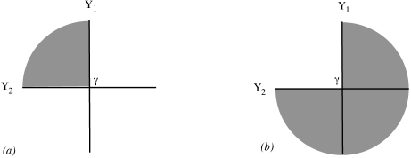
Figure 2. Local configurations for the corner of a pocket $X_{Y_{1}}$ near a boundary curve $\gamma$. $X_{Y_{1}}$ is shaded.

In case (b), there is a component $W$ of $R_{2}\setminus C$ contained in $int(X_{Y_{1}})$, since $W$ cannot intersect $\partial X_{Y_{1}}=Y_{1}\cup Y_{2}$, whose closure contains $\gamma$. Thus $W$ is homotopic into $Y_{1}$, but this can only be if $W$ is an annulus adjacent to $Y_{2}$. The second boundary component of $W$ can not be contained in $Y_{2}$ or $Y_{1}$ by definition, nor can it be in $\partial Y_{1}$ since then $Y_{1}$ and $Y_{2}$ would also be annuli (and there is one annulus in $R_{2}-C$ in each homotopy class). Thus we have a contradiction and case(b) cannot hold.

Now we can show that, in fact, $int(Y_{2})$ cannot meet $C$. For if a component $\beta$ of $C$ were contained in $int(Y_{2})$, there would be a component $W^{\prime}$ of $R_{1}\setminus C$ contained in $int(X_{Y_{1}})$ with one boundary component in $Y_{2}$. As in the previous paragraph $W^{\prime}$ has to be an annulus, in the homotopy class of some $\gamma$ in $\partial Y_{1}$. Since there are at most 2 components of $C$ in a homotopy class, the second boundary component of $W^{\prime}$ must be $\gamma$ itself, but this is impossible since we have ruled out case (b) of Figure 2.

From the above, we see that if $int(Y_{1})$ and $int(Y_{1}^{\prime})$ are any two components of $R_{1}\setminus C$, then the associated pockets $X_{Y_{1}}$ and $X_{Y^{\prime}_{1}}$ are disjoint except possibly along common boundary curves of $Y_{1}$ and $Y^{\prime}_{1}$; any other intersection would lead to the case (b) configuration or to components of $C$ in $int(Y_{2})$. Thus we obtain the desired pocket decomposition of conclusion (4).

In general, some non-annular components of $R_{1}\setminus C$ may have homotopic boundaries. There is a double cover of $S$ such that each non-annular component of $R_{1}\setminus C$ lifts to two homeomorphic components that do not have homotopic boundaries, and the surface in the isotopy class of $R_{1}$ has a connected lift. We can repeat the previous arguments in the corresponding double cover $\widetilde{M}$ of $M$, and obtain a pocket decomposition $\widetilde{\mathcal{X}}$ there. Every pocket of $\widetilde{\mathcal{X}}$ must embed under the double cover, since there can be no new intersection curves. For the same reason, pockets downstairs do not intersect except in the expected way along curves of $C$. Therefore ${\mathcal{X}}$ is a pocket decomposition. ∎

3.6. Proof of Theorem 3.11

We are now prepared to give the proof of Theorem 3.11, which we restate for the reader’s convenience.

Theorem 3.11 (Scaffold Isotopy) Let $\Sigma$ be a straight scaffold, and let $f:\Sigma\to\widehat{M}$ be a good scaffold map. There exists an isotopy $H:\widehat{M}\times[0,1]\to\widehat{M}$ such that $H_{0}=id$, $H_{1}\circ f(\Sigma)=\Sigma$, and $H_{1}\circ f$ is the identity on ${\mathcal{F}}_{\Sigma}$.

Outline

We reduce to the case that $f({\mathcal{V}}_{\Sigma})={\mathcal{V}}_{\Sigma}$, and then consider the intersections of $f({\mathcal{F}}_{\Sigma})$ and ${\mathcal{F}}_{\Sigma}$. We wish to progressively simplify these intersections using the information provided by Lemma 3.14. That lemma describes embedded surfaces with common boundary, whereas the surfaces of ${\mathcal{F}}_{\Sigma}$ and $f({\mathcal{F}}_{\Sigma})$ have disjoint boundaries that meet solid tori, and are wrapped around these solid tori in possibly complicated ways. Hence as a first step we extend the surfaces into the solid tori so as to obtain surfaces whose boundaries meet at the cores.

We can then use Lemma 3.14 to analyze the pockets that arise and simplify them. The main new complication to keep in mind here is the structure of the intersections of the pockets with the solid tori.

Proof.

Let ${\mathcal{F}}={\mathcal{F}}_{\Sigma}$ and ${\mathcal{V}}={\mathcal{V}}_{\Sigma}$. We first reduce to the case that $f({\mathcal{V}})={\mathcal{V}}$.

By assumption, $\Sigma^{\prime}=f(\Sigma)$ is a scaffold so there is a map $\Phi:\widehat{M}\to\widehat{M}$ isotopic to the identity, such that $\Phi({\mathcal{V}}_{\Sigma^{\prime}})$ is a union of tori of the form $\operatorname{\overline{\mathbf{collar}}}(v)\times J_{v}$ with $J_{v}$ an interval. Since $\Sigma$ is straight and $f$ is homotopic to the identity, ${\mathcal{V}}$ is also a union of tori of the form $\operatorname{\overline{\mathbf{collar}}}(v)\times I_{v}$, where the set of homotopy classes $v$ is the same. It remains to construct a further isotopy which takes $\operatorname{\overline{\mathbf{collar}}}(v)\times J_{v}$ to $\operatorname{\overline{\mathbf{collar}}}(v)\times I_{v}$ for each $v$.

Let $h_{v}:J_{v}\to I_{v}$ be an affine orientation preserving homeomorphism, and let $g_{v,t}(x)=(1-t)x+th_{v}(x)$. Thus $g_{v,t}$ ($t\in[0,1]$) is an “affine slide” of $J_{v}$ to $I_{v}$. This allows us to define a family of maps $G_{t}$ on the tubes of $\Phi({\mathcal{V}}_{\Sigma^{\prime}})$, so that for each homotopy class $v$ the restriction of $G_{t}$ to $\operatorname{\overline{\mathbf{collar}}}(v)\times J_{v}$ is $G_{t}(p,x)=(p,g_{v,t}(x))$. This slides $\operatorname{\overline{\mathbf{collar}}}(v)\times J_{v}$ to $\operatorname{\overline{\mathbf{collar}}}(v)\times I_{v}$.

If $v$ and $w$ are disjoint, so are their collars and the $G_{t}$-images of the corresponding tubes do not collide.

Whenever $v$ and $w$ overlap, $J_{v}\cap J_{w}=\emptyset$, and $I_{v}\cap I_{w}=\emptyset$. Supposing $\max J_{v}<\min J_{w}$, the order-preserving property of $f$ implies that $\max I_{v}<\min I_{w}$. Thus it follows that $g_{v,t}(J_{v})$ and $g_{w,t}(J_{w})$ are disjoint for any $t$, and again the images of the corresponding tubes do not collide.

By the isotopy extension theorem [67], this isotopy of $\Phi({\mathcal{V}}_{\Sigma^{\prime}})$ can be extended to an isotopy $\Psi_{t}$ of $\widehat{M}$.

Thus, after replacing $f$ with $\Psi_{1}\circ\Phi\circ f$, we may from now on assume that ${\mathcal{V}}_{\Sigma^{\prime}}={\mathcal{V}}$. We will build an isotopy of maps of pairs

$$H:(\widehat{M}\times[0,1],{\mathcal{V}}\times[0,1])\to(\widehat{M},{\mathcal{V}})$$

such that $H_{0}=id$ and $H_{1}\circ f$ is the identity on ${\mathcal{F}}$. This will be done by induction on the pieces of ${\mathcal{F}}$.

In the inductive step, we may assume that on some union of components ${\mathcal{E}}\subset{\mathcal{F}}$, $f$ is already equal to the identity. We let $R$ be a component of ${\mathcal{F}}\setminus{\mathcal{E}}$, and build an isotopy of pairs $(\widehat{M},{\mathcal{V}})$ which fixes pointwise a neighborhood of ${\mathcal{E}}$, and moves $f|_{R}$ to the identity.

Our first step is to apply an isotopy so that $\partial R$ and $f(\partial R)$ are disjoint. Let $\gamma$ be a boundary component of $R$, lying in the boundary of a solid torus $V$ in ${\mathcal{V}}$, and let $\gamma^{\prime}$ be a component of $f(\partial R)$ lying in $\partial V$.

By Lemma 3.6, since both $\Sigma$ and $f(\Sigma)$ are scaffolds, both $\gamma$ and $\gamma^{\prime}$ are in the homotopy class of level curves and hence homotopic to each other in $\partial V$. We claim that they are isotopic, within $\partial V\setminus{\mathcal{E}}$, to disjoint curves. If they are in different components of $\partial V\setminus{\mathcal{E}}$ then they are already disjoint. If they are in the same component $A$, then $A$ is either an annulus or a torus in which $\gamma^{\prime}$ and $\gamma$ are homotopic, so $\gamma^{\prime}$ is isotopic within $A$ to a curve disjoint from $\gamma$.

This isotopy may be extended to a small neighborhood of $\partial V$ to have support in the complement of ${\mathcal{E}}$, so after applying this isotopy to $f$ we may assume that $\partial R$ and $f(\partial R)$ are disjoint.

Now, in order to apply Lemma 3.14, let us enlarge $R$ and $f(R)$ to surfaces $R_{1}$ and $R_{2}$, as follows. If $V$ is a component of ${\mathcal{V}}$ meeting just one boundary component $\gamma$ of $R$, let $A_{1}$ and $A_{2}$ be embedded annuli in $V$ joining $\gamma$ and $f(\gamma)$, respectively, to a fixed core curve of $V$, and let $A_{1}$ and $A_{2}$ be disjoint except at the core. If $V$ meets two components of $\partial R$, join them with an embedded annulus $A_{1}$, and similarly join the corresponding pair of components of $f(\partial R)$ with an embedded $A_{2}$, so that $A_{1}$ and $A_{2}$ intersect transversely and minimally – either not at all, or transversely in one core curve. Figure 3 illustrates these possibilities. Repeating for each $V$, let $R_{1}$ be the union of $R$ with all the annuli $A_{1}$, and let $R_{2}$ be the union of $f(R)$ with all the annuli $A_{2}$.

Since $R$ is a level surface, we may choose the annuli $A_{1}$ to be level, so that $R_{1}$ is still a level surface.

Figure 3. The three ways in which annuli are added to $R$ and $f(R)$. To obtain the true picture, cross each diagram with $S^{1}$.

Because we have joined homotopic pairs of boundary components, $R_{1}$ and $R_{2}$ satisfy the conditions of Lemma 3.14. Let ${\mathcal{X}}$ be the collection of pockets described in the lemma. For each of the possible cases we will describe how to simplify the picture by an isotopy of $(M,{\mathcal{V}})$. The general move, given a pocket $X$ bounded by $Y_{1}\subset R_{1}$ and $Y_{2}\subset R_{2}$, is to apply an isotopy in a neighborhood of $X$ which pushes $Y_{2}$ off $R_{1}$ using the product structure of the pocket. However we have to be careful to deal correctly with the possible intersections of $X$ with ${\mathcal{E}}$ and ${\mathcal{V}}$. In particular we will maintain inductively the property that the intersection of $R_{1}\cup R_{2}$ with each solid torus is always one of the configurations in Figure 3.

1: Suppose ${\mathcal{X}}$ contains a disk pocket $X$. Since $X$ is a ball, no component of ${\mathcal{V}}$ or ${\mathcal{E}}$ can be contained in it. ${\mathcal{E}}$ is disjoint from $R_{1}$ and $R_{2}$ and hence cannot intersect $X$ at all. Since according to Figure 3 any intersection curve of $V$ with $R_{1}\cup R_{2}$ is homotopically nontrivial, ${\mathcal{V}}$ cannot intersect $\partial X$, and hence $X$, either. Hence $R_{2}$ can be isotoped through $X$, reducing the number of intersections, and the isotopy is the identity on ${\mathcal{V}}$ and ${\mathcal{E}}$. After a finite number of such moves we may assume there are no disk pockets.

2: Suppose ${\mathcal{X}}$ contains two homotopic non-peripheral annulus pockets $X$ and $X^{\prime}$, with interiors disjoint from each other and from $R_{1}$ and $R_{2}$, and on opposite sides of $R_{1}$.

If one of the annulus pockets misses ${\mathcal{V}}$ then it cannot meet any component of ${\mathcal{E}}$, and hence we may isotope across it to reduce the number of intersection curves.

If both of the pockets meet ${\mathcal{V}}$, it must be in a single solid torus $V$ in the same homotopy class. By the inductive hypothesis, the intersections with $V$ must be as in Figure 3, so that $X$ and $X^{\prime}$ each meet $V$ in a solid torus. There are two intersection patterns in $V$, depicted in Figure 4. In case (a), $X$ and $X^{\prime}$ intersect at the core curve of $V$. The product structure in $X$ can be chosen so that $\partial V\cap X$ is vertical, and again we can isotope through $X$, preserving $V$, to reduce the number of intersection curves.

Figure 4. The two ways that a solid torus $V$ can intersect two homotopic annulus pockets.

In case (b), $X$ and $X^{\prime}$ do not intersect in $V$ and we have to consider the picture more globally. Since $X$ and $X^{\prime}$ meet $R_{1}$ on opposite sides, the possible configurations are as in Figure 5 (up to orientation). In each case, $X$ meets $V$ in a region bounded by a subset of $R_{2}$, and $X^{\prime}$ meets $V$ in a region bounded by a subset of $R_{1}$. Outside $V$ there is a solid torus $Z$ bounded by three annuli, one in $\partial V$, one in $\partial X$ and one in $R_{1}$, and $int(Z)$ is disjoint from $R_{1}$. In the top case, $int(Z)$ is disjoint from $R_{2}$ and we may push the annulus $\partial Z\cap\partial X$ across the rest of $Z$, thus reducing the number of intersection curves outside ${\mathcal{V}}$ (although we introduce an intersection in $V$, as shown).

In the bottom case, we can find an innermost annulus of $R_{2}\cap Z$, and push across the resulting pocket. Note that in these cases the isotopy can be done in the complement of ${\mathcal{E}}$ since no component of ${\mathcal{E}}$ can be contained in a solid torus.

After a finite number of such moves we may assume that ${\mathcal{X}}$ does not contain a pair of homotopic non-peripheral annulus pockets.

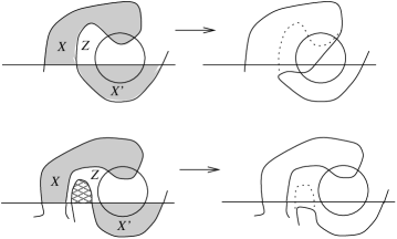
Figure 5. The two possible moves in case (b)

3: If ${\mathcal{X}}$ contains a peripheral annulus pocket $X$, let $V$ denote the component of ${\mathcal{V}}$ in the same homotopy class. The intersection of $\partial V$ with $R_{1}$ and $R_{2}$ must be as in the first picture in Figure 3. We can adjust the product structure of the pocket so that $\partial V$ is vertical, and hence we can isotope $Y_{2}$ off of $Y_{1}$ while preserving $V$ (see figure 6). Again, this can be done in the complement of ${\mathcal{E}}$.

Figure 6. A peripheral annulus pocket can only intersect $V$ as shown (multiplied by $S^{1}$). The isotopy move is shown as well.

4: If ${\mathcal{X}}$ is a pocket decomposition, we first claim that no pocket contains all of a component of ${\mathcal{V}}$ or ${\mathcal{E}}$. Suppose that $X\in{\mathcal{X}}$ does contain such a component $Z$. We will obtain a contradiction to the order-preserving properties of the map $f$.

$Z$ is homotopic into $R_{1}$, and we claim it must also overlap $R$ – the alternative is that $Z$ is homotopic to one of the annuli in $R_{1}\setminus R$ – but then it would have to be one of the solid tori that intersect $R_{1}$, contradicting the fact that $Z$ lies within $X$.

Recall that $R_{1}$ is a level surface, let $Y_{1}$ be the subsurface of $R_{1}$ in the boundary of $X$, and assume without loss of generality that $X$ is adjacent to $R_{1}$ from below. Because $R_{1}$ is a level surface $Z$ can be pushed to $-\infty$ in the complement of $R_{1}$. Since $Z$ overlaps $R$ and $\Sigma$ is straight, they are ordered and so $Z\prec_{\rm top}R$. Since $f$ is a good scaffold map we have $f(Z)\prec_{\rm top}f(R)$, but $f(Z)=Z$ so $Z\prec_{\rm top}f(R)$.

There is an isotopy of $M$ supported on a small neighborhood of the pockets different from $X$, which pushes all of them outside of the region above $Y_{1}$, which we can call $Y_{1}\times(t,\infty)$. Let $\Psi$ be the end result of this isotopy. We can push $Z$ through the product structure of $X$ to just above $Y_{1}$, and then to $+\infty$ through the region $\Psi^{-1}(Y_{1}\times(t,\infty))$, avoiding $R_{2}$ and in particular $f(R)$ (figure 7). This contradicts $Z\prec_{\rm top}f(R)$.

Figure 7. If $Z$ is contained in a pocket, it contradicts order preservation.

The only remaining issue is that a pocket $X$ might intersect, but not contain, one of the solid tori $V$. A priori there are six possible intersection patterns of $V$ with the pockets, as in figure 8.

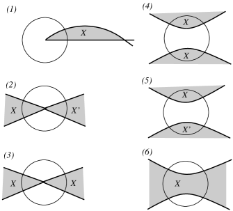
Figure 8. The six intersection patterns of a pocket $X$ with a tube $V$

In case (1), $V$ corresponds to a peripheral homotopy class in $R_{1}$ and $X$ meets $V$ in a solid torus with the core of $V$ at its boundary. The product structure of $X$ can be adjusted so that the annulus $\partial V\cap X$ is vertical. (This is similar to the peripheral annulus pocket case.)

In case (2), $V$ meets two pockets $X$ and $X^{\prime}$ and there is an intersection curve in the core of $V$. Again $\partial V\cap X$ can be made vertical.

In case (3), the local pattern is the same as in case (2) but we consider the possibility that both intersections are part of $X$. This case cannot occur: The orientation of $X$ induced from $M$ induces an orientation on each of the two boundary surfaces $Y_{1}$ and $Y_{2}$. However in the local picture in $V$, each $Y_{i}$ inherits inconsistent orientation from the two sides, since $Y_{1}$ and $Y_{2}$ intersect transversely.

In case (4), $X$ meets $V$ in two disjoint solid tori. This case can also be ruled out: Consider an annulus $A$ in $V$ with homotopically nontrivial boundaries in the two components of $X\cap V$. Because $X$ is a pocket, and the map of $S$ to $M$ is a homotopy-equivalence, the boundaries of $A$ can also be joined by an annulus $A^{\prime}$ in $X$. This produces a torus that intersects the level surface $R_{1}$ in exactly one, essential, curve $\gamma$. The curve is in the homotopy class of $V$, which in this case is non-peripheral in $R_{1}$. But this is impossible: Let $S_{1}$ be the full level surface containing $R_{1}$. Any intersection of the torus with $S_{1}\setminus R_{1}$ cannot be essential because then it would be homotopic to $\gamma$, which is nonperipheral in $R_{1}$. The nonessential intersections can be removed by surgeries, yielding a torus that cuts through $S_{1}$ in just one curve – but $S_{1}$ separates $M$, a contradiction.

In case (5), $V$ meets $X$ and $X^{\prime}$ in disjoint solid tori. Hence $V$ must be homotopic to a boundary component of $X$ and of $X^{\prime}$. This gives us a configuration which agrees, in a neighborhood of $V$, with the top picture in figure 5 – the only difference is that one of the pockets is not an annulus pocket now. (Notice that the bottom picture in figure 5 cannot occur, since we have assumed that $C=R_{1}\cap R_{2}$ never contains more than 2 homotopic curves.) The same isotopy move as in figure 5 simplifies the situation by reducing the number of intersection curves outside of ${\mathcal{V}}$ (and changing the local configuration at $V$ to case (2)).

In case (6), $V$ intersects $\partial X$ in two disjoint annuli. The intersection $V\cap X$ is a solid torus $Z$, and the product structure of $X$ can be adjusted so that the two annuli of $\partial Z\cap\partial V$ are vertical. (This is essentially because in a product $R\times[0,1]$ there is only one isotopy class of embedded annulus for each isotopy class in $R$.)

In conclusion: cases (3) and (4) do not occur. Case (5) can be removed locally, yielding a simpler situation. Hence we can assume that all pockets only intersect ${\mathcal{V}}$ in the patterns of cases (1), (2) and (6). The product structure of each pocket $X$ can then be adjusted so that all the annuli of the form $\partial V\cap X$ are simultaneously vertical, and then a single push of $R_{2}$ through each pocket yields an isotopy of $(M,{\mathcal{V}})$ that takes $R_{2}$ to $R_{1}$, and $f(R)$ to $R$, and fixes a neighborhood of ${\mathcal{E}}$. A final isotopy within $R$ takes $f$ to the identity. This completes the proof of Theorem 3.11. ∎

3.7. Wrapping coefficients

In this section, we develop a criterion to guarantee that a surface is embedded which will be used in the proof of Theorem 6.2. Roughly, we show that if a surface is embedded off of an annulus immersed in the boundary of a tube, and is homotopic to $+\infty$ or $-\infty$ in the complement of that tube, then the surface is embedded.

Lemma 3.15.

Let $R\subseteq S$ be an essential subsurface and $V$ a solid torus in $\operatorname{{\mathbf{emb}}}(M)$ homotopic to a nonperipheral curve $\gamma$ in $R$. Let $R^{\prime}=R\setminus\operatorname{\mathbf{collar}}(\gamma)$. Suppose that $h\in\operatorname{{\mathbf{map}}}(R,M)$ is a map such that $h|_{R^{\prime}}$ is an embedding into $M\setminus int(V)$ with $h^{-1}(\partial V)=\operatorname{\overline{\mathbf{collar}}}(\gamma)$, $h(\partial R^{\prime})$ is unknotted and unlinked, and $h|_{\operatorname{\mathbf{collar}}(\gamma)}$ is an immersion of $\operatorname{\mathbf{collar}}(\gamma)$ in $\partial V$.

If $h$ is homotopic to either $-\infty$ or to $+\infty$ in the complement of $int(V)$ then $h|_{\operatorname{\mathbf{collar}}(\gamma)}$ (and hence $h$ itself) is an embedding.

We first define an algebraic measure of wrapping. Suppose that $V$ is a straight solid torus in $M$, $R\subseteq S$ is an essential subsurface, and the core of $V$ is homotopic to a nonperipheral curve in $R$. Consider $f\in\operatorname{{\mathbf{map}}}(R,M)$ whose image is disjoint from $int(V)$, and suppose that $f(\partial R)$ is not linked with $V$, which means that $f|_{\partial R}$ is homotopic to both $-\infty$ and $+\infty$ in the complement of $V$. (Note that it is sufficient to assume it is homotopic to $-\infty$ in the complement of $V$: since $V$ is nonperipheral in $R$ and straight, $\partial R\times{\mathbb{R}}$ is disjoint from $V$, so once $f(\partial R)$ is pushed far enough below it can be pushed above along $\partial R\times{\mathbb{R}}$).

We then define a “wrapping coefficient” $d_{-}(f,V)\in{\mathbb{Z}}$ as follows: Let $r\in{\mathbb{R}}$ be smaller than the minimal level of $V$, and let $G:R\times[0,1]\to M$ be a homotopy with $G_{0}=s_{r}:R\to R\times\{r\}$, and $G_{1}=f$. By the unlinking assumption on $f(\partial R)$ we may choose $G$ so that $G(\partial R\times[0,1])$ is disjoint from $int(V)$. Then the degree of $G$ over $int(V)$ is well-defined, and we denote it $\deg(G,V)$.

If $G^{\prime}$ is another such map we claim $\deg(G,V)=\deg(G^{\prime},V)$. Viewing $G$ and $G^{\prime}$ as 3-chains, the difference $G-G^{\prime}$ has boundary equal to $G(\partial R\times[0,1])-G^{\prime}(\partial R\times[0,1])$, a union of singular tori. Since $M\setminus V$ is atoroidal and these tori are not homotopic to $\partial V$, they must bound a union of (singular) solid tori $W$ in the complement of $V$, and we can write $\partial(G-G^{\prime}-W)=0$. Since $H_{3}(M)=\{0\}$ we know $\deg(G-G^{\prime}-W,V)=0$ and since the contribution from $W$ is $0$ we must have $\deg(G,V)=\deg(G^{\prime},V)$. Thus we are justified in defining $d_{-}(f,V)\equiv\deg(G,V)$. We also drop $V$ from the notation, writing $d_{-}(f)$, $deg(G)$ etc, where convenient.

It is clear that $d_{-}(s_{r})=0$ and, more generally, that if $f$ is deformable to $-\infty$ in the complement of $V$ then $d_{-}(f)=0$. Furthermore if $H$ is a homotopy such that $H(\partial R\times[0,1])$ is disjoint from $V$, $H_{0}=f$, $H_{1}=g$, and $f(R)$ and $g(R)$ are disjoint from $V$, then

$$d_{-}(g)-d_{-}(f)=\deg(H).$$ (3.3)

We can define $d_{+}(f)$ similarly as $\deg(G)$, where $G$ is a homotopy such that $G_{0}=f$ and $G_{1}=s_{t}$, with $t$ larger than the top of $V$. Then $d_{+}(f)$ must be $0$ for $f$ to be deformable to $+\infty$ in the complement of $V$.

Proof of Lemma 3.15.

Since $h(\partial R^{\prime})$ is unknotted and unlinked we may attach solid tori to the boundary components of $h(\partial R)$ so that, together with $V$ and $h(R^{\prime})$, we have a scaffold $\Sigma$. (Notice that since each component of $h(\partial R^{\prime})\cap\partial V$ is a simple closed curve which represents an indivisible element of $\pi_{1}(M)$, it must be isotopic to the core curve of $V$.) Since $\Sigma$ has no overlapping pieces, it is combinatorially straight. By Lemma 3.12 we may assume, after re-identifying $M$ with $S\times{\mathbb{R}}$, that $V$ is a straight solid torus and $h(R^{\prime})$ is a level surface. Assume without loss of generality that $h$ is homotopic to $-\infty$ in the complement of $V$.

Let $A_{-}$ be the annulus in $\partial V$ consisting of the part of the boundary below $h(R^{\prime})$, and let $h_{-}:R\to M$ be an extension of $h|_{R^{\prime}}$ that maps $\operatorname{\mathbf{collar}}(\gamma)$ to $A_{-}$ and is an embedding.

Clearly $h_{-}$ is deformable to $-\infty$ in the complement of $V$, and hence $d_{-}(h_{-})=0$. Similarly, $d_{-}(h)=0$.

The difference between $h(\operatorname{\mathbf{collar}}(\gamma))$ and $h_{-}(\operatorname{\mathbf{collar}}(\gamma))$, considered as 2-chains, gives a cycle $k[\partial V]$ with $k\in{\mathbb{Z}}$. We immediately have $d_{-}(h)=d_{-}(h_{-})+k=k$. Since $d_{-}(h)=d_{-}(h_{-})=0$, we conclude that $k=0$. This implies that, since $h$ and $h_{-}$ are both immersions on $\operatorname{\mathbf{collar}}(\gamma)$ which agree on $\partial\operatorname{\mathbf{collar}}(\gamma)$, they must have the same image. It follows that $h|_{\operatorname{\mathbf{collar}}(\gamma)}$ is an embedding. ∎

3.8. Some ordering lemmas

We now apply the scaffold machinery to obtain some basic properties of the $\prec_{\rm top}$ relation. All these properties will be used in the proof of Lemma 8.4, which allows us to choose a cut system whose images under the, suitably altered, model map are correctly ordered.

The following lemma gives us a transitivity property for $\prec_{\rm top}$ in some special situations.

Lemma 3.16.

Let $R_{1}$ and $R_{2}$ be disjoint homotopic surfaces in $\operatorname{{\mathbf{emb}}}(M)$. Let ${\mathcal{V}}$ be an unlinked unknotted collection of solid tori in $M$ with one component for each homotopy class of component of $\partial R_{1}$, so that $\partial R_{1}$ and $\partial R_{2}$ are embedded in $\partial{\mathcal{V}}$.

1. $R_{1}$ and $R_{2}$ are $\prec_{\rm top}$-ordered.

2. Let $Q\in\operatorname{{\mathbf{emb}}}(M)$ be disjoint from $R_{1}\cup R_{2}\cup{\mathcal{V}}$, so that the domain of $Q$ is contained in the domain $R$ of $R_{1}$ and $R_{2}$.

   Suppose that $R_{1}\prec_{\rm top}Q$ and $Q\prec_{\rm top}R_{2}$. Then $R_{1}\prec_{\rm top}R_{2}$.

Proof.

Let $\Sigma$ denote the scaffold with ${\mathcal{F}}_{\Sigma}=R_{1}$ and ${\mathcal{V}}_{\Sigma}={\mathcal{V}}$. $\Sigma$ has no overlapping pieces, so it is combinatorially straight. Using the straightening lemma 3.12, after an isotopy we may assume that $\Sigma$ is straight.

Now the Pocket Lemma 3.13 implies that there is a product region $X$ homeomorphic to $R\times[0,1]$ whose boundary consists of $R_{1}$, $R_{2}$, and annuli in the tubes of ${\mathcal{V}}_{\Sigma}$ associated to their boundaries. Thus $R_{2}$ is isotopic to $R_{1}$ by an isotopy keeping the boundaries in ${\mathcal{V}}$, so that we may assume that $X$ is actually equal to $R\times[0,1]$ in $M=S\times{\mathbb{R}}$, with $R_{1}\cup R_{2}=R\times\{0,1\}$. It follows from this that if $R_{1}=R\times\{0\}$ then $R_{1}\prec_{\rm top}R_{2}$, and if $R_{1}=R\times\{1\}$ then $R_{2}\prec_{\rm top}R_{1}$. Hence we have part (1).

It remains to show that, given the hypothesis on $Q$, $R_{1}=R\times\{0\}$, from which $R_{1}\prec_{\rm top}R_{2}$ and hence (2) follows.

If $Q\subset X$ then we must have $R\times\{0\}\prec_{\rm top}Q$ and $Q\prec_{\rm top}R\times\{1\}$, so we are done.

Now let us suppose that $Q$ is in the complement of $X$, and obtain a contradiction. The condition $R_{1}\prec_{\rm top}Q$ implies that there exists a homotopy $H:Q\times[0,\infty)\to M$ such that $H(Q\times\{t\})$ goes to $+\infty$ as $t\to+\infty$, and which avoids $R_{1}$. We claim that $H$ can be chosen to avoid $R_{2}$ as well. Let $W$ be a neighborhood of $X$ disjoint from $Q$. There is a homeomorphism $\phi$ taking $M\setminus R_{1}$ to $M\setminus X$, which is the identity outside $W$. Thus $\phi\circ H$ is the desired homotopy. This contradicts $Q\prec_{\rm top}R_{2}$, so again we are done. ∎

The next lemma tells us that for disjoint overlapping non-homotopic non-annular surfaces with boundary in an unknotted and unlinked collection of solid tori, the $\prec_{\rm top}$-ordering is determined by their boundaries.

Lemma 3.17.

Let $P,R\in\operatorname{{\mathbf{emb}}}(M)$ be disjoint overlapping non-homotopic non-annular surfaces such that $\partial R\cup\partial P$ is embedded in a collection ${\mathcal{V}}$ of unknotted, unlinked, homotopically distinct solid tori, so that each component of ${\mathcal{V}}$ intersects $\partial P$ or $\partial R$, and ${\mathcal{V}}\cap(int(R)\cup int(P))=\emptyset$. Suppose that for each component $\alpha$ of $\partial R$ that overlaps $P$ we have $\alpha\prec_{\rm top}P$, and for each component $\beta$ of $\partial P$ that overlaps $R$ we have $R\prec_{\rm top}\beta$. Then $R\prec_{\rm top}P$.

Proof.

Assume, possibly renaming $P$ and $R$ and reversing directions, that the domain of $R$ is not contained in the domain of $P$.

Let $\Sigma$ be the scaffold with ${\mathcal{F}}_{\Sigma}=R$ and ${\mathcal{V}}_{\Sigma}={\mathcal{V}}$. By hypothesis ${\mathcal{V}}$ is isotopic to a union of straight solid tori, so that $\prec_{\rm top}|_{\mathcal{V}}$ is acyclic and satisfies the overlap condition. Since the hypotheses also give us that $R\prec_{\rm top}V$ for each component $V$ of ${\mathcal{V}}$ that overlaps $R$ we conclude that $\prec_{\rm top}|_{\Sigma}$ is still acyclic and satisfies the overlap condition. Hence $\Sigma$ is combinatorially straight and by Lemma 3.12, after isotopy we may assume that $\Sigma$ is straight.

In particular we may assume that $R=R^{\prime}\times\{0\}$. Let $X=R^{\prime}\times(-\infty,0]$.

After pushing $\partial P$ in $\partial{\mathcal{V}}$ (by an isotopy supported in a small neighborhood of ${\mathcal{V}}$ and leaving $\Sigma$ invariant) we may assume that $\partial P$ is outside of $X$.

Now consider $P\cap\partial X=P\cap\partial R^{\prime}\times(-\infty,0]$ (we may assume this intersection is transverse). All inessential curves bound disks in both $P$ and $\partial X$, and so an isotopy of $P$ will remove them. The remaining curves are in the homotopy classes of the components of $\partial R^{\prime}$. Let $A$ be a component of $P\cap X$. If $A$ is an annulus then it and an annulus in $\partial X$ bound a solid torus (annulus pocket) in $X$, and taking an innermost such solid torus we may remove it by an isotopy of $P$ without producing new intersection curves with $\partial X$. After finitely many moves we may assume there are no annular intersections.

Any non-annular $A$ must be a subsurface of $P$, and hence is the image of a subsurface $A^{\prime}$ of $S$. On the other hand, $A\subset X$ implies that $A^{\prime}$ is homotopic into $R^{\prime}$, and $\partial A\subset\partial X$ implies that $\partial A^{\prime}$ is homotopic into $\partial R^{\prime}$. Since $A^{\prime}$ is not an annulus, the only way this can happen is if $A^{\prime}$ is isotopic to $R^{\prime}$ (see, for example, Theorem 13.1 in [34].) But this contradicts the assumption that the domain of $R$ is not contained in the domain of $P$. Thus there is no non-annular component $A$.

We conclude that, after an isotopy that does not move $R$, $P$ may be assumed to lie outside of $X$. Thus $P$ is homotopic to $+\infty$ avoiding $X$ and hence $R$, and $R$ is homotopic to $-\infty$ (through $X$) in the complement of $P$. $R$ and $P$ overlap, so we conclude by Lemma 3.1 that $R\prec_{\rm top}P$. ∎

The next lemma will allow us to check more easily that tubes are ordered with respect to non-annular embedded surfaces with boundary in a collection of straight solid tori.

Lemma 3.18.

Let $R\in\operatorname{{\mathbf{emb}}}(M)$ be non-annular, with boundary embedded in a collection ${\mathcal{V}}$ of straight solid tori. Let $U$ be a straight solid torus disjoint from $R\cup{\mathcal{V}}$ and overlapping $R$. If $R$ is homotopic to $-\infty$ in the complement of $U$ then $R\prec_{\rm top}U$, and if $R$ is homotopic to $+\infty$ in the complement of $U$ then $U\prec_{\rm top}R$.

Proof.

Assume without loss of generality that $R$ is homotopic to $-\infty$ in the complement of $U$. Let $B=\gamma\times[t,\infty)$ where $\gamma\times\{t\}$ is embedded in $\partial U$ and homotopic to the core of $U$. Since $U$ and ${\mathcal{V}}$ are straight and ${\mathcal{V}}$ is homotopic to $-\infty$ in the complement of $U$ (since $R$ is), $B$ must be disjoint from ${\mathcal{V}}$. We may assume that $B$ intersects $R$ transversely, so that components of $B\cap R$ are either homotopically trivial or homotopic to the core of $U$.

Homotopically trivial components may be removed by isotopy of $B$. The nontrivial components are signed via the natural orientation of $B$ and $R$, and the fact that $R$ is homotopic to $-\infty$ in the complement of $U$ means that the signs sum up to 0. Two components of opposite signs that are adjacent on $B$ can be removed by an isotopy of $B$, and we conclude that $B$ can be isotoped away from $R$. Thus $U$ is homotopic to $+\infty$ in the complement of $R$, and we conclude (invoking Lemma 3.1) that $R\prec_{\rm top}U$. ∎

4. Cut systems and partial orders

In this section, we link combinatorial information from the hierarchy $H$ to topological ordering information of split-level surfaces in $M_{\nu}$. A split-level surface is an embedded surface in the model manifold associated to a slice of $H$ that is made up of level subsurfaces arising as the upper and lower boundaries of blocks in the model. As these split-level surfaces and their images in $M$ will play an important role in what follows, we now develop some control over them and their interactions within the model, aiming in particular for a consistency result (Proposition 4.15) comparing topological ordering in $M_{\nu}$ and a more combinatorial ordering we define on corresponding slices in $H$.

This consistency result will not apply generally to all slices in $H$ and their associated domains, but after a thinning procedure we arrive at a collection of slices called a cut system whose split-level surfaces are well behaved with respect to the topological partial ordering and divide the model into regions of controlled size as we will see in §5.

4.1. Split-level surfaces associated to slices

If $a$ is a slice of $H$, we recall from Section 2.2 that $g_{a}$ denotes its bottom geodesic and $v_{a}$ is the bottom simplex of $a$. Then $p_{a}=(g_{a},v_{a})$ is the bottom pair of $a$. Let

$$D(a)=D(p_{a})=D(g_{a})$$

be the domain of $g_{a}$. If $D(a)$ is not an annulus, let

$$\check{D}(a)=D(a)\setminus\operatorname{\mathbf{collar}}(\operatorname{base}(a))$$

be the complement in $D(a)$ of the standard annular neighborhoods of the curves in $\operatorname{base}(a)$. When $a$ is a saturated slice, the subsurface $\check{D}(a)\subset D(a)$ is a collection of pairwise disjoint 3-holed spheres. If $D(a)$ is an annulus, we let $\check{D}(a)=D(a)$.

Each slice in $H$ gives rise to a properly embedded surface in $M_{\nu}[0]$ called a split-level surface. Given a non-annular slice $a$ of $H$, each 3-holed sphere $Y\subset\check{D}(a)$ admits a natural level embedding $F_{Y}\subset M_{\nu}[0]$. This embedded copy $F_{Y}$ of $Y$ lies in the top boundary and the bottom boundary of the two blocks that are glued along $F_{Y}$. The split-level surface $F_{a}$ associated to $a$ is obtained by letting

$$F_{a}=\bigcup_{Y\subset\check{D}(a)}F_{Y}.$$

Given a slice $a$ and $v\in\operatorname{base}(a)$, we say $\gamma_{v}$ is a hyperbolic base curve for $a$ if there is a solid torus $U(v)$ in $M_{\nu}[\infty]$ whose closure is compact; otherwise we say $\gamma_{v}$ is a parabolic base curve. For each $v\in a$ with $\gamma_{v}$ a hyperbolic base curve, we extend the above embedding of $\check{D}(a)$ across the annulus $\operatorname{\mathbf{collar}}(v)$ to a map of $\operatorname{\mathbf{collar}}(v)$ into $U(v)$: the core $\gamma_{v}$ is sent to the core of the tube $U(v)$ with its model hyperbolic metric, and the pair of annuli $\operatorname{\mathbf{collar}}(v)\setminus\gamma_{v}$ are mapped in such a way that radial lines in $\operatorname{\mathbf{collar}}(v)$ map to radial geodesics in the tube $U(v)$. Given $v\in\operatorname{base}(a)$ for which $\gamma_{v}$ is a parabolic base curve, we extend across the corresponding annulus $\operatorname{\mathbf{collar}}(\gamma_{v})$ to any embedding of $\operatorname{\mathbf{collar}}(\gamma_{v})$ into $U(v)$.

We remark that given a slice $a$ the only base curves that fail to be hyperbolic correspond to vertices $a\in\operatorname{base}(a)$ for which $v$ is a vertex in $\operatorname{base}(I(H))$ without a transversal or $v$ is a vertex in $\operatorname{base}(T(H))$ without a tranversal.

Extending over each annulus $\operatorname{\mathbf{collar}}(v)$ for $v\in\operatorname{base}(a)$ in this way, we obtain an embedding of $D(a)$ into $M_{\nu}$ whose image we denote by $\widehat{F}_{a}$. For each integer $k\in[0,\infty]$ we denote by $\widehat{F}_{a}[k]$ the intersection

$$\widehat{F}_{a}[k]=\widehat{F}_{a}\cap M_{\nu}[k].$$

We call the surfaces $\widehat{F}_{a}[k]$ extended split-level surfaces.

When $a$ is an annular slice, there is a vertex $v$ so that $D(a)=\overline{\operatorname{\mathbf{collar}}(v)}$. We refer to this vertex $v$ as the core vertex of $a$, and denote it by $v=\operatorname{core}(a)$. Then we have the associated solid torus $U(v)\subset M_{\nu}$. In the interest of comparing all slices in $C$ and their associated topological objects in $M_{\nu}$, we adopt the convention that for each integer $k\in[0,\infty]$ and annular slice $a$ we have

$$F_{a}[k]=\widehat{F}_{a}[k]=\widehat{F}_{a}=U(v).$$

4.2. Resolution sweeps of the model

A resolution $\{\tau_{n}\}$ of the hierarchy $H_{\nu}$ yields a “sweep” of the model manifold by split-level surfaces, which is monotonic with respect to the $\prec_{\rm top}$ relation. More specifically, in §8.2 of [54], the embedding of $M_{\nu}[0]$ in $S\times{\mathbb{R}}$ is constructed inductively using an exhaustion of $M_{\nu}[0]$ by submanifolds $M_{i}^{j}$ that are unions of blocks. Each $F_{\tau_{j}}$ appears as the “top” boundary of $M_{i}^{j}$, so that $int(M_{i}^{j})$ lies below the cross-sectional surface $\widehat{F}_{\tau_{j}}$ in the product structure of $S\times{\mathbb{R}}$. When $\tau_{j}\to\tau_{j+1}$ is a move associated to to a 4-edge $e_{j}$, there is a block $B_{j}=B(e_{j})$ which is appended above $\widehat{F}_{\tau_{j}}$, and $F_{\tau_{j+1}}$ is obtained from $F_{\tau_{j}}$ by replacing the bottom boundary of $B_{j}$ by its top boundary. We say that $B_{j}$ “is appended at time $j$” in the resolution. (For other types of elementary moves the surfaces $\widehat{F}_{\tau_{j}}$ and $\widehat{F}_{\tau_{j+1}}$ are the same.)

The following statement about $\prec_{\rm top}$ is an immediate consequence of this construction, and Lemma 3.1.

Lemma 4.1.

Fix a resolution $\{\tau_{n}\}$ of $H$. If $i<j$ and $W\subset\widehat{F}_{\tau_{i}}$ and $W^{\prime}\subset\widehat{F}_{\tau_{j}}$ are essential subsurfaces which overlap and are disjoint, then $W\prec_{\rm top}W^{\prime}$.

Similarly, if $B$ is appended at time $j>i$ and $W_{B}$ is the middle surface of $B$ then $\widehat{F}_{\tau_{i}}\prec_{\rm top}W_{B}$. If $B$ is appended at time $j<i$ then $W_{B}\prec_{\rm top}\widehat{F}_{\tau_{i}}$.

4.3. Cut systems

Given a collection $C$ of slices of $H$, we let

$$C|_{h}\equiv\{\tau\in C:g_{\tau}=h\}$$

denote the slices in $C$ with bottom geodesic $h$. Let

$$5\leq d_{1}<d_{2}\leq\infty$$

be fixed elements in ${\mathbb{N}}\cup\{\infty\}$. Then the collection $C$ is a cut system satisfying a $(d_{1},d_{2})$ spacing condition if the following hold:

1. Distribution of bottom pairs: For each $h\in H$ with $\xi(D(h))\geq 4$, the set $\{v_{\tau}:\tau\in C|_{h}\}$ of bottom vertices on $h$ cuts $h$ into intervals of length at most $d_{2}$, and, if non-empty, cuts $h$ into at least three intervals of size at least $d_{1}$. Futhermore, no two slices have the same bottom pair, and no $v_{\tau}$ is the first or last simplex of $h$.

2. Initial pairs: For every pair $(h,w)\in\tau\in C$ that is not a bottom pair of $\tau$, $w$ is the first simplex of $h$.

3. Saturation: Each slice $\tau\in C$ with non-annular bottom geodesic is a saturated non-annular slice.

4. Annular cut slices: For any annular geodesic $g$ there is at most one slice $\tau\in C$ with $g_{\tau}=g$.

Note that the spacing condition (1) puts no restriction on annular slices in $C$. An annular slice consists of an annular geodesic and a choice of vertex, but in fact the vertex plays no role in the rest of the argument and is only included for notational consistency.

The following lemma will allow us to exploit the standing assumption that $d_{1}\geq 5$ in the definition of a cut system.

Lemma 4.2.

Let $H$ be a hierarchy, and let $a$ be a slice of $H$ with bottom pair $p_{a}=(g_{a},v_{a})$. If $v_{a}$ has distance at least $3$ from ${\bf I}(g_{a})$ and ${\bf T}(g_{a})$ along $g_{a}$ then for any pair $p=(h,v)\in a$ we have $g_{a}\mathrel{\scriptstyle\swarrow}h$, $h\mathrel{\scriptstyle\searrow}g_{a}$, and

$$(g_{a},{\bf I}(g_{a}))\prec_{p}p\prec_{p}(g_{a},{\bf T}(g_{a})).$$

If $a$ is an annular slice, then for any pair $p=(g_{a},v)$ we have

$$(g_{a},{\bf I}(g_{a}))\preceq_{p}p\preceq_{p}(g_{a},{\bf T}(g_{a})).$$

Proof.

We first assume that $a$ is non-annular. Given a pair $p=(h,v)$ with $p\in a$, the footprint $\phi_{g_{a}}(D(h))$ has diameter at most $2$ and contains $v_{a}$. If $v_{a}$ lies distance at least $3$ from ${\bf I}(g_{a})$ and ${\bf T}(g_{a})$, we have

$$\max\phi_{g_{a}}(D(h))<{\bf T}(g_{a})\ \ \ \text{and}\ \ \ {\bf I}(g_{a})<\min\phi_{g_{a}}(D(h)).$$

Therefore, by the definition of $\prec_{p}$ in §2.2,

$$(g_{a},{\bf I}(g_{a}))\prec_{p}p\prec_{p}(g_{a},{\bf T}(g_{a})).$$

Moreover, it follows that both ${\bf I}(g_{a})$ and ${\bf T}(g_{a})$ intersect $D(h)$, so Theorem 2.1 implies that $h\mathrel{\scriptstyle\searrow}g_{a}\mathrel{\scriptstyle\swarrow}h$.

If $a$ is annular then $\prec_{p}$-order is just linear order on the pairs with bottom geodesic $g_{a}$ so the second statement follows immediately. ∎

We next show that cut systems exist.

Lemma 4.3.

Given positive integers $d_{1}\geq 5$ and $d_{2}\in[3d_{1},\infty]$ there is a cut system $C$ satisfying a $(d_{1},d_{2})$-spacing condition.

Proof.

Given a geodesic $g\in H$ with non-annular domain, so that $|g|>d_{2}$ we may choose a non-empty collection of pairs along $g$ satisfying condition (1). As in section 2.2, for each such pair $(g,u)$ there is a choice of a saturated non-annular slice $\tau$ of $H$ with $(g,u)$ as its bottom pair. The choice of $\tau$ proceeds inductively by at each stage choosing a pair from a geodesic in $H$ whose domains arise as a component domain of $(D(k),v)$ where $(k,v)$ is a pair already in $\tau$. If $h$ is a geodesic in $H$ such that $D(h)$ is a component domain of $(D(k),v)$, then we can obtain a new slice by adding any pair $(h,w)$. To satisfy condition (2) of the definition we need to have $w$ be the first simplex of $h$, so we must check that $h$ has a first simplex. Lemma 4.2 implies that $g\mathrel{\scriptstyle\swarrow}h$, so there is a backward sequence $g\mathrel{{\scriptstyle\swarrow}\kern-6.88889pt^{d}\kern 3.44444pt}h_{m}\cdots h_{1}=h$. The footprint of $h_{m}$ contains $u$, so by the spacing condition it is not adjacent to the initial marking of $g$. It follows that ${\mathbf{I}}(h_{m})$ is the restriction to $D(h_{m})$ of one of the simplices of $g$ and so is a simplex (and not an arational lamination). By induction each ${\mathbf{I}}(h_{i})$ is a simplex, and in particular $h$ has an initial simplex. After filling in every non-annular component domain which arises, we obtain a non-annular slice satisfying conditions (2) and (3).

In general any choice of a collection of slices on annular geodesics will satisfy condition (4) provided there is at most one slice for each annular geodesic, so we may make any such choice to conclude the proof of the lemma. ∎

4.4. Hierarchy partial order and split level-surfaces

Given a cut system $C$ we have the topological ordering relation $\prec_{\rm top}$ on its associated extended split-level surfaces $\widehat{F}_{a}$, $a\in C$. Because the surfaces $\widehat{F}_{a}$ are not themselves level surfaces, however, it does not immediately follow from the preceding section that the transitive closure of $\prec_{\rm top}$ on these split-level surfaces is a partial order: it could conceivably have cycles. We devote the remainder of this section to establishing that this is not the case.

To show there are no cycles, we employ the ordering properties inherent in the hierarchy $H$ to construct an order relation on the slices in a cut system whose transitive closure is a partial order. We prove that this cut ordering is consistent with topological ordering of overlapping associated split level surfaces (Proposition 4.15) from which it follows directly that the transitive closure of $\prec_{\rm top}$ on the split-level surfaces associated to $C$ is a partial order.

Let $C$ be a cut system, and begin with the following relation on slices. Given slices $a,b\in C$, let

$$a\prec_{c}^{\prime}b$$

hold whenver there exist pairs $p\in a$ and $p^{\prime}\in b$ such that $p\prec_{p}p^{\prime}$.

We will then define $\prec_{c}$ to be the transitive closure of $\prec_{c}^{\prime}$.

In order to analyze $\prec_{c}$, we break it down into various possibilities. Given slices $a$ and $b$ in $C$, we make the following definitions:

1. $\displaystyle a\mathrel{\vee}b$ means that for all $p\in a$ and all $p^{\prime}\in b$ we have

   $$p\prec_{p}p^{\prime}.$$

2. $\displaystyle a\mathrel{\dashv}b$ means that $D(a)\subset D(b)$ and for some $p^{\prime}\in b$ and all $p\in a$ we have

   $$p\prec_{p}p^{\prime}.$$

3. $\displaystyle a\mathrel{\vdash}b$ means that $D(a)\supset D(b)$ and for some $p\in a$ and all $p^{\prime}\in b$ we have

   $$p\prec_{p}p^{\prime}.$$

4. $\displaystyle a\mathrel{|}b$ means that there exists a third slice $x$ (called a comparison slice) such that

   $$a\mathrel{\dashv}x\mathrel{\vdash}b.$$

Remark: These possibilities need not be mutually exclusive.

Our main lemma is the following.

Lemma 4.4.

The transitive closure $\prec_{c}$ of $\prec_{c}^{\prime}$ defines a (strict) partial order on $C$. Furthermore, we have $a\prec_{c}b$ if and only if at least one of the following holds

• $a\mathrel{\vee}b$,

• $a\mathrel{\dashv}b$,

• $a\mathrel{\vdash}b$, or

• $a\mathrel{|}b$.

Proof.

We begin by proving a consistency lemma, which ensures that slices in $C$ comparable via these relations unless $\check{D}(a)$ and $\check{D}(b)$ do not overlap and $g_{a}$ and $g_{b}$ are not $\prec_{t}$-ordered

Lemma 4.5.

For any two distinct slices $a$ and $b$ in a cut system $C$,

1. If $D(a)=D(b)$ then $g_{a}=g_{b}$, we have $a\mathrel{\vee}b$ or $b\mathrel{\vee}a$, and the $\mathrel{\vee}$-ordering is consistent with the order of bottom simplices $v_{a}$ and $v_{b}$ along $g_{a}=g_{b}$.

2. If $D(a)\not=D(b)$, $D(a)$ and $D(b)$ overlap, and neither is strictly contained in the other, then $a\mathrel{\vee}b$ or $b\mathrel{\vee}a$.

   More generally if $g_{a}\prec_{t}g_{b}$, even without intersection of the domains, then $a\mathrel{\vee}b$.

3. If $D(a)\subset D(b)$ and $D(a)\not\subseteq\overline{\operatorname{\mathbf{collar}}}(\operatorname{base}(b))$ then we have $a\mathrel{\dashv}b$ or $b\mathrel{\vdash}a$. Furthermore if $a\mathrel{\dashv}b$ or $a\mathrel{\vdash}b$ then for no pairs $p\in a$ and $p^{\prime}\in b$ do we have $p^{\prime}\prec_{p}p$.

4. If $\check{D}(a)$ and $\check{D}(b)$ do not overlap, and $g_{a}$ and $g_{b}$ are not $\prec_{t}$-ordered, then for all $p\in a$ and $p^{\prime}\in b$, $p$ and $p^{\prime}$ are not $\prec_{p}$-ordered.

A corollary of this lemma is:

Corollary 4.6.

The relation $a\prec_{c}^{\prime}b$ holds if and only if one of $a\mathrel{\vee}b$, $a\mathrel{\dashv}b$, or $a\mathrel{\vdash}b$ holds.

Proof of Corollary.

If $a=b$ then by Lemma 2.4 no pairs of $a$ and $b$ can be $\prec_{p}$-ordered, hence none of the relations hold.

If $a\neq b$ then exactly one of the four cases of Lemma 4.5 holds. Assuming $a\prec_{c}^{\prime}b$ there exists $p\in a$ and $p^{\prime}\in b$ such that $p\prec_{p}p^{\prime}$, and this rules out case (4). The first three cases give us $a\mathrel{\vee}b$, $a\mathrel{\vdash}b$ or $a\mathrel{\dashv}b$ depending on the domains $D(a)$ and $D(b)$, and the ordering of $g_{a}$ and $g_{b}$. Conversely, $a\mathrel{\vee}b$, $a\mathrel{\dashv}b$, and $a\mathrel{\vdash}b$ each imply $a\prec_{c}^{\prime}b$ by definition.

∎

Proof of Lemma 4.5.

Proof of Part (1). If $D(a)=D(b)$ then $g_{a}=g_{b}$. Moreover, $D(a)=D(b)$ is not an annulus, since $C$ contains at most a single slice on any annular geodesic and $a$ and $b$ are assumed distinct. Since non-annular slices of a cut system satisfy the $(d_{1},d_{2})$ spacing condition with $d_{1}\geq 5$, the bottom simplices $v_{a}$ and $v_{b}$ have distance at least $5$ on the geodesic $g_{a}=g_{b}$. Assume that $v_{a}<v_{b}$.

Given any pairs $p\in a$ and $p^{\prime}\in b$, we wish to show that $p\prec_{p}p^{\prime}$. Since $\operatorname{diam}(\hat{\phi}_{g_{a}}(p))\leq 2$ and $\operatorname{diam}(\hat{\phi}_{g_{a}}(p^{\prime}))\leq 2$, and since $v_{a}\in\hat{\phi}_{g_{a}}(p)$ and $v_{b}\in\hat{\phi}_{g_{a}}(p^{\prime})$, we have $\max\hat{\phi}_{g_{a}}(p)<\min\hat{\phi}_{g_{a}}(p^{\prime})$. It follows that $p\prec_{p}p^{\prime}$, and we conclude that $a\mathrel{\vee}b$.

Proof of Part (2). Assume that $D(a)\not=D(b)$. If $g_{a}\prec_{t}g_{b}$, then by definition there is a geodesic $m\in H$ so that $g_{a}\mathrel{\scriptstyle\searrow}m\mathrel{\scriptstyle\swarrow}g_{b}$ and $\max\phi_{m}(D(g_{a}))<\min\phi_{m}(D(g_{b}))$. In particular, we have $(g_{a},{\bf T}(g_{a}))\prec_{p}(g_{b},{\bf I}(g_{b}))$. Let $p\in a$ and $p^{\prime}\in b$ be pairs in the slices $a$ and $b$. Applying Lemma 4.2 we have

$$p\preceq_{p}(g_{a},{\bf T}(g_{a}))\prec_{p}(g_{b},{\bf I}(g_{b}))\preceq_{p}p^{\prime}.$$

By transitivity of $\prec_{p}$ we conclude that $p\prec_{p}p^{\prime}$.

If $D(a)\cap D(b)\neq\emptyset$ and neither domain is strictly contained in the other, then $g_{a}$ and $g_{b}$ are $\prec_{t}$-ordered by Lemma 2.2. It follows that either $a\mathrel{\vee}b$ or $b\mathrel{\vee}a$, and if $g_{a}\prec_{t}g_{b}$ then $a\mathrel{\vee}b$.

Proof of Part (3). Suppose $D(a)\subset D(b)$; note that in particular this guarantees that $b$ is non-annular. Let $(h,v)$ be a pair in $b$ with $D(a)\subset D(h)$ (the bottom pair $p_{b}$ has this property). Then either $v$ intersects $D(a)$, or $D(a)$ is contained in one of the component domains of $(D(h),v)$. Since $b$ is a saturated non-annular slice, either this component domain supports a pair $(h^{\prime},v^{\prime})\in b$ or the component domain is an annulus in $\operatorname{\mathbf{collar}}(\operatorname{base}(b))$ and we have

$$D(a)\subseteq\overline{\operatorname{\mathbf{collar}}}(\operatorname{base}(b)).$$

Thus, provided $D(a)\not\subseteq\overline{\operatorname{\mathbf{collar}}}(\operatorname{base}(b))$, we may begin with $p_{b}$ and proceed inductively to arrive at a unique $(h,v)\in b$ such that $D(a)\subseteq D(h)$ and $v\notin\phi_{h}(D(a))$. Since $\phi_{h}(D(a))$ is non-empty by Lemma 2.3 we may assume without loss of generality that $\max\phi_{h}(D(a))<v$ which guarantees that $(g_{a},{\mathbf{T}}(g_{a}))\prec_{p}(h,v)$.

Applying Lemma 4.2, for any pair $p\in a$ we have $p\preceq_{p}(g_{a},{\mathbf{T}}(g_{a}))$ so we may conclude that

$$p\prec_{p}(h,v)$$

for all $p\in a$. Now if there were some $p^{\prime}\in b$ and $p\in a$ such that $p^{\prime}\prec_{p}p$, then $p^{\prime}\prec_{p}(h,v)$, contradicting Lemma 2.4, which guarantees the non-orderability of pairs in a single slice. This proves the second paragraph of Part (3).

Proof of Part (4). Assume $g_{a}$ and $g_{b}$ are not $\prec_{t}$-ordered, and that $\check{D}(a)$ and $\check{D}(b)$ do not overlap. This implies that either

1. $D(a)$ and $D(b)$ are disjoint domains,

2. $D(a)$ is an annulus with $D(a)\subseteq\overline{\operatorname{\mathbf{collar}}}(\operatorname{base}(b))$, or

3. $D(b)$ is an annulus with $D(b)\subseteq\overline{\operatorname{\mathbf{collar}}}(\operatorname{base}(a))$.

Suppose that $p\prec_{p}p^{\prime}$ for some $p=(h,v)\in a$ and $p^{\prime}=(h^{\prime},v^{\prime})\in b$. Then there is a comparison geodesic $m$, with $h\mathrel{\raise-3.01385pt\hbox{$\overset{\searrow}{=}$}}m\mathrel{\raise-3.01385pt\hbox{$\overset{\swarrow}{=}$}}h^{\prime}$ and $\max\hat{\phi}_{m}(p)<\min\hat{\phi}_{m}(p^{\prime})$. Assume first that $D(a)$ and $D(b)$ do not overlap. We note that $D(m)$ contains both $D(h)$ and $D(h^{\prime})$, while $D(h)\subseteq D(a)$ and $D(h^{\prime})\subseteq D(b)$. Thus, disjointness of $D(a)$ and $D(b)$ implies that $D(m)$ is not contained in either $D(a)$ or $D(b)$. The proof of Lemma 4.2 guarantees $h\mathrel{\raise-3.01385pt\hbox{$\overset{\searrow}{=}$}}g_{a}$ and $g_{b}\mathrel{\raise-3.01385pt\hbox{$\overset{\swarrow}{=}$}}h^{\prime}$. It follows that $g_{a}$ and $m$ lie in the forward sequence $\Sigma^{+}(D(h))$ while $g_{b}$ and $m$ lie in the backward sequence $\Sigma^{-}(D(h^{\prime}))$ (see Theorem 2.1). Since the domains in $\Sigma^{+}(D(h))$ are nested and likewise for $\Sigma^{-}(D(h^{\prime}))$, we conclude that $D(m)$ is either equal to, contained in, or contains each of $D(a)$ and $D(b)$.

It follows that $D(a)\subset D(m)$ and $D(b)\subset D(m)$. Since $\phi_{m}(D(a))\subseteq\phi_{m}(D(h))$ and $\phi_{m}(D(b))\subseteq\phi_{m}(D(h^{\prime}))$, then, it follows that

$$\max\phi_{m}(D(a))<\min\phi_{m}(D(b))$$

and hence $g_{a}\prec_{t}g_{b}$, contradicting our assumption.

Without loss of generality, the final case is that $D(a)$ is an annulus with $D(a)\subseteq\overline{\operatorname{\mathbf{collar}}}(\operatorname{base}(b))$. Then $D(a)$ is an annulus component domain of a pair $(h,v)\in b$. Since $b$ is a saturated non-annular slice, $D(a)$ supports no pair in $b$. Thus $a$ can be added to $b$ to form a slice $\tau$ in the hierarchy $H$. The non-orderability of pairs in a slice (Lemma 2.4) implies that for each $p$ in $a$ (here $p=p_{a}$) and each pair $p^{\prime}\in b$, we have $p$ and $p^{\prime}$ are not $\prec_{p}$ ordered contrary to our assumption. This completes the proof of Part (4).

∎

With Lemma 4.5 and its corollary in hand, we can reduce expressions of length 3 in the relations $\prec_{c}^{\prime}$ and $\mathrel{|}$ to length 2:

Claim 1:

$a\prec_{c}^{\prime}b\prec_{c}^{\prime}c$ implies $a\prec_{c}^{\prime}c$ or $a\mathrel{|}c$, where the former occurs unless $a\mathrel{\dashv}b\mathrel{\vdash}c$.

Applying Corollary 4.6, we have $a\mathrel{\vdash}b$, $a\mathrel{\vee}b$, or $a\mathrel{\dashv}b$; and similarly for $b$ and $c$.

If $a\mathrel{\vdash}b$ or $a\mathrel{\vee}b$, then there exists $p\in a$ such that $p\prec_{p}p^{\prime}$ for all $p^{\prime}\in b$. Since there exists $p^{\prime}\in b$ and $p^{\prime\prime}\in c$ with $p^{\prime}\prec_{p}p^{\prime\prime}$, transitivity of $\prec_{p}$ implies that $p\prec_{p}p^{\prime\prime}$, and so $a\prec_{c}^{\prime}c$.

If $b\mathrel{\dashv}c$ or $b\mathrel{\vee}c$, the same argument holds with the names changed.

The remaining possibility is $a\mathrel{\dashv}b\mathrel{\vdash}c$, and in this case $a\mathrel{|}c$ by definition.

Claim 2:

Expressions of the form $a\prec_{c}^{\prime}b\mathrel{|}c$ and $a\mathrel{|}b\prec_{c}^{\prime}c$ can be reduced to expressions of length 2.

Proof: $a\prec_{c}^{\prime}b\mathrel{|}c$ means there exists $x\in C$ such that $a\prec_{c}^{\prime}b\mathrel{\dashv}x\mathrel{\vdash}c$. Now Claim 1 reduces $a\prec_{c}^{\prime}b\mathrel{\dashv}x$ to $a\prec_{c}^{\prime}x$, and a second application of Claim 1 completes the job. The other case is similar.

We therefore obtain the latter part of the lemma: the transitive closure of $\prec_{c}^{\prime}$, which is the same as that of $\mathrel{\dashv}$, $\mathrel{\vdash}$ and $\mathrel{\vee}$, is obtained just by adjoining the relation $\mathrel{|}$.

The fact that $\prec_{c}$ is a partial order now reduces to checking that $a\prec_{c}a$ is never true. For $a\prec_{c}^{\prime}a$, this follows from Lemma 2.4. If $a\mathrel{|}a$, then for some $x$ we have $a\mathrel{\dashv}x\mathrel{\vdash}a$. But this means $x\mathrel{\vdash}a\mathrel{\dashv}x$ which by Claim 1 means $x\prec_{c}^{\prime}x$, which again cannot occur. ∎

We deduce the following as a corollary.

Corollary 4.7.

If $a\prec_{c}b$ then, for every $p\in a$ and $p^{\prime}\in b$ that are $\prec_{p}$-ordered we have $p\prec_{p}p^{\prime}$.

Proof.

If there exists $p\in a$ and $p^{\prime}\in b$ such that $p^{\prime}\prec_{p}p$, then by definition $b\prec_{c}^{\prime}a$. But then $a\prec_{c}b\prec_{c}a$, which contradicts the fact that $\prec_{c}$ is a strict partial order. ∎

4.5. Topological partial order

Given a cut system $C$, each slice $a\in C$ determines either a split-level surface $F_{a}$ as the disjoint union of the 3-holed spheres $\check{D}(a)$ in $M_{\nu}$, or, if $a$ is annular, $a$ determines a solid torus $U(v)$ where $v=\operatorname{core}(a)$. We will now relate the $\prec_{c}$-order on the slices of a cut system to the $\prec_{\rm top}$-order on their associated split-level surfaces and solid tori in $M_{\nu}$. (We remind the reader that the ordering $\prec_{\rm top}$ is defined on disconnected subsurfaces of $S$ in Section 3.1, and therefore $\prec_{\rm top}$ applies to the split-level surfaces $F_{a}$).

To begin with, we relate $\prec_{t}$-ordering properties in the hierarchy $H_{\nu}$ of the 3-holed spheres $Y$ arising as component domains in $H_{\nu}$ and the annulus geodesics $k_{v}$ arising for each vertex $v\in H_{\nu}$ to the topological ordering $\prec_{\rm top}$ applied to the level surfaces $F_{Y}$ and solid tori $U(v)$ in $M_{\nu}$. We will then use these ordering relations to relate the $\prec_{c}$-ordering to $\prec_{\rm top}$-order on the surfaces $\widehat{F}_{a}$, for slices $a$ in a cut system $C$.

In order to discuss this relationship, fix a resolution $\{\tau_{i}\}$ for the hierarchy $H$. The following definitions allow us to keep track of the parts of the resolution sequence where certain objects appear. Let $v$ denote a simplex whose vertices appear in $H$, $Y$ a 3-holed sphere in $S$, $k$ a geodesic in $H$, and $p=(h,w)$ a geodesic-simplex pair in $H$. Let $h^{\prime}$ be a subsegment of the geodesic $h$. Define:

$$J(v) =\{i:v\subset\operatorname{base}(\tau_{i})\}.$$

$$J(p) =\{i:p\in\tau_{i}\}.$$

$$J(Y) =\{i:Y\subset S\setminus\operatorname{\mathbf{collar}}(\operatorname{base}(\tau_{i}))\}.$$

$$J(h) =\{i:\exists v\in h,(h,v)\in\tau_{i}\}.$$

$$J(h^{\prime}) =\{i:\exists v^{\prime}\in h^{\prime},(h,v/)\in\tau_{i}\}.$$

To relate the appearance of these intervals in $\mathbb{Z}$ to partial orderings in the hierarchy $H$, we record the following consequence of the slice order $\prec_{s}$ in [46, §5].

Lemma 4.8.

Let $\tau_{i}$ and $\tau_{j}$ be slices in a resolution $\{\tau_{n}\}$ of $H$ with $i<j$. Then if $p\in\tau_{i}$ and $p^{\prime}\in\tau_{j}$ are $\prec_{p}$-ordered, we have

$$p\prec_{p}p^{\prime}.$$

Proof.

The slices in the resolution $\{\tau_{n}\}$ are ordered with respect to the order $\prec_{s}$ on complete slices with bottom geodesic the main geodesic of $H$. By [46, Lemma 5.3], we have $\tau_{i}\prec_{s}\tau_{j}$ and therefore that each pair $q\in\tau_{i}$ either also lies in $\tau_{j}$ or there is a $q^{\prime}\in\tau_{j}$ with $q\prec_{p}q^{\prime}$ (by the definition of $\prec_{s}$).

Assume that $p^{\prime}\prec_{p}p$. Then $p$ and $p^{\prime}$ cannot both lie in $\tau_{i}$ by Lemma 2.4, so it follows that there is a $p^{\prime\prime}$ in $\tau_{j}$ with $p\prec_{p}p^{\prime\prime}$. By transitivity of $\prec_{p}$ we have $p^{\prime}\prec_{p}p^{\prime\prime}$, with $p^{\prime}$ and $p^{\prime\prime}$ both in $\tau_{j}$, which contradicts Lemma 2.4 applied to $\tau_{j}$. ∎

Clearly $J(Y)=J([\partial Y])$, and if $p=(h,w)$ and $v\subset w$ then $J(p)\subset J(v)$. We also have:

Lemma 4.9.

Let $Y$, $p=(h,w)$, $v\subset w$, $h$ and $h^{\prime}$ be as above. Then $J(Y)$, $J(v)$, $J(p)$, $J(h)$ and $J(h^{\prime})$ are all intervals.

Proof.

The conclusion for $J(v)$ was proven in [54, Lemma 5.16]. For any simplex $w$, $J(w)=\cap_{v\in w}J(v)$ so $J(w)$ is an interval too. For a 3-holed sphere $Y$, then, we use the fact that $J(Y)=J([\partial Y])$.

Suppose that $J(p)$ is not an interval for some pair $p=(h,v)$. Then there exists $i<j<k$ such that $i,k\in J(p)$, but $j$ does not lie in $J(p)$. Therefore, by [46, Lemma 5.3], there exists $q\in\tau_{j}$ which is $\prec_{p}$-orderable with respect to $p$. But then Lemma 4.8 implies that both $p\prec_{p}q$ and $q\prec_{p}p$ which contradicts the fact that $\prec_{p}$ is a partial order. It follows that $J(p)$ is an interval.

We now consider a geodesic $h$. If $h$ has only one simplex $v$, then $J(h)=J(h,v)$ is an interval by the previous paragraph, so we may assume that $h$ has at least two simplices. In any elementary move $\tau_{i}\to\tau_{i+1}$, some pair $(h,v)\in\tau_{i}$ might be “advanced” to $(h,\operatorname{succ}(v))$, some pairs $(k,u)$ where $u$ is the last simplex might be erased, and some pairs $(k^{\prime},u^{\prime})$ where $u^{\prime}$ is the first simplex, might be created. Thus a geodesic can only appear at its beginning, advance monotonically, and disappear at its end. If a geodesic $h$ makes two appearances and $v$ is a simplex in $h$, then $J(h,v)$ will not be an interval, contradicting the result of the previous paragraph. This shows that $J(h)$ is an interval, and the same argument applies to any subsegment of $h$. ∎

Now we consider ordering relations for vertices and their associated solid tori in $M_{\nu}$. Given a vertex $v$, note that the interval $J(v)$ is precisely the interval $J(k_{v})$ corresponding to the annulus geodesic $k_{v}$ associated to $v$.

Lemma 4.10.

Let $v,v^{\prime}$ be vertices appearing in $H$, whose corresponding curves $\gamma_{v}$ and $\gamma_{v^{\prime}}$ intersect non-trivially in $S$. The following are equivalent:

1. $U(v)\prec_{\rm top}U(v^{\prime})$.

2. $\max J(v)<\min J(v^{\prime})$

3. $k_{v}\prec_{t}k_{v^{\prime}}$

4. For any pairs $p=(h,w)$ and $p^{\prime}=(h^{\prime},w^{\prime})$, if $v\in w$ or $h=k_{v}$, and if $v^{\prime}\in w^{\prime}$ or $h^{\prime}=k_{v^{\prime}}$ we have $p\prec_{p}p^{\prime}$.

Furthermore, either these relations or their opposites hold.

Proof.

We note first that since $\gamma_{v}$ and $\gamma_{v^{\prime}}$ intersect non-trivially, the tori $U(v)$ and $U(v^{\prime})$ must be $\prec_{\rm top}$-ordered. Further, since $v$ and $v^{\prime}$ cannot appear simultaneously in any slice in the resolution, the intervals $J(v)$ and $J(v^{\prime})$ must be disjoint. Likewise, since the domains of the geodesics $k_{v}$ and $k_{v}^{\prime}$ overlap, Lemma 2.2 guarantees that $k_{v}$ and $k_{v^{\prime}}$ must be $\prec_{t}$-ordered. By Lemma 4.1 the resolution $\{\tau_{i}\}$ yields a sweep through the model $M_{\nu}$ by split-level surfaces which is monotonic in the sense that if two overlapping level surfaces $W$ and $W^{\prime}$ appear in the sweep with $W$ occurring first, then $W\prec_{\rm top}W^{\prime}$. This applies both to level surfaces and to solid tori with respect to their associated annular domains. Hence (1) and (2) are equivalent.

Since every slice in the resolution is saturated, $J(v)=J(k_{v})$, so for $i\in J(v)$ we must have a pair of the form $(k_{v},u)$ in $\tau_{i}$. For $j\in J(v^{\prime})$ we must have some $(k_{v^{\prime}},u^{\prime})$ in $\tau_{j}$. Since $\gamma_{v}$ and $\gamma_{v^{\prime}}$ intersect, $k_{v}$ and $k_{v}^{\prime}$ are $\prec_{t}$-ordered, by [46, Lemma 4.18], so $(k_{v},u)$ and $(k_{v^{\prime}},u^{\prime})$ are $\prec_{p}$-ordered and $(k_{v},u)\prec_{p}(k_{v^{\prime}},u^{\prime})$ if and only if $k_{v}\prec_{t}k_{v^{\prime}}$. Lemma 4.8 implies that $i<j$ if and only if $(k_{v},u)\prec_{p}(k_{v^{\prime}},u^{\prime})$. Therefore, $i<j$ for all $i\in J(v)$ and $j\in J(v^{\prime})$ if and only if $k_{v}\prec_{t}k_{v^{\prime}}$, so we see that (2) and (3) are equivalent.

Now assume that (2) holds, i.e. that $\max J(v)<\min J(v^{\prime})$. Let $p=(h,w)$ with $v\in w$ or $h=k_{v}$ and $p^{\prime}=(h^{\prime},w^{\prime})$ with $v^{\prime}\in w^{\prime}$ or $h^{\prime}=k_{v^{\prime}}$, note that $J(p)\subseteq J(v)$ and $J(p^{\prime})\subseteq J(v^{\prime})$. It follows immediately that $\max J(p)<\min J(p^{\prime})$. Lemma 4.8 implies that if $p$ and $p^{\prime}$ are $\prec_{p}$-ordered, then $p\prec_{p}p^{\prime}$.

Since $\gamma_{v}$ and $\gamma_{v^{\prime}}$ intersect nontrivially, the domains $D(h)$ and $D(h^{\prime})$ intersect. If one is not inside the other then $h$ and $h^{\prime}$ are $\prec_{t}$-ordered by [46, Lemma 4.18] and hence $p$ and $p^{\prime}$ are $\prec_{p}$-ordered. If $D(h)=D(h^{\prime})$ are equal then, since $w\neq w^{\prime}$, either $w<w^{\prime}$ or $w>w^{\prime}$ and again they are $\prec_{p}$-ordered. If, say, $D(h)\subset D(h^{\prime})$ then, since $\gamma_{v}$ intersects $\gamma_{v^{\prime}}$, we have $w^{\prime}\notin\phi_{h^{\prime}}(D(h))$. Lemma 2.3 implies that $\phi_{h^{\prime}}(D(h))$ is non-empty, so it follows from the definition of $\prec_{p}$ that $p$ and $p^{\prime}$ are $\prec_{p}$-ordered.

We hence conclude that (2) $\implies$ (4). Again for the opposite direction reverse the roles of $v$ and $v^{\prime}$. ∎

For 3-holed spheres, we have the following:

Lemma 4.11.

Let $Y$, $Y^{\prime}$ be 3-holed spheres appearing as component domains in $H$, and suppose that $Y$ and $Y^{\prime}$ intersect essentially. Then the following are equivalent:

1. $F_{Y}\prec_{\rm top}F_{Y}^{\prime}$

2. $\max J(Y)<\min J(Y^{\prime})$

3. $Y\prec_{t}Y^{\prime}$.

Proof.

The equivalence of (1) and (2) follows from the same argument as in Lemma 4.10.

We now show that (3) implies (2). Suppose $Y\prec_{t}Y^{\prime}$. Recall from section 2.2 that this implies there exists a geodesic $m$ in $H$ such that

$$Y\mathrel{\scriptstyle\searrow}m\mathrel{\scriptstyle\swarrow}Y^{\prime}$$

and that

$$\max\phi_{m}(Y)<\min\phi_{m}(Y^{\prime}).$$

It follows, from Theorem 2.1 that there exist geodesics $f,f^{\prime}$ (possibly the same) such that

$$Y\mathrel{{\scriptstyle\searrow}\kern-4.30554pt^{d}\kern 2.15277pt}f\mathrel{\raise-3.01385pt\hbox{$\overset{\searrow}{=}$}}m\mathrel{\raise-3.01385pt\hbox{$\overset{\swarrow}{=}$}}f^{\prime}\mathrel{{\scriptstyle\swarrow}\kern-6.88889pt^{d}\kern 3.44444pt}Y^{\prime}.$$

Since $Y$ is a 3-holed sphere, $\xi(D(f))=\xi(D(f^{\prime}))=4$. Let $v$ be the vertex of $f$ such that $Y$ is a component domain of $(D(f),v)$, and let $v^{\prime}$ be the vertex of $f^{\prime}$ such that $Y^{\prime}$ is a component domain of $(D(f^{\prime}),v^{\prime})$.

Since $Y$ is a three-holed sphere $v$ cannot be the last simplex of $f$ and $v^{\prime}$ cannot be the first simplex of $f^{\prime}$. There is exactly one elementary move in the resolution that replaces $(f,v)$ with $(f,\operatorname{succ}(v))$. Before this move $Y$ is a complementary domain of the slice marking, and afterwards it is not, since $\operatorname{succ}(v)$ intersects $Y$. Hence,

$$\max J(Y)=\max J(v).$$

The same logic gives us

$$\min J(Y^{\prime})=\min J(v^{\prime}).$$

We claim that $k_{v}\prec_{t}k_{v^{\prime}}$. The annulus $D(k_{v})$ is a component domain of $(D(f),v)$ and likewise $D(k_{v^{\prime}})$ is a component domain of $(D(f^{\prime}),v^{\prime})$. It follows that $k_{v}\mathrel{{\scriptstyle\searrow}\kern-4.30554pt^{d}\kern 2.15277pt}f$ and $f^{\prime}\mathrel{{\scriptstyle\swarrow}\kern-6.88889pt^{d}\kern 3.44444pt}k_{v^{\prime}}$, and thus

$$k_{v}\mathrel{{\scriptstyle\searrow}\kern-4.30554pt^{d}\kern 2.15277pt}f\mathrel{\raise-3.01385pt\hbox{$\overset{\searrow}{=}$}}m\mathrel{\raise-3.01385pt\hbox{$\overset{\swarrow}{=}$}}f^{\prime}\mathrel{{\scriptstyle\swarrow}\kern-6.88889pt^{d}\kern 3.44444pt}k_{v^{\prime}}.$$

The claim follows provided the footprints of $D(k_{v})$ and $D(k_{v^{\prime}})$ on $m$ are disjoint and correctly ordered.

In the case that $m=f$ we note that since $f$ is a $4$-geodesic the vertex $(f,\operatorname{succ}(v))$ intersects $v$ and $Y$. Thus we have

$$v=\max\phi_{m}(Y)=\max\phi_{m}(D(k_{v})),$$

and likewise when $m=f^{\prime}$ then we have $v^{\prime}=\min\phi_{m}(Y^{\prime})=\min\phi_{m}(D(k_{v^{\prime}}))$.

When $f\mathrel{\scriptstyle\searrow}m$, Lemma 5.5 of [54] implies that

$$\max\phi_{m}(D(k_{v}))=\max\phi_{m}(Y)=\max\phi_{m}(D(f)).$$

Likewise if $m\mathrel{\scriptstyle\swarrow}f^{\prime}$ then we similarly conclude that

$$\min\phi_{m}(D(k_{v^{\prime}}))=\min\phi_{m}(Y^{\prime})=\min\phi_{m}(D(f^{\prime}))$$

We also know, in particular, that all these footprints are non-empty.

Since we have $\max\phi_{m}(Y)<\min\phi_{m}(Y^{\prime})$, it follows that $\max\phi_{m}(D(k_{v}))<\min\phi_{m}(D(k_{v^{\prime}}))$ and thus that $k_{v}\prec_{t}k_{v^{\prime}}$.

Applying Lemma 4.10, then, we have

$$\max J(v)<\min J(v^{\prime}),$$

so we may conclude that $\max J(Y)<\min J(Y^{\prime})$ and this establishes (2).

To show that (2) implies (3), note that since $Y$ and $Y^{\prime}$ intersect they must be $\prec_{t}$-ordered. Hence, if (3) is false we have $Y^{\prime}\prec_{t}Y$ and we apply the above argument to reach a contradiction. ∎

Lemma 4.12.

Let $Y$ be a 3-holed sphere and $v^{\prime}$ a vertex appearing in $H$ such that $\gamma_{v^{\prime}}$ and $Y$ overlap. Then the following are equivalent:

1. $F_{Y}\prec_{\rm top}U(v^{\prime})$,

2. $\max J(Y)<\min J(v^{\prime})$, and

3. $Y\prec_{t}k_{v^{\prime}}$.

Symmetric conditions hold for $U(v)\prec_{\rm top}F_{Y^{\prime}}$, and either these relations or their opposites hold.

Proof.

We first show that (1) implies (2). We recall that $F_{Y}$ is a straight surface and that $U(v)$ is a straight solid torus in $M_{\nu}$. If $F_{Y}\prec_{\rm top}U(v^{\prime})$ then there is a $v\in[\partial Y]$ so that $\gamma_{v}$ and $\gamma_{v^{\prime}}$ intersect nontrivially. Thus, as in the proof of Lemma 4.10, the straight solid tori $U(v)$ and $U(v^{\prime})$ must be $\prec_{\rm top}$-ordered and it follows that the height intervals they determine in the vertical coordinate of $M_{\nu}$ are disjoint. Likewise, since $F_{Y}\prec_{\rm top}U(v^{\prime})$, the height of $F_{Y}$ in $M_{\nu}$ must be less than the minimum height of $U(v^{\prime})$ in $M_{\nu}$. Since we have $F_{Y}\cap\partial U(v)\not=\emptyset$, we conclude that $U(v)\prec_{\rm top}U(v^{\prime})$. Lemma 4.10 guarantees that $\max J(v)<\min J(v^{\prime})$, which implies that $\max J(Y)<\min J(v^{\prime})$ since $J(Y)\subset J(v)$. Hence (2) follows from (1).

Now assume that $\max J(Y)<\min J(v^{\prime})$. Again, choose $v\in[\partial Y]$ so that $\gamma_{v}$ and $\gamma_{v^{\prime}}$ intersect nontrivially. Since $J(v)$ and $J(v^{\prime})$ are disjoint, $J(v)$ is an interval and $J(Y)\subset J(v)$, we have $\max J(v)<\min J(v^{\prime})$. Applying Lemma 4.10 we have $U(v)\prec_{\rm top}U(v^{\prime})$ and therefore that $F_{Y}\prec_{\rm top}U(v^{\prime})$ (since $F_{Y}$ is a level surface abutting $U(v)$). Hence (1) follows from (2).

Finally we show the equivalence of (2) and (3). Arguing as in the proof of Lemma 4.11, if $Y\prec_{t}k_{v^{\prime}}$, then there is a geodesic $m$ so that

$$Y\mathrel{{\scriptstyle\searrow}\kern-4.30554pt^{d}\kern 2.15277pt}f\mathrel{\raise-3.01385pt\hbox{$\overset{\searrow}{=}$}}m\mathrel{\raise-3.01385pt\hbox{$\overset{\swarrow}{=}$}}f^{\prime}\mathrel{{\scriptstyle\swarrow}\kern-6.88889pt^{d}\kern 3.44444pt}k_{v^{\prime}}.$$

and $\max\phi_{m}(Y)<\min\phi_{m}(D(k_{v^{\prime}})).$ Again, let $v\in[\partial Y]$ be such that $\gamma_{v}$ is a component of $\partial Y$ that intersects $\gamma_{v^{\prime}}$. Then, since $\gamma_{v}$ and $\gamma_{v^{\prime}}$ intersect, the geodesics $k_{v}$ and $k_{v^{\prime}}$ are $\prec_{t}$-ordered, and since $\phi_{m}(Y)\subset\phi_{m}(D(k_{v}))$, we have $k_{v}\prec_{t}k_{v^{\prime}}$

Thus, by Lemma 4.10, we have $\max J(v)<\min J(v^{\prime})$ and so since $J(Y)\subset J(v)$, we have

$$\max J(Y)<\min J(v^{\prime}).$$

Therefore, (3) implies (2).

As before, to show the converse, we simply observe that since $\gamma_{v^{\prime}}$ and $Y$ overlap, we have that $Y$ and $k_{v^{\prime}}$ are $\prec_{t}$-ordered. If $k_{v^{\prime}}\prec_{t}Y$, we apply the above argument to conclude $\max J(v^{\prime})<\min J(Y)$, which is a contradiction. This shows the equivalence of (2) and (3), concluding the proof. ∎

Now let us go back to considering slices in a cut system $C$. Let $a$ and $b$ be two distinct slices in the cut system $C$ whose domain surfaces $D(a)$ and $D(b)$ overlap. We would like to ensure that the surfaces $\widehat{F}_{a}$ and $\widehat{F}_{b}$ in the model are $\prec_{\rm top}$-ordered if and only if $a$ and $b$ are consistently $\prec_{c}$-ordered.

Before commencing the proof, we argue that distinct non-annular slices $a$ and $b$ in a cut system have no underlying curves in common.

Lemma 4.13.

If $a$ and $b$ are two distinct non-annular slices in a cut system $C$, then $\operatorname{base}(a)$ and $\operatorname{base}(b)$ have no vertices in common.

Proof.

Suppose by way of contradiction that there is a vertex $v$ common to $\operatorname{base}(a)$ and $\operatorname{base}(b)$. If $D(a)=D(b)$ then $g_{a}=g_{b}$ and $v_{a}$ and $v_{b}$ are simplices on $g_{a}$ spaced at least $5$ apart. However since $v$ is distance at most 1 from both in ${\mathcal{C}}(D(a))$, this is a contradiction. From now on we assume that $D(a)\neq D(b)$. Thus, since $\check{D}(a)$ and $\check{D}(b)$ overlap, Lemma 4.5 implies that $a$ and $b$ are $\prec_{c}$-ordered. Without loss of generality we may assume $a\prec_{c}b$, and moreover one of $a\mathrel{\dashv}b$, $a\mathrel{\vdash}b$ or $a\mathrel{\vee}b$ must occur.

Let $p_{1}=(h_{1},u_{1})$ and $p_{2}=(h_{2},u_{2})$ be the pairs of $a$ and $b$, respectively, such that $u_{1}$ and $u_{2}$ contain the vertex $v$. We claim:

1. There is a pair $q=(k,w)$ in the hierarchy such that

   $$p_{1}\prec_{p}q\prec_{p}p_{2}$$

   and $\gamma_{w}$ intersects $\gamma_{v}$ non-trivially.

To see this, suppose first that $a\mathrel{\dashv}b$. As in part (3) of the proof of Lemma 4.5, there exists a pair $p^{\prime}=(h^{\prime},x^{\prime})\in b$ such that

$$(g_{a},{\bf T}(g_{a}))\prec_{p}p^{\prime},$$ (4.1)

and hence for any simplex $u$ of $g_{a}$ we have $(g_{a},u)\prec_{p}p^{\prime}$. Let $k=g_{a}$, and let $w$ be a simplex in $k$ such that $v_{a}<w$ and $d_{D(a)}(v_{a},w)>3$. This is possible because of the lower spacing constant $d_{1}\geq 5$, and $q=(k,w)$ will be our desired pair: Since $d_{D(a)}(v_{a},v)\leq 1$, we have that $\gamma_{v}$ must intersect $\gamma_{w}$. Since the footprint $\phi_{k}(D(h_{1}))$ contains $v_{a}$ and has diameter at most 2, we also have $\max\phi_{k}(D(h_{1}))<w$, and so $p_{1}\prec_{p}q$. Because $\gamma_{w}$ and $\gamma_{v}$ have non-trivial intersection, $q$ and $p_{2}$ must be $\prec_{p}$-ordered, by Lemma 4.10. Thus, to show that $q\prec_{p}p_{2}$ it suffices to rule out $p_{2}\prec_{p}q$. But since $q\prec_{p}p^{\prime}$, if $p_{2}\prec_{p}q$ then $p_{2}\prec_{p}p^{\prime}$, and this contradicts the non-orderability of different pairs in a slice (Lemma 2.4). We conclude that $q$ satisfies Claim (*). If $a\mathrel{\vdash}b$ then a symmetric argument again yields $q$.

Finally if $a\mathrel{\vee}b$ then (again by Lemma 4.5) $g_{a}\prec_{t}g_{b}$ and (4.1) holds for $p^{\prime}=(g_{b},v_{b})$, the bottom pair of $b$. Hence the same argument yields Claim (*).

Now fixing a resolution for the hierarchy, let $J(q)$ and $J(p_{i})$ be defined as before. Since $\gamma_{w}$ intersects $\gamma_{v}$ we must have that $J(q)$ is disjoint from both $J(p_{1})$ and $J(p_{2})$. Since $p_{1}\prec_{p}q\prec_{p}p_{2}$, we can apply Lemma 4.10 to obtain

$$\max J(p_{1})<\min J(q)\leq\max J(q)<\min J(p_{2}).$$

On the other hand, both $J(p_{1})$ and $J(p_{2})$ are contained in $J(v)$, which is an interval disjoint from $J(q)$. This is a contradiction, and Lemma 4.13 is established. ∎

We remark that as a consequence of Lemma 4.13, if $a$ and $b$ are each non-annular slices in a cut system $C$ and $Y\subset\check{D}(a)$ and $Y^{\prime}\subset\check{D}(b)$ are 3-holed spheres, then $Y$ and $Y^{\prime}$ are distinct; otherwise there would be some common vertex in $\operatorname{base}(a)$ and $\operatorname{base}(b)$ in their common boundary.

4.6. Comparing topological and cut ordering

To relate $\prec_{c}$-order of $a$ and $b$ to topological ordering in the model, we relate the order properties we have obtained for the constituent annuli and $3$-holed spheres making up $D(a)$ and $D(b)$ to the corresponding level 3-holed spheres and annuli in $\widehat{F}_{a}$ and $\widehat{F}_{b}$ or the corresponding solid tori when either $a$ or $b$ is annular. We call level $3$-holed spheres and annuli in $\widehat{F}_{a}$ pieces of $\widehat{F}_{a}$, when $a$ is non-annular, and likewise for $\widehat{F}_{b}$. Then our first task will be to demonstrate that whenever pieces of $\widehat{F}_{a}$ and $\widehat{F}_{b}$ overlap (or the solid tori, when $a$ or $b$ is annular) they are topologically ordered consistently with the cut ordering on the slices $a$ and $b$.

Lemma 4.14.

Let $a$ and $b$ be non-annular slices in a cut system $C$ such that $a\prec_{c}b$ and $D(a)$ and $D(b)$ overlap. Let $v\in\operatorname{base}(a)$ and $v^{\prime}\in\operatorname{base}(b)$ be vertices of $H$, and let $Y\subset\check{D}(a)$ and $Y^{\prime}\subset\check{D}(b)$ be 3-holed spheres. Then the following holds:

1. if $\gamma_{v}\cap\gamma_{v^{\prime}}\not=\emptyset$ then $U(v)\prec_{\rm top}U(v^{\prime})$,

2. if $\gamma_{v}\cap Y^{\prime}\not=\emptyset$ then $U(v)\prec_{\rm top}F_{Y^{\prime}}$,

3. if $Y\cap\gamma_{v^{\prime}}\not=\emptyset$ then $F_{Y}\prec_{\rm top}\gamma_{v^{\prime}}$, and

4. if $Y\cap Y^{\prime}\not=\emptyset$ then $F_{Y}\prec_{\rm top}F_{Y^{\prime}}$.

If $a$ is annular take $v=\operatorname{core}(a)$, and if $b$ is annular take $v^{\prime}=\operatorname{core}(b)$. With this notation, $(\ref{vertices})$ holds in all cases, $(\ref{mixed1})$ holds if just $a$ is annular, and $(\ref{mixed2})$ holds if just $b$ is annular.

Proof.

First assume neither $a$ nor $b$ is annular.

Suppose that $v\in\operatorname{base}(a)$ and $v^{\prime}\in\operatorname{base}(b)$ and that $\gamma_{v}\cap\gamma_{v^{\prime}}\not=\emptyset$. Let $q=(h,w)\in a$ be a pair such that $v\in w$ and let $q^{\prime}=(h^{\prime},w^{\prime})\in b$ be a pair such that $v^{\prime}\in w^{\prime}$. Then $q$ and $q^{\prime}$ are $\prec_{p}$-ordered, since $\gamma_{v}$ and $\gamma_{v^{\prime}}$ intersect. Corollary 4.7 then gives that $q\prec_{p}q^{\prime}$. Lemma 4.8 implies that $\max J(q)<\min J(q^{\prime})$. Thus, since $J(q)\subset J(v)$, $J(q^{\prime})\subset J(v^{\prime})$ and $J(v)$ and $J(v^{\prime})$ are disjoint intervals, we have

$$\max J(v)<\min J(v^{\prime}).$$

Lemma 4.10 then implies that

$$U(v)\prec_{\rm top}U(v^{\prime}).$$

So, we have established (1).

If $v$ lies in $[\partial D(a)]$, we claim that for each $p\in a$ we have

$$J(p)\subseteq J(v).$$

To see this, we note that since $v$ represents a curve in the boundary of $D(a)$, the vertex $v$ is present in the base of any complete slice containing a pair with $g_{a}$ as its geodesic; in particular we have that

$$J(g_{a})\subseteq J(v).$$

By Lemma 4.2, we have

$$(g_{a},{\bf I}(g_{a}))\preceq_{p}p\preceq_{p}(g_{a},{\bf T}(g_{a})).$$

Applying Lemma 4.8 we have

$$\min J(g_{a},{\mathbf{I}}(g_{a}))\leq\min J(p)\ \ \text{and}\ \ \max J(p)\leq\max J(g_{a},{\mathbf{T}}(g_{a}))$$

and so we conclude that

$$\min J(v)\leq\min J(g_{a})\leq\min J(p)\leq\max J(p)\leq\max J(g_{a})\leq\max J(v)$$

and thus $J(p)\subseteq J(v)$, since $J(v)$ is an interval by Lemma 4.9.

Similarly, we see that if $v^{\prime}$ lies in $[\partial D(b)]$, then $J(p^{\prime})\subset J(v^{\prime})$ for all $p^{\prime}\in b$.

We will need the following generalization of (1) in the proofs of (2) and (3).

1. Assume $a$ and $b$ are non-annular and $\gamma_{v}\cap\gamma_{v^{\prime}}\neq\emptyset$. If either

   1. $D(a)$ is not contained in $D(b)$, $v\in[\partial D(a)]$ and $v^{\prime}\in\operatorname{base}(b)$,

   2. $D(b)$ is not contained in $D(a)$, $v\in\operatorname{base}(a)$ and $v^{\prime}\in[\partial D(b)]$, or

   3. $D(a)$ and $D(b)$ are not nested, $v\in[\partial D(a)]$ and $v^{\prime}\in[\partial D(b)]$,

   then

   $$\max J(v)<\min J(v^{\prime})\ \ \ \ {\rm and}\ \ \ \ \ U(v)\prec_{\rm top}U(v^{\prime}).$$

Proof.

First assume that $D(a)$ is not contained in $D(b)$, $v\in[\partial D(a)]$ and $v^{\prime}\in\operatorname{base}(b)$. Lemma 4.5 implies that either $a\mathrel{\vee}b$ or $a\mathrel{\vdash}b$. Therefore, we may choose $q\in a$ such that $q\prec_{p}q^{\prime}$ for all $q^{\prime}\in b$. In particular, if we choose $q^{\prime}=(h,w^{\prime})$ such that $v^{\prime}\in w^{\prime}$, then $J(q)\subset J(v)$ and $J(q^{\prime})\subset J(v^{\prime})$. Again, since $J(v)$ and $J(v^{\prime})$ are disjoint intervals and, by Lemma 4.8, $\max J(q)<\min J(q^{\prime})$, we see that $\max J(v)<\min J(v^{\prime})$ and, applying Lemma 4.10, $U(v)\prec_{\rm top}U(v^{\prime}).$ So, we have established ($1+$) in case (i). A very similar argument handles cases (ii) and (iii). ∎

We now establish part (2) of Lemma 4.14. If $v\in\operatorname{base}(a)$ and there is a $Y^{\prime}\subset\check{D}(b)$ with $\gamma_{v}\cap Y^{\prime}\not=\emptyset$, then since $\operatorname{base}(a)$ and $\operatorname{base}(b)$ share no vertices, by Lemma 4.13, either

1. $D(a)\subset D(b)$ and there is a $v^{\prime}\in\operatorname{base}(b)\cap[\partial Y^{\prime}]$ with $\gamma_{v}\cap\gamma_{v^{\prime}}\not=\emptyset$, or

2. $D(a)$ is not contained in $D(b)$ and there is a $v^{\prime}\in[\partial Y^{\prime}]$ for which $\gamma_{v}\cap\gamma_{v^{\prime}}\not=\emptyset$.

(Note that in case (B) we must allow the possibility that the vertex $v^{\prime}$ lies in $[\partial D(b)]$). Applying part (1) in case (A) and part (i) of ($1+$) in case (B), we have

$$\max J(v)<\min J(v^{\prime})\leq\min J(Y^{\prime}),$$

and therefore

$$U(v)\prec_{\rm top}F_{Y^{\prime}}$$

by Lemma 4.12. The argument for part (3) is symmetrical.

Finally, for part (4), if there are 3-holed spheres $Y\subset\check{D}(a)$ and $Y^{\prime}\subset\check{D}(b)$ that overlap then once again by Lemma 4.13 either

1. $D(a)=D(b)$ and there exists $v\in\operatorname{base}(a)\cap[\partial Y]$ and $v^{\prime}\in\operatorname{base}(b)\cap[\partial Y^{\prime}]$ with $\gamma_{v}\cap\gamma_{v^{\prime}}\not=\emptyset$,

2. $D(a)\subset D(b)$ and there exists $v\in[\partial Y]$ and $v^{\prime}\in\operatorname{base}(b)\cap[\partial Y^{\prime}]$ with $\gamma_{v}\cap\gamma_{v^{\prime}}\not=\emptyset$,

3. $D(b)\subset D(a)$ and there exists $v\in\operatorname{base}(a)\cap[\partial Y]$ and $v^{\prime}\in[\partial Y^{\prime}]$ with $\gamma_{v}\cap\gamma_{v^{\prime}}\not=\emptyset$, or

4. $D(a)$ and $D(b)$ are non-nested and there are vertices $v\in[\partial Y]$ and $v^{\prime}\in[\partial Y^{\prime}]$ with $\gamma_{v}\cap\gamma_{v^{\prime}}\not=\emptyset$.

In each of these cases, part (1) or ($1+$) implies that we have

$$\max J(Y)\leq\max J(v)<\min J(v^{\prime})\leq\min J(Y^{\prime}),$$

so we may apply Lemma 4.11 to conclude that

$$F_{Y}\prec_{\rm top}F_{Y^{\prime}}$$

as desired.

We now consider the cases when either $a$, $b$ or both $a$ and $b$ are annular If $a$ is annular, choose $q=(k_{v},w)$ to be the unique pair in the slice $a$. Similarly, if $b$ is annular, choose $q^{\prime}=(k_{v^{\prime}},w^{\prime})$ to be the unique pair in the slice $b$. The proof of (1) now goes through verbatim in all cases.

Now suppose that $a$ is annular and $Y$ is a 3-holed sphere in $\check{D}(b)$. Since $\gamma_{v}$ and $Y$ overlap, there exists $v^{\prime}\in[\partial Y]$ such that $\gamma_{v}$ and $\gamma_{v^{\prime}}$ intersect. One may argue, as in the proof of ($1+$), that $\max J(v)<\min J(v^{\prime})$ and $U(v)\prec_{\rm top}U(v^{\prime}).$ The proof of (2) in this case then proceeds as in the non-annular case. The proof of (3) when $Y$ is a 3-holed sphere in $\check{D}(a)$ and $b$ is annular proceeds similarly.

∎

We are now ready to prove the following.

Proposition 4.15.

If $a$ and $b$ are slices in a cut system $C$ with overlapping domains, then

$$\widehat{F}_{a}\prec_{\rm top}\widehat{F}_{b}\iff a\prec_{c}b.$$

Proof.

Assume that $a\prec_{c}b$. Since $D(a)$ and $D(b)$ overlap, we know that $\check{D}(a)$ and $\check{D}(b)$ also overlap, since otherwise either

$$D(a)\subset\overline{\operatorname{\mathbf{collar}}}(\operatorname{base}(b))\ \ \ \text{or}\ \ \ D(b)\subset\overline{\operatorname{\mathbf{collar}}}(\operatorname{base}(a))$$

and in this case $a$ and $b$ are not $\prec_{c}$-ordered by Lemma 4.5. It follows that all vertices of $\operatorname{base}(a)$ and $\operatorname{base}(b)$, or the vertices corresponding to the cores of $D(a)$ or $D(b)$ if either is annular, satisfy the hypotheses of Lemma 4.14. Thus, whenever pieces or the solid tori making up $\widehat{F}_{a}$ and $\widehat{F}_{b}$ overlap they are consistently topologically ordered in $M_{\nu}$.

Given $t\in\mathbb{R}$, let $T_{t}\colon S\times\mathbb{R}\to S\times\mathbb{R}$ be the translation $T_{t}(x,s)=(x,s+t)$ in the vertical ($\mathbb{R}$) direction, and consider the embeddings of $\widehat{F}_{a}$ and $\widehat{F}_{b}$ into $S\times\mathbb{R}$ as subsets of $M_{\nu}$ (see section 2.6). Then the consistent topological ordering guarantees that for each positive $s$ and $t$ we have

$$T_{-s}(\widehat{F}_{a})\cap T_{t}(\widehat{F}_{b})=\emptyset$$

(recall that when $a$ is not annular, each annular piece of $\widehat{F}_{a}$ is contained in a solid torus $U(v)$ for $v\in\operatorname{base}(a)$).

Thus, these translations provide homotopies of $\widehat{F}_{a}$ to $-\infty$ in the complement of $\widehat{F}_{b}$ and of $\widehat{F}_{b}$ to $+\infty$ in the complement of $\widehat{F}_{a}$. Applying Lemma 3.1, it follows that

$$\widehat{F}_{a}\prec_{\rm top}\widehat{F}_{b}.$$

Conversely, we assume that $\widehat{F}_{a}\prec_{\rm top}\widehat{F}_{b}$. Since $D(a)$ and $D(b)$ are overlapping domains, Lemma 4.5 guarantees that either

• $a$ and $b$ are $\prec_{c}$-ordered, or

• we have $D(a)\subset\overline{\operatorname{\mathbf{collar}}}(\operatorname{base}(b))$ or $D(b)\subset\overline{\operatorname{\mathbf{collar}}}(\operatorname{base}(a)).$

In the latter case, if $D(a)\subset\overline{\operatorname{\mathbf{collar}}}(\operatorname{base}(b))$ then $a$ is an annular slice, and $D(a)=\overline{\operatorname{\mathbf{collar}}}(v)$ for some $v\in\operatorname{base}(b)$. Then $\widehat{F}_{b}$ intersects $U(v)=\widehat{F}_{a}$ in an annulus, and so $\widehat{F}_{b}$ and $\widehat{F}_{a}$ are not $\prec_{\rm top}$-ordered, which is a contradiction. The symmetric argument rules out $D(b)\subset\overline{\operatorname{\mathbf{collar}}}(\operatorname{base}(a))$.

Thus $a$ and $b$ are $\prec_{c}$ ordered. If $b\prec_{c}a$, then the previous argument guarantees that

$$\widehat{F}_{b}\prec_{\rm top}\widehat{F}_{a}$$

contradicting the hypothesis. This completes the proof.

∎

We conclude with the following consequence, guaranteeing that topological order on the extended split-level surfaces arising from a cut system is a partial order.

Proposition 4.16.

(Topological Partial Order)  The relation $\prec_{\rm top}$ on the components of $\{\widehat{F}_{a}:a\in C\}$ has no cycles, and hence its transitive closure is a partial order.

Proof.

We have shown that $\prec_{\rm top}$ is equivalent to the relation $\prec_{c}$ restricted to surfaces $\{\widehat{F}_{a}:a\in C\}$ whose domains overlap.

Thus the transitive closure of $\prec_{\rm top}$ over all the cut surfaces is a subrelation of $\prec_{c}$ (which was already transitive). Since $\prec_{c}$ is a partial order, $\prec_{\rm top}$ has no cycles. ∎

5. Regions and addresses

In this section we will explore the way in which a cut system divides the model manifold into complementary regions, whose size and geometry are bounded in terms of the spacing constants of the cut system.

For the remainder of the section we fix a cut system $C$. The split-level surfaces $\{F_{\tau}:\tau\in C\}$ divide $M_{\nu}[0]$ into components which we call complementary regions of $C$ (or just regions).

In §5.2, we will define the address of a block in $M_{\nu}[0]$ in terms of the way the block is nested among the split-level surfaces of $C$. In §5.3 we will then describe the structure of each subset ${\mathcal{X}}(\alpha)\subset M_{\nu}[0]$ consisting of blocks with address $\alpha$. In particular Lemma 5.6 will show that, roughly speaking, ${\mathcal{X}}(\alpha)$ can be described as a product region bounded between two split-level surfaces, minus a union of smaller product regions (and tubes). We will also prove Lemma 5.7, which shows that each complementary region of $C$ lies in a unique ${\mathcal{X}}(\alpha)$.

In §5.4 we will bound the size (i.e. number of blocks) of each ${\mathcal{X}}(\alpha)$, and hence of each complementary region of $C$.

In §5.5 we will extend the discussion to the filled model $M_{\nu}[k]$ with $k\in[0,\infty]$. The filled cut surfaces $\widehat{F}_{\tau}[k]$ cut $M_{\nu}[k]$ into connected components, and we shall show in Proposition 5.9 that, under appropriate assumptions on the spacing constants of $C$, these components correspond in a simple way to the components in $M_{\nu}[0]$.

In the rest of the section, for an internal block $B$ let $W_{B}$ denote the “halfway surface” $D(B)\times\{0\}$ in the parametrization of $B$ as a subset of $D(B)\times[-1,1]$. If $B$ is a boundary block let $W_{B}$ denote its outer boundary.

5.1. More ordering lemmas

Before we get started let us prove three lemmas involving slice surfaces and $\prec_{\rm top}$.

The first is another “transitivity” lemma.

Lemma 5.1.

Let $c$ and $d$ be two slices in a cut system $C$, and let $B$ be a block with $D(B)\subset D(c)\cap D(d)$. If the halfway surface $W_{B}$ satisfies

$$\widehat{F}_{c}\prec_{\rm top}W_{B}\qquad\text{and}\qquad W_{B}\prec_{\rm top}\widehat{F}_{d}$$

then

$$\widehat{F}_{c}\prec_{\rm top}\widehat{F}_{d}.$$

Although this statement does not seem surprising we note that, since $\prec_{\rm top}$ is not in general transitive, and $W_{B}$ is not itself a cut surface, we must take care in the proof.

Proof.

Assume first that $B$ is an internal block. A cut surface $\widehat{F}_{\tau}$ is a union of level surfaces (3-holed sphere gluing surfaces) and annuli embedded in straight solid tori. Call the level surfaces and the solid tori the “pieces” associated to $\widehat{F}_{\tau}$. $W_{B}$ is also a level surface, and moreover avoids (the interiors of) all solid tori and gluing surfaces in $M_{\nu}$. It is therefore $\prec_{\rm top}$-ordered with any piece which it overlaps. For overlapping pieces $x,y,z$ it is easy to see that $x\prec_{\rm top}y$ and $y\prec_{\rm top}z$ implies $x\prec_{\rm top}z$. Now let $x$ and $y$ be pieces associated with $c$ and $d$, respectively, which overlap each other and $W_{B}$. These exist since $D(B)\subset D(c)\cap D(d)$, and the projections of the pieces of $c$ and $d$ to $D(c)$ and $D(d)$, respectively, decompose them into essential subsurfaces. These subsurfaces cover all of $D(B)$, and hence must intersect each other there.

From the hypotheses of the lemma we conclude that $x\prec_{\rm top}W_{B}$, and $W_{B}\prec_{\rm top}y$, and therefore $x\prec_{\rm top}y$.

Now since $c$ and $d$ have overlapping domains they are $\prec_{c}$-ordered by Lemma 4.5, and by Lemma 4.15 we may conclude that either $\widehat{F}_{c}\prec_{\rm top}\widehat{F}_{d}$ or $\widehat{F}_{d}\prec_{\rm top}\widehat{F}_{c}$. The latter implies $y\prec_{\rm top}x$, which contradicts $x\prec_{\rm top}y$. We conclude that $\widehat{F}_{c}\prec_{\rm top}\widehat{F}_{d}$.

If $B$ is a boundary block then the theorem is vacuous, since $W_{B}$ is part of the boundary of $M_{\nu}$, and is embedded in $\widehat{S}\times{\mathbb{R}}$ in such a way that nothing in $M_{\nu}$ lies above it (if it is in the top boundary) or below it (if it is in the bottom). ∎

The following lemma tells us that we can compare blocks and cut surfaces, whenever they overlap.

Lemma 5.2.

Let $B$ be any block and let $\tau$ be any saturated nonannular slice. If $W_{B}$ and $\widehat{F}_{\tau}$ overlap, then they are $\prec_{\rm top}$-ordered.

Proof.

Again the lemma is immediate for boundary blocks so we may assume that $B$ is internal. The first step is to extend $\tau$ to a maximal nonannular slice. Note that since $\operatorname{base}({\mathbf{I}}(H))$ and $\operatorname{base}({\mathbf{T}}(H))$ are maximal laminations, any saturated slice $\tau$ is full (see §2.2). Hence if the bottom geodesic $g_{\tau}$ is $g_{H}$, we are done. If not, there is some $h$ such that $g_{\tau}\mathrel{{\scriptstyle\searrow}\kern-4.30554pt^{d}\kern 2.15277pt}h$, and a simplex $w$ in $h$ such that $D(g_{\tau})$ is a component domain of $(D(h),w)$. Add $(h,w)$ to $\tau$, and successively fill in the components of $D(h)\setminus D(g_{\tau})$ to obtain a saturated nonannular slice $\tau^{\prime}$ with $g_{\tau^{\prime}}=h$. Repeat this inductively until we get a saturated nonannular slice $\tau_{0}$ with bottom geodesic $g_{H}$, hence a maximal nonannular slice.

Now by Lemma 5.7 of [54], there exists a (nonannular) resolution with $\tau_{0}$ as one of its slices. If we now consider the sweep through $M_{\nu}$ determined by this resolution (see §4.2), we see that there is some moment when the block $B$ is appended. Applying Lemma 4.1, for any slice $\tau_{i}$ that occurs in the resolution before this moment we have $\widehat{F}_{\tau_{i}}\prec_{\rm top}W_{B}$, and for any $\tau_{i}$ that occurs after, we have $W_{B}\prec_{\rm top}\widehat{F}_{\tau_{i}}$. Since $\widehat{F}_{\tau}$ is an essential subsurface of $\widehat{F}_{\tau_{0}}$, and $\widehat{F}_{\tau}$ and $W_{B}$ overlap, this implies (using Lemma 3.1) that they are $\prec_{\rm top}$-ordered. ∎

The next lemma allows us to compare tubes and cut surfaces, and will be used to prove the “unwrapping property” at the end of the proof in Section 8. It shows, in particular, that a slice surface $\widehat{F}_{c}$ and a disjoint tube $U$ can be moved to $-\infty$ and $+\infty$, respectively (or vice versa) without intersecting each other. In Section 8 we will apply this to their images in a hyperbolic 3-manifold $N$ to conclude that certain surfaces cannot be wrapped around “deep enough” Margulis tubes, and this will allow us to construct controlled embedded surfaces in $N$.

Lemma 5.3.

Let $\tau$ be any saturated nonannular slice in $H_{\nu}$ and let $w$ be a vertex of $H_{\nu}$, such that $\operatorname{\mathbf{collar}}(w)$ and $\check{D}(\tau)$ have non-trivial intersection.

Then either $\widehat{F}_{\tau}\prec_{\rm top}U(w)$ or $U(w)\prec_{\rm top}\widehat{F}_{\tau}$.

Proof.

As in Lemma 5.2, we extend $\tau$ to a maximal slice $\tau_{0}$, and fix a resolution of $H$ that includes $\tau_{0}$. The assumption that $\operatorname{\mathbf{collar}}(w)$ and $\check{D}(\tau)$ intersect implies that $\widehat{F}_{\tau_{0}}$ does not intersect $U(w)$. Thus in the sweep through $M_{\nu}$ defined by the resolution, $\widehat{F}_{\tau_{0}}$ is reached either before or after $U(w)$, and it follows as in Lemma 5.2 that they are $\prec_{\rm top}$-ordered. ∎

5.2. Definition of addresses

An address pair for a block $B$ in $M_{\nu}$ is a pair of cuts $(c,c^{\prime})$ with $D(B)\subset D(c)=D(c^{\prime})$, such that

$$\widehat{F}_{c}\prec_{\rm top}W_{B}\prec_{\rm top}\widehat{F}_{c^{\prime}}.$$

We say that an address pair $(c,c^{\prime})$ is nested within a different address pair $(d,d^{\prime})$ if $d\preceq_{c}c$ and $c^{\prime}\preceq_{c}d^{\prime}$. We say that an address pair is innermost if it is minimal with respect to the relation of nesting among address pairs for $B$.

Lemma 5.4.

If $B$ has at least one address pair then it has a unique innermost address pair $(c,c^{\prime})$ and furthermore $(c,c^{\prime})$ is nested within every other address pair for $B$.

Proof.

Let $(c,c^{\prime})$ and $(d,d^{\prime})$ be address pairs for $B$. We first claim that one of $D(c)$ and $D(d)$ must be contained in the other, and that if $D(c)\subsetneq D(d)$ then $(c,c^{\prime})$ is nested within $(d,d^{\prime})$.

Since $D(B)\subseteq D(c)$ and $D(B)\subseteq D(d)$, the domains $D(c)$ and $D(d)$ intersect. First assume that neither $D(c)$ nor $D(d)$ is contained in the other. In this case the bottom geodesics $g_{c}$ and $g_{d}$ are $\prec_{t}$-ordered (by Lemma 2.2), and without loss of generality we may assume $g_{c}\prec_{t}g_{d}$. Note also that $g_{c^{\prime}}=g_{c}$.

By Lemma 4.5, we have $c^{\prime}\prec_{c}d$ which implies that $\widehat{F}_{c^{\prime}}\prec_{\rm top}\widehat{F}_{d}$ by Lemma 4.15. On the other hand, by definition of address pairs, we have

$$\widehat{F}_{d}\prec_{\rm top}W_{B}\qquad\text{and}\qquad W_{B}\prec_{\rm top}\widehat{F}_{c^{\prime}},$$

which by Lemma 5.1 then implies $\widehat{F}_{d}\prec_{\rm top}\widehat{F}_{c^{\prime}}$. But this contradicts $\widehat{F}_{c^{\prime}}\prec_{\rm top}\widehat{F}_{d}$, by definition of $\prec_{\rm top}$. We conclude that one of the domains is contained in the other.

Suppose that $D(c)\subsetneq D(d)$. We claim that in this case we must have

$$d\prec_{c}c\prec_{c}c^{\prime}\prec_{c}d^{\prime}$$ (5.1)

so that $(c,c^{\prime})$ is nested within $(d,d^{\prime})$.

To see this, note that by Lemma 4.5 we have that either

$$c\mathrel{\dashv}d\ \ \ \text{or}\ \ \ d\mathrel{\vdash}c$$

in the partial order on cuts. Suppose first that $c\mathrel{\dashv}d$. Then there is some $p\in d$ such that for the bottom pair $p_{c}$ of $c$, $p_{c}\prec_{p}p$, and in fact the proof of Lemma 4.5 shows that $(g_{c},{\mathbf{T}}(g_{c}))\prec_{p}p$. Lemma 4.2 then shows that for any pair $q\in c^{\prime}$, $q\prec_{p}p$. This implies that

$$c^{\prime}\mathrel{\dashv}d.$$

By Lemma 4.15 we have

$$\widehat{F}_{c^{\prime}}\prec_{\rm top}\widehat{F}_{d},$$

and since $(c,c^{\prime})$ and $(d,d^{\prime})$ are address pairs we have both

$$\widehat{F}_{d}\prec_{\rm top}W_{B}\qquad\text{and}\qquad W_{B}\prec_{\rm top}\widehat{F}_{c^{\prime}}.$$

By Lemma 5.1, this implies $\widehat{F}_{d}\prec_{\rm top}\widehat{F}_{c^{\prime}}$, again a contradiction.

Thus we have ruled out $c\mathrel{\dashv}d$, and it follows that $d\mathrel{\vdash}c$. By the same argument with directions reversed, we may also conclude that $c^{\prime}\mathrel{\dashv}d^{\prime}$. This establishes the nesting claim (5.1).

Now suppose that $D(c)=D(d)$. The relation $\prec_{\rm top}$ on surfaces $\{\widehat{F}_{\tau}:\tau\in C,\ g_{\tau}=g_{c}\}$ is the same as the linear order on their bottom simplices $\{v_{\tau}\}$. Thus by Lemma 5.1 the sets $\{\tau\in C:g_{\tau}=g_{c},W_{B}\prec_{\rm top}\widehat{F}_{\tau}\}$ and $\{\tau\in C:g_{\tau}=g_{c},\widehat{F}_{\tau}\prec_{\rm top}W_{B}\}$ form disjoint intervals in this order, and there is a unique innermost pair.

Since we have shown that the domains of address pairs are linearly ordered by inclusion, there is a unique domain of minimal complexity, and among the pairs with that domain there is a unique innermost one. This is the desired address pair. ∎

We are now justified in making the following definition.

Definition 5.5.

If $(c,c^{\prime})$ is the innermost address pair for $B$ then we say $B$ has address ${\langle c,c^{\prime}\rangle}$. If $B$ has no address pairs, we say that $B$ has the empty address denoted ${\langle\varnothing\rangle}$.

We let $D({\langle c,c^{\prime}\rangle})$ denote $D(c)=D(c^{\prime})$ and let $D({\langle\varnothing\rangle})=S$. Note that if ${\langle c,c^{\prime}\rangle}$ is an address then $c$ and $c^{\prime}$ are successive in the $\prec_{c}$ order on $C|_{g_{c}}$.

5.3. Structure of address regions

Having shown that each block has a well defined address, let ${\mathcal{X}}(\alpha)$ denote the union of blocks with address ${\langle\alpha\rangle}$. We will now describe the structure of ${\mathcal{X}}(\alpha)$ as, roughly speaking, a product region minus a union of smaller product regions.

If $(c,c^{\prime})$ is any address pair, note (e.g. by Lemma 4.15) that $\widehat{F}_{c}$ and $\widehat{F}_{c^{\prime}}$ are disjoint unknotted properly embedded surfaces in $D(c)\times{\mathbb{R}}\subset S\times{\mathbb{R}}$, which are isotopic to level surfaces, and transverse to the ${\mathbb{R}}$ direction. Hence they cut off from $D(c)\times{\mathbb{R}}$ a region ${\mathcal{B}}={\mathcal{B}}(c,c^{\prime})$ homeomorphic to $D(c)\times[0,1]$ containing (the closure of) all points above $\widehat{F}_{c}$ and below $\widehat{F}_{c^{\prime}}$ (in the ${\mathbb{R}}$ coordinate). Define also ${\mathcal{B}}(c,\cdot)$ to be the set of all points in $D(c)\times{\mathbb{R}}$ that are above $\widehat{F}_{c}$, and define ${\mathcal{B}}(\cdot,c^{\prime})$ similarly (these are useful for considering infinite geodesics).

The boundary of ${\mathcal{B}}$ in $S\times{\mathbb{R}}$ is therefore the union of $\widehat{F}_{c}\cup\widehat{F}_{c^{\prime}}$ with annuli in $\partial D(c)\times{\mathbb{R}}$, one for each component of $\partial D(c)$. Indeed these annuli lie in $\partial U(\partial D(c))$, and their boundaries are the circles $\partial\widehat{F}_{c}$ and $\partial\widehat{F}_{c^{\prime}}$.

It is clear from this description that a block $B$ is contained in ${\mathcal{B}}(c,c^{\prime})$ if and only if $(c,c^{\prime})$ is an address pair for $B$. If we define ${\mathcal{B}}(\varnothing)$ to be all of $M_{\nu}$, we can generally say that ${\mathcal{X}}(\alpha)\subset{\mathcal{B}}(\alpha)$.

Furthermore if $(d,d^{\prime})$ is any address pair that is nested within $(c,c^{\prime})$ then ${\mathcal{B}}(d,d^{\prime})$ has interior disjoint from ${\mathcal{X}}(\alpha)$. Similarly for any $(d,d^{\prime})$, ${\mathcal{B}}(d,d^{\prime})$ has interior disjoint from ${\mathcal{X}}(\varnothing)$.

In fact it follows from the definitions that ${\mathcal{X}}(\alpha)$ is obtained by deleting from the product region ${\mathcal{B}}(\alpha)$ all (interiors of) such product regions ${\mathcal{B}}(d,d^{\prime})$, as well as the tubes ${\mathcal{U}}$. Recall that ${\mathcal{U}}$ is the collection of all tubes in the model manifold.

If $g$ is a geodesic with $C|_{g}$ nonempty, let $a_{g}$ and $z_{g}$ be the first and last slices of $C|_{g}$, if they exist ($g$ may be infinite in either direction) and define ${\mathcal{B}}(g)={\mathcal{B}}(a_{g},z_{g})$ if $g$ is finite, ${\mathcal{B}}(g)={\mathcal{B}}(a_{g},\cdot)$ if $a_{g}$ exists but not $z_{g}$, and ${\mathcal{B}}(g)={\mathcal{B}}(\cdot,z_{g})$ if $z_{g}$ exists but not $a_{g}$.

We call a geodesic $h$ an inner boundary geodesic for $\alpha$ if $D(h)\subsetneq D(\alpha)$, $h$ supports slices $d,d^{\prime}\in C|_{h}$ which are nested within $\alpha$, and $D(g)$ is maximal by inclusion among such geodesics. For $\alpha={\langle\varnothing\rangle}$, the same definition holds with the convention that every pair $(d,d^{\prime})$ is said to be nested in $\varnothing$.

The following lemma describes the region ${\mathcal{X}}(\alpha)$.

Lemma 5.6.

If $\alpha$ is an address for $C$, then:

1. If $h$ is an inner boundary geodesic for $\alpha$, then ${\mathcal{B}}(h)\subset{\mathcal{B}}(\alpha)$ and $int({\mathcal{B}}(h))\cap{\mathcal{X}}(\alpha)=\emptyset$.

2. If $h,h^{\prime}$ are inner boundary geodesics for $\alpha$, then ${\mathcal{B}}(h)\cap{\mathcal{B}}(h^{\prime})=\emptyset$.

3. $${\mathcal{X}}(\alpha)={\mathcal{B}}(\alpha)\setminus\bigl{(}{\mathcal{U}}\cup\bigcup_{h}int({\mathcal{B}}(h))\bigr{)}$$

   where the union is over all inner boundary geodesics $h$ for $\alpha$.

Moreover, if $h\in H$ and $C|_{h}$ is non-empty, then $h$ is an inner boundary geodesic for exactly one address $\alpha$.

When $\alpha={\langle c,c^{\prime}\rangle}$ we call $F_{c}$ and $F_{c^{\prime}}$ the outer boundaries of ${\mathcal{X}}(\alpha)$. The surfaces $F_{a_{h}}$ and $F_{z_{h}}$ for any inner boundary geodesic $h$ are called inner boundary subsurfaces. When $\alpha={\langle\varnothing\rangle}$, the outer boundaries of ${\mathcal{X}}(\alpha)$ are the outer boundaries of $M_{\nu}$. The boundary of ${\mathcal{X}}(\alpha)$ consists of these inner and outer boundary surfaces together with annuli and tori in $\partial{\mathcal{U}}$.

Proof.

We first note that if $h\in H$, $d,d^{\prime}\in C|_{h}$ and $(c,c^{\prime})$ is a pair such that $c\mathrel{\vdash}d\mathrel{\vdash}c^{\prime}$, then the argument in the proof of Lemma 5.4 implies that $c\mathrel{\vdash}d^{\prime}\mathrel{\dashv}c^{\prime}$ as well.

It follows that if $h$ is an inner boundary geodesic for $\alpha$ and $B$ is a block in ${\mathcal{B}}(h)$, then $\alpha$ is an address pair for $B$ but it is not an innermost address pair. Therefore, ${\mathcal{B}}(h)\subset{\mathcal{B}}(\alpha)$ and $int({\mathcal{B}}(h))\cap{\mathcal{X}}(\alpha)=\emptyset$, establishing (1).

If $h$ and $h^{\prime}$ are inner boundary geodesics for $\alpha$, a nonempty intersection of ${\mathcal{B}}(h)$ and ${\mathcal{B}}(g)$ implies that, for some pairs $a,a^{\prime}\in C|_{h}$ and $b,b^{\prime}\in C|_{g}$, there is a block for which $(a,a^{\prime})$ and $(b,b^{\prime})$ are both address pairs. However as in the proof of lemma 5.4 this implies that one of $D(g)$ and $D(h)$ must be strictly contained in the other, and this then implies that one of $(a,a^{\prime})$ and $(b,b^{\prime})$ is nested in the other, which contradicts the definition of an inner boundary geodesic. This establishes (2).

(3) then follows from (1) and the definition of ${\mathcal{X}}(\alpha)$.

To show the last statement, notice that if $h\in H$ and $C|_{h}$ is non-empty, then either there is no $(c,c^{\prime})$ such that $c\mathrel{\vdash}d\mathrel{\dashv}c^{\prime}$ for any $d\in C|_{h}$, or there is a nonempty collection ${\mathcal{D}}$ of pairs $(c,c^{\prime})$ for which $c\mathrel{\vdash}d\mathrel{\dashv}c^{\prime}$ for all $d\in C|_{h}$. In the first case, $h$ must be an inner boundary geodesic for $\alpha={\langle\varnothing\rangle}$. In the second case it follows, as in the proof of Lemma 5.4, that there is a unique innermost $(c,c^{\prime})$ in ${\mathcal{D}}$ and this must be the unique address $\alpha$ for which $h$ is an inner boundary geodesic. ∎

With this picture in mind, we can relate addresses to connected components of the complement of the surfaces of $C$:

Lemma 5.7.

All blocks in a complementary region of $C$ have the same address.

Proof.

Any two blocks $B$ and $B^{\prime}$ in the same connected component are connected by a chain $B=B_{0},\ldots,B_{n}=B^{\prime}$ where $B_{i}$ and $B_{i+1}$ are adjacent along a gluing surface which does not lie in any of the cut surfaces $\{F_{c}:c\in C\}$. It thus suffices to consider the case that $B$ and $B^{\prime}$ are adjacent along gluing surfaces that are not in the cuts.

Let us show that any address pair $(c,c^{\prime})$ for $B$ is also an address pair for $B^{\prime}$ (and, by symmetry, vice versa). This will imply that the innermost pairs, and hence the addresses, are the same.

The region ${\mathcal{B}}(c,c^{\prime})$ contains $B$. Since $\partial{\mathcal{B}}(c,c^{\prime})$ consists of $F_{c}$, $F_{c}^{\prime}$ and portions of the boundaries of tubes, the gluing surface connecting $B$ to $B^{\prime}$ is not in this boundary. It follows that $B^{\prime}$ is also contained in ${\mathcal{B}}(c,c^{\prime})$, and hence $(c,c^{\prime})$ is an address pair for $B^{\prime}$. This completes the proof. ∎

5.4. Sizes of regions

Our next lemma will bound the number of blocks in any ${\mathcal{X}}(\alpha)$. As an immediate consequence of Lemma 5.7, we also get a bound on the size of any complementary region of the cut system.

Lemma 5.8.

The number of blocks in ${\mathcal{X}}(\alpha)$ for any address $\alpha$ is bounded by a constant $K$ depending only on $S$ and $d_{2}$.

Proof.

Fix an address $\alpha$. If $\alpha={\langle c,c^{\prime}\rangle}$, let $g_{\alpha}=g_{c}=g_{c^{\prime}}$ be the bottom geodesic for $c$ and $c^{\prime}$. If $\alpha={\langle\varnothing\rangle}$, let $g_{\alpha}=g_{H}$.

Let ${\mathcal{Z}}={\mathcal{Z}}_{\alpha}$ be the set of all three-holed spheres $Y$ such that $F_{Y}$ is a component of $\partial_{-}B$ for some internal block $B$ in ${\mathcal{X}}(\alpha)$. Since every internal block $B$ has nonempty $\partial_{-}B$ and every $F_{Y}$ is in the $\partial_{-}$ gluing boundary of at most one block, it follows that the number of internal blocks in ${\mathcal{X}}(\alpha)$ is at most $|{\mathcal{Z}}|$. Since there is a bound on the number of boundary blocks depending only on $S$, it will suffice to find a bound on $|{\mathcal{Z}}|$ that depends only on $S$ and $d_{2}$.

For a geodesic $h$, let $\operatorname{{\mathcal{Y}}}(h)$ be the set of all three-holed spheres $Y$ for which $Y\mathrel{\scriptstyle\searrow}h$. For each geodesic $h\mathrel{\raise-3.01385pt\hbox{$\overset{\searrow}{=}$}}g_{\alpha}$, we define

$$J_{\mathcal{Z}}(h)=\{v\in h\;:\;v=\max\phi_{h}(Y)\ \text{for some}\ Y\in{\mathcal{Z}},Y\subset D(h)\},$$

the set of landing points on $h$ of forward sequences for $Y\in{\mathcal{Z}}$.

The bound on $|{\mathcal{Z}}|$ will follow from the following four claims:

1. ${\mathcal{Z}}\subset\operatorname{{\mathcal{Y}}}(g_{\alpha})$

2. If $h\mathrel{\raise-3.01385pt\hbox{$\overset{\searrow}{=}$}}g_{\alpha}$ and $\xi(h)>4$ then

   $${\mathcal{Z}}\cap\operatorname{{\mathcal{Y}}}(h)=\bigsqcup_{\stackrel{{\scriptstyle k\mathrel{{\scriptstyle\searrow}\kern-3.01389pt^{d}\kern 1.50694pt}h}}{{\max\phi_{h}(D(k))\in J_{\mathcal{Z}}(h)}}}\left({\mathcal{Z}}\cap\operatorname{{\mathcal{Y}}}(k)\right)$$

3. If $h\mathrel{\raise-3.01385pt\hbox{$\overset{\searrow}{=}$}}g_{\alpha}$ and $\xi(h)=4$ then

   $$|{\mathcal{Z}}\cap\operatorname{{\mathcal{Y}}}(h)|\leq 2|J_{\mathcal{Z}}(h)|$$

4. For any $h\mathrel{\raise-3.01385pt\hbox{$\overset{\searrow}{=}$}}g_{\alpha}$,

   $$|J_{\mathcal{Z}}(h)|\leq m,$$

   where $m$ is a constant depending only on $d_{2}$.

Assuming these claims hold, we can prove a bound $|{\mathcal{Z}}\cap\operatorname{{\mathcal{Y}}}(h)|\leq K_{\xi(h)}$ by induction on $\xi(h)$. For $\xi(h)=4$, we obtain the bound $K_{4}=2m$ by claims (3) and (4). In the induction step suppose we already have a bound $K_{\xi(h)-1}$. For any interior simplex $v\in h$ there is a unique geodesic $k\mathrel{{\scriptstyle\searrow}\kern-4.30554pt^{d}\kern 2.15277pt}h$ with $\max\phi_{h}(D(k))=v$ ($D(k)$ can only be the component domain of $(D(h),v)$ that intersects the successor of $v$). If $v$ is the first or last simplex of $h$ then it is a vertex so there are at most two non-annular component domains of $(D(h),v)$ and hence at most two non-annular $k\mathrel{{\scriptstyle\searrow}\kern-4.30554pt^{d}\kern 2.15277pt}h$ with $\max\phi_{h}(D(k))=v$. Thus the union in claim (2) has at most $|J_{\mathcal{Z}}(h)|+2$ terms. Together with claim (4) we obtain a bound of $K_{\xi(h)}=K_{\xi(h)-1}(m+2)$. Claim (1) then gives us our desired bound $|{\mathcal{Z}}|\leq K_{\xi(g_{\alpha})}$.

Before proving the claims, we note the following facts: If $Y$ and $Y^{\prime}$ are three-holed spheres in the hierarchy and are both contained in $D(h)$ for some $h$, then

$$\max\phi_{h}(Y)<\min\phi_{h}(Y^{\prime})\implies Y\prec_{t}Y^{\prime}.$$ (5.2)

This follows directly from the definition of $\prec_{t}$, noting that if $\max\phi_{h}(Y)<\min\phi_{h}(Y^{\prime})$ then in particular the last vertex of $h$ is not in $\phi_{h}(Y)$ and the first is not in $\phi_{h}(Y^{\prime})$, so that $Y\mathrel{\scriptstyle\searrow}h\mathrel{\scriptstyle\swarrow}Y^{\prime}$.

From the contrapositive, with $Y$ and $Y^{\prime}$ interchanged, we obtain

$$Y\prec_{t}Y^{\prime}\implies\min\phi_{h}(Y)\leq\max\phi_{h}(Y^{\prime}).$$ (5.3)

Now we prove claim (1). If $\alpha={\langle\varnothing\rangle}$ then $g_{\alpha}=g_{H}$ and (1) is immediate since ${\mathcal{Y}}(g_{H})$ contains all three-holed spheres which are component domains of the hierarchy except those that are component domains of ${\mathbf{T}}(H)$, and those are excluded from ${\mathcal{Z}}$ (they correspond to $\partial_{-}$ gluing surfaces of boundary blocks).

Assume $\alpha={\langle c,c^{\prime}\rangle}$. Let $B$ be a block in ${\mathcal{X}}(\alpha)$ and $F_{Y}$ a component of $\partial_{-}B$. Since $W_{B}\prec_{\rm top}\widehat{F}_{c^{\prime}}$ and the interior of $B$ is disjoint from $\widehat{F}_{c^{\prime}}$, we must have $F_{Y}\prec_{\rm top}\widehat{F}_{c^{\prime}}$.

Let $Y^{\prime}$ be a component domain of $(D(g_{\alpha}),\operatorname{base}(c^{\prime}))$ which overlaps $Y$. It follows (applying Lemma 3.1) that $F_{Y}\prec_{\rm top}F_{Y^{\prime}}$. Lemma 4.11 tells us that

$$Y\prec_{t}Y^{\prime}.$$

Thus by (5.3) we have $\min\phi_{g_{\alpha}}(Y)\leq\max\phi_{g_{\alpha}}(Y^{\prime})$. (These footprints are nonempty by Lemma 2.3.) Letting $(g_{\alpha},v^{\prime})$ denote the bottom pair of $c^{\prime}$, since $Y^{\prime}$ is a complementary component of $\operatorname{base}(c^{\prime})$ it follows that $\phi_{g_{\alpha}}(Y^{\prime})$ contains $v^{\prime}$. Since the lower spacing bound $d_{1}$ for the cut system is at least 5, and footprints have diameters at most 2, it follows that $\max\phi_{g_{\alpha}}(Y^{\prime})$ is at least 3 away from the last simplex of $g_{\alpha}$, and hence $\max\phi_{g_{\alpha}}(Y)$ is at least 1 away. Thus $Y\mathrel{\scriptstyle\searrow}g_{\alpha}$, or $Y\in\operatorname{{\mathcal{Y}}}(g_{\alpha})$. This establishes claim (1).

This discussion also proves claim (4) for $h=g_{\alpha}$ when $\alpha={\langle c,c^{\prime}\rangle}$: if $(g_{\alpha},v)$ is the bottom pair of $c$ then $v$ and $v^{\prime}$ are at most $d_{2}$ apart. The above argument shows that $\max\phi_{g_{\alpha}}(Y)$ is at most 4 forward of $v^{\prime}$, and the same argument run in the opposite order (with $c$ replacing $c^{\prime}$) shows that $\max\phi_{g_{\alpha}}(Y)$ occurs no further back than 2 behind $v$. This restricts it to an interval of diameter $d_{2}+6$, which gives us claim (4) for $g_{\alpha}$ provided $m>d_{2}+6$.

Now consider claim (4) for $h\mathrel{\scriptstyle\searrow}g_{\alpha}$, or for $h=g_{\alpha}$ when $\alpha={\langle\varnothing\rangle}$. We claim that if $Y\mathrel{\scriptstyle\searrow}h$ and $Y\in{\mathcal{Z}}$ then $\max\phi_{h}(Y)$ occurs within $d_{2}+d_{1}/2+3$ of the endpoints of $h$. Suppose this is not the case and let us look for a contradiction. The length of $h$ is then greater than $2d_{2}+d_{1}$ (possibly it is infinite), which means that there must be at least two slices of $C$ based on $h$. There exist slices $d,d^{\prime}\in C|_{h}$ whose bottom simplices $v,v^{\prime}$ satisfy $v<\max\phi_{h}(Y)<v^{\prime}$ and are at least $d_{1}/2+3$ away from $\max\phi_{h}(Y)$: These can be the first and last slices of $h$, if these exist, since they are within $d_{2}$ of the endpoints of $h$; or if $h$ is infinite in the backward or forward direction a sufficiently far away slice will do for $d$ or $d^{\prime}$ respectively. Note that $d_{1}/2+3>5$. For any component $Y^{\prime}$ of $D(h)\setminus\operatorname{\mathbf{collar}}(\operatorname{base}(d^{\prime}))$, $\phi_{h}(Y^{\prime})$ contains $v^{\prime}$ and it follows that $\max\phi_{h}(Y)<\min\phi_{h}(Y^{\prime})$ so that $Y\prec_{t}Y^{\prime}$ by (5.2) and hence $F_{Y}\prec_{\rm top}F_{Y^{\prime}}$ by Lemma 4.11. It follows, as in the proof of Proposition 4.15, that $F_{Y}\prec_{\rm top}\widehat{F}_{d^{\prime}}$. A similar argument yields $\widehat{F}_{d}\prec_{\rm top}F_{Y}$.

Now let $B$ be a block in ${\mathcal{X}}(\alpha)$ with $F_{Y}\subset\partial_{\pm}B$. By Lemma 5.2, $W_{B}$ and $\widehat{F}_{d}$ must be $\prec_{\rm top}$-ordered, and similarly for $W_{B}$ and $\widehat{F}_{d^{\prime}}$. Since the interior of $B$ does not meet $\widehat{F}_{d}$ or $\widehat{F}_{d^{\prime}}$, the ordering we’ve established for $F_{Y}$ implies that $\widehat{F}_{d}\prec_{\rm top}W_{B}\prec_{\rm top}F_{d^{\prime}}$.

We also note that $D(B)\subset D(h)$, as follows. The block $B$ is associated to an edge in a geodesic $k$ with $D(k)=D(B)$. Assume without loss of generality that $Y\subset\partial_{-}B$. Thus if $e$ is the edge of $k$ defining $B$ we have that $Y$ is component domain of $(D(h),e^{-})$ which intersects $e^{+}$, and in particular $Y\mathrel{{\scriptstyle\searrow}\kern-4.30554pt^{d}\kern 2.15277pt}k$. We also have $Y\mathrel{\scriptstyle\searrow}h$, since $\phi_{h}(Y)$ is far from the ends of $h$. Hence $h$ and $k$ are in the forward sequence $\Sigma^{+}(Y)$, so one is contained in the other. Since $\xi(k)=4$, we must have $D(k)\subset D(h)$.

We can therefore conclude that $(d,d^{\prime})$ is an address pair for $B$. If $\alpha={\langle\varnothing\rangle}$ then this is already a contradiction. If not, then since the domain of $d$ is strictly smaller than that of $c$ we must have $(d,d^{\prime})$ nested within $(c,c^{\prime})$ by (the proof of) Lemma 5.4, a contradiction to the assumption that $(c,c^{\prime})$ is the innermost address pair for $B$.

This contradiction establishes our claim, so that $\max\phi_{h}(Y)$ is confined to a pair of intervals of total length $2d_{2}+d_{1}+6\leq 3d_{2}+6$. This gives the desired bound on $|J_{\mathcal{Z}}(h)|$ for Claim (4).

For Claim (2), let $h\mathrel{\raise-3.01385pt\hbox{$\overset{\searrow}{=}$}}g_{\alpha}$ with $\xi(h)>4$. Suppose that $Y\in{\mathcal{Z}}\cap\operatorname{{\mathcal{Y}}}(h)$. Then $Y\mathrel{\scriptstyle\searrow}h$ but we cannot have $Y\mathrel{{\scriptstyle\searrow}\kern-4.30554pt^{d}\kern 2.15277pt}h$ since $\xi(h)>4$. Thus there is a $k\in\Sigma^{+}(Y)$ such that $k\mathrel{{\scriptstyle\searrow}\kern-4.30554pt^{d}\kern 2.15277pt}h$, and hence (by Lemma 5.5 of [54]) $\max\phi_{h}(D(k))=\max\phi_{h}(Y)$. In particular $\max\phi_{h}(D(k))\in J_{\mathcal{Z}}(h)$. Since $Y\mathrel{\scriptstyle\searrow}k$ we also have $Y\subset{\mathcal{Z}}\cap\operatorname{{\mathcal{Y}}}(k)$. Note that $Y$ cannot be in ${\mathcal{Z}}\cap\operatorname{{\mathcal{Y}}}(k^{\prime})$ for a different $k^{\prime}\mathrel{{\scriptstyle\searrow}\kern-4.30554pt^{d}\kern 2.15277pt}h$ by the uniqueness of the forward sequence $\Sigma^{+}(Y)$. Thus we obtain the partition of ${\mathcal{Z}}\cap\operatorname{{\mathcal{Y}}}(h)$ described in Claim (2).

For Claim (3), let $h\mathrel{\raise-3.01385pt\hbox{$\overset{\searrow}{=}$}}g_{\alpha}$ with $\xi(h)=4$. Now $Y\mathrel{\scriptstyle\searrow}h$ exactly if $Y\mathrel{{\scriptstyle\searrow}\kern-4.30554pt^{d}\kern 2.15277pt}h$, and this occurs when $Y$ is a complementary component of $D(h)\setminus\operatorname{\mathbf{collar}}(v)$ for $v=\max\phi_{h}(Y)$. There is one such component for each $v$ when $D(h)$ is a one-holed torus, and two when $D(h)$ is a four-holed sphere. The inequality of claim (3) follows.

Thus we have established the bound $|{\mathcal{Z}}|\leq K_{\xi(S)}$, where $K_{\xi(S)}$ depends only on $S$ and $d_{2}$. ∎

5.5. Filled regions

We will also need to consider regions determined by a cut system $C$ in the filled model $M_{\nu}[k]$ for some constant $k>0$. If $C$ is a cut system, then the surfaces $\{\widehat{F}_{\tau}[k]:\tau\in C\}$ again decompose the model $M_{\nu}[k]$ into regions. We wish to verify that if the lower space bound is chosen large enough, then these regions in a filled model differ from the regions determined by $\{F_{\tau}:\tau\in C\}$ only by filling in certain tubes whose boundaries lie entirely in a given region. More precisely, let

$${\mathcal{W}}_{i}=M_{\nu}[i]\setminus\bigcup_{c\in C}\widehat{F}_{c}[i].$$

Thus the components of ${\mathcal{W}}_{0}$ are the the complementary regions in $M_{\nu}[0]$ of the cut system, which we have been considering up til now.

Proposition 5.9.

Given $k>0$ there is a constant $d_{1}\geq 5$ such that, if $C$ is a cut system with a spacing lower bound of at least $d_{1}$, then the connected components of ${\mathcal{W}}_{0}$ are are precisely the connected components of ${\mathcal{W}}_{k}$ minus the tubes of size $|\omega|<k$.

In particular, all blocks in a connected component of ${\mathcal{W}}_{k}$ have the same address.

The main step in the proof of Proposition 5.9 is the following lemma, which shows that if $d_{1}$ is chosen large enough and $U$ is a tube in $M_{\nu}[k]$, then $U$ meets at most one split-level surface associated to a non-annular slice in $C$.

Lemma 5.10.

Given $k$ there exists $d_{1}\geq 5$ so that for any cut system $C$ with spacing lower bound of at least $d_{1}$ and each tube $U(v)$ in $M_{\nu}[k]$, there is at most one nonannular $a\in C$ such that $\partial U(v)$ meets $F_{a}$.

Proof.

Let $v$ be a vertex in $H$ so that $|\omega(v)|<k$, and hence $U(v)\subset M_{\nu}[k]$. Suppose $\partial U(v)$ meets a cut surface $F_{a}$ for some $a\in C$. This implies that $v\in[\partial\check{D}(a)]$, so either

1. $v\in[\partial D(a)]$, or

2. $v\in\operatorname{base}(a)$.

The lower spacing bound on $C$ means that the bottom geodesic $h_{a}$ has length at least $3d_{1}$, so if $v\in[\partial D(a)]$ this yields a lower bound on $|\omega(v)|$. In particular letting $b_{1}$ and $b_{2}$ be the constants in Lemma 2.11, if we have chosen $d_{1}\geq(k+b_{1})/3b_{2}$, Lemma 2.11 would imply $|\omega(v)|\geq k$ which is a contradiction, and hence case (1) cannot occur.

Now suppose that there are two slices $a,b\in C$ such that $\partial U(v)$ meets $F_{a}$ and $F_{b}$, and hence that $v\in\operatorname{base}(a)$ and $v\in\operatorname{base}(b)$. This possibility is ruled out by Lemma 4.13, and this completes the proof of Lemma 5.10. ∎

We can now complete the proof of the Proposition:

Proof of Proposition 5.9.

Choose $d_{1}$ to be the constant given by Lemma 5.10. ${\mathcal{W}}_{k}$ is obtained from ${\mathcal{W}}_{0}$ by attaching, for each tube $U$ with $|\omega(U)|<k$, the set

$$U\setminus\bigcup_{c\in C}\widehat{F}_{c}.$$

By Lemma 5.10, $U$ meets at most one surface $\widehat{F}_{c}$ with $c\in C$ non-annular, and if it does so then the intersection is a single annulus. Thus each component of $U\setminus\bigcup_{c\in C}\widehat{F}_{c}$ is a solid torus which either meets $\partial U$ in the entire boundary, or in a single annulus. In either case each component meets $\partial U$ in a connected set. This means that the components of $U\setminus\bigcup_{c\in C}\widehat{F}_{c}$ cannot connect different components of ${\mathcal{W}}_{0}$.

It follows that a connected component of ${\mathcal{W}}_{k}$ is equal to a connected component of ${\mathcal{W}}_{0}$ union the adjacent pieces of tubes.

The final statement of the proposition is an immediate consequence of Lemma 5.7.

∎

6. Uniform embeddings of Lipschitz surfaces

The main result of this section is Theorem 6.2, which proves that a Lipschitz map of a surface with bounded geometry into the manifold $N_{\rho}$ can be deformed to an embedding in a controlled way, provided it satisfy a number of conditions, the most important being an “unwrapping condition” that rules out the possibility that the homotopy will be forced to go through a deep Margulis tube.

We begin by introducing a series of definitions which allow us to describe the type of surfaces we allow and to express what it means to deform to an embedding in a controlled way.

A compact hyperbolic surface $X$ (possibly disconnected) with geodesic boundary is said to be $L$-bounded (or has a $L$-bounded metric) if no homotopically non-trivial curve in $X$ has length less than $1/L$ and every boundary component has length in $[1/L,L]$. A map $f:X\to N$ is $L$-bounded if $X$ is $L$-bounded and $f$ is $L$-Lipschitz.

An anchored surface (or map) is a map of pairs

$$f:(X,\partial X)\to(N\setminus{\mathbb{T}}({\partial X}),\partial{\mathbb{T}}({\partial X}))$$

where $X\subseteq S$ is an essential subsurface and $f$ is in the homotopy class determined by $\rho$. An anchored surface is $\epsilon$-anchored if $\ell_{\rho}(\gamma)<\epsilon$ for each component $\gamma$ of $\partial X$.

If $X$ has a hyperbolic metric, an anchored surface $f:X\to N$ is $(K,\hat{\epsilon})$-uniformly embeddable if there exists a homotopy, called a $(K,\hat{\epsilon})$-uniform homotopy,

$$H:(X\times[0,1],\partial X\times[0,1])\to(N\setminus{\mathbb{T}}({\partial X}),\partial{\mathbb{T}}({\partial X}))$$ (6.1)

with $H(\cdot,0)=f$ such that

• $H$ is $K$-Lipschitz

• $H$ restricted to $X\times[1/2,1]$ is a $K$-bilipschitz $C^{2}$ embedding with the norm of the second derivatives bounded by $K$.

• For all $t\in[1/2,1]$, $H(\partial X\times\{t\})$ is a collection of geodesic circles in $\partial{\mathbb{T}}(\partial X)$.

• $H(X\times[1/2,1])$ avoids all ${\epsilon_{1}}$-Margulis tubes with core length less than $\hat{\epsilon}$.

• $H(X\times[0,1])$ avoids all $\hat{\epsilon}$-Margulis tubes.

An $L$-bounded map which is homotopic to an embedding may not be uniformly embeddable (with constants depending only on $L$), due to an obstruction called wrapping (see also §3.7): In Anderson-Canary [5] and McMullen [47], there is a construction, with fixed $L$, of a sequence of manifolds $N_{\rho_{n}}$ with Margulis tubes ${\mathbb{T}}(\alpha,n)$ of depth going to $\infty$, and immersed $L$-bounded surfaces “wrapped” around these tubes. Each such surface is homotopic to an embedding but the homotopy is forced to pass through the core of ${\mathbb{T}}(\alpha,n)$, and hence there is no fixed $(K,\epsilon)$ such that these surfaces are $(K,\epsilon)$-uniformly embeddable.

In view of this obstruction, we say that a map $f:X\to N^{1}$ is unwrapped with respect to a curve $\alpha\in{\mathcal{C}}_{0}(X)$ if $\ell_{\rho}(\alpha)<\epsilon_{1}$ and $f$ is homotopic to either $+\infty$ or $-\infty$ in $N^{1}\setminus{\mathbb{T}}(\alpha)$.

We recall that $\epsilon_{1}$ is our fixed choice of Margulis constant, and ${\mathbb{T}}(\alpha)$ denotes a $\epsilon_{1}$-Margulis tube. Moreover, $\epsilon_{0}$ and ${\epsilon_{\rm u}}$ are also Margulis constants, $\epsilon_{0}>\epsilon_{1}$ and ${\epsilon_{\rm u}}$ is chosen so that the collection of geodesics in $N$ of length at most ${\epsilon_{\rm u}}$ is unknotted and unlinked (see section 2.3). The manifold $N_{\rho}^{1}=N_{\rho}\setminus{\mathbb{T}}(\partial S)$, $C_{N_{\rho}}$ is the convex core of $N_{\rho}$ and $C_{N_{\rho}}^{r}$ is its closed neighborhood of radius $r$.

When a surface is unwrapped we can show that it is uniformly embeddable, provided it is anchored on sufficiently deep tubes. More precisely:

Proposition 6.1.

Let $S$ be an oriented compact surface. Given $L>1$ and $\delta<{\epsilon_{\rm u}}$ there exist $\epsilon,\hat{\epsilon}>0$ and $K>1$ such that the following holds:

Let $\rho\in{\mathcal{D}}(S)$, $R\subset S$ an essential subsurface. Suppose that

$$f:R\to C_{N_{\rho}}\cap N^{1}_{\rho}$$

is $\epsilon$-anchored, and is unwrapped with respect to $\alpha\in{\mathcal{C}}(R)$ whenever $\ell_{\rho}(\alpha)<\delta$.

Then $f$ is $(K,\hat{\epsilon})$-uniformly embeddable.

This proposition is a special case of Theorem 6.2 which we will prove below. For motivation, let us sketch the proof of the special case.

Supposing that the statement is false, we may fix $L$ and $\delta$ and find a sequence of $L$-bounded $\epsilon_{n}$-anchored maps with $\epsilon_{n}\to 0$ which are unwrapped but not uniformly embeddable. Restricting to a subsequence and remarking the maps we may assume the domain $R$ is fixed, and extract a geometric limit $N$ of the target manifolds and a limiting map $f:R\to N$. The boundary curves of $R$ map to cusps in $N$, but there may be additional curves in $R$ whose images are parabolic. Let $P$ be a maximal collection of disjoint curves in $R$ mapping to parabolics. Using the techniques of Anderson-Canary [6] (see Section 6.1), the restriction of $f$ to $R\setminus\operatorname{\mathbf{collar}}(P)$ can be homotoped to an anchored embedding $h$ (where the anchoring tubes are cusps).

By adding annuli in the boundaries of the cusps associated to $P$, we can extend $h$ to an embedding of all of $R$. The unwrapping condition with respect to the curves of $P$ implies that this can be done in such a way that the result is homotopic to $f$ in $N$ (§6.2.4). This homotopy now pulls back to give a uniform sequence of homotopies in the approximates, yielding a contradiction(§6.2.6).

In the proof of the Bilipschitz Model Theorem, we will need to prove uniform embeddability for the Lipschitz model map restricted to certain extended split-level surfaces $\hat{F}_{\tau}[k]$ associated to cuts $\tau$ in the model, for some uniform choice of $k$ (see Section 4.1). One can ensure that the (images of) boundary curves of the base surface $\hat{F}_{\tau}$ are short, by requiring that the base geodesic of $\tau$ be long.

Choosing $k$ large would guarantee that the boundary curves of $\hat{F}_{\tau}[k]$ which are interior to $\hat{F}_{\tau}$ are shorter than any desired $\epsilon$, but at the price of including curves of length close to $\epsilon$ in the interior, thus degrading the boundedness of the surface. We therefore cannot use Proposition 6.1 directly to uniformly embed such maps. We will need to establish the following more complicated statement:

Theorem 6.2.

Let $S$ be an oriented compact surface. Given $\delta,L>0$, there exist $\epsilon,\hat{\epsilon}\in(0,{\epsilon_{\rm u}})$ and $K>1$, so that the following holds.

Let $\rho\in{\mathcal{D}}(S)$, $R\subset S$ an essential subsurface, and $\Gamma$ a simplex in ${\mathcal{C}}(R)$, and let $X=R\setminus\operatorname{\mathbf{collar}}(\Gamma)$. Suppose that there is an ${\epsilon_{\rm u}}$-anchored, $L$-bounded surface

$$f:X\to C_{N_{\rho}}\cap N_{\rho}^{1}$$

in the homotopy class determined by $\rho$, and there exists an extension
$\overline{f}:R\to N_{\rho}$ of $f$ such that

1. $\overline{f}$ takes $\operatorname{\mathbf{collar}}(\Gamma)$ into ${\mathbb{T}}(\Gamma)$,

2. $\overline{f}$ is unwrapped with respect to any $\alpha\in{\mathcal{C}}_{0}(R)\setminus\Gamma$ for which $\ell_{\rho}(\alpha)<\delta$.

3. $\overline{f}$ is $\epsilon$-anchored.

Then $f$ is $(K,\hat{\epsilon})$-uniformly embeddable and the uniform homotopy $H$ has image in $C^{1/2}_{N_{\rho}}\cup(N_{\rho})_{(0,\epsilon_{2}]}$ where $\epsilon_{2}=(\epsilon_{0}+\epsilon_{1})/2$.

Note that the length bound ${\epsilon_{\rm u}}$ for the internal curves $\Gamma$ in $R$ is fixed ahead of time together with $L$, whereas the bound $\epsilon$ for the boundary curves of $R$ depends on $L$. A key new difficulty is that, since the output is a uniform embedding for the map $f$, not the map $\overline{f}$, we must anchor on the internal tubes ${\mathbb{T}}(\Gamma)$ which need not be extremely deep.

In the argument by contradiction, such tubes may not become cusps in the geometric limit, and the machinery of Section 6.1 will yield an anchored embedding of $R$ and not $X$. Thus we will need to “re-anchor” the embeddings on $\Gamma$.

After developing the machinery for embeddings in geometric limits, we will return in §6.2 to the proof of Theorem 6.2. At that point we will also give a more detailed outline of the rest of the proof.

6.1. Embedding in geometric limits

In this section we show that given a sequence $\{\rho_{n}\}$ of representations which converge on a subsurface $F$ of $S$ so that $\{\ell_{\rho_{n}}(\partial F)\}$ converges to 0 and the limits have no non-peripheral parabolics, we can produce an anchored embedding of $F$ into the geometric limit of $\{N_{\rho_{n}}\}$.

Let $F$ be a (possibly disconnected) subsurface of $S$ which has no annulus components. Note that given a component $F_{i}$ of $F$ there is a family of homomorphisms $\sigma:\pi_{1}(F_{i})\to\pi_{1}(S)$ consistent with the inclusion map (depending on choice of basepoints and arcs connecting them), and any two of these differ by conjugation in $\pi_{1}(S)$.

Definition 6.3.

A sequence $\{\rho_{n}\}$ in ${\mathcal{D}}(S)$ is convergent on $F$ if, for each $i$ there is a sequence $\{\sigma_{n}^{i}:\pi_{1}(F_{i})\to\pi_{1}(S)\}$ consistent with the inclusion map so that the sequence of representations

$$\rho_{n}^{i}=\rho_{n}\circ\sigma_{n}^{i}$$

converges to a representation $\rho^{i}:\pi_{1}(F_{i})\to\text{PSL}_{2}({\mathbb{C}})$.

We call the $\rho^{i}$ limit representations on $F$ of $\{\rho_{n}\}$ (but note that they depend on the choice of $\sigma_{n}^{i}$).

Proposition 6.4.

Let $S$ be an orientable surface and let $F$ be an essential subsurface with components $\{F_{i}\}$, none of which are annuli. Suppose that $\{\rho_{n}\}$ is a sequence in ${\mathcal{D}}(\pi_{1}(S))$ such that

1. $\{\rho_{n}\}$ is convergent on $F$ with limit representations $\rho^{i}\in{\mathcal{D}}(\pi_{1}(F_{i}))$

2. $\rho^{i}(g)$ is parabolic if and only if $g$ is peripheral in $\pi_{1}(F_{i})$, and

3. $\{\rho_{n}(\pi_{1}(S)\}$ converges geometrically to $\Gamma$.

Then letting $\widehat{N}={\mathbb{H}}^{3}/\Gamma$, there exists an anchored embedding

$$h:F\to\widehat{N}$$

such that $h|_{F_{i}}$ is in the homotopy class determined by $\rho^{i}$ for each $F_{i}$.

In the proof of Proposition 6.4 we will need to consider separately the components $F_{i}$ for which $\rho^{i}(\pi_{1}(F_{i}))$ is geometrically finite, and those for which it is geometrically infinite. The geometrically finite subsurfaces will be handled using (relative versions of) machinery developed by Anderson-Canary-Culler-Shalen [7] and Anderson-Canary [6], while the geometrically infinite subsurfaces will be handled using Thurston’s covering theorem.

6.1.1. The limit set machine

We first establish Proposition 6.4 when the algebraic limits are quasifuchsian:

Proposition 6.5.

Let $S$ be an orientable surface and let $F$ be an essential subsurface with components $\{F_{i}\}$, none of which are annuli. Suppose that $\{\rho_{n}\}$ is a sequence in ${\mathcal{D}}(\pi_{1}(S))$ such that

1. $\{\rho_{n}\}$ is convergent on $F$ with limit representations $\rho^{i}\in{\mathcal{D}}(\pi_{1}(F_{i}))$

2. $\rho^{i}$ is a quasifuchsian representation of $F_{i}$ for all $i$, and

3. $\{\rho_{n}(\pi_{1}(S)\}$ converges geometrically to $\Gamma$.

Then letting $\widehat{N}={\mathbb{H}}^{3}/\Gamma$, there exists an anchored embedding

$$h:F\to\widehat{N}$$

such that $h|_{F_{i}}$ is in the homotopy class determined by $\rho^{i}$ for each $F_{i}$.

Let us give an outline of the proof of Proposition 6.5. (The actual proof proceeds in the opposite order to the outline.) Since limit sets of quasifuchsian groups are Jordan curves, any essential intersection of the maps of $F_{i}$ and $F_{j}$ into the geometric limits associated to the representations $\rho^{i}$ and $\rho^{j}$ (or essential self-intersection of the map of $F_{i}$) would result in limit sets of conjugates of $\rho^{i}(\pi_{1}(F_{i}))$ and $\rho^{j}(\pi_{1}(F_{j}))$ which cross (see Lemma 6.9). A result of Susskind [74], see Theorem 6.6, implies that the intersection of the limit sets of two geometrically finite subgroups $\Phi_{1}$ and $\Phi_{2}$ of a Kleinian group consists of the limit set of their intersection $\Phi_{1}\cap\Phi_{2}$ along with certain parabolic fixed points $P(\Phi_{1},\Phi_{2})$. Therefore, it suffices to prove that the intersection of $\rho^{i}(\pi_{1}(F_{i}))$ and a distinct conjugate of $\rho^{j}(\pi_{1}(F_{j}))$ has at most one point in its limit set (Lemma 6.7) and that there are no problematic parabolic fixed points (see Proposition 6.8.)

We first recall Susskind’s result which describes the intersections of the limit sets of two geometrically finite subgroups of a Kleinian group. (Soma [68] and Anderson [9] have generalized Susskind’s result to allow the subgroups to be topologically tame.) Given a pair $\Theta$ and $\Theta^{\prime}$ of subgroups of a Kleinian group $\Gamma$, let $P(\Theta,\Theta^{\prime})$ be the set of points $x\in\Lambda(\Gamma)$ such that the stabilizers of $x$ in $\Theta$ and $\Theta^{\prime}$ are rank one parabolic subgroups which generate a rank two parabolic subgroup of $\Gamma$.

Theorem 6.6.

(Susskind [74]) Let $\Gamma$ be a Kleinian group and let $\Phi_{1}$ and $\Phi_{2}$ be nonelementary, geometrically finite subgroups of $\Gamma$. Then,

$$\Lambda(\Phi_{1})\cap\Lambda(\Phi_{2})=\Lambda(\Phi_{1}\cap\Phi_{2})\cup P(\Phi_{1},\Phi_{2}).$$

We next show that the intersection of $\rho^{i}(\pi_{1}(F_{i}))$ and a distinct conjugate of $\rho^{j}(\pi_{1}(F_{j}))$ has at most one point in its limit set. This generalizes Lemma 2.4 from [7], in the setting of surface groups.

Lemma 6.7.

Let $\{\rho_{n}\}$ be a sequence in ${\mathcal{D}}(S)$ which is convergent on an essential subsurface $F$, with nonannular components $F_{i}$ and limit representations $\rho^{i}$. Suppose that $\{\rho_{n}(\pi_{1}(S))\}$ converges geometrically to $\Gamma$, and that $\{\ell_{\rho_{n}}(\partial F)\}$ converges to $0$.

If $\gamma\in\Gamma$ and either $i\neq j$ or $i=j$ and $\gamma\notin\rho^{i}(\pi_{1}(F_{i}))$, then

$$\gamma\rho^{i}(\pi_{1}(F_{i}))\gamma^{-1}\cap\rho^{j}(\pi_{1}(F_{j}))$$

is purely parabolic.

Proof.

Let $\{\sigma_{n}^{i}\}$ be the sequences of maps, as in Definition 6.3, such that $\{\rho_{n}^{i}\}=\{\rho_{n}\circ\sigma_{n}^{i}\}$ converges to $\rho^{i}$ for each $i$.

Let $\gamma\in\Gamma$ and suppose that $\{\rho_{n}(h_{n})\}$ converges to $\gamma$. Suppose that $\alpha\in\gamma\rho^{i}(\pi_{1}(F_{i}))\gamma^{-1}\cap\rho^{j}(\pi_{1}(F_{j}))$ is non-trivial. Then there exist nontrivial $a\in\pi_{1}(F_{i})$ and $b\in\pi_{1}(F_{j})$ such that

$$\rho^{j}(b)=\gamma\rho^{i}(a)\gamma^{-1}=\alpha.$$ (6.2)

Our goal is to prove that $\alpha$ must be parabolic.

Since $\{\rho_{n}(\sigma_{n}^{j}(b))\}$ and $\{\rho_{n}(h_{n}\sigma_{n}^{i}(a)h_{n}^{-1})\}$ both converge to $\alpha$, Proposition 2.7 (part 1) implies that

$$\sigma_{n}^{j}(b)=h_{n}\sigma_{n}^{i}(a)h_{n}^{-1}$$

for all sufficiently large $n$.

In particular $a$ and $b$ represent the same free homotopy class in $S$. If $i\neq j$, $a$ and $b$ must represent boundary components of $F_{i}$ and $F_{j}$ that are freely homotopic to each other, and since we have assumed $\{\ell_{\rho_{n}}(\partial F)\}$ converge to $0$, we conclude that $\alpha$ is parabolic.

If $i=j$, we may re-mark the sequence $\{\rho_{n}|_{\pi_{1}(F_{i})}\}$ by precomposing with $\sigma_{n}^{i}$, so that from now on we may fix an inclusion of $\pi_{1}(F_{i})$ in $\pi_{1}(S)$, and set $\sigma_{n}^{i}=id$. After dropping finitely many terms from the sequence, we have

$$b=h_{n}ah_{n}^{-1}$$ (6.3)

for all $n$. If $h_{n}\notin\pi_{1}(F_{i})$ for some $n$, then $a$ and $b$ must represent boundary components of $F_{i}$ that are homotopic in the complement of $F_{i}$. Again, since $\{\ell_{\rho_{n}}(\partial F)\}$ converges to $0$, we may conclude that $\alpha$ is parabolic.

Thus, suppose that $h_{n}\in\pi_{1}(F_{i})$ for all $n$. We will show that, if $\alpha$ is not parabolic, then $h_{n}$ is eventually constant. Equation (6.3) implies that $h_{m}h_{n}^{-1}$ centralizes $b$ for all $m,n$. Letting $m=1$, applying $\rho_{n}$, and taking a limit as $n\to\infty$, we find that $\rho^{i}(h_{1})\gamma^{-1}$ centralizes $\rho^{i}(b)$. Since we are assuming that $\rho^{i}(b)$ is hyperbolic, its centralizer in $\Gamma$ is infinite cyclic, so there exist non-zero integers $k$ and $l$ such that

$$(\rho^{i}(h_{1})\gamma^{-1})^{k}=\rho^{i}(b)^{l}.$$

Again Proposition 2.7 (part 1) implies that $(h_{1}h_{n}^{-1})^{k}=b^{l}$ for all large enough $n$. Since elements of torsion-free Kleinian groups have unique roots, we conclude that $\{h_{1}h_{n}^{-1}\}$, and hence $\{h_{n}\}$, is eventually constant. Therefore $\gamma=\lim\rho_{n}(h_{n})$ lies in $\rho^{i}(\pi_{1}(F_{i}))$, which contradicts the hypotheses of the lemma. We conclude that $\alpha$ must be parabolic. ∎

In order to show that the limit set of $\rho^{i}(\pi_{1}(F_{i}))$ and a distinct conjugate of $\rho^{j}(\pi_{1}(F_{j}))$ do not cross it remains to check that there are no problematic parabolic fixed points. Our proof generalizes the argument of Proposition 2.7 of [7].

Proposition 6.8.

Let $\{\rho_{n}\}$ be a sequence in ${\mathcal{D}}(S)$ which is convergent on an essential subsurface $F$, with nonannular components $F_{i}$ and quasifuchsian limit representations $\rho^{i}$. Suppose also that $\{\rho_{n}(\pi_{1}(S))\}$ converges geometrically to $\Gamma$.

If $\gamma\in\Gamma$ and either $i\neq j$ or $i=j$ and $\gamma\notin\rho^{i}(\pi_{1}(F_{i}))$, then the intersection of limit sets

$$\Lambda(\gamma\rho^{i}(\pi_{1}(F_{i}))\gamma^{-1})\cap\Lambda(\rho^{j}(\pi_{1}(F_{j})))$$

contains at most one point.

If one makes use of Soma and Anderson’s generalization of Susskind’s result and Bonahon’s tameness theorem, one may replace the assumption in Proposition 6.8 that the limit representations are quasifuchsian with the weaker assumption that $\{\ell_{\rho_{n}}(\partial F)\}$ converges to 0.

Proof.

The hypothesis that the $\rho^{i}$ are quasifuchsian representations of $F_{i}$ implies in particular that the lengths $\{\ell_{\rho_{n}}(\partial F)\}$ converge to 0, and hence we may apply Lemma 6.7.

Fixing $\gamma$, $i$ and $j$, let $\Phi_{1}=\gamma\rho^{i}(\pi_{1}(F_{i}))\gamma^{-1}$, and $\Phi_{2}=\rho^{j}(\pi_{1}(F_{j}))$. Lemma 6.7 implies that $\Phi_{1}\cap\Phi_{2}$ is a purely parabolic subgroup, and so has at most 1 limit point (0 if it is trivial). Thus, the proposition follows from Theorem 6.6 once we establish that $P(\Phi_{1},\Phi_{2})=\emptyset$.

Let $\{\rho_{n}(h_{n})\}$ be a sequence converging to $\gamma$, and suppose there is a point $x\in P(\Phi_{1},\Phi_{2})$. The stabilizer $\operatorname{stab}_{\Phi_{2}}(x)$ is generated by some $\rho^{j}(b)$, and $\operatorname{stab}_{\Phi_{1}}(x)$ is generated by $\gamma\rho^{i}(a)\gamma^{-1}$ where $a$ and $b$ are primitive elements of $\pi_{1}(F_{i})$ and $\pi_{1}(F_{j})$, respectively. Since these two elements must commute, Proposition 2.7 implies that $h_{n}\sigma_{n}^{i}(a)h_{n}^{-1}$ commutes with $\sigma_{n}^{j}(b)$ for sufficiently large $n$. (Here $\sigma_{n}^{i}$ are as in the proof of Lemma 6.7). Since $a$ and $b$ are primitive and all abelian subgroups of $\pi_{1}(S)$ are cyclic,

$$h_{n}\sigma_{n}^{i}(a)h_{n}^{-1}=(\sigma_{n}^{j}(b))^{\pm 1}$$

for sufficiently large $n$. Applying $\rho_{n}$, and taking a limit we conclude that

$$\gamma\rho^{i}(a)\gamma^{-1}=\rho^{j}(b)^{\pm 1}$$

but this contradicts the assumption that $\gamma\rho^{i}(a)\gamma^{-1}$ and $\rho^{j}(b)$ generate a rank 2 group. Thus $P(\Phi_{1},\Phi_{2})$ must be empty and the proposition follows. ∎

In order to convert these conclusions about limit sets to conclusions about embedded surfaces, let us recall from [6] that a collection $\Phi_{1},\ldots,\Phi_{n}$ of nonconjugate quasifuchsian subgroups of a Kleinian group $\Gamma$ is called precisely embedded if $\operatorname{stab}_{\Gamma}(\Lambda(\Phi_{i}))=\Phi_{i}$ for each $i$, and if every translate of $\Lambda(\Phi_{i})$ by an element of $\Gamma$ is contained in the closure of a component of $\widehat{\mathbb{C}}\setminus\Lambda(\Phi_{j})$, for each $i$ and $j$.

A system of spanning disks $\{D_{1},\ldots,D_{n}\}$ for $\{\Phi_{i}\}$ are disks properly embedded in ${\mathbb{H}}^{3}\cup\widehat{\mathbb{C}}$ such that $\partial D_{i}=\Lambda(\Phi_{i})$, $\operatorname{stab}_{\Gamma}(D_{i})=\Phi_{i}$ and $\gamma(D_{i})$ is disjoint from $D_{j}$ unless $i=j$ and $\gamma\in\Phi_{i}$. Thus, such disks would project in ${\mathbb{H}}^{3}/\Gamma$ to embedded, disjoint surfaces $D_{i}/\Phi_{i}$.

Anderson and Canary observe, in Lemma 6.3 of [6] and the remark that follows (p. 766), that

Lemma 6.9.

Any precisely embedded system $\{\Phi_{1},\ldots,\Phi_{n}\}$ of quasifuchsian subgroups of a Kleinian group $\Gamma$ admits a system of spanning disks $\{D_{1},\ldots,D_{n}\}$. Furthermore, one may choose the spanning disks so that there exists $\epsilon>0$ such that each component of the intersection of any embedded surfaces $D_{i}/\Phi_{i}$ with a non-compact component of ${\mathbb{T}}_{\epsilon}$ is a properly embedded, totally geodesic half-open annulus.

We are now ready to complete the proof of the embedding theorem in the quasifuchsian case.

Proof of Proposition 6.5

Let $S$, $F$, and $\{\rho_{n}\}$ be as in the statement of the proposition. Let $\Gamma$ be the geometric limit of $\{\rho_{n}(\pi_{1}(S))\}$ and consider the quasifuchsian limit representations $\rho^{i}:\pi_{1}(F_{i})\to\Gamma$.

Proposition 6.8 implies that the limit sets of any two distinct conjugates of $\rho^{i}(\pi_{1}(F_{i}))$ and $\rho^{j}(\pi_{1}(F_{j}))$ for components $F_{i}$ and $F_{j}$ are disjoint, or intersect in exactly one point. These limit sets are all Jordan curves since the groups are quasifuchsian, and thus any one of them is contained in the closure of a complementary disk of any other. The conclusion of Proposition 6.8, applied to the conjugates of a single group $\rho^{i}(\pi_{1}(F_{i}))$, imply that $\operatorname{stab}_{\Gamma}(\Lambda(\rho^{i}(\pi_{1}(F_{i}))))$ must be $\rho^{i}(\pi_{1}(F_{i}))$ itself. Thus $\{\rho^{i}(\pi_{1}(F_{i}))\}$ form a precisely embedded system of quasifuchsian groups in $\Gamma$, and we can apply Lemma 6.9 to obtain a system of spanning disks $D_{i}$ for these groups. Note that the quotients $D_{i}/\rho^{i}(\pi_{1}(F_{i}))$ may be identified with ${\rm int}(F_{i})$, so that the resulting embeddings $h_{i}:{\rm int}(F_{i})\to\widehat{N}$ are disjoint, are in the homotopy classes determined by $\rho^{i}$, and so that there exists $\epsilon>0$ so that intersection of $h_{i}(F_{i})$ with each component of ${\mathbb{T}}_{\epsilon}({h_{i}}_{*}([\partial F_{i}]))$ is a properly embedded totally geodesic half-open annulus. Therefore, truncating the maps at ${\mathbb{T}}_{\epsilon}({h_{i}}_{*}([\partial F_{i}]))$ yields embeddings that are anchored with respect to the $\epsilon$-Margulis tubes, whose domains can be identified with the compact surfaces $F_{i}$.

Finally, composing with a diffeomorphism of $\widehat{N}$ that takes the $\epsilon$-Margulis tubes ${\mathbb{T}}_{\epsilon}({h_{i}}_{*}([\partial F_{i}]))$ to the ${\epsilon_{1}}$-Margulis tubes ${\mathbb{T}}({h_{i}}_{*}([\partial F_{i}]))$ and is homotopic to the identity, we obtain the desired anchored embedding $h$. This concludes the proof of Proposition 6.5. ∎

6.1.2. Using the covering theorem

We now consider the case where the algebraic limits are geometrically infinite. The main statement we need is the following, whose proof is an application of Thurston’s Covering Theorem.

Proposition 6.10.

Let $S$ be an orientable surface and let $R$ be a connected essential non-annular subsurface. Let $\{\rho_{n}\}$ be a sequence in ${\mathcal{D}}(S)$ that is convergent on $R$ with limit representation $\hat{\rho}:\pi_{1}(R)\to\text{PSL}_{2}({\mathbb{C}})$, and suppose that $\{\rho_{n}(\pi_{1}(S))\}$ converges geometrically to $\Gamma$.

Suppose that

1. $\hat{\rho}(g)$ is parabolic if and only if $g$ represents a boundary component of $R$, and

2. $\hat{\rho}(\pi_{1}(R))$ is geometrically infinite.

If $K$ is a compact subset of $\widehat{N}={\mathbb{H}}^{3}/\Gamma$, then there exists an anchored embedding $h:R\to N$ in the homotopy class determined by $\hat{\rho}$, whose image does not intersect $K$.

Proof.

The following generalization of Thurston’s covering theorem [77] is established in [25].

Theorem 6.11.

Let $N$ be a topologically tame hyperbolic 3-manifold which covers an infinite volume hyperbolic 3-manifold $\widehat{N}$ by a local isometry $\pi:N\to\widehat{N}$. If $E$ is a geometrically infinite end of $N^{0}$, then $E$ has a neighborhood $U$ such that $\pi$ is finite-to-one on $U$.

(Here we recall that $N^{0}$ is obtained from $N$ by removing all its cuspical ${\epsilon_{1}}$-Margulis tubes).

Since $R$ has only one component, after remarking $\{\rho_{n}\}$ by a sequence of inner automorphisms we may assume that $\{\rho_{n}|_{\pi_{1}(R)}\}$ converges to $\hat{\rho}$.

Let $N={\mathbb{H}}^{3}/\hat{\rho}(\pi_{1}(R))$. By the assumptions and Bonahon’s theorem, $N^{0}$ may be identified with $R\times{\mathbb{R}}$, and has a geometrically infinite end $E$. Let $\pi:N\to\widehat{N}$ be the covering map associated to the inclusion $\hat{\rho}(\pi_{1}(R))\subset\Gamma$. Note that $\widehat{N}$ has infinite volume since it is the geometric limit of infinite-volume hyperbolic 3-manifolds. Theorem 6.11 then implies that there exists a neighborhood of $E$, on which $\pi$ is finite-to-one.

Suppose that there does not exist a neighborhood of $E$ on which $\pi$ is one-to-one. An argument in Proposition 5.2 of [6] then implies that there exists a primitive element $\alpha\in\hat{\rho}(\pi_{1}(R))$ which is a $k$-th power of some $\gamma\in\Gamma$, with $k>1$. Let $\alpha=\hat{\rho}(a)$ and $\gamma=\lim\rho_{n}(g_{n})$ for $\{g_{n}\in\pi_{1}(S)\}$. By Lemma 2.7, for large enough $n$ we must have $a=g_{n}^{k}$. However, a primitive element of $\pi_{1}(R)$ must also be primitive in $\pi_{1}(S)$, and this is a contradiction.

Thus there is a neighborhood $U$ of $E$ on which $\pi$ is an embedding, and hence there is a $t\in{\mathbb{R}}$ such that $R\times\{t\}\subset U$, and $\pi(R\times\{t\})$ avoids $K$. This gives our desired anchored embedding. ∎

6.1.3. Proof of Proposition 6.4

The proof of the limit embedding theorem in the general case now follows from Propositions 6.5 and 6.10. Let $F$ be the surface on which $\{\rho_{n}\}$ converges in the sense of Definition 6.3. The assumption that $\rho^{i}(g)$ is parabolic if and only if $g$ is peripheral in $\pi_{1}(F_{i})$ implies that $\rho^{i}(\pi_{1}(F_{i}))$ is either quasifuchsian or geometrically infinite with no non-peripheral parabolics. Let $F^{\prime}\subset F$ be the union of the quasifuchsian components. Proposition 6.5 gives us an anchored embedding $h^{\prime}:F^{\prime}\to\widehat{N}$. Enumerate the components of $F\setminus F^{\prime}$ as $F_{1},\ldots,F_{k}$. Let $K_{0}=h^{\prime}(F^{\prime})$. Applying Proposition 6.10 gives us an anchored embedding $h_{1}:F_{1}\to\widehat{N}$ avoiding $K_{0}$. Now inductively define $K_{i}=K_{0}\cup\bigcup_{j\leq i}h_{j}(F_{j})$, and apply Proposition 6.10 to obtain $h_{i+1}$ avoiding $K_{i}$. The union of maps $h^{\prime},h_{1},\ldots,h_{k}$ is the desired anchored embedding of $F$. ∎

6.2. Proof of Theorem 6.2

Outline

As in the sketch following Proposition 6.1, the basic strategy is to assume the theorem fails and consider a sequence of counterexamples in which the anchoring constants $\epsilon_{n}$ go to 0 and uniform embeddability fails. After extracting a subsequence and remarking, we may assume that the domains are a fixed surface $R$, the curve systems are a fixed $\Gamma$, and that $\Gamma$ can be partitioned as $\Gamma^{\prime}\cup\Delta$, where the lengths of the curves in $\Gamma^{\prime}$ go to 0, and the lengths of the curves in $\Delta$ are bounded from below (§6.2.1). Let $D=R\setminus\operatorname{\mathbf{collar}}(\Gamma^{\prime})=X\cup\operatorname{\mathbf{collar}}(\Delta)$. We may further assume that the metric on $D$ is fixed. Let $N_{n}$ be the target manifolds, and $f_{n}:X\to N_{n}$ be the maps in the hypothesis. We can extend $f_{n}$ to $\widehat{f}_{n}:D\to N_{n}$ in a bounded way because the tubes of $\Delta$ in $N_{n}$ are not getting too deep.

As before, we wish to construct an anchored embedding of $X$ into a geometric limit of $\{N_{n}\}$ and then pull back to $N_{n}$ to obtain a contradiction for large values of $n$. We begin by working with the larger surface $D$. Since the components of $\widehat{f}_{n}(D)$ may be pulling apart, we may actually need to consider a collection of geometric limits. Each component of $D$ is contained in a maximal collection $D^{J}$ of components of $D$ such that a subsequence of $\widehat{f}_{n}|_{D^{J}}$ converges to a limiting map $\widehat{f}^{J}:D^{J}\to N^{J}$ into an appropriate geometric limit of $\{N_{n}\}$ (§6.2.2).

We’d like to apply the embedding result from the previous section to $\widehat{f}^{J}$, but we can’t guarantee that there are no unexpected parabolic elements. Let $P^{J}$ be a maximal collection of disjoint non-peripheral curves on $D^{J}$ which are homotopic into cusps of $N^{J}$. If we let $F^{J}=D^{J}-\operatorname{\mathbf{collar}}(P^{J})$, then Proposition 6.4 guarantees the existence of an anchored embedding

$$\overline{h}^{J}:(F^{J},\partial F^{J})\to(N^{J}\setminus{\mathbb{T}}(\partial F^{J}),\partial{\mathbb{T}}(\partial F^{J}))$$

which is homotopic to $\widehat{f}^{J}|_{F^{J}}$ (§6.2.3). We then use the unwrapping property and Lemma 2.6 to extend $\overline{h}^{J}$ to an embedding $\widehat{h}^{J}$ defined on all of $D^{J}$ and homotopic to $\widehat{f}^{J}$ (§6.2.4).

However, what we want is an anchored embedding of $X^{J}=D^{J}\cap X=D^{J}-\operatorname{\mathbf{collar}}(\Delta)$, so we must “reanchor” on $\Delta$. We apply a result of Freedman, Hass, and Scott [30] to produce an embedding $\widehat{g}^{J}:D^{J}\to N^{J}$ whose image is contained in a regular neighborhood of $\widehat{f}^{J}(D^{J})$ and misses ${\mathbb{T}}(\Delta)$. Finally, we apply the Annulus Theorem to produce an embedded annulus joining $\widehat{g}^{J}(D^{J})$ to each component of ${\mathbb{T}}(\Delta)$. The usual surgery argument produces the desired anchored embedding, $g^{J}:X^{J}\to N^{J}$ (§6.2.5).

This anchored embedding has a bilipschitz collar neighborhood and is homotopic to $f^{J}=\widehat{f}^{J}|_{X^{J}}$, and a further topological argument (Lemma 6.13) yields a homotopy through anchored surfaces. We can pull back this homotopy to find, for all large $n$, a uniform homotopy of $f_{n}|_{X^{J}}$ to an anchored embedding of $X^{J}$ into $N_{n}$. Since we can do this for each collection $D^{J}$, we can combine the resulting uniform homotopies to obtain a contradiction for large values of $n$ (§6.2.6).

6.2.1. Proof: setting up the notation

Fix $S,L$ and $\delta$, and suppose by way of contradiction that the theorem fails. Then there is a sequence $\{(\rho_{n},R_{n},f_{n},\Gamma_{n},\epsilon_{n},\hat{\epsilon}_{n},K_{n})\}$ with $\epsilon_{n}\to 0$, $\hat{\epsilon}_{n}\to 0$, and $K_{n}\to\infty$ for which the hypotheses of the theorem hold, but for which the conclusions fail.

Possibly precomposing $\rho_{n}$ and $f_{n}$ with a sequence of homeomorphisms of $S$ and passing to a subsequence, we may assume that all $R_{n}$ are equal to a fixed surface $R$, and $\Gamma_{n}$ are equal to a fixed curve system $\Gamma$. The surface $X=R\setminus\operatorname{\mathbf{collar}}(\Gamma)$ is equipped with a sequence of $L$-bounded metrics, which we may assume (again after remarking and passing to a subsequence) converge to an $L$-bounded metric $\nu$. Then, possibly adjusting $L$ slightly, we may assume that $f_{n}$ is $L$-bounded with respect to $\nu$ for each $n$. For each $n$ we have an extension $\overline{f}_{n}:R\to N_{n}$ with the properties given in the statement of Theorem 6.2, notably the unwrapping condition. The failure of the conclusions means that there is no homotopy

$$H_{n}:(X\times[0,1],\partial X\times[0,1])\to(N_{n}-{\mathbb{T}}(\partial X,n),\partial{\mathbb{T}}(\partial X,n))$$

with $H_{n}(\cdot,0)=f_{n}$, such that

1. $H_{n}$ is $K_{n}$-Lipschitz,

2. $H_{n}$ is a smooth $K_{n}$-bilipschitz embedding of $X\times[1/2,1]$ with the norm of the second derivatives bounded by $K_{n}$,

3. For all $t\in[1/2,1]$, $H_{n}(\partial X\times\{t\})$ is a collection of geodesic circles in the intrinsic metric of $\partial{\mathbb{T}}(\partial X,n)$.

4. $H_{n}(X\times[1/2,1])$ does not intersect any $\epsilon_{1}$-Margulis tubes with core length less than $\hat{\epsilon}_{n}$, and

5. $H_{n}(X\times[0,1])$ avoids the $\hat{\epsilon}_{n}$-thin part of $N_{n}$, and

6. $H_{n}(X\times[0,1])$ lies in $C^{1/2}_{N_{n}}\cup(N_{n})_{(0,\epsilon_{2}]}$.

Here by ${\mathbb{T}}(B,n)$ we denote the $\epsilon_{1}$-Margulis tubes in $N_{n}$ associated to $\overline{f}_{n}(B)$ for a curve system $B$ in $R$.

Possibly restricting to a subsequence again, we may assume that for each $\gamma\in\Gamma$ the lengths $\{\ell_{\rho_{n}}(\gamma)\}$ converge. Let $\Gamma^{\prime}$ be the set of $\gamma\in\Gamma$ whose lengths $\{\ell_{\rho_{n}}(\gamma)\}$ converge to 0, and let $\Delta=\Gamma\setminus\Gamma^{\prime}$. It will be convenient to suppose that in the metric $\nu$, all boundary components of $X$ have the same length. This can be done by changing $\nu$ by a bilipschitz distortion, and then altering the constant $L$ appropriately.

Let $D=X\cup\operatorname{\mathbf{collar}}(\Delta)=R\setminus\operatorname{\mathbf{collar}}(\Gamma^{\prime})$. The metric on $X$ can be extended across $\operatorname{\mathbf{collar}}(\Delta)$ to a metric which makes each component isometric to $S^{1}\times[0,1]$ (with $S^{1}$ isometric to a component of $\partial X$). Extend each $f_{n}$ to a map $\widehat{f}_{n}$ which, on each component of $\operatorname{\mathbf{collar}}(\Delta)$, takes the intervals $\{p\}\times[0,1]$ to geodesics whose maximal length is shortest among all such maps. This length is uniformly bounded above because the $\rho_{n}$-lengths of components of $\Delta$ converge to positive constants, and hence the distance from the cores of their Margulis tubes to their boundaries is bounded. Notice that $\widehat{f}_{n}(\operatorname{\mathbf{collar}}(\Delta))\subset{\mathbb{T}}(\Delta,n)$, $\widehat{f}_{n}(D)\subset C_{N_{n}}\cap N_{n}^{1}$. Moreover note that $\widehat{f}_{n}$ and $\overline{f}_{n}$ agree on $X$, and on $\operatorname{\mathbf{collar}}(\Delta)$ they are connected by a homotopy rel boundary whose image lies in ${\mathbb{T}}(\Delta,n)$, followed possibly by a reparameterization of the domain by twists in $\operatorname{\mathbf{collar}}(\Delta)$. In particular, $\widehat{f}_{n}$ satisfies the same unwrapping condition as $\overline{f}_{n}$.

After remarking the $\rho_{n}$ by Dehn twists supported on $\operatorname{\mathbf{collar}}(\Delta)$, we may assume the extended maps $\widehat{f}_{n}$ are in the homotopy classes determined by $\rho_{n}$. We now have a fixed metric on $D$ and a sequence of $L^{\prime}$-Lipschitz maps $\widehat{f}_{n}$ for some constant $L^{\prime}$.

6.2.2. Geometric limits

Fix a basepoint $x^{j}$ for each component $D^{j}$ of $D$, and let $y^{j}_{n}=f_{n}(x^{j})$. Let $\hat{y}_{n}^{j}$ be a baseframe at $y_{n}^{j}$. Since the metric on $D^{j}$ is fixed, each $\widehat{f}_{n}$ is $L^{\prime}$-Lipschitz, and $\pi_{1}(D^{j})$ is non-abelian, a standard application of the Margulis lemma gives an uniform lower bound on the injectivity radius of $N_{n}$ at $y^{j}_{n}$ for all $n$ and $j$. We may therefore pass to a subsequence such that, for any fixed $j$, $(N_{n},\hat{y}_{n}^{j})$ converges to a hyperbolic manifold with baseframe $(N^{j},\hat{y}^{j})$. Furthermore, $\{(C_{N_{n}},\hat{y}_{n}^{j})\}$ converges to $(C^{j},\hat{y}^{j})$ where $C_{N^{j}}\subset C^{j}$. (In fact, in our setting one can further show that $C^{j}=C_{N_{j}}$.) Moreover, if $\{c_{n}^{j}:X_{n}\to N_{n}\}$ are the comparison maps, we can assume that the sequence of maps $\{(c_{n}^{j})^{-1}\circ\widehat{f}_{n}|_{D^{j}}:(D^{j},x^{j})\to(N^{j},y^{j})\}$ (which make sense for all large enough values of $n$) converges to a map $\widehat{f}^{j}:(D^{j},x^{j})\to(N^{j},y^{j})$.

After further restriction to a subsequence we may assume that, for each pair $(j,j^{\prime})$, the distances $\{d(y^{j}_{n},y^{j^{\prime}}_{n})\}$ converge to some $d_{jj^{\prime}}\in[0,\infty]$. The relation $d_{jj^{\prime}}<\infty$ is an equivalence relation; fix an equivalence class $J$. For $j,j^{\prime}\in J$, we may identify $N^{j}$ with $N^{j^{\prime}}$, naming it $N^{J}$. Notice that $d_{N^{J}}(y^{j},y^{j^{\prime}})=d_{jj^{\prime}}$. Let $D^{J}=\cup_{j\in J}D^{j}$ and let $\widehat{f}^{J}:D^{J}\to N^{J}$ denote the union of the maps $\widehat{f}^{j}$ for all $j\in J$. Since $\widehat{f}_{n}(D^{J})\subset C_{N_{n}}$ for all $n$, $\widehat{f}^{J}(D^{J})\subset C_{N^{J}}$.

Our goal now is to apply Proposition 6.4 to deform $\widehat{f}^{J}$ to an embedding in $N^{J}$. We must first obtain an algebraically convergent sequence in the sense of Definition 6.3.

For each $J$, choose $j_{0}\in J$ and let $y^{J}=y^{j_{0}}$, $\hat{y}^{J}=\hat{y}^{j_{0}}$, $y^{J}_{n}=y^{j_{0}}_{n}$, $\hat{y}^{J}_{n}=\hat{y}^{j_{0}}_{n}$, and $c_{n}^{J}=c_{n}^{j_{0}}$. Let $\Theta^{J}$ be an embedded tree in $N^{J}$ formed by joining each $y^{j}$ to $y^{J}$ with an arc. For all large enough $n$ the pullback $c_{n}^{J}(\Theta^{J})$ of $\Theta^{J}$ to $N_{n}$ may be deformed slightly to give an embedded tree $\Theta^{J}_{n}$ all of whose edges join the pullback of $y^{J}$ to $y^{j}_{n}$ for some $n$. (We must deform slightly since the endpoints of $c_{n}^{J}(\Theta^{J})$ are only guaranteed to be near to the $y^{j}_{n}$.) Therefore the total length of $\Theta^{J}_{n}$ is bounded for all large $n$. Using paths in the tree we obtain, for all $j\in J$, homomorphisms

$$\rho_{n}^{j}:\pi_{1}(D^{j},x^{j})\to\pi_{1}(N_{n},y^{J}_{n})$$

consistent with the maps $\hat{f}_{n}|_{D^{j}}$. (More explicitly, if $e^{j}_{n}$ is the edge in $\Theta^{J}_{n}$ joining $y_{n}^{J}$ to $y_{n}^{j}$, then $\rho_{n}^{j}$ takes $[\alpha]$ to $[e^{j}_{n}*f(\alpha)*\overline{e^{j}_{n}}]$.) After conjugating $\rho_{n}$ in $\text{PSL}_{2}({\mathbb{C}})$, we may assume that the fixed baseframe $\hat{x}_{0}$ for ${\mathbb{H}}^{3}$ descends to $\hat{y}^{J}_{n}$ and hence consider $\rho_{n}$ as an isomorphism from $\pi_{1}(S)$ to $\pi_{1}(N_{n},y^{J}_{n})$. Thus, for each $j\in J$, we can define

$$\sigma_{n}^{j}:\pi_{1}(D^{j},x^{j})\to\pi_{1}(S)$$

by $\sigma_{n}^{j}=\rho_{n}^{-1}\circ\rho_{n}^{j}$.

Now, $\{\rho^{j}_{n}\}$ converges, after restricting to a subsequence, because each $\hat{f}_{n}|_{D^{j}}$ is $L^{\prime}$-lipschitz and $\Theta_{n}$ has bounded total length, so the images of any fixed element of $\pi_{1}(D^{j})$ are represented by loops of uniformly bounded length, and hence move the origin in ${\mathbb{H}}^{3}$ a uniformly bounded amount.

Thus, after restricting to an appropriate subsequence, $\{\rho_{n}\}$ converges on the subsurface $D^{J}$, in the sense of Definition 6.3, using the maps $\sigma_{n}^{j}$ as defined above. The limiting representation $\rho^{j}$, for a component $D^{j}$ where $j\in J$, corresponds to the homotopy class of the limiting map $\widehat{f}^{J}|_{D^{j}}$.

6.2.3. Anchoring on parabolics

These limiting representations may have non-peripheral parabolics. Let $P^{J}$ denote a maximal set of disjoint homotopically distinct simple closed nonperipheral curves in $D^{J}$ whose images under the limiting representations are parabolic. Let $F^{J}=D^{J}\setminus\operatorname{\mathbf{collar}}(P^{J})$, and for each component $F^{i}$ of $F^{J}$ contained in a component $D^{j}$ of $D^{J}$, fix an injection $\pi_{1}(F^{i})\to\pi_{1}(D^{j})$ consistent with the inclusion map. Then, with the same $\{\sigma_{n}^{j}\}$ as before, restricted to $\pi_{1}(F^{i})$, we have convergence of $\{\rho_{n}\}$ on $F^{J}$, and the limiting representations $\hat{\rho}^{i}$ (which are the restrictions of $\rho^{j}$ to $\pi_{1}(F^{i})$) have no nonperipheral parabolics.

We can now apply Proposition 6.4 to $F^{J}$, obtaining an anchored embedding

$$\overline{h}^{J}:(F^{J},\partial F^{J})\to(N^{J},{\mathbb{T}}(\partial F^{J}))$$

such that, for each component $F^{i}$ of $F^{J}$, $\overline{h}^{J}|_{F^{i}}$ is in the homotopy class determined by $\hat{\rho}^{i}$, which is the same as the homotopy class of $\widehat{f}^{J}|_{F^{i}}$. Since each component of ${\mathbb{T}}(\partial F^{J})$ is a cusp, it is easy to see that $\overline{h}^{J}|_{F^{i}}$ is properly homotopic to $\widehat{f}^{J}|_{F^{i}}$ within $N^{J}\setminus{\mathbb{T}}(\partial F^{J})$.

6.2.4. Resewing along parabolics

We next want, for each component $\alpha$ of $P^{J}$, to add an embedded annulus on $\partial{\mathbb{T}}(\alpha)$ to the image of $\overline{h}^{J}$, thus obtaining an anchored embedding of $D^{J}$ which is homotopic to $\widehat{f}^{J}$. The unwrapping property of each $\overline{f}_{n}$, and hence each $\widehat{f}_{n}$, will guarantee the existence of such an annulus.

Since all the curves in $P^{J}$ are homotopic into cusps of $N^{J}$, for large enough $n$ they all have $\rho_{n}$-length less than $\delta$. The unwrapping condition then implies in particular that, for all large enough $n$, the image $\overline{f}_{n}(R)$, and hence also $\widehat{f}_{n}(D)$, does not intersect ${\mathbb{T}}(P^{J},n)$. Therefore, $\widehat{f}^{J}(D^{J})$ does not intersect ${\mathbb{T}}(P^{J})$. Let

$$\overline{H}^{J}:(F^{J}\times[0,1],\partial F^{J}\times[0,1])\to(N^{J}\setminus{\mathbb{T}}(\partial F^{J}),\partial{\mathbb{T}}(\partial F^{J})),$$

be a homotopy with $\overline{H}^{J}_{0}=\widehat{f}^{J}|_{F^{J}}$ and $\overline{H}^{J}_{1}=\overline{h}^{J}$.

We now explain how to use $\overline{H}^{J}$ to extend $\overline{h}^{J}$ across the annuli $\operatorname{\mathbf{collar}}(P^{J})$ to obtain a map $\widehat{h}^{J}$ which takes these annuli to $\partial{\mathbb{T}}(P^{J})$.

In the union of solid tori $\operatorname{\mathbf{collar}}(P^{J})\times[0,1]$, let $\varphi$ be a bilipschitz homeomorphism from the top annuli $\operatorname{\mathbf{collar}}(P^{J})\times\{1\}$ to the remainder of the boundary, $(\operatorname{\mathbf{collar}}(P^{J})\times\{0\})\cup(\partial\operatorname{\mathbf{collar}}(P^{J})\times[0,1])$, which is the identity on the intersection curves $\partial\operatorname{\mathbf{collar}}(P^{J})\times\{1\}$ and is homotopic rel boundary to the identity map. Extend $\overline{H}^{J}$ to all of $D^{J}\times\{0\}$ to be equal to $\widehat{f}^{J}$, and then consider the map $\overline{H}^{J}\circ\varphi$ on the annuli $\operatorname{\mathbf{collar}}(P^{J})\times\{1\}$ which maps into the complement of ${\mathbb{T}}(P^{J})$. On each annulus component $A$, this map is homotopic rel boundary, in the exterior of ${\mathbb{T}}(P^{J})$, to a unique “straight” map to $\partial{\mathbb{T}}(P^{J})$. Here “straight” means that geodesics orthogonal to the core of the annulus are taken to straight lines in the Euclidean metric of $\partial{\mathbb{T}}(P^{J})$. In particular the map is an immersion. Define $\widehat{h}^{J}$ to be the extension of $\overline{h}^{J}$ to $\operatorname{\mathbf{collar}}(P^{J})$ by this straight map. Use the homotopy between $\widehat{h}^{J}$ and $\widehat{f}^{J}$ on $\operatorname{\mathbf{collar}}(P^{J})$ to extend $\overline{H}^{J}$ across the solid tori to a proper (in $N^{J}\setminus{\mathbb{T}}(\partial D^{J})$) homotopy $\widehat{H}^{J}$ between $\widehat{h}^{J}$ and $\widehat{f}^{J}$ which is defined on $D^{J}\times[0,1]$ and avoids ${\mathbb{T}}(P^{J})$.

We recall that there exist comparison maps $c_{n}^{J}:X_{n}\to N_{n}$ such that $\{X_{n}\}$ exhausts $N^{J}$ and $c_{n}^{J}$ is increasingly $C^{2}$-close to a local isometry. We may choose $R>0$ so that the image of $\widehat{H}^{J}$ is contained in $B_{R}(y^{J})$. For all large enough $n$, let $\widehat{H}^{J}_{n}=c_{n}^{J}\circ\widehat{H}^{J}$ be the pullback of $\widehat{H}^{J}$ and let $\widehat{h}^{J}_{n}=c_{n}^{J}\circ\widehat{h}^{J}$ be the pull back of $\widehat{h}^{J}$. Lemma 2.8 allows us to further assume that, for all large enough $n$, there exists a collection $T_{n}$ of components of $(N_{n})_{(0,{\epsilon_{1}})}$ such that

1. $c_{n}^{J}({\mathbb{T}}(\partial F^{J})\cap B_{R}(y^{J}))\subset T_{n}$,

2. $c_{n}^{J}(\partial{\mathbb{T}}(\partial F^{J})\cap B_{R}(y^{J}))\subset\partial T_{n}$, and

3. $c_{n}^{J}(B_{R}(y^{J})-{\mathbb{T}}(\partial F^{J}))\subset N_{n}-T_{n}$.

Proposition 2.7(3) implies that, again for large enough $n$, $T_{n}={\mathbb{T}}(\partial F^{J},n)$. Therefore, $\widehat{h}_{n}^{J}$ is an anchored surface.

We will now apply Lemma 3.15 to show that $\widehat{h}^{J}$ is an embedding on $\operatorname{\mathbf{collar}}(\alpha)$ for each component $\alpha$ of $P^{J}$. Let $\widehat{H}^{J}_{n}=c_{n}^{J}\circ\widehat{H}^{J}$ be the pullback of $\widehat{H}^{J}$ and let $\widehat{h}^{J}_{n}=c_{n}^{J}\circ\widehat{h}^{J}$ be the pull back of $\widehat{h}^{J}$. The unwrapping property implies that $\widehat{f}_{n}(D^{J})$ can be pushed to $+\infty$ or $-\infty$ disjointly from ${\mathbb{T}}(\alpha,n)$. Since $\{(c_{n}^{J})^{-1}\circ\widehat{f}_{n}|_{D^{J}}\}$ converges to $\widehat{f}^{J}$, for large enough $n$ there is a very short homotopy from $\widehat{f}_{n}|_{D^{J}}$ to $\widehat{H}^{J}_{n}|_{D^{J}\times\{0\}}$. Since the image of $\widehat{H}^{J}_{n}$ does not intersect ${\mathbb{T}}(P^{J},n)$, we conclude that $\widehat{h}^{J}_{n}$ can also be pushed to either $+\infty$ or $-\infty$ in $N_{n}^{0}\setminus{\mathbb{T}}(\alpha,n)$.

Since the $\rho_{n}$-lengths of $\partial F^{J}$ converge to 0 they are eventually less than ${\epsilon_{\rm u}}$, and then Otal’s Theorem 2.5 implies that ${\mathbb{T}}(\partial F^{J},n)$ is unknotted and unlinked in $N_{n}^{0}$. Therefore, we can apply Lemma 3.15 to the restriction of $\widehat{h}^{J}_{n}$ to the union of $\operatorname{\mathbf{collar}}(\alpha)$ with the components of $F^{J}$ which are adjacent to it, concluding that $\widehat{h}^{J}_{n}$ restricted to $\operatorname{\mathbf{collar}}(\alpha)$ is an embedding into $\partial{\mathbb{T}}(\alpha,n)$. Thus in the geometric limit $\widehat{h}^{J}|_{\operatorname{\mathbf{collar}}(\alpha)}$ is an embedding into $\partial{\mathbb{T}}(\alpha)$. Applying this to all components of $P^{J}$ we conclude that the map $\widehat{h}^{J}$ is an embedding into $N^{J}$.

6.2.5. Reanchoring on $\Delta$

The embedding $\widehat{h}^{J}$ is defined on $D^{J}$, whereas we need an anchored embedding whose domain is

$$X^{J}=X\cap D^{J}=D^{J}\setminus\operatorname{\mathbf{collar}}(\Delta).$$

Restricting $\widehat{h}^{J}$ to $X^{J}$ is not sufficient, since it would not be anchored on ${\mathbb{T}}(\Delta)$.

Thus, consider again the map $\widehat{f}^{J}$, which meets ${\mathbb{T}}(\Delta)$ only in the embedded annuli $\widehat{f}^{J}(\operatorname{\mathbf{collar}}(\Delta))$. Deform these intersection annuli to the boundary of a small regular neighborhood of ${\mathbb{T}}(\Delta)$, obtaining a map $\underline{f}^{J}:D^{J}\to N^{J}$ which misses ${\mathbb{T}}(\Delta)$ and is properly homotopic to $\widehat{h}^{J}$ within $N^{J}\setminus{\mathbb{T}}(\partial D^{J})$.

Let $Y$ be a neighborhood of $\underline{f}^{J}(D^{J})$ within $N^{J}\setminus{\mathbb{T}}(\partial X^{J})$. Let $Z$ be a compact, irreducible submanifold of $N^{J}\setminus{\mathbb{T}}(\partial D^{J})$ which contains $Y$, such that $\underline{f}^{J}$ is homotopic to $\widehat{h}^{J}$ within $Z$. Moreover, possibly adjusting $\widehat{h}^{J}$ by an isotopy supported in a neighborhood of $\partial{\mathbb{T}}(\partial D^{J})$, we may assume that the homotopy between $\widehat{h}^{J}$ and $\underline{f}^{J}$ fixes the boundary pointwise.

We are now in a position to use the following result of Freedman-Hass-Scott [30]:

Theorem 6.12.

Let $Z$ be compact and irreducible and $f:(D,\partial D)\to(Z,\partial Z)$ a $\pi_{1}$-injective map that admits a homotopy, fixing the boundary pointwise, to an embedding. Then for any neighborhood $Y$ of $f(D)$, there is a homotopy of $f$, fixing the boundary pointwise, to an embedding that lies in $Y$.

Remark

Bonahon was the first to observe that Theorem 6.12 follows quickly from Freedman-Hass-Scott [30]. A proof of Theorem 6.12 in the case that $F$ is a closed surface is given in remark at the end of section 2 of Canary-Minsky [23]. In order to establish the relative version stated above, one simply replaces the use of Theorem 5.1 in [30] with the relative version derived in section 7 of [30] (see also Jaco-Rubinstein [35]).

Applying Theorem 6.12, we obtain an anchored embedding $\widehat{g}^{J}:D^{J}\to N^{J}$ which is properly homotopic to $\underline{f}^{J}$ and whose image lies in $Y$. In particular, $\widehat{g}^{J}(D^{J})$ misses ${\mathbb{T}}(\Delta)$. (Notice that we can’t simply obtain $\widehat{g}^{J}$ by naively pushing $\widehat{h}^{J}$ off of ${\mathbb{T}}(\Delta)$, since we have no a priori control over the intersection of $\widehat{h}^{J}(D^{J})$ with ${\mathbb{T}}(\Delta)$.)

Let $\widehat{g}^{J}_{n}=c_{n}^{J}\circ\widehat{g}^{J}$ be the pullback of $\widehat{g}^{J}$ by the comparison maps to $N_{n}$ (defined for $n$ sufficiently large). Notice that, again by Lemma 2.8 and Proposition 2.7, we may assume that $\widehat{g}^{j}_{n}$ is anchored and is in the homotopy class determined by $\rho_{n}$ for all large enough $n$.

We claim that for each component $\beta$ of $\Delta$ there is a homotopy from $\widehat{g}^{J}_{n}(\beta)$ to an embedded longitudinal curve on $\partial{\mathbb{T}}(\beta,n)$ that avoids ${\mathbb{T}}(\Delta\cup\partial D^{J},n)$. Notice first, that since $f_{n}$ is ${\epsilon_{\rm u}}$-anchored, Otal’s Theorem 2.5 implies that ${\mathbb{T}}(\partial X,n)={\mathbb{T}}(\Gamma\cup\partial R,n)$ is unknotted and unlinked in $N_{n}^{1}$. Hence $N_{n}^{0}$ can be identified with $S\times{\mathbb{R}}$ in such a way that the geodesic representative $\beta^{*}_{n}$ is $\beta\times\{0\}$, ${\mathbb{T}}(\beta,n)=\operatorname{\mathbf{collar}}(\beta)\times[a,b]$, and $B=\beta\times{\mathbb{R}}$ is disjoint from ${\mathbb{T}}(\Delta-\{\beta\},n)\cup{\mathbb{T}}(\partial D^{J},n)$, and in particular from $\widehat{g}^{J}_{n}(\partial D^{J})$ since $\widehat{g}^{J}_{n}$ is anchored. Since $\beta$ is non-peripheral in the essential surface $D^{J}$ and $\widehat{g}^{J}_{n}$ is in the homotopy class determined by $\rho_{n}$, $\widehat{g}^{J}_{n}(D^{J})$ must intersect $B$. After proper isotopy of $B$ we may assume the intersections of $B$ with $\widehat{g}^{J}_{n}(D^{J})$ are essential circles, and so the closest one to $\beta\times\{0\}$ yields the desired homotopy.

In order to use $c_{n}^{J}$ to transport this homotopy to $N^{J}$ we must first bound its diameter. As the bilipschitz constants of $c_{n}^{J}$ converge to 1, $\ell_{N_{n}}(\widehat{g}^{J}_{n}(\beta))\leq C$ for some uniform constant $C$. By Lemma 2.6, there is a homotopy from $\widehat{g}^{J}_{n}(\beta)$ to $\partial{\mathbb{T}}(\beta,n)$ which avoids ${\mathbb{T}}(\Delta\cup\partial D^{J},n)$ and lies in an $r(C)$-neighborhood of $\widehat{g}^{J}_{n}(D^{J})$. Applying Lemma 2.8, we can, for large enough $n$, use $c_{n}^{J}$ to pull this homotopy back to obtain a homotopy $Q_{\beta}$ from $\beta$ to $\partial{\mathbb{T}}(\beta)$ which avoids ${\mathbb{T}}(\Delta\cup\partial D^{J})$. We will next apply a version of the Annulus Theorem to conclude that there is an embedded annulus $\widehat{Q}_{\beta}$ in the complement of ${\mathbb{T}}(\Delta\cup\partial D^{J})$ joining $\widehat{g}^{J}(\beta)$ to $\partial{\mathbb{T}}(\beta)$, whose interior is disjoint from $\widehat{g}^{J}(D^{J})$.

Since $\widehat{g}^{J}(D^{J})$ is embedded, $Q_{\beta}^{-1}(\widehat{g}^{J}(D^{J}))$ is a union of embedded curves in the domain annulus. The inessential ones may be removed by a homotopy, and the remainder are isotopic to the boundary. Hence by restricting to a complementary component of the remaining curves of intersection we obtain a new homotopy which meets $\widehat{g}^{J}(D^{J})$ only on a boundary curve. The image of this curve may not be embedded in $\widehat{g}^{J}(D^{J})$, but since it is homotopic to $\beta$ we may deform it in $\widehat{g}^{J}(D^{J})$ to a simple curve. Shifting this deformation slightly away from $\widehat{g}^{J}(D^{J})$ we obtain a new homotopy $Q^{\prime}_{\beta}$ which meets $\widehat{g}^{J}(D^{J})$ in a simple curve.

Let $Z^{\prime}$ be a compact, irreducible submanifold of $N^{J}\setminus{\mathbb{T}}(\Delta\cup\partial D^{J})$ which contains the $2r(C)$ neighborhood of $\widehat{g}^{J}(D^{J})$. Remove from $Z^{\prime}$ a regular neighborhood $Y^{\prime}$ of $\widehat{g}^{J}(D^{J})$, to obtain a Haken manifold $W$. If $Y$ is chosen small enough then $Q^{\prime}_{\beta}\cap W$ is a proper singular annulus with one boundary embedded in $\partial Y^{\prime}$ and the other in $\partial{\mathbb{T}}(\beta)$. Now we may apply the Annulus Theorem (see [37] and [36, Thm VIII.13]) in $Z^{\prime}-Y^{\prime}$ to conclude that there is an embedded annulus $\widehat{Q}_{\beta}$ joining $\widehat{g}^{J}(\beta)$ to $\partial{\mathbb{T}}(\beta)$ whose interior avoids $\widehat{g}^{J}(D^{J})$ and ${\mathbb{T}}(\Delta\cup\partial D^{J})$.

Repeat this for every component of $\Delta$. The resulting embedded annuli may intersect but only in inessential curves, so after surgery we obtain a union $\widehat{Q}_{\Delta}$ of embedded annuli.

A surgery using a regular neighborhood of $\widehat{Q}_{\Delta}$ then yields a smooth embedding $g^{J}:X^{J}\to N^{J}$ which is anchored on ${\mathbb{T}}(\partial X_{J})$, and is homotopic to $f^{J}=\widehat{f}^{J}|_{X^{J}}$.

This is not quite enough for us since we need a homotopy of pairs

$$H^{J}:(X^{J}\times[0,1],\partial X^{J}\times[0,1])\to(N^{J}\setminus{\mathbb{T}}(\partial X^{J}),\partial{\mathbb{T}}(\partial X^{J})).$$

The issue here is that, although both $f^{J}$ and $g^{J}$ are anchored on all the tubes of ${\mathbb{T}}(\partial X^{J})$, including those of $\Delta$ which are not cusps in the geometric limit, the homotopy that we have constructed contains steps in which the anchoring on $\Delta$ disappears, and moreover the homotopy is not constrained to stay away from those tubes. We can resolve this issue with the following lemma, whose proof we postpone to §6.2.7.

Lemma 6.13.

Let $M$ be an oriented irreducible 3-manifold with boundary, $D$ a compact oriented surface of negative Euler characteristic, and suppose that $g:(D,\partial D)\to(M,\partial M)$ is an incompressible embedding and $f:(D,\partial D)\to(M,\partial M)$ is homotopic to $g$. Let $\Delta$ be an essential curve system in $D$ and $T$ an open regular neighborhood of $g(\Delta)$ in $M$ such that $A=g^{-1}(T)=f^{-1}(T)$ is a regular neighborhood of $\Delta$, and $f|_{A}=g|_{A}$. Let $X=\overline{D\setminus A}$.

We further suppose that

1. $M\setminus T$ is acylindrical

2. A simple curve $\alpha\subset X$, such that $g(\alpha)$ is homotopic in $M$ to a power of a component of $g(\partial X)$, is homotopic within $X$ to a component of $\partial X$.

Then, $f|_{X}$ and $g|_{X}$ are homotopic as maps of pairs from $(X,\partial X)$ to $(M\setminus T,\partial T\cup\partial M)$.

In order to apply this lemma, with $M$ being $N^{J}$ minus its cusps, $D=D^{J}$ and $\Delta=\Delta^{J}$, we first note that, by Lemma 3.5, both $f^{J}$ and $g^{J}$ take $\partial X^{J}$ to curves on ${\mathbb{T}}(\Delta^{J})$ in the level homotopy class. Hence after a homotopy supported near ${\mathbb{T}}(\Delta^{J})$, we can assume that $f^{J}$ and $g^{J}$ agree on $\partial X^{J}$. We can then extend both maps to $\operatorname{\mathbf{collar}}(\Delta^{J})$ so that they agree there and map $\Delta^{J}$ to the geodesic cores of the tubes in $N^{J}$. We let these extensions to $D$ be $f$ and $g$, respectively.

The incompressibility of $g$ is clear. One quick way to verify assumption (1), acylindricity of $M\setminus T$, is to recall that, since $g(\Delta)$ is a union of geodesics in a hyperbolic 3-manifold, $N^{J}-g(\Delta)$ admits a metric of pinched negative curvature such that each component of $T-g(\Delta)$ is a toroidal cusp in this metric (see Agol [1] and the discussion in the proof of Lemma 2.6.) It remains to verify assumption (2). If $\alpha$ is a simple closed curve in $X$ and $b$ a boundary component of $X$ such that $g(\alpha)$ and $g(b^{k})$ are homotopic, then the homotopy between them can be pulled back to an approximate $N_{n}$, in which the manifold is homotopy-equivalent to a surface and $X$ corresponds to a subsurface. There, such a homotopy gives rise to a homotopy within $X$ of $\alpha$ to $b^{k}$, which implies that $k=\pm 1$ since $\alpha$ is simple.

We may now apply Lemma 6.13 to obtain the desired homotopy of pairs. Since $N^{J}$ is homeomorphic to ${\rm int}(C^{1/2}_{N^{J}})\cup N^{J}_{(0,\epsilon_{2})}$, by a homeomorphism which is the identity on $C^{1/4}_{N^{J}}\cup N^{J}_{(0,\epsilon_{1}]}$, we may assume that both $g^{J}$ and the homotopy $H^{J}$ to $f^{J}$ lie entirely in ${\rm int}(C^{1/2}_{N^{J}})\cup N^{J}_{(0,\epsilon_{2})}$. We may further assume that the restriction of $H^{J}$ to $X^{J}\times[1/2,1]$ is an $C^{2}$-embedding and that for all $t\in[1/2,1]$, $H^{J}(\partial X^{J}\times\{t\})$ is a collection of geodesic circles in $\partial{\mathbb{T}}(\partial X^{J})$.

6.2.6. Obtaining the contradiction

As its image is compact, the homotopy $H^{J}$ between $g^{J}$ and $f^{J}$ avoids the $\hat{\epsilon}^{J}$-thin part for some $\hat{\epsilon}^{J}>0$. Let $\{{\mathbb{T}}_{1},\ldots,{\mathbb{T}}_{n}\}$ be the components of the ${\epsilon_{1}}$-thin part which $g^{J}(X^{J})$ intersects and which are either cusps or have core curves of length less than $\hat{\epsilon}^{J}$. Notice that no ${\mathbb{T}}_{i}$ is a component of ${\mathbb{T}}(\partial X^{J})$. For each $i$, there is a regular neighborhood $\mathcal{U}_{i}$ of ${\mathbb{T}}_{i}$ which is contained in $N^{J}_{(0,\epsilon_{2})}$ and a diffeomorphism $\Upsilon_{i}:\mathcal{U}_{i}\setminus({\mathbb{T}}_{i}\cap N^{J}_{(0,\hat{\epsilon}^{J})})\to\mathcal{U}_{i}\setminus{\mathbb{T}}_{i}$ which is the identity on $\partial\mathcal{U}_{i}$. Extend the collection of $\Upsilon_{i}$, via the identity outside $\cup{\mathbb{T}}_{i}$, to an embedding $\Upsilon:N_{[\hat{\epsilon}^{J},\infty)}\to N$. We may replace $H^{J}$ with $\Upsilon\circ H^{J}$ which has the additional property of avoiding $\epsilon_{1}$-Margulis tubes with core length less than $\hat{\epsilon}^{J}$.

Pulling $H^{J}$ back to $N_{n}$, after applying Lemma 2.8, we obtain, for all large enough $n$, a $(2K^{J},{\hat{\epsilon}^{J}\over 2})$-uniform homotopy $H_{n}^{J}$ from $c_{n}^{J}\circ f^{J}$ to an anchored embedding. Since $\{(c_{n}^{J})^{-1}\circ\widehat{f}_{n}^{J}\}$ converges to $\widehat{f}^{J}$, we may, for large enough $n$, deform $H_{n}^{J}$ slightly so that it is a $(3K^{J},{\hat{\epsilon}^{J}\over 3})$-uniform homotopy between an anchored embedding and $f^{J}_{n}$. Condition (3) in the definition, that the images of the boundary circles $\partial X\times\{t\}$ are geodesic in $\partial{\mathbb{T}}(\partial X)$ for $t\in[1/2,1]$, may be obtained by noticing that, because the $C^{2}$ bounds on the comparison maps converge to 0, for large enough $n$ the images are nearly geodesic circles and hence can be expressed as graphs of nearly constant functions over the geodesic circles to which they are homotopic. Hence the map can be adjusted to satisfy condition (3).

Since, $\{(C_{N_{n}},\hat{y}_{n}^{J})\}$ converges geometrically to $(C^{j},\hat{y}^{J})$, which contains $C_{N^{J}}$, the resulting homotopy $H_{n}^{J}$ lies within $(C^{1/2}_{N_{n}}\cup N^{n}_{(0,\epsilon_{2}]})\setminus{\mathbb{T}}(\partial X^{J},n)$ for all large enough $n$.

For each equivalence class $J^{\prime}$, we obtain a sequence of homotopies $H_{n}^{J^{\prime}}$ in the same way. Since the distance $d_{jj^{\prime}}$ between basepoints converges to $\infty$ if $j\in J$, $j^{\prime}\in J^{\prime}$, these maps eventually have disjoint images. Combining we obtain for all large $n$ a $(K,\hat{\epsilon})$-uniform homotopy $H_{n}$ which shows that $f_{n}$ is $(K,\hat{\epsilon})$-uniformly embeddable, where $K=\max\{3K^{J}\}$ and $\hat{\epsilon}=\min\{{\hat{\epsilon}^{J}\over 3}\}.$ If $n$ is chosen large enough that $K_{n}>K$ and $\hat{\epsilon}_{n}<\hat{\epsilon}$, then we have obtained a contradiction. ∎

6.2.7. Anchoring the homotopy

In this final subsection we supply the proof of Lemma 6.13.

Proof.

Since $f|_{A}=g|_{A}$ we may apply a small deformation to $f$ so that $f|_{A}$ is parallel to but disjoint from $g(D)$. Then using the homotopy from $f$ to $g$, restricted to $X$, we may obtain a homotopy $H:X\times[0,1]\to M$, such that $H(\cdot,0)=f|_{X}$, $H(X,1)$ is disjoint from $g(X)$ and parallel to it in a collar neighborhood, and $H(\partial X\times\{0\})$ is disjoint from $g(D)$.

The key point is to adjust $H$ so that it misses the curves of $g(\Delta)$. Thus consider $\Sigma=H^{-1}(g(D))$. Assuming general position, this is a properly embedded surface in $X\times[0,1]$, and disjoint from $X\times\{1\}$ and $\partial X\times\{0\}$. After the usual surgery operation we may assume that $\Sigma$ is $\pi_{1}$-injective in $X\times[0,1]$. See, for example the proof of Lemma 6.5 in Hempel [34], and note that we need to use the fact that $g(D)$ is incompressible, and that $M\setminus g(D)$ is irreducible, which follows from our assumptions. Moreover, again by irreducibility of $M\setminus g(D)$, we can remove all disk components of $\Sigma$, and thus we can assume that $\Sigma$ meets $\partial X\times[0,1]$ only in essential curves. Since $\Sigma$ does not meet $X\times\{1\}$ at all, it is properly isotopic to a $\pi_{1}$-injective surface whose boundary lies in $X\times\{0\}$, and we can apply Waldhausen [83], Proposition 3.1 and Corollary 3.2, to conclude that each component of $\Sigma$ is parallel to a subsurface of $X\times\{0\}$.

Now let $\alpha\subset\Sigma$ be a component of $H^{-1}(g(\Delta))$, which by general position is a loop. Let $\alpha^{\prime}$ be a projection of $\alpha$ to $X$.

If $\alpha^{\prime}$ is homotopically trivial then $\alpha$ is homotopically trivial in $\Sigma$ (by $\pi_{1}$-injectivity), and hence bounds a disk $E\subset\Sigma$. A regular neighborhood $B$ of $E$ has boundary sphere mapping to the complement of $g(\Delta)$. Now $M\setminus g(\Delta)$ is irreducible, since our hypothesis implies that the universal cover of $M$ is ${\mathbb{R}}^{3}$, and hence $H$ can be redefined on $B$ to a map that misses $g(\Delta)$.

If $\alpha^{\prime}$ is homotopically nontrivial, then $g(\alpha^{\prime})$ is homotopic to a power of $\gamma$, so, by assumption (3), $\alpha^{\prime}$ is actually homotopic to a corresponding boundary component $\beta$ in $X$. Thus, since each component of $\Sigma$ is parallel to $X\times\{0\}$, $\alpha$ can be joined to $\beta\times[0,1]$ by an embedded annulus $C_{\alpha}$. Moreover this can be done simultaneously for all $\alpha$’s so that the $C_{\alpha}$’s are disjoint from each other and from $X\times\{0\}$. After deleting a regular neighborhood of these annuli from $X\times[0,1]$ we therefore obtain a submanifold $P$ which is still homeomorphic to $X\times[0,1]$, and contains $X\times\{0,1\}$. The restriction $H|_{P}$ therefore gives a homotopy missing $g(\Delta)$, which we rename $H$.

Now we can construct the desired homotopy of maps of pairs: First, after retracting $T\setminus g(\Delta)$ to $\partial T$ we can assume the image of $H$ is contained in $M\setminus T$. Then on each annulus $\beta\times[0,1]$, by the acylindricity of $M\setminus T$, $H$ can be deformed rel $\beta\times\{0,1\}$ to a map with image in $\partial T$. After realizing this homotopy in a collar neighborhood, we obtain a homotopy that takes $\beta\times[0,1]$ into $\partial T$. This completes the proof. ∎

7. Insulating regions

In this section we will establish the existence of long ‘bounded-geometry product regions’ in the hyperbolic manifold $N$ when the hierarchy satisfies certain conditions. Roughly, if $H$ contains a very long geodesic $h$ supported in some non-annular domain $R$, and if there are no very long geodesics subordinate to $h$, then there is a big region in $N$ isotopic to $R\times[0,1]$, whose geometry is prescribed by $h$. Furthermore the model map can be adjusted to be an embedding on this region, without disturbing too much the structure outside of it. In order to quantify this more carefully, let us make the following definition:

A segment $\gamma$ of a geodesic $h\in H$ is said to be $(k_{1},k_{2})$-thick, where $0<k_{1}<k_{2}$, provided:

1. $|\gamma|>k_{2}$

2. For any $m\in H$ with $D(m)\subset D(h)$ and $\phi_{h}(D(m))\cap\gamma\neq\emptyset$, $|m|<k_{1}$.

Let $\tau_{1}$ and $\tau_{2}$ be two (full) slices with the same bottom geodesic $h$, and suppose that the bottom simplices $v_{\tau_{1}}$ and $v_{\tau_{2}}$ are spaced by at least $5$, and $v_{\tau_{1}}<v_{\tau_{2}}$. As in §5.3, there is a region ${\mathcal{B}}(\tau_{1},\tau_{2})\subset M_{\nu}$, homeomorphic to $D(h)\times[0,1]$ and bounded by $\widehat{F}_{\tau_{1}}$ and $\widehat{F}_{\tau_{2}}$ and the tori $U(\partial D(h))$. It is the geometry of the model map on such regions that we will control.

Theorem 7.1.

Fix a surface $S$. Given positive constants $K$, $k$, $k_{1}$ and $Q$, there exist $k_{2}$ and $L$ such that, if $f:M_{\nu}\to N$ is a $(K,k)$ model map, $\gamma$ is a $(k_{1},k_{2})$-thick segment of $h\in H_{\nu}$ and $\xi(h)\geq 4$, then there exist slices $\tau_{-2},\tau_{-1},\tau_{0},\tau_{1},\tau_{2}$ with bottom geodesic $h$ and bottom simplices $v_{\tau_{i}}$ in $\gamma$ satisfying

$$v_{\tau_{-2}}<v_{\tau_{-1}}<v_{\tau_{0}}<v_{\tau_{1}}<v_{\tau_{2}},$$

with spacing of at least 5 between successive simplices, and so that

1. $f$ can be deformed, by a homotopy supported on the union of ${\mathcal{B}}_{2}={\mathcal{B}}(\tau_{-2},\tau_{2})$ and the tubes $U(\partial D(h))$, to an $L$-Lipschitz map $f^{\prime}$ which is an orientation-preserving embedding on ${\mathcal{B}}_{1}={\mathcal{B}}(\tau_{-1},\tau_{1})$, and

2. $f^{\prime}$ takes $M_{\nu}\setminus{\mathcal{B}}_{1}$ to $N\setminus f^{\prime}({\mathcal{B}}_{1})$, and

3. the distance from $f^{\prime}(F_{\tau_{0}})$ to $f^{\prime}(F_{\tau_{-1}})$ and $f^{\prime}(F_{\tau_{1}})$ is at least $Q$.

Proof.

Suppose, by way of contradiction, that the theorem fails. Then there exist $K,k,Q$ and $k_{1}$ and sequences $k_{n}\to\infty$ and $L_{n}\to\infty$, representations $\rho_{n}\in{\mathcal{D}}(S)$ with associated hierarchies $H_{n}$, $(K,k)$ model maps $f_{n}:M_{\nu_{n}}\to N_{n}$, and $(k_{1},k_{n})$-thick segments $\gamma_{n}\subset h_{n}\in H_{n}$, but for which the model maps $f_{n}$ cannot be deformed to an $L_{n}$-Lipschitz map satisfying the conclusions of the theorem.

We will extract and study a certain geometric limit in order to obtain a contradiction.

Convergence of hierarchies

Let us discuss briefly a natural sense of convergence for a sequence of hierarchies, which is a mild generalization of the notions used in [46, §6.5] and [54, §5.5].

Fix a subsurface $R\subseteq S$ and a basepoint $v_{0}\in{\mathcal{C}}(R)$, and for $E>0$ let $B_{E}(v_{0})$ denote the $E$-ball around $v_{0}$ in ${\mathcal{C}}(R)$. If $H_{n}$ is a sequence of hierarchies containing geodesics $h_{n}$ with $D(h_{n})=R$, and $H_{\infty}$ is a hierarchy whose main geodesic $h_{\infty}$ is biinfinite and has domain $R$, we say that $H_{n}$ converge to $H_{\infty}$ relative to $R$ if the following holds:

1. For any $E>0$, for all sufficiently large $n$, $h_{n}\cap B_{E}(v_{0})=h_{\infty}\cap B_{E}(v_{0})$.

2. For any $E>0$, for all sufficiently large $n$, the set of tight geodesics

   $$\beta(H_{n},E)\equiv\{m\in H_{n}:D(m)\subsetneq R,[\partial D(m)]\subset B_{E}(v_{0})\}$$

   is equal to the set

   $$\beta(H_{\infty},E)\equiv\{m\in H_{\infty}:D(m)\subsetneq R,[\partial D(m)]\subset B_{E}(v_{0})\}.$$

(Note that convergence is independent of the choice of $v_{0}$).

Returning now to the sequence $H_{n}$ from our argument by contradiction, we can obtain this type of convergence after suitable adjustments. First note that after passing to a subsequence and remarking, we may assume that the domains $D(h_{n})$ are a constant surface $R$. We then have:

Lemma 7.2.

After remarking the sequence $H_{n}$, one can choose a basepoint in ${\mathcal{C}}(R)$ which is within the middle third of each $\gamma_{n}$, such that a subsequence of the $H_{n}$ converges relative to $R$ to a hierarchy $H_{\infty}$.

Proof of Lemma 7.2.

Note that it suffices to show that, for each $E$, the subsets $h_{n}\cap B_{E}(v_{0})$ and $\beta(H_{n},E)$ eventually stabilize. This is because the set $H_{\infty}$ of tight geodesics obtained in this way naturally inherits the subordinacy relations from the $H_{n}$’s, and hence has the structure of a hierarchy. (The same argument is made in [46, §6.5]).

We start by showing that (after suitable remarking and restriction to a subsequence) the geodesics $h_{n}$, and in particular their subsegments $\gamma_{n}$, converge in the sense of part (1) of the definition.

Choose a basepoint $v_{n,0}$ for $\gamma_{n}$ which is distance at least $k_{n}/3$ from each endpoint of $\gamma_{n}$. Let $\tau_{n,0}$ be a maximal slice of $H_{n}$ containing the pair $(h_{n},v_{n,0})$, and let $\mu_{n,0}$ be its associated clean marking. Since there are only finitely many clean markings in $S$ up to homeomorphism, we may assume after remarking and extracting a subsequence that all the $\mu_{n,0}$ are equal to a fixed $\mu_{0}$, and $v_{n,0}\equiv v_{0}$.

Fix $E>0$ and suppose that $n$ is large enough that $E<k_{n}/6$. We claim that there is a finite set of possibilities, independent of $n$, for the simplices of $h_{n}$ that are within distance $E$ of $v_{0}$. To see this, let $w$ be such a simplex in $h_{n}$. By Lemmas 5.7 and 5.8 of [54], there is a resolution of $H_{n}$ containing $\tau_{n,0}$ and passing through some slice $\tau$ containing the pair $(h_{n},w)$. Now by the monotonicity property of resolutions (see Lemma 4.9) every slice in the resolution between $\tau_{n,0}$ and $\tau$ contains a pair $(h_{n},u)$ with $v_{0}\leq u\leq w$. Therefore, any geodesic appearing in this part of the resolution and supported in $R$ must have footprint in $h_{n}$ that intersects the interval $[v_{0},w]$. Because of the $(k_{1},k_{n})$-thick property, all these geodesics have length bounded by $k_{1}$.

The sum of the lengths of all these geodesics can then be bounded by $O(Ek_{1}^{\alpha})$ where $\alpha\leq\xi(S)$, using an inductive counting argument similar to the one in Section 4: First, the segment $[v_{0},w]$ has length bounded by $E$. Thus there are at most $O(E)$ geodesics directly subordinate to $h_{n}$ with footprint intersecting this interval. Each of these has length bounded by $k_{1}$, so there are $O(Ek_{1})$ geodesics directly subordinate to these geodesics. We continue inductively, and note that the complexity $\xi$ decreases with each step. Since every geodesic with footprint in $h_{n}$ is obtained in this way (by the definition of a hierarchy), this gives us the bound we wanted.

Each elementary move in the resolution that takes place in $R$ corresponds to an edge in one of these geodesics, so we conclude that the markings $\mu_{0}|_{R}$ and $\mu_{\tau}|_{R}$ are separated by $O(Ek_{1}^{\alpha})$ elementary moves. (Note that we do not obtain or need a bound on the number of moves that occur outside of $R$). Lemma 5.5 from [46] then implies that the associated complete clean markings are separated by $O(Ek_{1}^{\alpha})$ elementary moves. Since the number of possible elementary moves on any given complete clean marking of $R$ is finite (see [46, §2.5]), this gives a finite set, independent of $n$, containing all possible simplices of $h_{n}$ within distance $E$ of $v_{0}$.

We conclude that there are only finitely many possibilities for the segment of length $E$ of $h_{n}$ around $v_{0}$, and after extracting a subsequence these can be assumed constant. Enlarging $E$ and diagonalizing, we may assume that $h_{n}$ converges to a bi-infinite geodesic $h_{\infty}$.

Now fix $E$ again and consider $\beta(H_{n},E)$. For large enough $n$, all $m\in\beta(H_{n},E)$ are forward and backward subordinate to $h_{n}$, since $D(m)$ intersects ${\mathbf{I}}(h_{n})$ and ${\mathbf{T}}(h_{n})$ by the triangle inequality in ${\mathcal{C}}(R)$. In particular, if $h_{n}\mathrel{{\scriptstyle\swarrow}\kern-6.88889pt^{d}\kern 3.44444pt}m\mathrel{{\scriptstyle\searrow}\kern-4.30554pt^{d}\kern 2.15277pt}h_{n}$ then ${\mathbf{I}}(m)$ and ${\mathbf{T}}(m)$ are simplices of $h_{n}$, and they determine $m$ up to a finite number of choices by Corollary 6.14 of [46]. Proceeding inductively we see that there are only finitely many possibilities for the elements of $\beta(H_{n},E)$. Thus by the same diagonalization argument as the previous paragraph we may assume that $\beta(H_{n},E)$ eventually stabilizes. This gives us a limiting collection $H_{\infty}$ of tight geodesics supported in subsurfaces of $R$, and as mentioned above the subordinacy relations of $H_{n}$ among such geodesics survive to give $H_{\infty}$ the structure of a hierarchy. Thus we have the desired convergence. Note that $H_{\infty}$ has a biinfinite main geodesic $h_{\infty}$, and every other geodesic has length at most $k_{1}$. ∎

Convergence of models

From now on we assume that we have remarked and restricted to a subsequence, and let $H_{\infty}$ be the limit hierarchy provided by Lemma 7.2. The hierarchy $H_{\infty}$ has an associated model manifold $M_{\infty}\cong\widehat{R}\times{\mathbb{R}}$ (where, as in §2.1, $\widehat{R}$ is an open surface containing $R$ such that $R=\widehat{R}\setminus\operatorname{\mathbf{collar}}(\partial R)$). We claim that this is a geometric limit of the models $M_{n}$ for $H_{n}$, with appropriate baseframes. In Section 2.4 we discussed the notion of geometric limits for hyperbolic manifolds with basepoints. The same idea applies here, except (since the models are only piecewise smooth) that the comparison maps can only be required to be bilipschitz and piecewise smooth. In fact as we shall see the comparison maps we will obtain shall be isometries on every block in the comparison region.

After restricting and remarking the sequence as above, we will select baseframes $\hat{x}_{n}$ with basepoints $x_{n}$ in the split-level surfaces $F_{\tau_{n,0}}$, and a baseframe $\hat{x}_{\infty}$ at a point $x_{\infty}\in M_{\infty}$, and show that $\{(M_{n},\hat{x}_{n})\}$ converges geometrically to $(M_{\infty},\hat{x}_{\infty})$. (Here, in the definition of geometric convergence we only assume that the comparison maps are piecewise smooth, but they eventually map each block by an isometry.)

Lemma 7.3.

The models $M_{n}$ with baseframes $\hat{x}_{n}$ converge geometrically to $(M_{\infty},\hat{x}_{\infty})$. In every compact subset of $M_{\infty}$, the comparison maps are eventually block-preserving and map blocks to blocks by isometries.

Let us first establish the following fact about the models $M_{n}$, whose purpose is to show that if two blocks are glued along a 3-holed sphere whose projection is a subsurface of $R$ whose boundary intersects the endpoints of $h_{n}$, then the domains of both blocks are in $R$ too.

Lemma 7.4.

Let $B$ be a block in $M_{n}$ and $F_{Y}$ a gluing surface for $B$, such that the corresponding 3-holed sphere $Y$ is contained in $R$, and $\partial Y$ intersects $\operatorname{base}({\mathbf{I}}(h_{n}))$ and $\operatorname{base}({\mathbf{T}}(h_{n}))$. Then $D(B)\subseteq R$.

Proof.

Let $f$ be the $4$-geodesic containing the edge $e$ corresponding to $B$. Then $D(f)=D(B)$, and so $Y\mathrel{{\scriptstyle\searrow}\kern-4.30554pt^{d}\kern 2.15277pt}f$ or $f\mathrel{{\scriptstyle\swarrow}\kern-6.88889pt^{d}\kern 3.44444pt}Y$ (often both). Suppose the former. The assumption on $\partial Y$ implies that $h_{n}\in\Sigma^{+}(Y)$, so by Theorem 2.1 $Y\mathrel{{\scriptstyle\searrow}\kern-4.30554pt^{d}\kern 2.15277pt}f\mathrel{\raise-3.01385pt\hbox{$\overset{\searrow}{=}$}}h_{n}$. In particular $D(B)\subseteq D(h_{n})=R$. ∎

Proof of Lemma 7.3.

Recall that we have already passed to a subsequence such that $\tau_{n,0}$ is constant. We choose a component $Y$ of $\operatorname{base}(\tau_{n,0})$ which projects into $R$ and, for each $n$, a point $x_{n}\in M_{n}$ identified with a fixed point $x\in F_{Y}$. We similarly choose an orthonormal baseframe for $T_{x_{n}}F_{Y}$, identified with a fixed orthonormal baseframe, and extend it to an orthonormal baseframe $\hat{x}_{n}$ for $T_{x_{n}}M_{n}$ by adding a unit vector normal to $F_{Y}$ and pointing upward (in the natural product structure on $M_{n}$). One may similarly choose $x_{\infty}\in M_{\infty}$ and a baseframe $\hat{x}_{\infty}$.

Let $B_{n}$ be one of the two blocks for which $F_{Y}$ is a gluing surface. By Lemma 7.4, $D(B_{n})\subseteq R$.

Let $M_{H_{n},h_{n}}$ denote the union of blocks and tubes in $M_{n}$ whose associated forward or backward sequences pass through $h_{n}$ – in particular this is contained in $R\times{\mathbb{R}}$. The previous paragraph shows that $B_{n}\subset M_{H_{n},h_{n}}$.

We claim that, for any fixed $r$, the $r$-neighborhood ${\mathcal{N}}_{r}(x_{n})$ in $M_{n}$ is contained in $M_{H_{n},h_{n}}\cup{\mathcal{U}}_{n}(\partial R)$ for sufficiently large $n$.

First, after deforming paths in tubes to tube boundaries, we note that any point in ${\mathcal{N}}_{r}(x_{n})\setminus{\mathcal{U}}_{n}$ is reachable from $x_{n}$ through a sequence of $s=O(e^{r})$ blocks.

Suppose that $B$ and $B^{\prime}$ are adjacent blocks such that $D(B)\subset R$ and $\phi_{h_{n}}(D(B))$ (nonempty by lemma 2.3) is distance at least 4 from $\operatorname{base}({\mathbf{I}}(h_{n}))$ and $\operatorname{base}({\mathbf{T}}(h_{n}))$. Then $B$ and $B^{\prime}$ share a gluing surface $F_{Y}$ such that $\partial Y$ must intersect the curves associated to $\operatorname{base}({\mathbf{I}}(h_{n}))$ and $\operatorname{base}({\mathbf{T}}(h_{n}))$ (or laminations if $h_{n}$ is infinite). Lemma 7.4 implies that $D(B^{\prime})\subseteq R$ as well. Moreover, if $\xi(R)>4$, then $\phi_{h_{n}}(D(B))$ and $\phi_{h_{n}}(D(B^{\prime}))$ are both in $\phi_{h_{n}}(Y)$, which has diameter at most 2. If $\xi(R)=4$, we conclude that $B$ and $B^{\prime}$ are associated to adjacent edges of $h_{n}$.

We now assume that $\xi(R)>4$ and complete the argument in this case. (The case when $\xi(R)=4$ will be handled afterwards.) If $n$ is large enough that $v_{0}$ is more than $2s+8$ from the ends of $h_{n}$, then any block $B$ that is reachable in $s$ steps from $B_{n}$ is still in $M_{H_{n},h_{n}}$, and moreover $d_{{\mathcal{C}}(R)}(v_{0},\partial D(B))\leq 2s$. We conclude that any block meeting ${\mathcal{N}}_{r}(x_{n})$ is in $M_{H_{n},h_{n}}$, and moreover the boundary of its associated domain is a bounded distance from $v_{0}$ in ${\mathcal{C}}(R)$, and hence for large enough $n$ its associated 4-geodesic is equal to a geodesic in $H_{\infty}$.

Now let $U$ be a tube in ${\mathcal{U}}_{n}$ meeting ${\mathcal{N}}_{r}(x_{n})$, such that $U$ is not a component of ${\mathcal{U}}_{n}(\partial R)$. Since $U$ meets ${\mathcal{N}}_{r}(x_{n})$ it is adjacent to at least one block $B$ with $D(B)\subset R$ and $d_{{\mathcal{C}}(R)}(v_{0},\partial D(B))\leq 2s$. Thus $core(U)$ is contained in $R$ and $d_{{\mathcal{C}}(R)}(v_{0},core(U))\leq 2s+1$. We claim that in fact all blocks $B^{\prime}$ adjacent to $U$ have $D(B^{\prime})\subset R$ and $d_{{\mathcal{C}}(R)}(v_{0},\partial D(B^{\prime}))\leq 2s+2$. To see this, note first that any block $B^{\prime}$ adjacent to $U$ must either have a boundary component in the homotopy class of $U$, or contain $core(U)$ in $D(B^{\prime})$, and hence if $D(B^{\prime})\subset R$ we have $d_{{\mathcal{C}}(R)}(v_{0},\partial D(B^{\prime}))\leq 2s+2$. Now if $B_{1}$ is a block adjacent to $U$ with $D(B_{1})\subset R$, and $B_{2}$ is adjacent to $U$ and to $B_{1}$, then (for large enough $n$) we can again apply Lemma 7.4 to conclude that $D(B_{2})\subset R$ as well. It follows by connectivity of $\partial U$ that, in fact, all blocks adjacent to it have domain contained in $R$.

We can use this to show that, for high enough $n$, $\omega(U)$ is bounded. Recall from [54, §§8.3,9.3] that $\operatorname{Im}\omega(U)$, or the “height” of $\partial U$, is ${\epsilon_{1}}$ times the number of annuli in $\partial U$, and this is estimated up to bounded ratio by the total number of blocks adjacent to $U$. The footprint $\phi_{h_{n}}(D(B))$ for any such block is contained in $\phi_{h_{n}}(core(U))$, and so if $D(B)\mathrel{\raise-3.01385pt\hbox{$\overset{\searrow}{=}$}}m\mathrel{{\scriptstyle\searrow}\kern-4.30554pt^{d}\kern 2.15277pt}h_{n}$ there are a finite number of possibilities for $m$, independently of $n$. The length of $m$ is bounded by $k_{1}$ by the $(k_{1},k_{n})$-thick condition. By the same inductive counting argument as used above in the discussion of limits of hierarchies, we therefore know the total number of such blocks is bounded by $O(k_{1}^{\alpha})$. We conclude that $\operatorname{Im}\omega(U)$ is uniformly bounded.

The magnitude $|\operatorname{Re}\omega(U)|$ is estimated by the length $|l_{U}|$ of the annulus geodesic $l_{U}$ associated to $U$; more precisely $||\operatorname{Re}\omega(U)|-|l_{U}||\leq C|\operatorname{Im}\omega(U)|$ (see (9.6) and (9.17) of [54]). Since the footprint of this annulus domain is also at most $2s$ from $v_{0}$, for high enough $n$ the $(k_{1},k_{n})$ condition implies that $|l_{U}|\leq k_{1}$. We conclude that $|\omega(U)|$ is bounded, and hence so is the diameter of $U$.

Thus, fixing $r$ and letting $n$ grow, we find that ${\mathcal{N}}_{r}(x_{n})$ is contained in $M_{H_{n},h_{n}}\cup{\mathcal{U}}_{n}(\partial R)$, and that the geometry of the blocks and tubes (other than ${\mathcal{U}}_{n}(\partial R)$) eventually stabilize. It follows that the geometric limit of $(M_{H_{n},h_{n}},\hat{x}_{n})$ is $(M_{\infty},\hat{x}_{\infty})$, minus the parabolic tubes associated to $\partial R$. Moreover the comparison maps can be taken to preserve the block structure, and to be isometries on each block and each tube that is not parabolic in $M_{\infty}$.

Furthermore, for each $\gamma$ in $\partial R$ we have $\operatorname{Im}\omega_{n}(\gamma)\to\infty$, because $|h_{n}|>k_{n}\to\infty$. Thus $U_{n}(\gamma)$ converge geometrically to a rank-1 parabolic tube. Thus in fact the geometric limit of $(M_{n},\hat{x}_{n})$ is $(M_{\infty},\hat{x}_{\infty})$.

It remains to consider the case when $\xi(R)=4$. Now the blocks of $M_{H_{n},h_{n}}$ are all associated with edges of $h_{n}$, and hence are organized in a linear sequence with each one glued to its successor. Each tube $U$ in $M_{H_{n},h_{n}}$ is adjacent to exactly two blocks, so that $\operatorname{Im}\omega(U)$ is uniformly bounded, and $\operatorname{Re}\omega(U)$ is bounded by the lengths of the associated annulus geodesic, as before. Hence the geometric limit is an infinite sequence of blocks and tubes, and the rest of the conclusions follow easily in this case too. ∎

Limit model map

Let $\tau_{0}$ be the slice of $H_{\infty}$ obtained as the limit of the restrictions of $\tau_{n,0}$ to $R$. We may conjugate $\rho_{n}$ so that $f_{n}(x_{n})\in N_{n}={\mathbb{H}}^{3}/\rho_{n}(\pi_{1}(S))$ is the projection of the origin in ${\mathbb{H}}^{3}$. Since the model maps are uniformly Lipschitz, we may extract from $\rho_{n}|_{\pi_{1}(R)}$ a convergent subsequence. Denote the limit by $\rho_{\infty}$, and let $G_{\infty}=\rho_{\infty}(\pi_{1}(R))$.

Since the boundary curves of $R$ have $|\omega_{n}|\to\infty$, their lengths in $N_{n}$ go to zero (by the Short Curve Theorem of [54]) so they must be parabolic in the limit. So $G_{\infty}$ is a Kleinian surface group.

After restricting to a further subsequence we may assume (Lemma 2.7) that $\{\rho_{n}(\pi_{1}(S))\}$ converges geometrically to a group $\Gamma_{\infty}$.

We can assume, and will do so for the remainder of this section, that the model maps $f_{n}$ satisfy the conclusions of Lemma 2.13 – in particular, for each tube $U$ of the model $M_{n}$, the restriction of $f_{n}$ to a $t(r)$-collar neighborhood of $\partial U$ in $U$ (where $r$ is the depth of $U$ and $t(r)$ is a proper function) takes radial lines to radial lines and preserves distance to the tube boundary.

Lemma 7.5.

The group $G_{\infty}$ is doubly degenerate, and is equal to the geometric limit $\Gamma_{\infty}$. After possibly restricting again to a subsequence, the model maps $f_{n}:M_{n}\to N_{n}$ converge geometrically to a model map $f_{\infty}:M_{\infty}\to N_{\infty}$, where $N_{\infty}={\mathbb{H}}^{3}/G_{\infty}$.

Proof.

Let $\lambda_{\pm}\in\mathcal{EL}(R)$ be the endpoints of $h_{\infty}$ (by Klarreich’s theorem, see §2.2). The vertices $v_{i}$ of $h_{\infty}$ converging to $\lambda_{\pm}$ (as $i\to\pm\infty$) all have bounded length in $G_{\infty}$, so their geodesic representatives leave every compact set in the quotient. We conclude that $\lambda_{\pm}$ are the ending laminations, and $G_{\infty}$ is doubly degenerate.

The proof that $\Gamma_{\infty}=G_{\infty}$ is similar to an argument made by Thurston [77] in a slightly different context (see also [25]). Since both ends of $G_{\infty}$ are degenerate, Thurston’s covering theorem (see Theorem 6.11) tells us that the covering map ${\mathbb{H}}^{3}/G_{\infty}\to{\mathbb{H}}^{3}/\Gamma_{\infty}$ is finite-to-one, and hence $[\Gamma_{\infty},G_{\infty}]<\infty$. If $\gamma\in\Gamma_{\infty}\setminus G_{\infty}$ then for some finite $k$ we have $\gamma^{k}\in G_{\infty}$. Let $\gamma=\lim\rho_{n}(g_{n})$ with $g_{n}\in\pi_{1}(S)$, and let $\gamma^{k}=\rho_{\infty}(h)$ with $h\in\pi_{1}(R)$. By Lemma 2.7, since $\rho_{n}(h^{-1}g_{n}^{k})$ converges to the identity, we must have $h=g_{n}^{k}$ for large enough $n$. Since $k$-th roots are unique in $\pi_{1}(S)$, we find that $g_{n}$ is eventually constant, and since $\pi_{1}(R)$ contains all of its roots in $\pi_{1}(S)$, $g_{n}$ is eventually contained in $\pi_{1}(R)$. Thus $\gamma\in G_{\infty}$ after all.

Let $N_{\infty}={\mathbb{H}}^{3}/G_{\infty}={\mathbb{H}}^{3}/\Gamma_{\infty}$. Again restricting to a subsequence, the model maps $f_{n}$ converge on $M_{\infty}$ minus the tubes to a $K$-Lipschitz map into $N_{\infty}$. On the tubes, we can also obtain Lipschitz control: The non-peripheral tubes of $M_{\infty}$ have bounded $|\omega|$ and hence (property (5) of Definition 2.9 of model maps) the maps $f_{n}$ are uniformly Lipschitz on these tubes. On the peripheral tubes, those associated to $\partial R$, the depths go to infinity but the conclusions of Lemma 2.13 tell us that on increasingly large subsets of the tube the map is just a radial extension of its values on the tube boundary. This together with the Lipschitz control in the complement of the tubes guarantees that, for a fixed $K^{\prime}$, the maps are eventually $K^{\prime}$-Lipschitz on each compact subset. Hence the maps in fact converge everywhere to a map $f_{\infty}:M_{\infty}\to N_{\infty}$ which is a homotopy-equivalence (since it induces an isomorphism on $\pi_{1}$)

We can see that $f_{\infty}$ is proper as follows: Any block $B$ in $M_{\infty}$ meets some slice surface $\widehat{F}_{\tau}$, and each $\widehat{F}_{\tau}$ meets a representative $\gamma_{u}\subset M_{\infty}$ of some vertex $u$ of the geodesic $h_{\infty}$ such that $\gamma_{u}$ has bounded length. If a sequence $B_{i}$ of blocks in $M_{\infty}$ leaves every compact set, the corresponding vertices $u_{i}$ go to $\infty$ in ${\mathcal{C}}(R)$, and so the images of $\gamma_{u_{i}}$ in $N_{\infty}$, whose lengths remain bounded, must leave every compact set. Since the surfaces $\widehat{F}_{\tau}$ have bounded diameter (because there is a uniform bound on $|\omega|$ for all tubes in $M_{\infty}$), this means that the sequence $f_{\infty}(B_{i})$ also leaves every compact set. Each non-peripheral tube lies in a bounded neighborhood of some block, so the images of these tubes are properly mapped as well. On ${\mathcal{U}}(\partial R)$, the conclusions of Lemma 2.13 imply that the limiting map isometrically takes radial lines of these rank-1 cusps to radial lines, and so it is proper because its restriction to the cusp boundary is proper. Thus $f_{\infty}$ is proper.

In the remainder of the proof we will use the following lemma several times. It is essentially a uniform properness property for the sequence of model maps. Let $y_{n}=f_{n}(x_{n})\in N_{n}$, and for the limiting basepoint $x_{\infty}\in M_{\infty}$ let $y_{\infty}=f_{\infty}(x_{\infty})$. Let $\varphi_{n}:Y_{n}\to N_{n}$ be a sequence of comparison maps where $\{Y_{n}\}$ is a nested exhaustion of $N_{\infty}$ by compact subsets.

Lemma 7.6.

For each $r>0$ there exist $n(r)$ and $d(r)$ such that, for $n\geq n(r)$, $f_{n}^{-1}({\mathcal{N}}_{r}(y_{n}))$ is contained in the $d(r)$-neighborhood of $x_{n}$ in $M_{H_{n},h_{n}}\cup{\mathcal{U}}_{n}(\partial R)$.

Proof.

Suppose by way of contradiction that the lemma is false. Then there exists $r>0$ such that, after possibly restricting again to a subsequence, there is a sequence $z_{n}\in M_{n}$ such that $f_{n}(z_{n})\in{\mathcal{N}}_{r}(y_{n})$, but $d(z_{n},x_{n})\to\infty$.

The tricky point here is that, a priori, the geometric limiting process only controls the maps $f_{n}$ on large neighborhoods of $x_{n}$ in $M_{H_{n},h_{n}}$, so we have to rule out the possibility that $z_{n}$ is in an entirely different part of the model $M_{n}$.

Assume without loss of generality that $y_{\infty}$ is in the ${\epsilon_{1}}$-thick part of $N_{\infty}$. Suppose first that $z_{n}$ is contained in a block $B_{n}$ for each $n$.

Since the maps $f_{n}$ are uniformly Lipschitz, the image $f_{n}(B_{n})$ remains a bounded distance from $y_{n}$. For large enough $n$, its image must be in the compact set $\varphi_{n}(Y_{n})$. Identifying $N_{\infty}$ with $R\times{\mathbb{R}}$, we find that $\varphi_{n}^{-1}(f_{n}(B_{n}))$ is homotopic into $R\times\{0\}$. For large enough $n$ this homotopy is contained in the comparison region $Y_{n}$ and can be pulled back to $N_{n}$. Since $f_{n}$ is a homotopy equivalence, we conclude that $D(B_{n})$ is a subsurface of $R$.

Let $e_{n}$ be the 4-edge associated to $B_{n}$. Now we claim that the distances $d_{{\mathcal{C}}(R)}(e_{n},v_{0})$ are unbounded. Otherwise there is a bounded subsequence and as in the discussion on convergence of hierarchies, for $n$ in the subsequence we can reach $B_{n}$ from $x_{n}$ in a bounded distance, using elementary moves from the initial marking $\mu_{0}$ to a marking containing the vertex $e_{n}^{-}$ (recall from §2.6 that $e_{n}^{\pm}$ are the vertices of $e_{n}$). This contradicts the assumption that $d(z_{n},x_{n})\to\infty$.

The sequence $\{e_{n}^{-}\}$, being unbounded in ${\mathcal{C}}(R)$, contains infinitely many distinct elements. However all of these are vertices of the model and hence the $f_{n}$-images of the corresponding curves in $B_{n}$ have uniformly bounded length in $N_{n}$. The comparison maps take these curves to curves $\{\alpha_{n}\}$ of bounded length in a compact subset of $N_{\infty}$, and this means they fall into finitely many homotopy classes in $N_{\infty}$. However, if $\alpha_{m}$ and $\alpha_{m^{\prime}}$ are homotopic in $N_{\infty}$, then for large enough $n$ the homotopy pulls back and their preimages are homotopic in $N_{n}$, and hence in $S$. This contradicts the fact that that there are infinitely many distinct $\{e_{n}^{-}\}$, and hence rules out $d(z_{n},x_{n})\to\infty$ if the $z_{n}$ are all contained in blocks $B_{n}$.

If (restricting to a subsequence) every $z_{n}$ is contained in a tube $U_{n}$, then we can assume that $d(z_{n},\partial U_{n})\to\infty$, since otherwise $z_{n}$ remain a bounded distance from some blocks and the previous argument can be applied. Hence, since the depth of $U_{n}$ goes to $\infty$, for all large $n$ the model map $f_{n}$ takes $U_{n}$ with degree 1 onto the corresponding tube ${\mathbb{T}}_{n}\subset N_{n}$. The conclusions of Lemma 2.13 imply that $d(f_{n}(z_{n}),\partial{\mathbb{T}}_{n})\to\infty$ and hence that $d(f_{n}(z_{n}),y_{n})\to\infty$, giving the desired contradiction. ∎

As a consequence of this lemma we can show that $f_{\infty}$ has degree 1. Indeed, let us show that $\deg f_{\infty}=\deg f_{n}$ for sufficiently high $n$. Let $\psi_{n}:(X_{n},x_{\infty})\to(M_{n},x_{n})$ be the sequence of comparison maps for the geometric convergence of the model manifolds where $\{X_{n}\}$ is a nested exhaustion of $M_{\infty}$ by compact sets.

If $W\subset M_{\infty}$ is a compact submanifold containing $f_{\infty}^{-1}(y_{\infty})$ (which is compact since $f_{\infty}$ is proper), the degree of $f_{\infty}|_{W}$ over $y_{\infty}$ is equal to $\deg f_{\infty}$.

Now let $d(0)$ and $n(0)$ be given by Lemma 7.6, so that $f_{n}^{-1}(y_{n})\subset{\mathcal{N}}_{d(0)}(x_{n})$ for all $n>n(0)$. We may choose $W$ large enough that, for large enough $n$, $\psi_{n}(W)$ contains ${\mathcal{N}}_{d(0)+1}(x_{n})$. Thus the degree of $f_{n}|_{\psi_{n}^{-1}(W)}$ over $y_{n}$ is equal to $\deg f_{n}$.

Now choosing $W$ according to the previous two paragraphs, we know by definition of geometric limits that the maps $\varphi_{n}^{-1}\circ f_{n}\circ\psi_{n}$ are eventually defined on $W$ and converge to $f_{\infty}|_{W}$, so that for large enough $n$ the degree of $f_{n}|_{\psi_{n}^{-1}(W)}$ over $y_{n}$ equals the degree of $f_{\infty}|_{W}$ over $y_{\infty}$. Hence $\deg f_{\infty}=\deg f_{n}$, and since $\deg f_{n}=1$, we have $\deg f_{\infty}=1$ as desired.

The remaining model map properties in Definition 2.9 – that $f_{\infty}$ takes the tubes of ${\mathcal{U}}[k]$ to the corresponding Margulis tubes, and their complement to the complement of the tubes, and the $\omega$-dependent Lipschitz bounds within the tubes – are all inherited from the properties of the maps $f_{n}$, via the geometric convergence of both models and targets. This completes the proof of Lemma 7.5. ∎

Product regions in the limit

In order to finish the proof of Theorem 7.1, we need a topological lemma about deforming proper homotopy equivalences of pairs. Let $V$ be the 3-manifold $R\times{\mathbb{R}}$, with $\partial V=\partial R\times{\mathbb{R}}$. Let $C_{s}=R\times[-s,s]$, which we note is a relative compact core for $(V,\partial V)$.

Lemma 7.7.

Suppose that a map of pairs $f:(V,\partial V)\to(V,\partial V)$ is a proper, degree 1 map homotopic to the identity. Then there exists a homotopy of $f$ through maps of pairs to a map $f^{\prime}$, such that

1. The homotopy is compactly supported,

2. $f^{\prime}|_{C_{1}}$ is the identity,

3. $f^{\prime}(V\setminus C_{1})\subset V\setminus C_{1}$.

The proof of this lemma is fairly standard and we omit it.

Now to apply this to our situation let $M^{\prime}_{\infty}=M_{\infty}\setminus{\mathcal{U}}(\partial R)$ and $N^{\prime}_{\infty}=N_{\infty}\setminus{\mathbb{T}}(\partial R)$ be the complements of the peripheral model tubes and Margulis tubes, respectively, and note that there are orientation-preserving identifications

$$\Phi_{M}:M^{\prime}_{\infty}\to V$$

and

$$\Phi_{N}:N^{\prime}_{\infty}\to V$$

so that the map $F=\Phi_{N}\circ f_{\infty}\circ\Phi_{M}^{-1}$ satisfies the conditions of Lemma 7.7. We will need to choose these identifications a bit more carefully.

First note that in $M_{\infty}$ every surface $\widehat{F}_{\tau}$ for a slice $\tau$ is isotopic to a level surface. Constructing a cut system as in §4 and using Proposition 4.15, we may choose an ordered sequence of slices $\{c_{i}\}_{i\in{\mathbb{Z}}}$ whose base simplices $v_{i}$ are separated by at least 5 in $h_{\infty}$, and adjust $\Phi_{M}$ so that $\Phi_{M}(\widehat{F}_{c_{i}})=R\times\{i\}$.

We may choose the identification $\Phi_{N}$ so that $\Phi_{N}^{-1}(C_{1})$ contains a $(Q+1)$-neighborhood of $\Phi_{N}^{-1}(R\times\{0\})$, where $Q$ is the constant in part (3) of the theorem.

Now let $F^{\prime}:(V,\partial V)\to(V,\partial V)$ be the map homotopic to $F$ given by Lemma 7.7 and let $f^{\prime}_{\infty}=\Phi_{N}^{-1}\circ F^{\prime}\circ\Phi_{M}$. A remaining minor step is to extend $f^{\prime}_{\infty}$ to a map (still called $f^{\prime}_{\infty}$) which is defined on all of $M_{\infty}$, and homotopic to $f_{\infty}$ by a homotopy of pairs $(M_{\infty},{\mathcal{U}}(\partial R))\to(N_{\infty},{\mathbb{T}}(\partial R))$ which is supported on a compact set. Choose a positive integer $s$ so that the homotopy from $F$ to $F^{\prime}$ is supported in the interior of $C_{s}=R\times[-s,s]$, pull the annuli $\partial C_{s}\cap\partial V$ back to annuli in $\partial{\mathcal{U}}(\partial R)$ via $\Phi_{M}^{-1}$, and pick collar neighborhoods in ${\mathcal{U}}(\partial R)$ of these annuli. The extension of the homotopy to one supported in the union of $C_{s}$ and these collar neighborhoods is elementary.

Let $G$ denote the final homotopy from $f_{\infty}$ to $f^{\prime}_{\infty}$. Choose slices $\tau_{i}$ so that $\tau_{0}=c_{0}$, $\tau_{\pm 1}=c_{\pm 1}$, and $\tau_{\pm 2}=c_{\pm s}$. Hence ${\mathcal{B}}_{2}={\mathcal{B}}(\tau_{-2},\tau_{2})=\Phi_{M}^{-1}(C_{s})$ together with ${\mathcal{U}}(\partial R)$ contain the support of the homotopy $G$, and $f^{\prime}_{\infty}$ has all the topological properties described in the conclusions of the theorem. It remains to pull this picture back to the approximating manifolds.

Let $r$ be such that $\Phi_{N}^{-1}(C_{1})=f_{\infty}^{\prime}({\mathcal{B}}_{1})$ is contained in ${\mathcal{N}}_{r-1}(y_{\infty})$, and let $n(r)$ and $d(r)$ be the constants given by Lemma 7.6. We may assume that ${\mathcal{N}}_{2d(r)}(x_{\infty})\subset{\mathcal{B}}_{2}\cup{\mathcal{U}}(\partial R)$. (If not, we may choose $s$ larger above, so that the inclusion does hold.)

Let $Z$ be a compact manifold contained in the interior of ${\mathcal{B}}_{2}\cup{\mathcal{U}}(\partial R)$ which contains ${\mathcal{N}}_{2d(r)}(x_{\infty})$ and the support of the homotopy $G$. Let $V$ be a collar neighborhood of $\partial Z$ within $\left({\mathcal{B}}_{2}\cup{\mathcal{U}}(\partial R)\right)-Z$. Since $Z\cup V$ is compact, for large enough $n$, we can define $f_{n}^{\prime}=\phi_{n}\circ f_{\infty}^{\prime}\circ\psi_{n}^{-1}$ on $\psi_{n}(Z)$. We define $f_{n}^{\prime}=f_{n}$ on $M_{n}-\psi_{n}(Z\cup V)$ and use the product structure on $\psi_{n}(V)$ to extend $f_{n}^{\prime}$ over $\psi_{n}(V)$. Since $\phi_{n}^{-1}\circ f_{n}\circ\psi_{n}$ converges to $f_{\infty}$, we can extend so that $\max\{d(f_{n}(x),f_{n}^{\prime}(x))\ |\ x\in\psi_{n}(V)\}\to 0$.

The slices $\tau_{\pm i}$ ($i=0,1,2$) give, for large enough $n$, slices in $H_{n}$ that define regions ${\mathcal{B}}_{i}(n)$ which converge, under the comparison maps, to ${\mathcal{B}}_{i}$. Recalling that the comparison maps preserve the block structure, we see that $f^{\prime}_{n}$ are orientation preserving embeddings on ${\mathcal{B}}_{1}(n)$, and admit homotopies to $f_{n}$ which are supported in ${\mathcal{B}}_{2}(n)\cup{\mathcal{U}}_{n}(\partial R)$. All that remains is to show that, for $n$ large enough, $f^{\prime}_{n}(M_{n}\setminus{\mathcal{B}}_{1}(n))$ is disjoint from $f^{\prime}_{n}({\mathcal{B}}_{1}(n))$.

If $n$ is chosen greater than $n(r)$ and also sufficiently large that $Z\cup V\subset X_{n}$ and $\psi_{n}$ is 2-biLipschitz on $Z\cup V$, then $f_{n}^{\prime}$ is defined and ${\mathcal{N}}_{d(r)}(x_{n})\subset\psi_{n}(Z)$. We also note that, for large enough $n$, $f_{n}^{\prime}({\mathcal{B}}_{1}(n))\subset{\mathcal{N}}_{r}(y_{n})$. Lemma 7.6 guarantees that $f_{n}(M_{n}\setminus\psi_{n}(Z\cup V)),$ which equals $f^{\prime}_{n}(M_{n}\setminus\psi_{n}(Z\cup V))$, is disjoint from ${\mathcal{N}}_{r}(y_{n})$, and hence from $f^{\prime}_{n}({\mathcal{B}}_{1}(n))$. Similarly, $f_{n}(V)$ is disjoint from ${\mathcal{N}}_{r}(y_{n})$ and, since $\max\{d(f_{n}(x),f_{n}^{\prime}(x))\ |\ x\in\psi_{n}(V)\}\to 0$, $f_{n}^{\prime}(V)$ is disjoint from $f_{n}^{\prime}({\mathcal{B}}_{1}(n))$ for all large enough $n$. The definitions of $f_{n}^{\prime}$ and $f_{\infty}^{\prime}$ guarantee that $f^{\prime}_{n}(\psi_{n}(Z)\setminus{\mathcal{B}}_{1}(n))$ is disjoint from $f^{\prime}_{n}({\mathcal{B}}_{1}(n))$. Thus $f^{\prime}_{n}(M_{n}\setminus{\mathcal{B}}_{1}(n))$ is disjoint from $f^{\prime}_{n}({\mathcal{B}}_{1}(n))$ as desired.

Finally, we note that the entire construction can be performed so that all maps are Lipschitz with some constant $L$, simply by using piecewise-smooth maps in the geometric limit. Thus the sequence of maps $f_{n}$ does admit $f^{\prime}_{n}$ which satisfy the conclusions of the theorem with Lipschitz constant $L$, and as soon as $L_{n}>L$ this contradicts our original choice of sequence. This contradiction establishes the theorem. ∎

8. Proof of the bilipschitz model theorem

We are now ready to put together the ingredients of the previous sections and complete the proof of our main technical theorem, which we restate here:

Bilipschitz Model Theorem. There exist $K^{\prime},k^{\prime}>0$ depending only on $S$, so that for any Kleinian surface group $\rho\in{\mathcal{D}}(S)$ with end invariants $\nu=(\nu_{+},\nu_{-})$ there is an orientation-preserving $K^{\prime}$-bilipschitz homeomorphism of pairs

$$F:(M_{\nu},{\mathcal{U}}[k^{\prime}])\to(\widehat{C}_{N_{\rho}},{\mathbb{T}}[k^{\prime}])$$

in the homotopy class determined by $\rho$. Furthermore this map extends to a homeomorphism

$$\bar{F}:\overline{M\kern-4.0ptE}_{\nu}\to\bar{N}$$

which restricts to a $K^{\prime}$-bilipschitz homeomorphism from $M\kern-4.0ptE_{\nu}$ to $N$, and a conformal isomorphism from $\partial_{\infty}M\kern-4.0ptE_{\nu}$ to $\partial_{\infty}N$.

In Section 8.1 we will apply the results of §6 to obtain embeddings of the cut surfaces in a cut system. In Section 8.2 we will show how an appropriately thinned-out cut system results in cut surfaces whose images are disjoint, and in Section 8.3 we will show that, once these adjustments are made our map will preserve topological order on the cuts. In §8.4 and §8.5 we will extend the embedding to the complement of the cut surfaces and extend control to Margulis tubes, thus finishing the proof in the special case where $\nu_{\pm}$ are both laminations in $\mathcal{EL}(S)$ (the doubly degenerate case). The remaining cases, in which the convex core has nonempty boundary, will be treated in Section 8.6.

8.1. Embedding an individual cut

Let $f:M_{\nu}\to\widehat{C}_{N}$ be the $(K,k)$ model map provided by the Lipschitz Model Theorem (see §2.7).

Recall the Otal constant ${\epsilon_{\rm u}}$ from Theorem 2.5, and the function $\Omega$ from the Short Curve Theorem in §2.7. Let $k_{\rm u}=\max(k,\Omega({\epsilon_{\rm u}}))$. The Short Curve Theorem guarantees that all the model tubes with $|\omega|\geq k_{\rm u}$ map to Margulis tubes with length at most ${\epsilon_{\rm u}}$. Theorem 2.5 guarantees that these image Margulis tubes are unknotted.

Each surface $\widehat{F}_{\tau}[k_{\rm u}]$ associated to a saturated non-annular slice $\tau$ is composed of standard 3-holed spheres attached to bounded-geometry annuli. Hence it admits an $r$-bounded hyperbolic metric $\sigma_{\tau}$ with geodesic boundary which is $r$-bilipschitz equivalent to its original metric, for some $r$ depending on $k_{\rm u}$. We will henceforth consider these surfaces with these adjusted metrics. This together with the $K$-Lipschitz bounds on the model map $f$ tells us that $f|_{\widehat{F}_{\tau}[k_{\rm u}]}$ is an $L_{0}$-bounded map (as in §6), where $L_{0}$ depends on $k_{\rm u}$ and $K$.

Lemma 8.1.

There exist $d_{0}$, $K_{1}$ and $\hat{\epsilon}$ (depending only on $S$) such that, if $\tau$ is a saturated non-annular slice in $H_{\nu}$ such that the length $|g_{\tau}|$ of its base geodesic is at least $d_{0}$, then $f|_{\widehat{F}_{\tau}[k_{\rm u}]}$ is ${\epsilon_{\rm u}}$-anchored, and $(K_{1},\hat{\epsilon})$-uniformly embeddable (with respect to the metric $\sigma_{\tau}$ on $\widehat{F}_{\tau}[k_{\rm u}]$).

Proof.

We will check that the conditions of Theorem 6.2 hold, and thereby obtain the uniform embeddability.

Let $\delta>0$ be sufficiently small that, if $v\in{\mathcal{C}}(S)$ has $\ell_{\rho}(v)<\delta$, then $v$ is in the hierarchy $H_{\nu}$ and $|\omega(v)|>k$. Such a $\delta$ is guaranteed to exist by the Short Curve Theorem, parts (1) and (2) (see §2.8). Let $\epsilon\in(0,{\epsilon_{\rm u}})$ be the constant provided by Theorem 6.2 for this value of $\delta$ and $L=L_{0}$, and let $K_{1}>0$ and $\hat{\epsilon}\in(0,{\epsilon_{\rm u}})$ be the uniform embeddability constants provided by Theorem 6.2. Let $d_{0}={\mathcal{L}}(\epsilon)$ where ${\mathcal{L}}$ is the function from Lemma 2.12, so that $|g_{\tau}|\geq d_{0}$ implies that $\ell_{\rho}(\partial D(\tau))\leq\epsilon$.

Let $R=D(\tau)$ and let $\Gamma$ be the set of vertices $v$ in $\tau$ with $|\omega(v)|\geq k_{\rm u}$. By the definition of $k_{\rm u}$, $\ell_{\rho}(v)\leq{\epsilon_{\rm u}}$ for all $v\in\Gamma$. The subsurface $X=R\setminus\operatorname{\mathbf{collar}}(\Gamma)$ can be identified with $\widehat{F}_{\tau}[k_{\rm u}]$, and this gives it an $L_{0}$-bounded metric. Since $\epsilon\leq{\epsilon_{\rm u}}$ and $\ell_{\rho}(\partial D(\tau))\leq\epsilon$, the map $f|_{\widehat{F}_{\tau}[k_{\rm u}]}$, or $f|_{X}$, is ${\epsilon_{\rm u}}$-anchored. Moreover, $\bar{f}=f|_{\widehat{F}_{\tau}}$ is $\epsilon$-anchored. Therefore, $f|_{X}$ satisfies condition (3) of Theorem 6.2. Condition (1) of Theorem 6.2 follows from the properties of the $(K,k)$ model map, and the choice of $k_{\rm u}$ and $\Gamma$.

Next we establish the unwrapping condition (2) of Theorem 6.2. If $w$ is any vertex in ${\mathcal{C}}_{0}(R)\setminus\Gamma$ such that $\ell_{\rho}(w)<\delta$, we have $|\omega(w)|>k$ and hence $f$ takes $U(w)$ to ${\mathbb{T}}(w)$ and $M_{\nu}\setminus U(w)$ to $N\setminus{\mathbb{T}}(w)$. Applying Lemma 5.3 to $U(w)$ and $\widehat{F}_{\tau}$, we have in particular that $\widehat{F}_{\tau}$ is homotopic to either $+\infty$ or $-\infty$ in the complement of $U(w)$, so $f|_{\widehat{F}_{\tau}}$ is homotopic to either $+\infty$ or $-\infty$ in the complement of ${\mathbb{T}}(w)$. This is exactly the unwrapping condition (2).

(When $M_{\nu}$ has nonempty boundary, we interpret “homotopic to $\pm\infty$ in the model” by considering $M^{\prime}=M_{\nu}\setminus(\partial M_{\nu}\cup{\mathcal{U}}(\partial S))$, which is homeomorphic to $S\times{\mathbb{R}}$. In $N$, we consider $C^{\prime}=\widehat{C}_{N}\setminus(\partial\widehat{C}_{N}\cup{\mathbb{T}}(\partial S))$. Since the model map takes $M^{\prime}$ properly to $C^{\prime}$, we can make the same arguments.)

Having verified that the conditions of Theorem 6.2 hold, we obtain the desired $(K_{1},\hat{\epsilon})$-uniform embeddability of $f|_{\widehat{F}[k_{\rm u}]}$. ∎

For a nonannular cut $c$ in a cut system $C$ with spacing lower bound at least $d_{0}$, let $G_{c}:\widehat{F}_{c}[k_{\rm u}]\times[0,1]\to N$ be the homotopy provided by Lemma 8.1, which is a bilipschitz embedding on $\widehat{F}_{c}[k_{\rm u}]\times[1/2,1]$. Let $f_{c}:\widehat{F}_{c}[k_{\rm u}]\to N$ be the embedding defined by

$$f_{c}(x)=G_{c}(x,3/4).$$ (8.1)

We can extend this map to the annuli of $\widehat{F}_{c}\setminus\widehat{F}_{c}[k_{\rm u}]$, if we are willing to drop the Lipschitz bounds:

Corollary 8.2.

The homotopy $G_{c}$ provided by Lemma 8.1 can be extended to a map $\bar{G}_{c}:\widehat{F}_{c}\times[0,1]\to N$ so that, on each annulus $A$ in $\widehat{F}_{c}\setminus\widehat{F}_{c}[k_{\rm u}]$ we have $\bar{G}_{c}(A\times[0,1])$ contained in the corresponding Margulis tube ${\mathbb{T}}(A)$, and $\bar{f}_{c}(x)=G_{c}(x,3/4)$ is still an embedding.

Proof.

Note first that, by our choice of $k_{\rm u}$, each $A$ indeed has core curve whose length in $N$ is sufficiently short that ${\mathbb{T}}(A)$ is non-empty. The model map $f$ already takes $A$ into ${\mathbb{T}}(A)$. Since $G_{c}$ is a homotopy through anchored embeddings, it takes $\partial A\times[0,1]$ to $\partial{\mathbb{T}}(A)$, and so the existence of $\bar{G}_{c}$ is a simple fact about mappings of annuli into solid tori. ∎

Annular cuts

If $c$ is an annular cut let $\omega(c)$ denote the meridian coefficient of the corresponding tube $U(c)$, and if $|\omega(c)|>k_{\rm u}$ let ${\mathbb{T}}(c)$ denote the Margulis tube associated to the homotopy class of the annulus. For notational consistency, we let

$$f_{c}={\mathbb{T}}(c)$$ (8.2)

when $|\omega(c)|>k_{\rm u}$. As in §3 we are blurring the distinction between a map and its image here.

8.2. Thinning the cut system

Lemma 8.1 allows us, after bounded homotopy of the model map, to embed individual slices of a cut system, but the images of these embeddings may intersect in unpredictable ways. We will now show that, by thinning out a cut system in a controlled way we can obtain one for which the cuts that border any one complementary region have disjoint $f_{c}$-images.

Because the model manifold is built out of standard pieces, for any nonannular slice $c$ there is a paired bicollar neighborhood $E^{0}_{c}$ for $(\widehat{F}_{c}[k_{\rm u}],\partial\widehat{F}_{c}[k_{\rm u}])$ in $(M_{\nu}[k_{\rm u}],\partial{\mathcal{U}}[k_{\rm u}])$ which is uniformly bilipschitz equivalent to a standard product. That is, there is a bilipschitz piecewise smooth orientation-preserving homeomorphism

$$\varphi_{c}:E^{0}_{c}\to\widehat{F}_{c}[k_{\rm u}]\times[-1,1]$$

which restricts to $x\mapsto(x,0)$ on $\widehat{F}_{c}[k_{\rm u}]$, where the bilipschitz constant depends only on the surface $S$. We are here taking $\widehat{F}_{c}[k_{\rm u}]\times[-1,1]$ with the product metric $\sigma_{c}\times dt$, where $\sigma_{c}$ is the hyperbolic metric defined in §8.1. The relative boundary $\varphi_{c}^{-1}(\partial\widehat{F}_{c}[k_{\rm u}]\times[-1,1])$ is the intersection of $E^{0}_{c}$ with $\partial{\mathcal{U}}[k_{\rm u}]$. Moreover we may choose the collars so that, if $\widehat{F}_{c}[k_{\rm u}]$ and $\widehat{F}_{c^{\prime}}[k_{\rm u}]$ are disjoint, so are $E^{0}_{c}$ and $E^{0}_{c^{\prime}}$. Let $E_{c}$ denote the subcollars $\varphi_{c}^{-1}(\widehat{F}_{c}[k_{\rm u}]\times[-{\textstyle{\frac{1}{2}}},{\textstyle{\frac{1}{2}}}])$; our final map will be an embedding on each $E_{c}$, for an appropriate set of slices $\{c\}$.

Lemma 8.3.

Given a cut system $C$ with spacing lower bound $d_{1}\geq d_{0}$ and upper bound $3d_{1}$, there exists a cut system $C^{\prime}\subset C$ with spacing upper bound $d_{2}=d_{2}(S,d_{1})$, and $K_{2}=K_{2}(S)$, such that there is a map of pairs

$$f^{\prime}:(M_{\nu}[k_{\rm u}],\partial{\mathcal{U}}[k_{\rm u}])\to(\widehat{C}_{N_{\rho}}\setminus{\mathbb{T}}[k_{\rm u}],\partial{\mathbb{T}}[k_{\rm u}])$$

which is homotopic through maps of pairs to the restriction of the model map $f|_{M_{\nu}[k_{\rm u}]}$, such that

1. $f^{\prime}$ is a $(K_{2},k_{\rm u})$ model map, and its homotopy to $f$ is supported on the union of collars $\cup E^{0}_{c}$ over nonannular $c\in C^{\prime}$.

2. Inside each subcollar $E_{c}$ for nonannular $c\in C^{\prime}$, $f^{\prime}$ is an orientation-preserving $K_{2}$-bilipschitz embedding, and

   $$f^{\prime}|_{\widehat{F}_{c}[k_{\rm u}]}=f_{c}.$$

   Furthermore $f^{\prime}\circ\varphi_{c}^{-1}$ restricted to $\varphi_{c}(E_{c})$ has norms of second derivatives bounded by $K_{2}$, with respect to the metric $\sigma_{c}\times dt$.

3. For each complementary region $W\subset M_{\nu}[k_{\rm u}]$ of $C^{\prime}$, the subcollars $E_{c}$ of nonannular cut surfaces on $\partial W$ have disjoint $f^{\prime}$-images.

Proof.

For each $c\in C$ we will use the homotopy to an embedding provided by Lemma 8.1 (via Theorem 6.2) to redefine $f$ in $E^{0}_{c}$. The resulting map will immediately satisfy the conclusions of Lemma 8.3 except possibly for the disjointness condition (3). In order to satisfy (3) we will have to “thin” the cut system.

To define the map in each collar, fix a nonannular $c\in C$, and let $G_{c}:\widehat{F}_{c}[k_{\rm u}]\times[0,1]\to N\setminus{\mathbb{T}}[k_{\rm u}]$ denote the proper homotopy given by Lemma 8.1 and Theorem 6.2, where we recall that $G_{c}$ restricted to $\widehat{F}_{c}[k_{\rm u}]\times[1/2,1]$ is a $K_{1}$-bilipschitz embedding with norm of second derivatives bounded by $K_{1}$, and $f_{c}(x)=G_{c}(x,3/4)$.

Define $\sigma:[-1,1]\to[-1,1]$ so that it is affine in the complement of the ordered 6-tuple $(-1,-3/4,-1/2,1/2,3/4,1)$, and takes the points of the 6-tuple, in order, to $(-1,0,1/2,1,0,1)$ (see Figure 9). Note that $\sigma$ is orientation-reversing in $(1/2,3/4)$ and orientation-preserving otherwise.

Figure 9. The graph of the reparametrization function $\sigma(t)$

Define a map $g_{c}:\widehat{F}_{c}[k_{\rm u}]\times[-1,1]\to N$ via

$$g_{c}(x,t)=\begin{cases}G_{c}(x,\sigma(t))&|t|\leq 3/4\\ f(\varphi_{c}^{-1}(x,\sigma(t)))&|t|\geq 3/4.\end{cases}$$

Now given a subset $C^{\prime}\subset C$, let $f^{\prime}$ restricted to $E^{0}_{c}$ for $c\in C^{\prime}$ be $g_{c}\circ\varphi_{c}$, and let $f^{\prime}=f$ on the complement of $\cup_{c\in C^{\prime}}E^{0}_{c}$. Since the collars are pairwise disjoint for all $c\in C$, this definition makes sense.

One easily verifies that $f^{\prime}$ satisfies conclusions (1) and (2) of the lemma. Note in particular that, since $\sigma$ takes $[-1/2,1/2]$ to $[1/2,1]$ by an orientation-preserving homeomorphism, $f^{\prime}$ on $E_{c}$ is a reparametrization of the embedded part of $G_{c}$, and that since $\sigma(0)=3/4$ we have $f^{\prime}|_{\widehat{F}_{c}[k_{\rm u}]}=f_{c}$.

We will now explain how to choose $C^{\prime}$ so that $f^{\prime}$ will satisfy the disjointness condition (3) as well.

The Margulis lemma gives a bound $n(L)$ on the number of loops of length at most $L$ through any one point in a hyperbolic 3-manifold, if the loops represent distinct primitive homotopy classes. This, together with the Lipschitz bound on $f^{\prime}$ and the fact that all vertices in different slices are distinct, gives a bound $\beta(r)$ on the number of $f^{\prime}(E_{c})$ that can touch any given $r$-ball in $N$.

Let $r_{0}$ be an upper bound for the diameter of any embedded collar $f^{\prime}(E_{c})$ (following from the Lipschitz bound on $f^{\prime}$).

The pigeonhole principle then yields the following observation, which will be used repeatedly below:

• Given a set $Z\subset C$ of at most $k$ slices, and a set $Y\subset C$ of at least $k\beta(r_{0})+1$ slices, there exists $c\in Y$ such that $f^{\prime}(E_{c})$ is disjoint from $f^{\prime}(E_{c^{\prime}})$ for all $c^{\prime}\in Z$.

We will describe a nested sequence $C=C_{0}\supset C_{1}\supset\cdots\supset C_{\xi(S)-3}$ of cut systems, so that $C_{j}$ satisfies an upper spacing bound $d_{2}(j)$, and the following condition, where for an address $\alpha$ of $C_{j}$ we let ${\mathcal{X}}_{j}(\alpha)$ denote the union of blocks with address $\alpha$.

• For any two slices $c,c^{\prime}\in C_{j}$ whose cut surfaces are on the boundary of ${\mathcal{X}}_{j}(\alpha)$, and whose complexities are greater than $\xi(S)-j$, $f^{\prime}(E_{c})$ and $f^{\prime}(E_{c^{\prime}})$ are disjoint.

Thus $C_{\xi(S)-3}$ will be the desired cut system $C^{\prime}$, with $d_{2}=d_{2}(\xi(S)-3)$. Note that by assumption $d_{2}(0)=3d_{1}$, and that $C_{0}$ satisfies condition (**) vacuously.

We obtain $C_{1}$ from $C_{0}$ by letting $C_{1}|_{h}=C_{0}|_{h}$ for all $h\neq g_{H}$, and removing slices on the main geodesic $g_{H}$: If $C_{0}|_{g_{H}}$ has at most $\beta(r_{0})+1$ slices, set $C_{1}|_{g_{H}}=\emptyset$. In this case $|g_{H}|$ is at most $3d_{1}(\beta(r_{0})+2)$.

If $C_{0}|_{g_{H}}$ has at least $\beta(r_{0})+2$ slices, we partition it into a sequence of “intervals” $\{J_{i}\}_{i\in{\mathcal{I}}}$, indexed by an interval ${\mathcal{I}}\subset{\mathbb{Z}}$ containing $0$; by this we mean that, using the cut order $\prec_{c}$ on slices, each $J_{i}$ contains all slices of $C_{0}|_{g_{H}}$ between $\min J_{i}$ and $\max J_{i}$, and that $\min J_{i+1}$ is the successor to $\max J_{i}$. Furthermore, we may do this so that $J_{0}$ is a singleton, and for $i\neq 0$ $J_{i}$ has size $\beta(r_{0})+1$, except for the largest positive $i$ and smallest negative $i$ (if any), for which $J_{i}$ has between $\beta(r_{0})+1$ and $2\beta(r_{0})+1$ elements. Note that ${\mathcal{I}}$ is infinite if $g_{H}$ is, for example in the doubly degenerate case. If $g_{H}$ and hence $C_{0}|_{g_{H}}$ are finite, the condition on sizes of $J_{i}$ is easily arranged by elementary arithmetic.

Let $J_{0}=\{c_{0}\}$. Proceeding inductively, we select some $c_{i}$ in $J_{i}$ for each positive $i$ so that $f^{\prime}(E_{c_{i}})$ is disjoint from $f^{\prime}(E_{c_{i-1}})$. Our constraints on the sizes of $J_{i}$, together with observation (*), guarantees that this choice is always possible. Similarly for $i<0$ we choose $c_{i}$ such that $f^{\prime}(E_{c_{i}})$ is disjoint from $f^{\prime}(E_{c_{i+1}})$.

In this case we define $C_{1}$ so that $C_{1}|_{g_{H}}=\{c_{i}\}_{i\in{\mathcal{I}}}$. The spacing upper bound in this case is at most $d_{2}(1)\equiv(3\beta(r_{0})+1)3d_{1}$. We note that $C_{1}$ has the property that for two successive $c,c^{\prime}$ in $C_{1}|_{g_{H}}$, $f^{\prime}(E_{c})$ and $f^{\prime}(E_{c^{\prime}})$ are disjoint. Since $\widehat{F}_{c}$ and $\widehat{F}_{c^{\prime}}$ are in the boundary of the same region if and only if they are consecutive, this establishes the inductive hypothesis for $C_{1}$.

We proceed by induction. We will construct $C_{j+1}$ from $C_{j}$ by applying a similar thinning process to every geodesic $h$ with complexity $\xi(h)=\xi(S)-j$, and setting $C_{j+1}|_{m}=C_{j}|_{m}$ for every $m$ with $\xi(m)\neq\xi(S)-j$. For any address $\alpha$, the total number of blocks in ${\mathcal{X}}_{j}(\alpha)$ is bounded by $b_{j}$ depending on $d_{2}(j)$, by Lemma 5.8, and hence there is a bound $s_{j}$ on the number of cut surfaces on the boundary of ${\mathcal{X}}_{j}(\alpha)$ (certainly $s_{j}\leq 4b_{j}$, since every block has at most four gluing boundaries, but a better bound probably holds).

Enumerate the geodesics with complexity $\xi(S)-j$ as $h_{1},h_{2},\ldots$, and thin them successively: At the $k$th stage we have already, for each $h_{m}$ with $m<k$, thinned $C_{j}|_{h_{m}}$ to obtain $C_{j+1}|_{h_{m}}$. If $h_{k}$ contains fewer than $2s_{j}\beta(r_{0})+2$ slices, remove them all, obtaining $C_{j+1}|_{h_{k}}=\emptyset$. Otherwise, recall from Lemma 5.6 that there is a unique address $\alpha$ such that $h_{k}$ is an inner boundary geodesic for ${\mathcal{X}}_{j}(\alpha)$. Let $Q_{1}$ be the set of all slices $c\in C_{j}$ with $F_{c}$ in $\partial{\mathcal{X}}_{j}(\alpha)$ and $\xi(c)>\xi(h_{k})$. Let $Q_{2}$ be the set of all slices that arise as first and last slices in $C_{j+1}|_{h_{m}}$ for each $m<k$ such that $h_{m}$ is an inner boundary geodesic for ${\mathcal{X}}_{j}(\alpha)$. Thus each element of $Q_{2}$ is the “replacement” for a boundary surface of ${\mathcal{X}}_{j}(\alpha)$ of complexity $\xi(h_{k})$ that may have been removed by the thinning process. The bound on the number of boundary surfaces of ${\mathcal{X}}_{j}(\alpha)$ implies that the union $Q_{1}\cup Q_{2}$ has at most $s_{j}-1$ elements.

Partition $C_{j}|_{h_{k}}$ into a (possibly infinite) sequence of consecutive, contiguous subsets $\{J_{i}\}_{i\in{\mathcal{I}}}$, such that the first and the last (if they exist) have length at least $s_{j}\beta(r_{0})+1$ and at most $(s_{j}+1)\beta(r_{0})+1$, and the rest have length $2\beta(r_{0})+1$.

Now let $C_{j+1}|_{h_{k}}$ be the union of one cut from each $J_{i}$, selected as follows: Supposing that there is a first $J_{i_{p}}$, choose a cut $c_{i_{p}}\in J_{i_{p}}$ such that $f^{\prime}(E_{c_{i_{p}}})$ is disjoint from $f^{\prime}(E_{b})$ for each $b\in Q_{1}\cup Q_{2}$. If there is also a last $J_{i_{q}}$, choose $c_{i_{q}}$ such that $f^{\prime}(E_{c_{i_{q}}})$ is disjoint from $f^{\prime}(E_{b})$ for each $b\in Q_{1}\cup Q_{2}\cup\{c_{i_{p}}\}$. Now for each $i_{p}<i<i_{q}-1$ we successively choose $c_{i}\in J_{i}$ so that $f^{\prime}(E_{c_{i}})$ is disjoint from $f^{\prime}(E_{c_{i-1}})$. If $i=i_{q}-1$, we choose $c_{i}$ so that $f^{\prime}(E_{c_{i}})$ is disjoint from $f^{\prime}(E_{c_{i-1}})$ and $f^{\prime}(E_{c_{i_{q}}})$. Note that all these selections are possible by the choice of sizes of the $J_{i}$, the bound on the size of $Q_{1}\cup Q_{2}$, and observation (*). If there is a last $J_{i}$ but not a first, we proceed similarly but in the opposite direction. (There must be either a last or a first since $g_{H}$ is the only geodesic in $H$ that can be biinfinite).

We can then set $d_{2}(j+1)\equiv d_{2}(j)(2(s_{j}+1)\beta(r_{0})+1)$ to be the upper spacing bound for $C_{j+1}$.

To verify that $C_{j+1}$ satisfies the condition (**), consider ${\mathcal{X}}_{j+1}(\alpha)$ for any address $\alpha=\langle d,d^{\prime}\rangle$ occuring in $C_{j+1}$. Let $h$ be $g_{\alpha}$ (as in the proof of Lemma 5.8), and denote $\xi(\alpha)=\xi(h)$.

If $\xi(\alpha)<\xi(S)-j$ then there is nothing to check since the boundary surfaces of ${\mathcal{X}}_{j+1}(\alpha)$ all have complexity less than $\xi(S)-j$.

If $\xi(\alpha)=\xi(S)-j$ then only the two outer boundary surfaces of ${\mathcal{X}}_{j+1}(\alpha)$, namely $F_{d}$ and $F_{d^{\prime}}$, have complexity greater than $\xi(S)-(j+1)$. Since in this case $h$ participated in the thinning step we just completed, and $d$ and $d^{\prime}$ are successive slices in $C_{j+1}|_{h}$, we have $f^{\prime}(E_{d})$ disjoint from $f^{\prime}(E_{d^{\prime}})$.

If $\xi(\alpha)>\xi(S)-j$, then the address $\alpha$ is also an address of $C_{j}$, since $h$ was not thinned in the construction of $C_{j+1}$. The outer boundary surfaces of ${\mathcal{X}}_{j}(\alpha)$ and ${\mathcal{X}}_{j+1}(\alpha)$ are the same, namely $F_{d}$ and $F_{d^{\prime}}$. Now consider any inner boundary geodesic $m$ for ${\mathcal{X}}_{j+1}(\alpha)$. If $\xi(m)>\xi(S)-j$ then $m$ was not thinned in this step, and hence $C_{j+1}|_{m}=C_{j}|_{m}$. If $\xi(m)=\xi(S)-j$ then $C_{j+1}|_{m}\subset C_{j}|_{m}$. In either case, $m$ is an inner boundary geodesic for ${\mathcal{X}}_{j}(\alpha)$ as well, since any address pair of $C_{j}$ in which slices on $m$ are nested must have $\xi>\xi(m)$ and hence was not removed in this step.

Now for any boundary geodesics $m$ and $m^{\prime}$ of ${\mathcal{X}}_{j+1}(\alpha)$ with complexities at least $\xi(S)-j$, and slices $c$ on $m$ and $c^{\prime}$ on $m^{\prime}$ corresponding to boundary surfaces of ${\mathcal{X}}_{j+1}(\alpha)$, we must show $f^{\prime}(E_{c})$ and $f^{\prime}(E_{c^{\prime}})$ are disjoint. If $\xi(m)>\xi(S)-j$ and $\xi(m^{\prime})>\xi(S)-j$ then $c$ and $c^{\prime}$ correspond to boundary surfaces of ${\mathcal{X}}_{j}(\alpha)$, and we have disjointness by induction. If $\xi(m)=\xi(S)-j$ and $\xi(m^{\prime})>\xi(S)-j$ then, when the slices on $m$ are thinned to yield $C_{j+1}|_{m}$, the slice $c^{\prime}$ is in $Q_{1}$, and by the construction we have disjointness. If $\xi(m)=\xi(S)-j$ and $\xi(m^{\prime})=\xi(S)-j$, then if $m=m^{\prime}$ then $c$ and $c^{\prime}$ are the first and last slices of $C_{j+1}|_{m}$, so again the construction makes $f^{\prime}(E_{c})$ and $f^{\prime}(E_{c^{\prime}})$ disjoint. Finally if $m\neq m^{\prime}$ we may suppose that $m^{\prime}$ is thinned before $m$, and then at the point that $m$ is thinned we have $c^{\prime}$ as one of the slices in $Q_{2}$, so again the construction gives us disjointness.

This gives the disjointness property for all boundary surfaces of ${\mathcal{X}}_{j+1}(\alpha)$ of complexity at least $\xi(S)-j$, which establishes property (**) for $C_{j+1}$. ∎

8.3. Preserving order of embeddings

Let $C$ be a cut system with spacing lower bound at least $d_{0}$, and such that $|\omega(c)|>k_{\rm u}$ for each annular $c\in C$. Let $f_{c}$ and $G_{c}$ be as in §8.1. The following lemma states that, if the spacing of $C$ is large enough then for slices with overlapping domains and with disjoint $f_{c}$-images, topological order in the image is equivalent to the cut order $\prec_{c}$.

Lemma 8.4.

There exists a $d_{1}\geq d_{0}$ such that, if $C$ is a cut system with spacing lower bound of $d_{1}$ and $|\omega(c)|>k_{\rm u}$ for every annular slice, $c$ and $c^{\prime}$ are two slices in $C$ such that $\check{D}(c)\cap\check{D}(c^{\prime})\neq\emptyset$ and $f_{c}$ and $f_{c^{\prime}}$ are disjoint, then

$$c\prec_{c}c^{\prime}\implies f_{c}\prec_{\rm top}f_{c^{\prime}}.$$

Proof.

Consider first the case where both $c$ and $c^{\prime}$ are nonannular. Since $G_{c}$ and $G_{c^{\prime}}$ are $(K_{1},\hat{\epsilon})$ uniform homotopies, $f_{c}$ and $f_{c^{\prime}}$ avoid ${\mathbb{T}}(\gamma)$ whenever $\gamma$ has length less than $\hat{\epsilon}$, and the homotopies $G_{c}$ and $G_{c^{\prime}}$ stay out of the $\hat{\epsilon}$-Margulis tubes.

Set $k_{1}=\max((k+b_{1})/b_{2},{\mathcal{L}}(\hat{\epsilon}))$ where $b_{1}$ and $b_{2}$ are the constants in Lemma 2.11, and ${\mathcal{L}}$ is as in Lemma 2.12. Lemmas 2.11 and 2.12 guarantee that if $w$ is a component of $\partial W$ with $W$ supporting a geodesic in $H_{\nu}$ with length greater than $k_{1}$, then $|\omega(w)|\geq k$ and $\ell_{\rho}(w)\leq\hat{\epsilon}$. Let $k_{2}\geq k_{1}$ be the constant produced by Theorem 7.1 for this $k_{1}$, and for $Q=K_{1}$. When we obtain (within the domain of a slice) a subdomain with geodesic of length at least $k_{1}$, we will get deep tubes which we can use to control the topological ordering (Case 1a). When this does not happen (Case 2a), we will obtain $(k_{1},k_{2})$-thick segments, and apply Theorem 7.1 to get geometric product regions which we can again use to control the ordering. We choose our new lower spacing bound to be $d_{1}=\max(d_{0},k_{2}+14))$.

Case 1:

$D(c)=D(c^{\prime})$. Thus the slices have a common bottom geodesic $h$, and the base simplices satisfy $v_{c}<v_{c^{\prime}}$.

The idea now is to find an intermediate subset in $M_{\nu}$ between $\widehat{F}_{c}[k_{\rm u}]$ and $\widehat{F}_{c^{\prime}}[k_{\rm u}]$, whose image will separate their images in $N$, and force them to be in the correct order. This separator will either be a Margulis tube with large coefficient $\omega$, in case 1a below, or a “product region” isotopic to $D(c)\times[0,1]$ in case 1b.

Case 1a:

Suppose that there is some geodesic $m$ with $D(m)\subset D(h)$, $|m|>k_{1}$ and such that $\phi_{h}(D(m))$ is at least 5 forward of $v_{c}$ and at least 5 behind $v_{c^{\prime}}$. There is at least one boundary component $w$ of $D(m)$ which is nonperipheral in $D(h)$. Let $a$ be an annular slice with domain $\operatorname{\mathbf{collar}}(w)$. Then $\{c,c^{\prime},a\}$ satisfies the conditions of a cut system (with upper spacing bound $d_{2}=\infty$). The footprint $\phi_{h}(w)$ contains $\phi_{h}(D(m))$, so by our choice of $m$ and the fact that footprints have diameter at most 2, we know that $v_{c}$ is at least 3 behind $\min\phi_{h}(w)$ and $v_{c}^{\prime}$ is at least 3 ahead of $\max\phi_{h}(w)$. This implies that $c\mathrel{\vdash}a\mathrel{\dashv}c^{\prime}$, hence $c\prec_{c}a\prec_{c}c^{\prime}$.

Now Proposition 4.15 implies that

$$\widehat{F}_{c}\prec_{\rm top}U(w)$$

and

$$U(w)\prec_{\rm top}\widehat{F}_{c^{\prime}}.$$

By our choice of $k_{1}$, $|m|>k_{1}$ implies that $\ell_{\rho}(w)<\hat{\epsilon}$, and that $|\omega(w)|>k$ which implies that $f(U(w))={\mathbb{T}}(w)$ and that $f(M_{\nu}\setminus U(w))=\widehat{C}_{N}\setminus{\mathbb{T}}(w)$. Therefore, $f|_{\widehat{F}_{c}}$ is homotopic to $-\infty$ in the complement of ${\mathbb{T}}(w)$, and $f|_{\widehat{F}_{c^{\prime}}}$ is homotopic to $+\infty$ in the complement of ${\mathbb{T}}(w).$ (We make sense of this in the case when $\partial M_{\nu}\neq\emptyset$ just as in the proof of Lemma 8.1.) Now since $G_{c}$ and $G_{c}^{\prime}$ miss ${\mathbb{T}}_{\hat{\epsilon}}(w)$, we find that also $f_{c}$ is homotopic to $-\infty$ in the complement of ${\mathbb{T}}(w)$, and $f_{c^{\prime}}$ is homotopic to $+\infty$ in the complement of ${\mathbb{T}}(w)$. Let $\bar{G}_{c}$ and $\bar{f}_{c}$ be the extensions of $G_{c}$ and $f_{c}$ to $\widehat{F}_{c}$ given by Corollary 8.2. Since they differ from $G_{c}$ and $f_{c}$ only in tubes associated to vertices of $c$, which are all disjoint from $U(w)$, we may conclude that $\bar{f}_{c}$ is homotopic to $-\infty$ in the complement of ${\mathbb{T}}(w)$. Define $\bar{f}_{c^{\prime}}$ similarly and note that it is homotopic to $+\infty$ in the complement of ${\mathbb{T}}(w)$. Now since $\bar{f}_{c}$ and $\bar{f}_{c^{\prime}}$ are embedded surfaces anchored on Margulis tubes which are unknotted and unlinked by Otal’s theorem, we may apply Lemma 3.18 to conclude that

$$\bar{f}_{c}\prec_{\rm top}{\mathbb{T}}(w)$$

and

$${\mathbb{T}}(w)\prec_{\rm top}\bar{f}_{c^{\prime}}.$$

Now apply Lemma 3.16, with $R_{1}=\bar{f}_{c}$, $R_{2}=\bar{f}_{c^{\prime}}$, ${\mathcal{V}}=\overline{\mathbb{T}}(\partial D(h))$, and $Q=\overline{\mathbb{T}}(w)$, to conclude

$$\bar{f}_{c}\prec_{\rm top}\bar{f}_{c^{\prime}}.$$

Thus by Lemma 3.3

$$f_{c}\prec_{\rm top}f_{c^{\prime}}$$

Case 1b:

If Case 1a does not hold, then for every geodesic $m$ with $D(m)\subset D(h)$ such that $\phi_{h}(D(m))$ is at least 5 forward of $v_{c}$ and at least 5 behind $v_{c^{\prime}}$, we must have $|m|\leq k_{1}$. Let $\gamma$ be the subsegment of $[v_{c},v_{c}^{\prime}]$ which excludes 7-neighborhoods of the endpoints. Then since $d_{1}\geq k_{2}+14,$ $\gamma$ satisfies the $(k_{1},k_{2})$-thick condition of Theorem 7.1. Thus, Theorem 7.1 provides slices $\tau_{-2},\tau_{-1},\tau_{0},\tau_{1},\tau_{2}$ with bottom geodesic $h$ and bottom simplices in $\gamma$ satisfying

$$v_{\tau_{-2}}<v_{\tau_{-1}}<v_{\tau_{0}}<v_{\tau_{1}}<v_{\tau_{2}},$$

with spacing of at least 5 between successive simplices, so that $f$ can be deformed, by a homotopy supported on ${\mathcal{B}}_{2}={\mathcal{B}}(\tau_{-2},\tau_{2})$, to an $L$-Lipschitz map $f^{\prime}$ such that $f^{\prime}$ is an orientation-preserving embedding on ${\mathcal{B}}_{1}={\mathcal{B}}(\tau_{-1},\tau_{1})$, and $f^{\prime}$ takes $M_{\nu}\setminus{\mathcal{B}}_{1}$ to $N\setminus f^{\prime}({\mathcal{B}}_{1})$.

Since $v_{\tau_{-2}}$ and $v_{\tau_{2}}$ are at least 5 away from $v_{c}$ and $v_{c}^{\prime}$ we may conclude that $\{c,\tau_{-2},\ldots,\tau_{2},c^{\prime}\}$ form a cut system (again with $d_{2}=\infty$), and that $c\prec_{c}\tau_{-2}$ and $\tau_{2}\prec_{c}c^{\prime}$. Proposition 4.15 now implies that $\widehat{F}_{c}\prec_{\rm top}\widehat{F}_{\tau_{-2}}$ and $\widehat{F}_{\tau_{2}}\prec_{\rm top}\widehat{F}_{c}^{\prime}$.

This implies that $\widehat{F}_{c}$ can be pushed to $-\infty$ in $M_{\nu}$ in the complement of ${\mathcal{B}}_{2}$. Applying $f^{\prime}$, we find that $f^{\prime}|_{\widehat{F}_{c}}=f|_{\widehat{F}_{c}}$ may be pushed to $-\infty$ in $N$ in the complement of $f^{\prime}({\mathcal{B}}_{1})$.

Since we invoked Theorem 7.1 with $Q=K_{1}$, part (3) of that theorem tells us that $f^{\prime}({\mathcal{B}}_{1})$ contains a $K_{1}$ neighborhood of $f^{\prime}(\widehat{F}_{\tau_{0}})$ in $N\setminus{\mathbb{T}}(\partial D(h))$, and since the tracks of the homotopy $G_{c}$ have length at most $K_{1}$, we may conclude that $G_{c}$ avoids $f^{\prime}(\widehat{F}_{\tau_{0}})$.

Again let $\bar{G}_{c}$ and $\bar{f}_{c}$ be the extensions of $G_{c}$ and $f_{c}$ to $\widehat{F}_{c}$ given by Corollary 8.2. Each annulus $A$ of $\widehat{F}_{c}\setminus\widehat{F}_{c}[k_{\rm u}]$ corresponds to an annular slice $a$ such that, similarly to the argument in case 1a, $\{a,\tau_{-2}\}$ form a cut system with $d_{2}=\infty$ where $a\prec_{c}\tau_{-2}$. Thus by Proposition 4.15 we have $U(a)\prec_{\rm top}\widehat{F}_{\tau_{-2}}$ and it follows that $U(a)$ lies outside ${\mathcal{B}}_{2}$. Hence, its image tube ${\mathbb{T}}(A)$ lies outside $f^{\prime}({\mathcal{B}}_{1})$.

It follows that the extended homotopy $\bar{G}_{c}$ avoids $f^{\prime}(F_{\tau_{0}}).$ Thus $\bar{f}_{c}$ can be pushed to $-\infty$ in the complement of $f^{\prime}(\widehat{F}_{\tau_{0}}).$

Since $f^{\prime}|_{\widehat{F}_{\tau_{0}}}$ and $\bar{f}_{c}$ are disjoint homotopic embeddings anchored on the tubes of ${\mathbb{T}}(\partial D(h))$, part (1) of Lemma 3.16 implies they are $\prec_{\rm top}$-ordered, and so the homotopy of $\bar{f}_{c}$ to $-\infty$ tells us that

$$\bar{f}_{c}\prec_{\rm top}f^{\prime}|_{F_{\tau_{0}}}.$$

Arguing similarly with $c^{\prime}$, we obtain

$$f^{\prime}|_{F_{\tau_{0}}}\prec_{\rm top}\bar{f}_{c^{\prime}}.$$

Now we apply part (2) of Lemma 3.16 to conclude that

$$\bar{f}_{c}\prec_{\rm top}\bar{f}_{c^{\prime}}.$$

It follows by Lemma 3.3 that

$$f_{c}\prec_{\rm top}f_{c^{\prime}}.$$

Case 2:

$D(c)$ and $D(c^{\prime})$ intersect but are not equal. In this case we will obtain the correct order by looking at the tubes on the boundaries of $D(c)$ and $D(c^{\prime})$.

Since $c\prec_{c}c^{\prime}$, we have $\widehat{F}_{c}\prec_{\rm top}\widehat{F}_{c^{\prime}}$ by Proposition 4.15. Thus, for any component $\gamma^{\prime}$ of $\partial D(c^{\prime})$ which overlaps $\widehat{F}_{c}$, we can deform $\widehat{F}_{c}$ to $-\infty$ in the complement of $U(\gamma^{\prime})$. Since $d_{1}>k_{2}\geq k_{1}$, we have $|\omega(\gamma^{\prime})|\geq k$. It follows from the properties of the model map that $f|_{\widehat{F}_{c}}$ and $f|_{\widehat{F}_{c}[k_{\rm u}]}$ can be deformed to $-\infty$ in the complement of ${\mathbb{T}}(\gamma^{\prime})$. The choice of $k_{1}$ also tells us that $\ell_{\rho}(\gamma^{\prime})<\hat{\epsilon}$ and so the homotopy $G_{c}$ avoids the core of Margulis tubes ${\mathbb{T}}(\gamma^{\prime})$. We can conclude that the embedding $f_{c}$ can also be deformed to $-\infty$ in the complement of ${\mathbb{T}}(\gamma^{\prime})$.

Now the extended homotopy $\bar{G}_{c}$ (from Corollary 8.2) takes each annulus $A$ of $\widehat{F}_{c}\setminus\widehat{F}_{c}[k_{\rm u}]$ to ${\mathbb{T}}(A)$, and hence is still disjoint from ${\mathbb{T}}(\gamma^{\prime})$. Thus $\bar{f}_{c}$ can also be deformed to $-\infty$ in the complement of ${\mathbb{T}}(\gamma^{\prime})$, and Lemma 3.18 implies that

$$\bar{f}_{c}\prec_{\rm top}{\mathbb{T}}(\gamma^{\prime}).$$

(Since, $f_{c}$ and $f_{c^{\prime}}$ are ${\epsilon_{\rm u}}$-anchored, and $\ell_{\rho}(\gamma^{\prime})\leq\hat{\epsilon}<{\epsilon_{\rm u}}$, Theorem 2.5 implies that ${\mathbb{T}}(\partial D(c))\cup{\mathbb{T}}(\partial D(c^{\prime}))\cup{\mathbb{T}}(\gamma^{\prime})$ is an unknotted and unlinked collection of solid tori.) Similarly if $\gamma$ is a component of $\partial D(c)$ which intersects $D(c^{\prime})$, we find that

$${\mathbb{T}}(\gamma)\prec_{\rm top}\bar{f}_{c^{\prime}}.$$

Now applying Lemma 3.17, we conclude that

$$\bar{f}_{c}\prec_{\rm top}\bar{f}_{c^{\prime}}.$$

Again by Lemma 3.3 we conclude

$$f_{c}\prec_{\rm top}f_{c^{\prime}}.$$

Annular cuts

It remains to consider the case that at least one of $c$ and $c^{\prime}$ are annular. Suppose that both are. Since $\check{D}(c)=D(c)$ and $\check{D}(c^{\prime})=D(c^{\prime})$ intersect but are not the same, Proposition 4.15 implies that $U(c)\prec_{\rm top}U(c^{\prime})$. Thus $U(c)$ can be pushed to $-\infty$ in $M_{\nu}\setminus U(c^{\prime})$ and $U(c^{\prime})$ can be pushed to $+\infty$ in $M_{\nu}\setminus U(c)$. As before, we use the fact that $f$ takes $M_{\nu}\setminus U(c)$ to $N\setminus{\mathbb{T}}(c)$, and similarly for $c^{\prime}$, to conclude that ${\mathbb{T}}(c)$ and ${\mathbb{T}}(c^{\prime})$ can be pushed to $-\infty$ and $+\infty$, respectively, in the complement of each other. It follows (Lemma 3.1) that ${\mathbb{T}}(c)\prec_{\rm top}{\mathbb{T}}(c^{\prime})$ or equivalently $f_{c}\prec_{\rm top}f_{c^{\prime}}$.

Suppose that $c$ is nonannular but $c^{\prime}$ is annular. Since $c\prec_{c}c^{\prime}$ and the domains overlap, we may apply Proposition 4.15 to conclude that $\widehat{F}_{c}\prec_{\rm top}U(c^{\prime})$. Now again since $f$ takes $M_{\nu}\setminus U(c)$ to $N\setminus{\mathbb{T}}(c)$, we may conclude, using the same argument as in Case 1a above, that $f_{c}\prec_{\rm top}{\mathbb{T}}(c^{\prime})$, or equivalently $f_{c}\prec_{\rm top}f_{c^{\prime}}$. The case where $c$ is annular is similar. ∎

8.4. Controlling complementary regions

In this section and Section 8.5, we will assume that $\rho$ is doubly degenerate, i.e. that there are no nonperipheral parabolics or geometrically finite ends, $N=\widehat{C}_{N}$, and the model has no boundary blocks. The difference between this and the general case essentially involves taking care with notation and boundary behavior, and in Section 8.6 we will explain how to address these issues.

In outline, the argument in §8.4 is the following. The preceding sections give us a cut system $C^{\prime}$ which cuts up the model into complementary regions of controlled size, and with the property that the model map, after adjustment, embeds the cut surfaces and tubes disjointly, and in an order preserving way. This makes it possible to apply the scaffold machinery of Section 3 to conclude that the map on each complementary region of $C^{\prime}$ can be replaced (after proper homotopy) by an embedding as well. Such an embedding $\Phi$ does not come with any uniform geometric control. On the other hand, the presence of the Lipschitz model map allows us to obtain a map $\Psi$ for each region which agrees with $\Phi$ on the boundary and admits uniform Lipschitz bounds. To obtain from this a bilipschitz embedding, we must make a geometric limit argument in which we argue by contradiction as usual and must take some care to be able to use both the topological properties of $\Phi$ and the geometric properties of $\Psi$ in a limiting picture. We then put all the complementary regions together to get a locally bilipschitz map, of the correct degree and homotopy class, on all of $M_{\nu}[k_{\rm u}]$.

In §8.5 we extend the bilipschitz control to the remaining Margulis tubes ${\mathcal{U}}[k_{\rm u}]$. This involves extending bilipschitz maps from the boundaries of hyperbolic tubes to their interiors in a uniform way, which is slightly trickier than one might at first suppose, but not enormously difficult.

From now on, assume $d_{1}$ has been chosen to be at least as large as the constant $d_{1}$ given by Lemma 8.4, and the constant $d_{1}$ given by Proposition 5.9 when $k=k_{\rm u}$. Let $C$ be a $(d_{1},3d_{1})$ cut system, which exists by Lemma 4.3, and which furthermore satisfies the condition that its annular cuts correspond exactly to those curves $a$ such that $|\omega(a)|>k_{\rm u}$. Let $C^{\prime}$ be the $(d_{1},d_{2})$ cut system obtained by applying Lemma 8.3 to $C$. Note that the annular slices of $C^{\prime}$ are the same as those of $C$.

Let $W$ be (the closure of) a complementary region of the union of non-annular $\widehat{F}_{c}$ and $U(c)$ for all slices $c$ in $C^{\prime}$. Note that, because of our choice of annular slices, $W$ is also (the closure of) a complementary region of the union of nonannular surfaces $\{\widehat{F}_{c}[k_{\rm u}]:c\in C^{\prime}\}$ and solid tori ${\mathcal{U}}[k_{\rm u}]$. That is, $int(W)$ is the closure of a connected component of ${\mathcal{W}}_{k_{\rm u}}$ as defined in §5.5. By Proposition 5.9, $int(W)\cap M_{\nu}[0]$ is a component of ${\mathcal{W}}_{0}$, and in particular every block in it has the same address by Lemma 5.7. The number of blocks in $W$ is uniformly bounded by Lemma 5.8.

Let $\Sigma$ be the scaffold in $M_{\nu}$ whose surfaces ${\mathcal{F}}_{\Sigma}$ are components of the cut surfaces $\widehat{F}_{c}[k_{\rm u}]$ associated to non-annular slices $c\in C^{\prime}$ that meet $\partial W$, and whose solid tori ${\mathcal{V}}_{\Sigma}$ are the closures of ${\mathcal{U}}_{\Sigma}$, which are those components of ${\mathcal{U}}[k_{\rm u}]$ whose closures meet $\partial W$. By construction, if $U\in{\mathcal{U}}_{\Sigma}$ then $U=U(c)$ for an annular slice $c\in C$.

Lemma 4.5 and Proposition 4.15 imply that $\prec_{\rm top}|_{\Sigma}$ satisfies the overlap condition, and by Lemma 4.16, the transitive closure of $\prec_{\rm top}|_{\Sigma}$ is a partial order. Hence $\Sigma$ is combinatorially straight.

We want to consider $f^{\prime}|_{\Sigma}$ as a good scaffold map. The first step is to identify $M_{\nu}$ with $N$ by an orientation-preserving homeomorphism in the homotopy class of $f^{\prime}$, so that from now on we may consider $f^{\prime}$ to be homotopic to the identity. By Lemma 8.3, $f^{\prime}$ is an embedding on ${\mathcal{F}}_{\Sigma}$, and the images of components of ${\mathcal{F}}_{\Sigma}$ are all disjoint. $f^{\prime}({\mathcal{V}}_{\Sigma})$ is a subcollection of the closed Margulis tubes $\overline{\mathbb{T}}[k_{\rm u}]$ which we denote $\overline{\mathbb{T}}_{\Sigma}$, and is unknotted and unlinked by Otal’s theorem. Hence $f^{\prime}(\Sigma)=f^{\prime}({\mathcal{F}}_{\Sigma})\cup\overline{\mathbb{T}}_{\Sigma}$ is a scaffold.

Finally, Lemma 8.4 tells us that $f^{\prime}|_{\Sigma}$ is order preserving. To see this, let $p$ and $q$ be two overlapping pieces of $\Sigma$ and let us show that $p\prec_{\rm top}q\iff f^{\prime}(p)\prec_{\rm top}f^{\prime}(q)$. $p$ and $q$ are components of $\widehat{F}_{c}[k_{\rm u}]$ and $\widehat{F}_{c^{\prime}}[k_{\rm u}]$ for two slices $c,c^{\prime}\in C^{\prime}$, respectively (where if $p$ or $q$ is a tube then the corresponding slice $c$ or $c^{\prime}$ is annular and $\widehat{F}_{c}[k_{\rm u}]=U(c)$ or $\widehat{F}_{c^{\prime}}[k_{\rm u}]=U(c^{\prime})$). The overlap implies that $\check{D}(c)$ and $\check{D}(c^{\prime})$ overlap, and hence $c$ and $c^{\prime}$ are $\prec_{c}$-ordered by Lemma 4.5. If $c\prec_{c}c^{\prime}$ then $\widehat{F}_{c}\prec_{\rm top}\widehat{F}_{c^{\prime}}$ by Proposition 4.15, and $f_{c}\prec_{\rm top}f_{c^{\prime}}$ by Lemma 8.4. For the components $p$ and $q$ this implies $p\prec_{\rm top}q$ and $f^{\prime}(p)\prec_{\rm top}f^{\prime}(q)$. If $c^{\prime}\prec_{c}c$ then the opposite orders hold in both the model and the image. Therefore $f^{\prime}|_{\Sigma}$ is order preserving.

This establishes all the properties of Definition 3.9, and hence $f^{\prime}|_{\Sigma}$ is a good scaffold map.

By the properties of the model map, we also know that $f^{\prime}(M_{\nu}\setminus{\mathcal{U}}_{\Sigma})$ is contained in $N\setminus{\mathbb{T}}_{\Sigma}$, and that $f^{\prime}$ is proper and has degree 1. We can therefore apply Theorem 3.10 to find a homeomorphism of pairs

$$f^{\prime\prime}:(M_{\nu},{\mathcal{V}}_{\Sigma})\to(N,\overline{\mathbb{T}}_{\Sigma})$$

which agrees with $f^{\prime}$ on ${\mathcal{F}}_{\Sigma}$ and is homotopic to it, rel ${\mathcal{F}}_{\Sigma}$, on each component of ${\mathcal{V}}_{\Sigma}$ (through proper maps to the corresponding component of $\overline{\mathbb{T}}_{\Sigma}$).

We can now use the existence of $f^{\prime\prime}$ to obtain maps with geometric control. We will find maps $\Phi$ and $\Psi$ from a neighborhood of $W$ to $N$ homotopic to $f^{\prime\prime}|_{W}$, such that:

• $\Phi$ is an embedding, agrees with $f^{\prime\prime}$ on ${\mathcal{F}}_{\Sigma}$, is isotopic to $f^{\prime\prime}$ on $\partial{\mathcal{V}}_{\Sigma}$ rel ${\mathcal{F}}_{\Sigma}$, satisfies a uniform bilipschitz bound on a uniform bicollar of $\partial W$, and respects the horizontal foliations on $\partial{\mathcal{V}}_{\Sigma}$ and $\partial{\mathbb{T}}_{\Sigma}$.

• $\Psi$ agrees with $\Phi$ on $\partial W$, satisfies a uniform bilipschitz bound on a uniform bicollar of $\partial W$, and is uniformly Lipschitz in $W$.

Here a “uniform bound” is a bound independent of any of the data except the topological type of $S$. A uniform bicollar is the image of a piecewise-smooth embedding of $\partial W\times[-1,1]$ into $N$ with uniform bilipschitz bounds, so that $\partial W\times\{0\}$ maps to $\partial W$ and $\partial W\times[0,1]$ maps into $W$. Recall that the horizontal foliation on $\partial{\mathcal{V}}_{\Sigma}$ is the foliation by Euclidean geodesic circles homotopic to the cores of the constituent annuli, and the geodesic circles homotopic to their images form the horizontal foliation of $\partial{\mathbb{T}}_{\Sigma}$.

We remark that $\Phi$ is an embedding but not Lipschitz, whereas $\Psi$ is Lipschitz but not an embedding. Converting these two maps into a uniformly bilipschitz embedding will be our goal after constructing them.

Construction of $\Phi$

To construct $\Phi$ from $f^{\prime\prime}$, we begin with $\partial{\mathcal{V}}_{\Sigma}$. Let $V$ denote a component of ${\mathcal{V}}_{\Sigma}$ and ${\mathbb{T}}_{V}$ its image under $f^{\prime\prime}$. We claim that $f^{\prime\prime}|_{\partial V}$ is homotopic, through maps $\partial V\to\partial{\mathbb{T}}_{V}$, to a uniformly bilipschitz homeomorphism, where the homotopy is constant on ${\mathcal{F}}_{\Sigma}\cap\partial V$,

Consider first a component annulus $A$ of $\partial V\setminus{\mathcal{F}}_{\Sigma}$. $f^{\prime\prime}|_{A}$ is an embedding into $\partial{\mathbb{T}}_{V}$ which is homotopic to $f^{\prime}|_{A}$ rel boundary. The height of $A$ in $M_{\nu}$ is uniformly bounded since $W$ consists of boundedly many blocks by Lemma 5.8. Since $f^{\prime}$ is uniformly Lipschitz, this bounds the height of $f^{\prime\prime}(A)$ from above. Since $f^{\prime}$ on $\partial A$ is a (uniformly) bilipschitz bicollared embedding, the height of $f^{\prime\prime}(A)$ is also uniformly bounded below. We conclude that $f^{\prime\prime}|_{A}$ is isotopic rel $\partial A$ to a bilipschitz embedding with uniform constant. Since $f^{\prime\prime}$ already takes $\partial{\mathcal{F}}_{\Sigma}$ to geodesics in $\partial{\mathbb{T}}_{\Sigma}$ by Theorem 6.2, this bilipschitz embedding can be chosen to respect the horizontal foliations. We let $\Phi|_{A}$ be this embedding. Piecing together over all the components of $\partial V\cap\partial W\setminus{\mathcal{F}}_{\Sigma}$, we obtain a map which is an embedding into $\partial{\mathbb{T}}_{V}$, because $\Phi(A)=f^{\prime\prime}(A)$ for each component $A$, and $f^{\prime\prime}$ is a homeomorphism.

Now consider the possibility that $\partial U$ does not meet ${\mathcal{F}}_{\Sigma}$. We claim that the Euclidean tori $\partial U$ and $\partial{\mathbb{T}}_{U}$ admit uniformly bilipschitz affine identifications with the standard torus ${\mathbb{R}}^{2}/{\mathbb{Z}}^{2}$. For $\partial U$ this follows because it is composed of a bounded number of standard annuli (again because of the bound on the size of $W$). Since $f^{\prime}:\partial U\to\partial{\mathbb{T}}_{U}$ is a Lipschitz map that is homotopic to a homeomorphism (namely $f^{\prime\prime}|_{\partial U}$), the diameter of $\partial{\mathbb{T}}_{U}$ is uniformly bounded from above, and on the other hand its area is uniformly bounded from below since it is an ${\epsilon_{1}}$-Margulis tube boundary (see e.g. [49, Lemma 6.3]). It follows that $\partial{\mathbb{T}}_{U}$ is also uniformly bilipschitz equivalent to the standard torus. These identifications conjugate $f^{\prime}|_{\partial U}$ to a uniformly Lipschitz self-map of the standard torus which is homotopic to a homeomorphism. It is now elementary to check that such a map can be deformed to a uniformly bilipschitz affine map. In fact the homotopy can be chosen so that the tracks of all points are uniformly bounded.

Thus we have defined $\Phi$ on $\partial W$, so that it is isotopic to $f^{\prime\prime}|_{\partial W}$ through maps taking $\partial W$ to $f^{\prime\prime}(\partial W)$, and constant on ${\mathcal{F}}_{\Sigma}$.

In order to extend the map to $W$, we observe first that $\partial W$ has a uniform bicollar in $M_{\nu}$ (by the explicit construction of the model manifold), and next that $\Phi(\partial W)=f^{\prime\prime}(\partial W)$ also has a uniform bicollar in $N$. To see the latter, note that the cut surface images $f^{\prime\prime}({\mathcal{F}}_{\Sigma})$ have uniform bicollars which are just the images by $f^{\prime}$ of the collars $\{E_{c}\}$ in $M_{\nu}$ given by Lemma 8.3. The boundary tori $\partial{\mathbb{T}}_{\Sigma}$ have uniform bicollars because of the choice of ${\epsilon_{1}}$. These collars can be fitted together to obtain a uniform bicollar of all of $\Phi(\partial W)$ because the pieces of $\Phi(\partial W)$ fit together at angles that are bounded away from 0 (due to the uniformity of $f^{\prime}$ on the bicollars $E_{c}$). By standard methods we may now use the isotopy between $f^{\prime\prime}$ and $\Phi$ on $\partial W$ to extend $\Phi$ to a map on $W$ which is an embedding isotopic to $f^{\prime\prime}$, with uniform bilipschitz bounds on a uniform subcollar of the boundary.

Construction of $\Psi$

We observe that the homotopy from $f^{\prime}$ to $\Phi$ on $\partial W$ can be made to have uniformly bounded tracks, simply by taking the straight-line homotopy in the Euclidean metric on $\partial{\mathcal{U}}_{\Sigma}$. First note that the homotopy is constant except on $\partial W\cap\partial{\mathcal{U}}_{\Sigma}$. Let $U$ be a component of ${\mathcal{U}}_{\Sigma}$. If $\partial U$ does not meet ${\mathcal{F}}_{\Sigma}$ it has bounded geometry, and the boundedness of tracks was already noted above. If $\partial U$ does meet ${\mathcal{F}}_{\Sigma}$, the homotopy is constant by construction on a subset $X$ of $\partial U$ which is a uniformly bounded distance from any point in $\partial U$, and are homotopic rel $X$. If $y\in\partial U$ let $\alpha$ denote a shortest arc from $y$ to $X$. The union of $f^{\prime}(\alpha)$ and $\Phi(\alpha)$ has uniformly bounded length since both maps are uniformly Lipschitz, and this serves to bound the shortest homotopy from $f^{\prime}$ to $\Phi$.

Now let $\Xi$ be a uniform collar of $\partial W$, such that there is a uniformly bilipschitz homeomorphism $h:W\setminus\Xi\to W$ isotopic to the inclusion (this is possible because the geometry of $W$ is uniformly bounded). Define $\Psi|_{W\setminus\Xi}=f^{\prime}\circ h$, then extend $\Psi$ to $\Xi$ using the bounded-track homotopy between $f^{\prime}|_{\partial W}$ and $\Phi|_{\partial W}$. This map agrees with $\Phi$ on $\partial W$, and satisfies a uniform Lipschitz bound. Using the uniform collar structure for $\partial W$ and $\Phi(\partial W)$, as in the construction of $\Phi$, we can arrange for $\Psi$ to also satisfy uniform bilipschitz bounds in a uniform collar of the boundary.

Uniformity via geometric limits

We now have a uniform bilipschitz embedding of $\partial W$ which extends, by $\Phi$, to an embedding without geometric control, and by $\Psi$ to a uniformly Lipschitz map which may not be an embedding. We claim next that $\Phi|_{\partial W}=\Psi|_{\partial W}$ can be extended to an embedding of $W$ in $N$ with uniform bilipschitz constant.

If this is false, then there is a sequence of examples $\{(M_{\nu_{n}},W_{n},N_{n})\}$ where the best bilipschitz constant goes to infinity (we index our maps as $\Phi_{n}$, $\Psi_{n},$ etc.). We shall reach a contradiction by extracting a geometric limit.

As before, $W_{n}$ contain a bounded number of blocks. Since the tubes whose interiors meet $W_{n}$ must have bounded coefficient $|\omega|<k_{\rm u}$, we may assume, after restricting to a subsequence, that they have the same combinatorial structure and tube coefficients. After applying a sequence of homeomorphisms to the model manifolds we may assume that the $W_{n}$’s are all equal to a fixed $W$. Choose a basepoint $x\in W$ and an orthornormal baseframe $\hat{x}$ for $T_{x}W$ and let $y_{n}=\Psi_{n}(x)$ and $\hat{y}_{n}=d\Psi_{n}(\hat{x})$. After taking subsequences we may assume that $\{(N_{n},\hat{y}_{n})\}$ converges geometrically to $(N_{\infty},\hat{y}_{\infty})$, and that $\{\Psi_{n}\}$ converges geometrically to a map $\Psi_{\infty}:W\to N_{\infty}$ (the latter because of the uniform Lipschitz bounds on $\Psi_{n}$).

Because $\Psi_{n}|_{\partial W}$ are uniformly bicollared embeddings, their limit $\Psi_{\infty}|_{\partial W}$ is an embedding.

Since $\Psi_{\infty}(W)$ is a compact 3-chain with boundary $\Psi_{\infty}(\partial W)$, we know that $\Psi_{\infty}(\partial W)$ bounds some compact region $W^{\prime}_{\infty}\subset N_{\infty}$. Similarly let $W^{\prime}_{n}$ be the compact region bounded by $\Psi_{n}(\partial W)$ (note that $W^{\prime}_{n}=\Phi_{n}(W)$).

By definition of geometric convergence, given $R$ and $n$ large enough there is a map $h_{n}:{\mathcal{N}}_{R}(y_{n})\to N_{\infty}$ which is an embedding with bilipschitz constant going to 1, and taking the baseframe $\hat{y}_{n}$ to $\hat{y}_{\infty}$. Geometric convergence of the maps means, taking $R$ larger than the diameter of $W^{\prime}_{\infty}$, that $h_{n}\circ\Psi_{n}$ converge pointwise to $\Psi_{\infty}$ on $W$.

In fact we can arrange things so that eventually $h_{n}\circ\Psi_{n}=\Psi_{\infty}$ on the boundary: note that $\Psi_{\infty}(\partial W)$ is composed of finitely many pieces (images of cut surfaces and annuli in Margulis tubes) which are $C^{2}$-embedded, and meet transversely along boundary circles. Thus it has a collar neighborhood which is smoothly foliated by intervals which $\Psi_{\infty}(\partial W)$ intersects transversely. Since the convergence of $h_{n}\circ\Psi_{n}(\partial W)$ is $C^{2}$ on each cut surface and annulus piece, they are eventually transverse to this foliation too, and hence after adjusting $h_{n}$ by small isotopies of this collar neighborhood we may assume that $h_{n}\circ\Psi_{n}=\Psi_{\infty}$ on $\partial W$. With this adjustment, we have $h_{n}(W_{n}^{\prime})=W_{\infty}^{\prime}$, with $h_{n}$ still satisfying a uniform bilipschitz bound.

Now given (large enough) $m$ we note that the embedding $\Phi_{m}:W\to W_{m}^{\prime}$ can be assumed to be bilipschitz with some constant depending on $m$. Fix a value of $m$, and let $g_{m}=h_{m}\circ\Phi_{m}$. This is a $K_{m}$-bilipschitz embedding of $W$ to $W^{\prime}_{\infty}$, for some $K_{m}$, which restricts to $\Psi_{\infty}$ on the boundary. Finally, let $g_{n}=h_{n}^{-1}\circ g_{m}$. Fixing $m$ and letting $n$ vary, we have a uniformly bilipschitz sequence of embeddings taking $W$ to the region $W_{n}^{\prime}$ bounded by $\Psi_{n}(\partial W)$ and restricting to $\Psi_{n}$ on the boundary. This contradicts our choice of sequence.

With this contradiction we therefore conclude that in fact there is a uniformly bilipschitz extension of $\Phi|_{\partial W}$ to $W$, as desired. Denote this map by $\Theta_{W}:W\to N$.

Degree of the map

We claim that $\Theta_{W}$ maps with degree 1 onto its image. Consider first the case that ${\mathcal{V}}_{\Sigma}$ is non-empty, and let $A$ be the intersection of $\partial{\mathcal{V}}_{\Sigma}$ with $\partial W$. The map $f^{\prime\prime}$, since it is globally defined and of degree 1, must map $A$ with degree 1 (and homeomorphically) to its image in $\partial{\mathbb{T}}_{\Sigma}$. Since $\Theta_{W}$ is isotopic to $f^{\prime\prime}$ on $A$, it also must map with degree 1. Any embedding of oriented manifolds $g:X\to Y$ which maps a nonempty subset of $\partial X$ with degree 1 to its image in $\partial Y$ must have degree 1 to its image in $Y$. Applying this to $\Theta_{W}:W\to N\setminus{\mathbb{T}}_{\Sigma}$, we conclude that $\Theta_{W}$ has degree 1 to its image.

Now if ${\mathcal{V}}_{\Sigma}$ is empty, $W$ only meets components of ${\mathcal{F}}_{\Sigma}$, and hence these components must have no nonperipheral boundary. Thus $W$ is the region between two slices $\widehat{F}_{c}[k_{\rm u}]$ and $\widehat{F}_{c^{\prime}}[k_{\rm u}]$ with domain equal to all of $S$. Assume that $\widehat{F}_{c}\prec_{\rm top}\hat{F}_{c^{\prime}}$. If $\Theta_{W}$ does not have degree 1, it must switch the order of the boundaries, that is $\Theta_{W}(\widehat{F}_{c^{\prime}})\prec_{\rm top}\Theta_{W}(\hat{F}_{c})$. Since $\Theta_{W}$ is equal to $f^{\prime}$ on these surfaces, this contradicts Lemma 8.4.

Putting together the maps

The embeddings $\Theta_{W}$ can be pieced together over all regions $W$ to yield a global map $F:M_{\nu}[k_{\rm u}]\to N$. This is because different regions meet only along the cut surfaces $\widehat{F}_{c}[k_{\rm u}]$ ($c\in C^{\prime}$), and on these each $\Theta_{W}$ is equal to the original $f^{\prime}$.

For each tube $U$ in ${\mathcal{U}}[k_{\rm u}]$, $F|_{\partial U}$ is homotopic to $f^{\prime}|{\partial U}$ through maps to $\partial{\mathbb{T}}_{U}$: this is because for each region $W$ the homotopy from $\Theta_{W}$ to $f^{\prime}$ is constant on the boundary circles of $\partial W\cap\partial U$, so the homotopies can be pieced together. Thus since $f^{\prime}$ was defined on $U$ we can extend $F$ to $U$ (without any geometric control at this point). The resulting map $F:M_{\nu}\to\widehat{C}_{N}$ takes ${\mathcal{U}}[k_{\rm u}]$ to ${\mathbb{T}}[k_{\rm u}]$, and $M_{\nu}[k_{\rm u}]$ to $N\setminus{\mathbb{T}}[k_{\rm u}]$.

We next check that $F$ is in the right homotopy class. This is not automatic, because in the geometric limiting step that produced the maps $\Theta_{W}$, we did not keep track of homotopy class. However, we note that $F$ agrees with $f^{\prime}$ on each of the cut surfaces, and is homotopic to $f^{\prime}$ on the union of the cut surfaces with the tube boundaries $\partial{\mathcal{U}}$.

Since we are in the doubly degenerate case $g_{H}$ is infinite, and hence there exists a slice $c\in C^{\prime}$ with $D(c)=S$. We then have a cut surface $F_{c}$ which projects to $S$ minus the collar of a pants decomposition. The missing annuli can be found on the boundaries of the tubes adjacent to $\partial F_{c}$. Adjoining these to $F_{c}$, we find a surface $S^{\prime}\subset M_{\nu}$ which projects to all of $S$. Thus $M_{\nu}$ is homotopy-equivalent to $S^{\prime}$, and since $F|_{S^{\prime}}$ is homotopic to $f^{\prime}|_{S^{\prime}}$ we conclude that $F$ is homotopic to $f^{\prime}$.

Note that $F$ is a proper map, since the cut surfaces and tubes cannot accumulate in $N$, and the diameters of images of the regions $W$ are uniformly bounded. Thus $F$ has a well-defined degree. Since each $\Theta_{W}$ has degree 1 to its image, $F$ has positive degree. Since it is a homotopy equivalence, the degree must be 1. The restriction to $M_{\nu}[k_{\rm u}]$ is then a uniformly bilipschitz (with respect to path metrics) orientation-preserving homeomorphism to $N\setminus{\mathbb{T}}[k_{\rm u}]$.

8.5. Control of Margulis tubes

It remains to adjust $F$ on the tubes ${\mathcal{U}}[k_{\rm u}]$ so that it is a global bilipschitz homeomorphism.

If ${\mathbb{T}}$ is a hyperbolic tube with marking $(\alpha,\mu)$ (where $\mu$ is a meridian and $\alpha$ represents the core curve; see §2.6 and [54]) we let the $\alpha$-foliation be the foliation of $\partial{\mathbb{T}}$ whose leaves are Euclidean geodesics in the homotopy class of $\alpha$.

Lemma 8.5.

Let ${\mathbb{T}}_{1}$ and ${\mathbb{T}}_{2}$ be hyperbolic ${\epsilon_{1}}$-Margulis tubes with markings $(\alpha_{1},\mu_{1})$ and $(\alpha_{2},\mu_{2})$ (where $\mu_{i}$ are meridians and $\alpha_{i}$ are representatives of the core curve), and let $h:\partial{\mathbb{T}}_{1}\to\partial{\mathbb{T}}_{2}$ be a marking-preserving $K$-bilipschitz homeomorphism which takes the $\alpha_{1}$-foliation of $\partial{\mathbb{T}}_{1}$ to the $\alpha_{2}$-foliation of $\partial{\mathbb{T}}_{2}$. Suppose that the radii of the tubes are at least $a>0$, and that the length of $\alpha_{1}$ is at most $a^{\prime}.$

Then $h$ can be extended to a $K^{\prime}$-bilipschitz homeomorphism $\widehat{h}:{\mathbb{T}}_{1}\to{\mathbb{T}}_{2}$, where $K^{\prime}$ depends on $K,a$ and $a^{\prime}$.

Proof.

It will be convenient to recall Fermi coordinates $(z,r,\theta)$ around a geodesic, where $z$ denotes length along the geodesic and $(r,\theta)$ are polar coordinates in orthogonal planes. The hyperbolic metric is given by

$$\cosh^{2}rdz^{2}+dr^{2}+\sinh^{2}rd\theta^{2}.$$ (8.3)

This metric descends to any hyperbolic tube quotient (where the geodesic $(z,0,0)$ descends to the core) in the usual way.

We begin by extending $h$ to all but bounded neighborhoods of the cores of the tubes.

Let $r_{i}\geq a$ be the radius of ${\mathbb{T}}_{i}$, and $m_{i}$ the length of its meridian. Because $h$ is marking-preserving and $K$-bilipschitz we have $m_{1}/m_{2}\in[1/K,K]$, and hence

$$\sinh r_{1}/\sinh r_{2}\in[1/K,K]$$ (8.4)

since $\sinh r_{i}=m_{i}$ using (8.3).

By hypothesis, $r_{1},r_{2}>a$. Letting ${\mathbb{T}}_{i}(r)$ denote the $r$-neighborhood of the core in ${\mathbb{T}}_{i}$, we extend $h$ to a map

$$h_{1}:{\mathbb{T}}_{1}\setminus{\mathbb{T}}_{1}(a/2)\to{\mathbb{T}}_{2}\setminus{\mathbb{T}}_{2}(a/2)$$

using the foliations ${\mathcal{R}}_{i}$ of ${\mathbb{T}}_{i}$ minus its core by geodesics perpendicular to the core. More precisely, choose an increasing $K^{\prime}$-bilipschitz homeomorphism $s:[a/2,r_{1}]\to[a/2,r_{2}]$ satisfying $\sinh s(r)/\sinh r\in[1/K^{\prime},K^{\prime}]$, where $K^{\prime}$ depends on $K$ and $a$ (one can easily do this with an affine map $s$, using a comparison of $\sinh(x)$ to $e^{x}/2$). Let $h_{1}$ be the unique extension of $h$ which takes ${\mathcal{R}}_{1}$ to ${\mathcal{R}}_{2}$ and takes $\partial{\mathbb{T}}_{1}(r)$ to $\partial{\mathbb{T}}_{2}(s(r))$. The projection $\partial{\mathbb{T}}_{i}(r)\to\partial{\mathbb{T}}_{i}(a/2)$ along the foliation ${\mathcal{R}}_{i}$ is affine and contracts in each direction by a factor between $\cosh(r)/\cosh(a/2)$ and $\sinh(r)/\sinh(a/2)$ (using (8.3)). Thus, the properties of $s$ imply that the extension is bilipschitz.

It remains to extend $h_{1}$ to $h_{2}:{\mathbb{T}}_{1}(a/2)\to{\mathbb{T}}_{2}(a/2)$. The restriction of $h_{1}$ to $\partial{\mathbb{T}}_{1}(a/2)$ is bilipschitz with constant $K^{\prime\prime}(K,a)$, and we note that $\partial{\mathbb{T}}_{1}(a/2)$ is a torus with bounded diameter. This is true because both generators in the boundary markings are bounded at radius $a/2$: $\alpha_{1}$ is bounded by $a^{\prime}$ by hypothesis, and the meridian length at radius $a/2$ is bounded automatically by $2\pi\sinh a/2$, via (8.3).

We then use the following lemma:

Lemma 8.6.

Let $T$ be a Euclidean torus of diameter at most 1. Let $f:T\to T$ be a $K$-bilipschitz homeomorphism homotopic to the identity, which preserves a linear foliation on $T$. Then there exists a map

$$F:T\times[0,1]\to T\times[0,1]$$

such that $F(\cdot,0)=id$ and $F(\cdot,1)=f$, and $F$ is $K^{\prime}$-bilipschitz for $K^{\prime}$ depending only on $K$.

Remark: One would expect that the condition of preserving a linear foliation is not necessary in this lemma. However this seems to be a nontrivial matter. Luukkainen [42] has proven such a “bilipschitz isotopy” lemma when $f$ is a self-map of ${\mathbb{R}}^{n}$ with a bound on $d(x,f(x))$ for $x\in{\mathbb{R}}^{n}$, building on work of Sullivan, Tukia, and Väisälä [81, 82, 71]. One could try to obtain the result for the torus by considering the universal cover, but getting equivariance for the isotopy with control of the bilipschitz constant seems to be difficult.

At any rate with our added condition the proof is elementary:

Proof of Lemma 8.6.

Consider first this one-dimensional version: Let $h:{\mathbb{R}}\to{\mathbb{R}}$ be a $K$-bilipschitz homeomorphism satisfying also $|h(s)-s|<C$ for all $s\in{\mathbb{R}}$. The map

$$H(s,t)=((1-t)h(s)+ts,t)$$

is then a homeomorphism from ${\mathbb{R}}\times[0,1]$ to itself satisfying a $K^{\prime}$-bilipschitz bound (where $K^{\prime}$ depends on $K$ and $C$) and such that $H(\cdot,0)=h$ and $H(\cdot,1)=id$.

Now given our map $f$, let $F$ be a lift of $f$ to ${\mathbb{R}}^{2}$. Since $f$ is homotopic to the identity and $diam(T)\leq 1$, $F$ can be chosen so that $|F(p)-p|\leq K+2$ for all $p\in{\mathbb{R}}^{2}$. $F$ preserves a foliation which we can assume is the horizontal foliation, so we can express it as

$$F(x,y)=(\xi(x,y),\eta(y))$$

with $\eta:{\mathbb{R}}\to{\mathbb{R}}$ $K$-bilipschitz, and $\xi(x,y)$ $K$-bilipschitz in $x$ for each $y$, and $K$-Lipschitz in $y$ for each $x$.

Now after applying the one-dimensional case to $\eta$ we may assume $\eta(y)=y$, and applying it again to $\xi(x,y)$ for each fixed $y$, we have our desired bilipschitz isotopy.

Since this construction is evidently invariant under isometries of ${\mathbb{R}}^{2}$, it can be projected back to the torus $T$. ∎

Using this lemma we can extend $h_{1}$ to a $K^{\prime\prime\prime}$-bilipschitz homeomorphism from the collar ${\mathbb{T}}_{1}(a/2)\setminus{\mathbb{T}}_{1}(a/4)$ to ${\mathbb{T}}_{2}(a/2)\setminus{\mathbb{T}}_{2}(a/4)$, so that on the inner boundary it is an affine map in the Euclidean metric. We can then extend the map, again using the radial foliation, to the rest of the solid torus. The bilipschitz control in this last step follows from a simple calculation in the Fermi coordinates (8.3), and depends on the fact that the map on $\partial{\mathbb{T}}_{1}(a/4)$ is affine. It does not hold for a general bilipschitz boundary map; this was the reason we needed to apply Lemma 8.6. ∎

Our model map, restricted to the boundary of each model tube, satisfies the conditions of Lemma 8.5. (Note that the condition of preserving a linear foliation was supplied in the construction, which respected the horizontal foliations on model tube boundaries and their images. The length bound on the generator $\alpha_{1}$ also follows from the properties of the model.) Thus we have the desired bilipschitz extension.

The resulting map is now a locally bilipschitz homeomorphism from $M_{\nu}$ to $\widehat{C}_{N}$ (which in the doubly degenerate case is all of $N$). Thus it is globally bilipschitz, and the Bilipschitz Model Theorem is established in the doubly degenerate case.

8.6. The mixed-end case

We will now consider the case of a Kleinian surface group that is not necessarily doubly degenerate.

The boundary blocks of $M_{\nu}$, as described in §2.6, have outer boundaries which are the boundary components of $M_{\nu}$. These outer boundaries behave essentially like cuts in a cut system. In particular in the proofs of Lemmas 5.1 and 5.2 we observe that their topological ordering properties in $M_{\nu}\subset\widehat{S}\times{\mathbb{R}}$ are as we would expect – i.e. an outer boundary associated to a top boundary block lies above all overlapping cut surfaces, and vice versa for a bottom boundary block. The set ${\mathcal{X}}(\varnothing)$ of blocks with address ${\langle\varnothing\rangle}$ is nonempty in the case with boundary, and in fact contains all of the boundary blocks (see §5.3).

Theorem 6.2 provides us with uniform collars for the cut surfaces that lie in $\widehat{C}_{N}$, at a distance of at least $a$ from the boundary, where $a$ is a uniform constant. The original model map $f:M_{\nu}\to\widehat{C}_{N}$ is already $K$-bilipschitz on the boundaries. Because each boundary component has a uniform collar in $M_{\nu}$ and in $\widehat{C}_{N}$, we may adjust the map to satisfy a uniform bilipschitz bound in these collars. We may assume that the uniformly embedded collar obtained in $\widehat{C}_{N}$ is within an $a$-neighborhood of the boundary. Thus the collars of the cut surfaces are disjoint from the boundary collars.

This tells us that the topological ordering of overlapping cut surfaces and boundary surfaces is preserved by the adjusted model map $f^{\prime}$ (generalizing Lemma 8.4).

The argument in §8.4 controlling the map on complementary regions requires a few remarks. The complementary regions contained in ${\mathcal{X}}(\varnothing)$ will have outer boundary components in their boundary, so these should be taken as components of ${\mathcal{F}}_{\Sigma}$ for the scaffold $\Sigma$. The map $f^{\prime\prime}$ should take $(M_{\nu},{\mathcal{V}}_{\Sigma})$ to $(\widehat{C}_{N},\overline{\mathbb{T}}_{\Sigma})$, and again the appeal to Theorem 3.10 is by way of first identifying the interiors of both manifolds with $S\times{\mathbb{R}}$. The homotopy from $f^{\prime}$ to $f^{\prime\prime}$ can be assumed to be constant on the uniform collars of the outer boundaries. The same holds for the construction of $\Phi$ and $\Psi$, on the regions contained in ${\mathcal{X}}(\varnothing)$. In the geometric limit step, when $W_{n}$ contain boundary blocks we cannot assume that they are all identical after passage to a subsequence. Boundary blocks do have finitely many combinatorial types, so we may assume that these are constant on a subsequence. The geometry of a block can degenerate: the curves of ${\mathbf{I}}(H)$ or ${\mathbf{T}}(H)$ supported on the block can have lengths going to zero. The geometric limit of a sequence of such blocks can be described as a union of blocks based on smaller subsurfaces, where the curves whose lengths vanish give rise to parabolic tubes in the limit. Thus we may assume that the $W_{n}$ minus these tubes are eventually combinatorially equivalent to a fixed $W$ and geometrically converge to it. This suffices to make the argument work.

Section 8.5 on the extension of the bilipschitz map to Margulis tubes goes through without change, noting that in the general case there may be parabolic tubes that are not associated to $\partial S$, but that extension to these is no harder. Thus, we obtain a bilipschitz homeomorphism of degree 1

$$F:M_{\nu}\to\widehat{C}_{N}.$$

Checking that $F$ is homotopic to $f$ is again done by exhibiting a surface $S^{\prime}$ in $M_{\nu}$ which projects to $S$ and on which $F$ is known to be homotopic to $f$. In the general case there may not be a single slice $c$ in the cut system with $D(c)=S$; however we can piece $S^{\prime}$ together from slices and outer boundaries. Let $P_{+}$ denote the annuli corresponding to parabolics facing the top of the compact core, as in §2.5. A component $Z$ of $S\setminus P_{+}$ is either associated to a top outer boundary of $M_{\nu}$, or supports a filling lamination component of $\nu_{+}$, and hence a forward-infinite geodesic in $H$. In the latter case there is a cut $c_{Z}$ with domain $Z$ and an associated surface $\widehat{F}_{c_{Z}}$. The union of these boundary surfaces and cut surfaces, joined together with annuli along the parabolic model tubes associated to $P_{+}$, gives our desired surface $S^{\prime}$, and the argument goes through as in the doubly degenerate case. This gives the desired map from $M_{\nu}$ to $\widehat{C}_{N}$. Since the map has not changed on $\partial M_{\nu}$, we can use the same extension to the exterior $E_{\nu}$ as given in Theorem 2.10, so that we obtain the desired map from $\overline{M\kern-4.0ptE}_{\nu}$ to $\bar{N}$. This completes the proof of the Bilipschitz Model Theorem.

9. Proof of the ending lamination theorem

The proof of the Ending Lamination Theorem is now an application of the Bilipschitz Model Theorem and Sullivan’s Rigidity Theorem. We give the argument first in the surface group case. The general case requires a bit more care in analyzing the covers associated to the boundary components of the relative compact core.

Before proceeding we give a more careful statement of the theorem.

Ending Lamination Theorem for Incompressible Ends. Let $G$ be a finitely-generated torsion-free nonabelian group. Let $\rho_{1},\rho_{2}:G\to\text{PSL}_{2}({\mathbb{C}})$ be discrete, faithful representations whose quotient manifolds $N_{\rho_{i}}$ have relative compact cores $(K_{i},P_{i})$ with $\partial_{0}K_{i}$ incompressible. If there is a homeomorphism $\phi:(K_{1},P_{1})\to(K_{2},P_{2})$ such that $\phi_{*}\circ\rho_{1}$ is conjugate to $\rho_{2}$, and such that $\phi$ takes the end invariant of $\rho_{1}$ on each component of $\partial_{0}K_{1}$ to the end invariant of $\rho_{2}$ on its image, then there is an isometry $N_{\rho_{1}}\to N_{\rho_{2}}$ in the homotopy class determined by $f$.

Proof.

First consider the case that $\rho_{1}$ and $\rho_{2}$ are Kleinian surface groups. In this case we obtain a single model manifold $M\kern-4.0ptE_{\nu}$ from the common end invariants $\nu$ of $\rho_{1}$ and $\rho_{2}$, and the Bilipschitz Model Theorem gives us bilipschitz homeomorphisms $F_{i}:M\kern-4.0ptE_{\nu}\to N_{\rho_{i}}$ in the homotopy classes determined by $\rho_{1}$ and $\rho_{2}$, respectively. We also obtain extensions $\bar{F}_{i}:\overline{M\kern-4.0ptE}_{\nu}\to\bar{N}_{\rho_{i}}$, which are homeomorphisms and map $\partial_{\infty}M\kern-4.0ptE_{\nu}$ conformally to $\partial_{\infty}N_{\rho_{i}}$. The composition $F_{2}\circ F_{1}^{-1}$ is therefore in the homotopy class of $f$, and lifts to a $K$-bilipschitz homeomorphism of ${\mathbb{H}}^{3}$ that conjugates $\rho_{1}$ to $\rho_{2}$. Up to possibly conjugating $\rho_{2}$ by an orientation-reversing isometry, we may assume this homeomorphism is orientation-preserving. It therefore extends to a quasiconformal homeomorphism of $\widehat{\mathbb{C}}$ (Mostow [55]), which is conformal from the domain of discontinuity of $\rho_{1}$ to that of $\rho_{2}$.

Sullivan’s Rigidity Theorem [72] now implies that this map is in fact conformal on the whole sphere at infinity, and it follows that it is homotopic to an isometry on the interior.

Before proceeding to the general case, we need the following corollary of the surface group case, which treats the case where geometrically finite end invariants do not match.

Lemma 9.1.

Let $\rho_{1},\rho_{2}:\pi_{1}(S)\to\text{PSL}_{2}({\mathbb{C}})$ be Kleinian surface groups with relative compact cores $(K_{1},P_{1})$ and $(K_{2},P_{2})$, and a homeomorphism $\phi:(K_{1},P_{1})\to(K_{2},P_{2})$ such that $\rho_{2}$ is conjugate to $\phi_{*}\circ\rho_{1}$. Suppose that each end ${\mathcal{E}}$ of $N^{0}_{\rho_{1}}$ is geometrically infinite if and only if $\phi({\mathcal{E}})$ is geometrically infinite, in which case $\nu(\phi({\mathcal{E}}))=\phi(\nu({\mathcal{E}}))$. Then $\phi$ extends to a bilipschitz homeomorphism from $N_{\rho_{1}}$ to $N_{\rho_{2}}$.

Proof.

One may use the Measurable Riemann Mapping Theorem [3] to construct a quasiconformal map $\psi:\widehat{\mathbb{C}}\to\widehat{\mathbb{C}}$ such that $\rho_{3}=\psi\circ\rho_{1}\circ\psi^{-1}$ is a Kleinian surface group and there exists a conformal map from $\partial_{\infty}N_{\rho_{3}}$ to $\partial_{\infty}{N_{\rho_{2}}}$ in the homotopy class of $\rho_{2}\circ\rho_{3}^{-1}$. The map $\psi$ extends equivariantly to a bilipschitz homeomorphism of ${\mathbb{H}}^{3}$ which descends to a bilipschitz homeomorphism $F:N_{\rho_{1}}\to N_{\rho_{3}}$ (see e.g. Douady-Earle [27]). One may deform $F$ so that $(K_{3},P_{3})=(F(K_{1}),F(P_{1}))$ is a relative compact core for $N_{\rho_{3}}^{0}$ Since $F$ is bilipschitz, $F|_{K_{1}}$ preserves the end invariants of the geometrically infinite ends of $N_{\rho_{1}}^{0}$. Thus, $\phi\circ(F|_{K_{1}})^{-1}:(K_{3},P_{3})\to(K_{2},P_{2})$ is a homeomorphism preserving all the end invariants. The surface group case of the Ending Lamination Theorem now implies that there exists an isometry $I:N_{\rho_{3}}\to N_{\rho_{1}}$ in the homotopy class of $\rho_{1}\circ\rho_{3}^{-1}$. Then $I\circ F$ may deformed on a neighborhood of $K_{1}$ to yield the desired bilipschitz homeomorphism. ∎

We now proceed to the proof of the general case.

Let $R_{1}$ be a component of $\partial_{0}K_{1}$ and let $R_{2}=\phi(R_{1})$ be its homeomorpic image in $\partial_{0}K_{2}$. Letting $N_{R_{i}}$ be the surface-group cover of $N_{\rho_{i}}$ associated to $R_{i}$, the lift of $\phi|_{R_{1}}$ extends to an orientation-preserving homeomorphism from $N^{0}_{R_{1}}$ to $N^{0}_{R_{2}}$. Our next step will be to replace this with a bilipschitz homeomorphism, and in order to do this we will examine the end invariants of $N_{R_{i}}$ and apply the Bilipschitz Model Theorem. Once this is done, we will apply it to obtain bilipschitz maps from neighborhoods of each end of $N^{0}_{\rho_{1}}$ to neighborhoods of the corresponding ends of $N^{0}_{\rho_{2}}$. Extending across the remaining compact core and the cusps we will obtain the desired bilipschitz map from $N_{\rho_{1}}$ to $N_{\rho_{2}}$ and finish the proof as before.

We first construct a compact submanifold $J_{1}$ of $K_{1}$ which lifts to a relative compact core $\hat{J}_{1}$ of $N_{R_{1}}^{0}$. Let $\{\alpha_{i}\}$ be the collection of simple closed curves on $R_{1}$ which are homotopic into $P_{1}$. One may show that the $\{\alpha_{i}\}$ are disjoint and use the Annulus Theorem to construct a disjoint collection $\{A_{i}\}$ such that $A_{i}$ joins $\alpha_{i}$ to a simple closed curve in $P_{1}$. Let $J_{1}$ be a regular neighborhood in $K_{1}$ of the 2-complex $R_{1}\cup\bigcup A_{i}$. (This is a special case of the construction of a refined relative compression body neighborhood of a relative boundary component of a pared manifold from [21].)

Let $J_{2}=\phi(J_{1})$. Then $J_{2}$ lifts to a relative compact core $\hat{J}_{2}$ of $N_{R_{2}}$ and $\phi|_{J_{1}}$ lifts to a homeomorphism

$$\hat{\phi}_{R_{1}}:\hat{J}_{1}\to\hat{J}_{2}.$$

Let $\hat{F}_{1}$ be a component of $\partial_{0}\hat{J}_{1}$ which faces an end ${\mathcal{E}}_{1}$ of $N_{R_{1}}^{0}$. We claim that

• ${\mathcal{E}}_{1}$ is either geometrically finite, or has a neighborhood which maps isometrically to a neighborhood of an end of $N_{\rho_{1}}^{0}$.

Let $X_{1}$ be the component of $K_{1}-J_{1}$ bounded by the image $F_{1}$ of $\hat{F}_{1}$ in $J_{1}$. If ${\mathcal{E}}_{1}$ is geometrially infinite, the Covering Theorem [77, 25] implies that a neighborhood of ${\mathcal{E}}_{1}$ projects to $N_{\rho_{1}}$ by a finite-to-one covering (otherwise, $N_{\rho_{1}}$ would have a finite cover fibering over the circle). This then implies that $\pi_{1}(F_{1})$ has finite index in $\pi_{1}(X_{1})$, which implies (see [34, Theorem 10.5]), that $(X_{1},X_{1}\cap P)$ is an interval bundle pair.

If the interval bundle is trivial, then $F_{1}$ is parallel to a component of $\partial_{0}K_{1}$, which implies that ${\mathcal{E}}_{1}$ has a neighborhood mapping injectively to the end associated to this component. This establishes (*) in this case.

If the interval bundle is twisted, we consider the cover $N_{X_{1}}$ associated to $\pi_{1}(X_{1})$, which is double-covered by $N_{F_{1}}$, the cover associated $\pi_{1}(F_{1})$. A neighborhood of the end ${\mathcal{E}}_{1}$ lifts isometrically to an end of $N_{F_{1}}$, which descends isometrically to the (unique) end of $N^{0}_{X_{1}}$. Note that $F_{1}$ is isotopic in $J_{1}$ to a subsurface of $R_{1}$. If this is a proper subsurface then $\pi_{1}(X_{1})$ is infinite index in $\pi_{1}(K_{1})$, which implies that a neighborhood of the end of $N_{X_{1}}$ maps with infinite degree. But then the same is true for ${\mathcal{E}}_{1}$, a contradiction. We conclude that $F_{1}$ is parallel to $R_{1}$ in $J_{1}$, and hence that a neighborhood of ${\mathcal{E}}_{1}$ maps injectively to the end associated to $R_{1}$ in $N_{\rho_{1}}^{0}$, again establishing (*).

Claim (*) together with the fact that $\phi$ preserves end invariants implies that, for each end ${\mathcal{E}}$ of $N^{0}_{R_{1}}$, if ${\mathcal{E}}$ is geometrically infinite then $\phi_{R_{1}}(\nu({\mathcal{E}}))=\nu(\phi_{R_{1}}({\mathcal{E}}))$. The invariants of geometrically finite ends, which are points in Teichmüller spaces, may differ. We may therefore apply Lemma 9.1 to extend $\phi_{R_{1}}$ to a bilipschitz homeomorphism from $N^{0}_{R_{1}}$ to $N^{0}_{R_{2}}$.

A restriction of this homeomorphism to a sufficiently small neighborhood of the end of $R_{1}$ in $N_{R_{1}}$ descends to the corresponding end of $N^{0}_{\rho_{1}}$. We can assemble these homeomorphisms for all of the ends of $N^{0}_{\rho_{1}}$, extend across the remaining compact subset of $N^{0}_{\rho_{1}}$, and then radially across the cusps as before to produce a bilipschitz map from $N_{\rho_{1}}$ to $N_{\rho_{2}}$ in the homotopy class of $\phi$.

As in the surface case, an application of Sullivan’s Rigidity Theorem finishes the proof. ∎

Remarks on the proof

Lemma 9.1 produces a bilipschitz homeomorphism between quotients of Kleinian surface groups whose relative compact cores are homeomorphic and whose corresponding geometrically infinite ends have matching laminations. The same result holds in the general incompressible-ends case, with the same proof, once the Ending Lamination Theorem is established in that setting.

A direct argument providing bilipschitz comparisons between ends with corresponding end-invariants would be perhaps logically preferable. Moreover it would allow us to simplify the final argument of the Ending Lamination Theorem as well, removing the need for the analysis of the covers $N_{R}$. Such an approach, albeit straightforward, requires some additional technical tools: either combinatorial arguments using hierarchies, or an application of the drilling technology of [17] to isolate ends geometrically. We have chosen a more indirect method using available tools (quasiconformal deformation theory in Lemma 9.1, and the Covering Theorem in the Ending Lamination Theorem) for brevity.

10. Corollaries

In this section we give proofs of the corollaries mentioned in the introduction and of the Length Bound Theorem from Section 2.8.

Our first corollary is the resolution of the Bers-Sullivan-Thurson Density conjecture in the setting of pared manifolds with incompressible boundary. A pared manifold is a pair $(M,P)$ where $M$ is a compact irreducible 3-manifold and $P$ is a submanifold of $\partial M$ consisting of incompressible annuli and tori, such that every noncyclic abelian subgroup of $\pi_{1}(M)$ is conjugate into the fundamental group of a component of $P$, and every $\pi_{1}$-injective map of an annulus $\phi:(S^{1}\times I,S^{1}\times\partial I)\to(M,P)$ is homotopic, as a map of pairs, to a map with image in $P$. We note that a relative compact core $(K,P)$ of a hyperbolic 3-manifold is always a pared manifold.

We define $AH(M,P)$ to be the space of conjugacy classes of discrete, faithful representations $\rho:\pi_{1}(M)\to\text{PSL}_{2}({\mathbb{C}})$ such that every conjugacy class represented by a curve in $P$ is mapped to parabolics. We endow $AH(M,P)$ with the algebraic topology, which is just the topology inherited from the representation variety of $\pi_{1}(M)$.

Corollary 10.1.

(Density Theorem for Incompressible Ends) Let $(M,P)$ be a pared manifold with non-abelian fundamental group, such that $\partial M\setminus P$ is incompressible. Then

$$\overline{{\rm int}(AH(M,P))}=AH(M,P).$$

Proof.

Results of Sullivan [73] and Marden [43] imply that ${\rm int}(AH(M,P))$ consists exactly of those representations that are geometrically finite, and send only elements represented by curves in $P$ to parabolics. Ohshika [60] used convergence results of Thurson [75, 76] to prove that every collection of end invariants that occurs for points in $AH(M,P)$ arises as the end invariants of a limit of elements of this type.

The Ending Lamination Theorem asserts that elements of $AH(M,P)$ are determined by their end invariants. The Density Theorem follows. ∎

The proof of our rigidity theorem is somewhat more involved as we must observe that a topological conjugacy can detect the (marked) homeomorphism type of the relative compact core and the ending invariants.

Corollary 10.2.

(Rigidity Theorem) Let $G$ be a finitely generated, torsion-free, non-abelian group. If $\rho$ and $\rho^{\prime}$ are two discrete faithful representations of $G$ into $\text{PSL}_{2}({\mathbb{C}})$ that are conjugate by an orientation-preserving homeomorphism $\phi$ of $\widehat{\mathbb{C}}$ and $N_{\rho}^{0}$ has incompressible ends, then $\rho$ and $\rho^{\prime}$ are quasiconformally conjugate. Moreover, if $\phi$ is conformal on $\Omega(\rho_{1})$, then $\phi$ is conformal.

Proof.

We first reduce to the case where $\phi$ is conformal on $\Omega(\rho_{1})$. Since $\phi(\Omega(\rho_{1}))=\Omega(\rho_{2})$, $\phi$ induces a homeomorphism between $\partial_{\infty}N_{1}$ and $\partial_{\infty}N_{2}$, where $N_{i}={\mathbb{H}}^{3}/\rho_{i}(\pi_{1}(S))$. Ahlfors’ Finiteness Theorem [4] assures us that $\partial_{\infty}N_{i}$ is a Riemann surface of finite type, so we may deform $\phi$ so that it is quasiconformal on $\Omega(\rho_{1})$. One may use the Measurable Riemann Mapping Theorem [3] to construct a quasiconformal map $\psi:\widehat{\mathbb{C}}\to\widehat{\mathbb{C}}$ such that $\rho_{2}^{\prime}=\psi\circ\rho_{2}\circ\psi^{-1}$ is a Kleinian surface group and $\psi\circ\phi$ is conformal on $\Omega(\rho_{1})$.

For the remainder of the argument we will assume that $\phi$ is conformal on $\Omega(\rho_{1})$. Let $(K_{1},Q_{1})$ be a relative compact core for $N_{1}^{0}$ and let $(K_{2},Q_{2})$ be a relative compact core for $N_{2}^{0}$. Since $\phi$ identifies $\rho_{1}(\pi_{1}(S))$ with $\rho_{2}(\pi_{1}(S))$, it induces a homotopy equivalence $\bar{\phi}$ from $K_{1}$ to $K_{2}$. Recall that $\rho_{i}(g)$ is parabolic if and only if it has exactly one fixed point in $\widehat{\mathbb{C}}$. Therefore, $\rho_{1}(g)$ is parabolic if and only if $\rho_{2}(g)$ is parabolic. Thus, $\bar{\phi}(Q_{1})$ is homotopic to $Q_{2}$.

Let $G_{i}$ be the union of the components of $\partial K_{i}-Q_{i}$ which are associated to geometrically finite ends of $N_{i}$. One may identify $G_{i}$ with $\partial_{\infty}N_{i}$ and assume that $\bar{\phi}$ is a conformal homeomorphism from $G_{1}$ to $G_{2}$.

Let $R$ be a component of $\partial K_{1}-Q_{1}$ associated to a geometrically infinite end, with ending lamination $\lambda$. The restriction $\sigma_{1}=\rho_{1}|_{\pi_{1}(R)}$ is a Kleinian surface group with ending lamination $\lambda$. We claim that the same holds for $\sigma_{2}=\rho_{2}|_{\pi_{1}(R)}$.

For an element $\gamma\in\pi_{1}(R)$ and $i=1$ or $2$, let $d_{i}(\gamma)$ be the maximal distance between the fixed points of $\sigma_{i}(g)$ in the ball model of ${\mathbb{H}}^{3}$, where $g$ runs over the conjugacy class of $\gamma$. Given a sequence $(\gamma_{k})$ of elements of $G$ with non-parabolic images, we note that the geodesic representatives of $\gamma_{k}$ in $N_{\sigma_{i}}$ leave every compact set if and only if $d_{i}(\gamma_{k})\to 0$.

Because $\lambda$ is an ending lamination of $\sigma_{1}$, there exists a sequence $\gamma_{k}$ of elements represented by simple closed curves converging to $\lambda$ in ${{\mathcal{P}}\kern-2.0pt{\mathcal{M}}{\mathcal{L}}}(R)$, whose geodesic representative leave every compact set in $N^{0}_{\sigma_{1}}$. Hence $d_{1}(\gamma_{k})\to 0$. Since $\phi$ is a homeomorphism conjugating $\sigma_{1}$ to $\sigma_{2}$, we conclude that $d_{2}(\gamma_{k})\to 0$ as well. It follows that $\lambda$ is an ending lamination of $\sigma_{2}$. Therefore there is a geometrically infinite end ${\mathcal{E}}$ of $N^{0}_{\sigma_{2}}$, with base surface $R$. The Covering Theorem [77, 25] implies that the projection of ${\mathcal{E}}$ to $N_{\rho_{2}}$ is finite-to-one, and a neighborhood of ${\mathcal{E}}$ maps to a neighborhood of an end of $N^{0}_{\rho_{2}}$.

From this it follows that $\bar{\phi}$ can be chosen to take $R$ properly to a component of $\partial K_{2}\setminus Q_{2}$. We do this for all the geometrically infinite ends. Now $\bar{\phi}$ maps $\partial K_{1}\setminus Q_{1}$ properly to $\partial K_{2}\setminus Q_{2}$, and in particular maps $\partial Q_{1}$ to $\partial Q_{2}$. Since each $(K_{i},Q_{i})$ is a pared manifold, the map on $Q_{1}$ can be deformed rel boundary into $Q_{2}$. By Johannson’s version of Waldhausen’s Theorem (Proposition 3.4 in [38], see also the discussion in §2.5 of [22]), $\bar{\phi}$ may be deformed to a homeomorphism of pared manifolds.

Moreover our argument has shown that $\bar{\phi}$ takes the end invariants of $N_{\rho_{1}}$ to those of $N_{\rho_{2}}$. We may therefore apply the Ending Lamination Theorem to conclude that there is an isometry $F:N_{\rho_{1}}\to N_{\rho_{2}}$ in the homotopy class of $\bar{\phi}$.

Let $\phi^{\prime}:\widehat{\mathbb{C}}\to\widehat{\mathbb{C}}$ be the map which is the extension of the lift of $F$ to ${\mathbb{H}}^{3}$. Then $\phi^{\prime}$ is either conformal or anti-conformal and conjugates $\rho_{1}$ to $\rho_{2}$. Notice that since fixed points of elements of $\rho_{1}(G)$ are dense in $\Lambda(\rho_{1})$, $\phi$ and $\phi^{\prime}$ agree on $\Lambda(\rho_{1})$. Since our initial map $\phi$ was conformal on $\Omega(\rho_{1})$, $\phi$ and $\phi^{\prime}$ must agree on $\Omega(\rho_{1})$ and hence on $\widehat{\mathbb{C}}$. Therefore, since $\phi$ is orientation-preserving and $\phi^{\prime}$ is either conformal or anti-conformal, $\phi=\phi^{\prime}$ is conformal. ∎

We next turn our attention to:

Corollary 10.3.

(Volume Growth Theorem) If $N$ is the quotient of a Kleinian surface group $\rho\in{\mathcal{D}}(S)$, then for any $x$ in the $\epsilon_{1}$-thick part of the convex core $C_{N}$ and $r\geq 1$ we have

$${\rm volume}\left(B^{thick}_{r}(x)\right)\leq c_{1}r^{d(S)},$$

where $c_{1}$ depends only on the topological type of $S$.

In general, if $N$ is a complete hyperbolic 3-manifold with relative compact core $K$ so that $N^{0}$ has incompressible ends, we have

$${\rm volume}\left(B^{thick}_{r}(x)\right)\leq c_{1}r^{d(\partial_{0}K)}+c_{2},$$

where $c_{1}$ depends only on the topological type of $\partial_{0}K$, and $c_{2}$ depends on the hyperbolic structure of $N$.

Recall that, for connected $S$, $d(S)=-\chi(S)$ when $\text{genus}(S)>0$ and $d(S)=-\chi(S)-1$ when $\text{genus}(S)=0$, and for disconnected $S$ $d(S)$ is the maximum over its components. Recall also that $B^{thick}_{r}(x)$ denotes the $r$-neighborhood of $x$ in the path metric of the $\epsilon_{1}$ thick part of $C_{N}$.

Proof.

We first consider the surface group case.

We can replace $C_{N}$ by $\widehat{C}_{N}$, which contains it. The $\epsilon_{1}$-thick part of $\widehat{C}_{N}$ is almost the same as $\widehat{C}_{N}\setminus{\mathbb{T}}[k]$; the latter may include some $\epsilon_{1}$-Margulis tubes with $\omega$ coefficients bounded (in terms of $k$ and the bounds of the model theorem). Since all such tubes have uniformly bounded diameters and volumes, and uniformly large disjoint regular neighborhoods, it suffices to prove the theorem for $\widehat{C}_{N}\setminus{\mathbb{T}}[k]$. Now since the Bilipschitz Model Theorem gives a uniformly bilipschitz homeomorphism of $M_{\nu}[k]$ to $\widehat{C}_{N}\setminus{\mathbb{T}}[k]$, it suffices to prove the theorem for $M_{\nu}[k]$. Finally, this is equivalent to proving the theorem for $M_{\nu}[0]$, again because the difference consists of tubes with bounded diameters and volumes, and uniform separation. This is what we will do.

Fix a cut system $C$, and recall from §5.3 the definition of the product regions ${\mathcal{B}}(h)\subset M_{\nu}$ where $h\in H$ and $C|_{h}$ is nonempty. Each ${\mathcal{B}}(h)$ is isotopic to $D(h)\times I$ for an interval $I$, and is defined as the region between the first and last slices $a_{h}$ and $z_{h}$ in $C|_{h}$ (note that $a_{h}$ or $z_{h}$ could fail to exist if $h$ is infinite in the backward or forward direction, in which case ${\mathcal{B}}(h)$ is defined accordingly).

Define also ${\mathcal{B}}_{0}(h)={\mathcal{B}}(h)\cap M_{\nu}[0]$. For $x\in M_{\nu}[0]$, let ${\mathcal{N}}_{r}(x)$ denote the $r$-neighborhood of $x$ with respect to the path metric in $M_{\nu}[0]$.

We shall prove the following statement by induction on $d(D(h))$:

• For any $h\in H$ with $C|_{h}\neq\emptyset$ and $d(D(h))\geq 1$, given $x\in{\mathcal{B}}_{0}(h)$ the volume of ${\mathcal{B}}_{0}(h)\cap{\mathcal{N}}_{r}(x)$ is bounded by $cr^{d(D(h))}$, where $c$ depends only on $d(D(h))$.

Note that the boundary of ${\mathcal{B}}(h)$ consists of the bottom and top slice surfaces $\widehat{F}_{a_{h}}$ and $\widehat{F}_{z_{h}}$ (these could be empty if $h$ is infinite) together with tube-boundary annuli associated to $\partial D(h)$. Thus the frontier of ${\mathcal{B}}_{0}(h)$ in $M_{\nu}[0]$ is just the surfaces $F_{a_{h}}$ and $F_{a_{z}}$, each of which have at most $-\chi(S)$ components, with uniformly bounded diameter. Since ${\mathcal{B}}_{0}(h)\cap{\mathcal{N}}_{r}(x)$ is contained in the union of $r$-neighborhoods, in the path metric of ${\mathcal{B}}_{0}(h)$, of $x$ and the frontier of ${\mathcal{B}}_{0}(h)$, this implies that proving (*) for ${\mathcal{B}}_{0}(h)\cap{\mathcal{N}}_{r}(x)$ is equivalent to proving it for the $r$-neighborhood of a point $y\in{\mathcal{B}}_{0}(h)$ in the path metric of ${\mathcal{B}}_{0}(h)$, which we can denote ${\mathcal{N}}_{r,h}(y)$. We proceed to do this.

When $d(D(h))=1$, $D(h)$ can only be a one-holed torus or a 4-holed sphere (this is the place where the variation in the definition of $d$ for genus 0 comes into play). In this case, each block in ${\mathcal{B}}(h)$ is associated with exactly one edge of the geodesic $h$ and is isotopic to a sub-product region $D(h)\times J$ – in particular it separates ${\mathcal{B}}(h)$. It follows immediately that

$$vol({\mathcal{N}}_{r,h}(y))\leq 2v_{0}r/r_{0}$$

where $v_{0}$ is an upper bound on the volume of a block and $r_{0}$ a lower bound on the distance between the top and bottom boundaries of a block. This establishes (*) for $d(D(h))=1$.

Now for $d(D(h))=u>1$, consider the set $E$ of slices $e\in C$ such that $F_{e}\subset{\mathcal{B}}_{0}(h)$, and $d(D(e))=u$. It follows from the definition of the function $d$ that for each $e\in E$, $D(e)$ is equal to $D(h)$ minus a (possibly empty) disjoint union of annuli.

We extend $\widehat{F}_{e}$ across all the tubes associated to annuli of $D(h)\setminus D(e)$, obtaining a surface $\ddot{F}_{e}$ isotopic to $D(h)\times\{t\}$ in the product structure of ${\mathcal{B}}(h)$. Since these surfaces are disjoint, they are topologically ordered in ${\mathcal{B}}(h)$, so we can number them $\cdots\ddot{F}_{e_{i}}\prec_{\rm top}\ddot{F}_{e_{i+1}}\cdots$ and let $P_{i}$ denote the product region between $\ddot{F}_{e_{i}}$ and $\ddot{F}_{e_{i+1}}$.

Each $\ddot{F}_{e_{j}}$ separates $P_{i}$ from $P_{l}$ for $i<j\leq l$. Since $\ddot{F}_{e}\setminus F_{e}$ is a union of annuli in the tubes of $M_{\nu}$, it follows that $F_{e_{j}}$ also separates $P_{i}[0]=P_{i}\cap M_{\nu}[0]$ from $P_{l}[0]=P_{l}\cap M_{\nu}[0]$.

Note that $r_{0}$ is a lower bound on the distance in $P_{i}[0]$ between $F_{e_{i}}$ and $F_{e_{i+1}}$, since the slices cannot have any pieces in common (Lemma 4.13) and hence must be separated by a layer at least one block thick. It follows that ${\mathcal{N}}_{r,h}(y)$ can meet at most $2r/r_{0}$ different regions $P_{i}[0]$.

It remains to estimate the volume of $P_{i}[0]\cap{\mathcal{N}}_{r,h}(y)$. Inside $P_{i}$ there may be block regions ${\mathcal{B}}(m)$, where $m\in H$ such that, necessarily, $C|_{m}\neq\emptyset$ and $d(D(m))<u$. Any slice surface $\widehat{F}_{b}$ for $b\in C$ which meets $int(P_{i})$ must in fact be contained in one of these ${\mathcal{B}}(m)$’s, and hence the complement in $P_{i}$ of all such ${\mathcal{B}}(m)$ is contained in a complementary region $W$ of $C$. By Lemma 5.8 and Proposition 5.9, $W$ has a uniformly bounded number of blocks, which bounds its volume by a constant $v_{1}$. It also implies that the number of ${\mathcal{B}}(m)$ contained in $P_{i}$ and adjacent to $W$ (which we will call outermost ${\mathcal{B}}(m)$) is bounded by some $n_{1}$. For each outermost ${\mathcal{B}}_{0}(m)$ we have, by induction,

$$vol({\mathcal{N}}_{r,m}(y))\leq cr^{d(D(m))}\leq cr^{u-1}$$

for any $y\in{\mathcal{B}}_{0}(m)$. Since the frontier of ${\mathcal{B}}_{0}(m)$ in $P_{i}$ consists of a top and a bottom surface, each of bounded diameter, we may conclude that a bound of the form $c^{\prime}r^{u-1}$ holds for ${\mathcal{B}}_{0}(m)\cap{\mathcal{N}}_{r,h}(y)$, whether $y\in{\mathcal{B}}_{0}(m)$ or not. Summing these over all outermost ${\mathcal{B}}(m)$ in $P_{i}$ and including the rest of $P_{i}$ we have a bound

$$vol(P_{i}\cap{\mathcal{N}}_{r,h}(y))\leq v_{1}+n_{1}c^{\prime}r^{u-1}\leq c^{\prime\prime}r^{u-1}$$

for some $c^{\prime\prime}$ depending only on $d(D(h))$. Now summing this over all the (at most $2r/r_{0}$) $P_{i}$ that meet the $r$-neighborhood of $y$ gives

$$vol({\mathcal{N}}_{r,h}(y))\leq c^{\prime\prime\prime}r^{u}$$

which establishes (*). (Note that the union of closures of $P_{i}$ fills up ${\mathcal{B}}(h)$ except possibly if $h=g_{H}$ and the top or bottom boundary of $M_{\nu}$ is nonempty; at any rate the exterior of $\cup\bar{P}_{i}$ is contained in a single address region, and has bounded volume by Lemma 5.8.)

Now applying (*) with $h=g_{H}$ yields the desired growth estimate for $M_{\nu}[0]$.

We now consider the general case.

Given a relative compact core $K\subset C_{N}$ for $N^{0}$, for each component $R$ of $\partial_{0}K$ the component $U_{R}$ of $C_{N}\setminus K$ bounded by $R$ lifts isometrically to $\hat{U}_{R}$ in the surface-group cover $N_{R}$. We select $K$ large enough so that $\hat{U}_{R}$ lies in the convex hull of $N_{R}$, for each $R$. Throughout this proof let $X^{\epsilon_{1}}$ denote the ${\epsilon_{1}}$-thick part of $X$.

Let $d^{thick}$ be the path-metric in $C^{\epsilon_{1}}_{N}$ and let $\hat{d}^{thick}_{R}$ be the metric on $U^{\epsilon_{1}}_{R}$ inherited from the restriction to $\hat{U}^{\epsilon_{1}}_{R}$ of the path-metric in $N^{\epsilon_{1}}_{R}$. We have $d^{thick}\leq\hat{d}^{thick}_{R}$. Let $\delta_{R}$ denote the $\hat{d}^{thick}_{R}$-diameter of $R$. Let $K^{\prime}$ denote the $(\max_{R}\delta_{R})$-neighborhood of $K$, in the $d^{thick}$ metric.

We first note that, for $x,y\in U^{\epsilon_{1}}_{R}\setminus K^{\prime}$, $\hat{d}^{thick}_{R}(x,y)\leq 2d^{thick}(x,y)$. This is because any path connecting the lifts of $x$ and $y$ to the cover $\hat{U}^{\epsilon_{1}}_{R}$ can only exit $\hat{U}^{\epsilon_{1}}_{R}$ through the lift of $R$, where the length savings is at most $\delta_{R}$; but in that case the length of the path is at least $2\delta_{R}$.

The volume bound for $C^{\epsilon_{1}}_{N}$ now follows from the surface-group case applied to each $U^{\epsilon_{1}}_{R}$, where a multiplicative error of at most 2 is introduced by the ratio of $d^{thick}$ to $\hat{d}^{thick}_{R}$, and an additive error of at most $vol(K^{\prime})$ is introduced by the volume of the core. ∎

Finally, we recall and prove the Length Bound Theorem.

Length Bound Theorem. There exist $\bar{\epsilon}>0$ and $c>0$ depending only on $S$, such that the following holds:

Let $\rho:\pi_{1}(S)\to\text{PSL}_{2}({\mathbb{C}})$ be a Kleinian surface group and $v$ a vertex of ${\mathcal{C}}(S)$, and let $H_{\nu_{\rho}}$ be an associated hierarchy.

1. If $\ell_{\rho}(v)<\bar{\epsilon}$ then $v$ appears in $H_{\nu_{\rho}}$.

2. If $v$ appears in $H_{\nu_{\rho}}$ then

   $$d_{{\mathbb{H}}^{2}}\left(\omega(v),\frac{2\pi i}{\lambda_{\rho}(v)}\right)\leq c$$

Proof.

The Short Curve Theorem (§2.8) already contains part (1) of the Length Bound Theorem. It remains to prove part (2). For simplicity we suppress $v$ in the proof, writing $\omega$, $\lambda$, etc.

Suppose first that $|\omega|\in(k,\infty)$ where $k$ is the constant in the Bilipschitz Model Theorem. Then the tube $U=U(v)$ is in ${\mathcal{U}}[k]$ and the model map $F$ takes $U$ to the correponding Margulis tube ${\mathbb{T}}(v)$ by a $K$-bilipschitz map. Letting $\omega_{\mathbb{T}}$ denote the Teichmüller parameter of ${\mathbb{T}}(v)$ with respect to the marking induced by the model map, it follows that

$$d_{{\mathbb{H}}^{2}}(\omega,\omega_{\mathbb{T}})\leq\log K$$ (10.1)

where ${\mathbb{H}}^{2}$, the upper half plane, is identified with the Teichmüller space of the torus, and $d_{{\mathbb{H}}^{2}}$ is the Teichmüller metric and the Poincaré metric.

Equation (2.3), which comes from §3.2 of [54], says that

$$\lambda^{\prime}\equiv h_{r}(2\pi i/\omega_{\mathbb{T}})$$ (10.2)

is equal to $\lambda$ modulo $2\pi i$, where $r$ is the radius of ${\mathbb{T}}(v)$ and where $h_{r}(z)=\operatorname{Re}z\tanh r+i\operatorname{Im}z$.

The radius of $U(v)$, by (2.2) in Section 2.6, is given by

$$r_{U}=\sinh^{-1}({\epsilon_{1}}|\omega|/2\pi).$$

The $K$-bilipschitz map between $U(v)$ and ${\mathbb{T}}(v)$ guarantees that $r\geq r_{U}/K$. Thus since $|\omega|>k$ we obtain a uniform positive lower bound on $r$. Now, noting that that $h_{r}$ preserves the right half plane ${\mathbb{H}}^{\prime}=\{z:\operatorname{Re}z>0\}$ and, letting $d_{{\mathbb{H}}^{\prime}}$ denote the Poincaré metric on ${\mathbb{H}}^{\prime}$, it is easy to check that $d_{{\mathbb{H}}^{\prime}}(z,h_{r}(z))$ is uniformly bounded above, and this gives an upper bound of the form

$$d_{{\mathbb{H}}^{\prime}}(\frac{2\pi i}{\omega_{\mathbb{T}}},\lambda^{\prime})\leq C_{1}.$$ (10.3)

The lower bound on $r$ also implies that, as $|\omega|\to\infty$, $|\lambda^{\prime}|\to 0$, and in particular there is some $k_{2}\geq k$ such that, when $|\omega|>k_{2}$, $|\operatorname{Im}\lambda^{\prime}|<\pi$. Recalling from Section 2.8 that the imaginary part of $\lambda$ was normalized to lie in $(-\pi,\pi]$, we conclude that $\lambda=\lambda^{\prime}$ whenever $|\omega|>k_{2}$.

Now since the map $z\to 2\pi i/z$ is an isometry in the Poincaré metric from ${\mathbb{H}}^{\prime}$ to ${\mathbb{H}}^{2}$, we obtain from (10.3) a uniform bound on $d_{{\mathbb{H}}^{2}}(\omega_{\mathbb{T}},2\pi i/\lambda^{\prime})$. Together with (10.1), we have the desired bound on on $d_{{\mathbb{H}}^{2}}(\omega,2\pi i/\lambda)$, whenever $|\omega|>k_{2}$.

If $|\omega|\leq k_{2}$ then we have uniform lower and upper bounds on $\operatorname{Re}\lambda$ by the Short Curve Theorem (§2.7), and on $\operatorname{Im}\lambda$ by definition. Moreover we know that $\operatorname{Im}\omega\geq 1$ always. This constrains both $\omega$ and $\lambda$ to compact sets, the estimate is immediate.

∎

Erratum

We use this opportunity to point out a small error in Minsky [54]. A central result in [54] is Theorem 7.1, which gives projection bounds for the short-curve set in a Kleinian surface group. This theorem contains two statements, of which the first contains the error and the second is the one which is actually applied in the paper. The corrected version of the theorem is as follows:

Theorem 7.1 of [54] Fix a surface $S$. There exists $L_{1}\geq L_{0}$ such that for every $L\geq L_{1}$ there exist $B,D_{2}>0$ such that, given $\rho\in{\mathcal{D}}(S)$, a hierarchy $H=H_{\nu(\rho)}$, and an essential subsurface $Y$ in $S$ with $\xi(Y)\neq 2,3$, the set

$$\pi_{Y}({\mathcal{C}}(\rho,L))$$

is $B$-quasiconvex in ${\mathcal{A}}(Y)$. Furthermore, when $\xi(Y)\neq 3$,

$$d_{Y}(v,\Pi_{\rho,L}(v))\leq D_{2}$$

for every vertex $v$ appearing in $H$ such that the left-hand side is defined.

Here, ${\mathcal{C}}(\rho,L)$ denotes the subset of ${\mathcal{C}}(S)$ consisting of curves $\alpha$ with $\ell_{\rho}(\alpha)\leq L$. $\Pi_{\rho,L}$ is a partially-defined map from ${\mathcal{C}}(S)$ to ${\mathcal{C}}(\rho,L)$. The second part, the inequality $(*)$, is unchanged from the original. In the first part the condition that $\xi(Y)\neq 2$ – namely that $Y$ not be an annulus – has been added. Indeed, the quasiconvexity property fails to hold when $Y$ is an annulus.

The second statement implies the quasiconvexity statement for nonannular $Y$, but not in the case of annuli. The quasiconvexity property is not used anywhere in [54].

References

- [1] I. Agol, Volume change under drilling, Geometry & Topology 6 (2002), 905–916.
- [2] by same author, Tameness of hyperbolic 3-manifolds, Preprint, 2004, arXiv:math.GT/0405568.
- [3] L. Ahlfors and L. Bers, Riemann’s mapping theorem for variable metrics., Ann. of Math. 72 (1960), 385–404.
- [4] Lars V. Ahlfors, Finitely generated Kleinian groups, Amer. J. Math. 86 (1964), 413–429.
- [5] J. Anderson and R. Canary, Algebraic limits of Kleinian groups which rearrange the pages of a book, Invent. Math. 126 (1996), 205–214.
- [6] by same author, Cores of hyperbolic 3-manifolds and limits of Kleinian groups, Amer. J. Math. 118 (1996), 745–779.
- [7] J. Anderson, R. Canary, M. Culler, and P. Shalen, Free Kleinian groups and volumes of hyperbolic -manifolds, J. Differential Geom. 43 (1996), no. 4, 738–782.
- [8] J. Anderson, R. Canary, and D. McCullough, The topology of deformation spaces of Kleinian groups, Ann. of Math. (2) 152 (2000), no. 3, 693–741.
- [9] J. W. Anderson, Intersections of topologically tame subgroups of Kleinian groups, Journal d’Analyse 65 (1995), 77–94.
- [10] J. Behrstock, B. Kleiner, Y. Minsky, and L. Mosher, Geometry and rigidity of mapping class groups, E-print arXiv:0801.2006, 2008.
- [11] R. Benedetti and C. Petronio, Lectures on hyperbolic geometry, Springer-Verlag Universitext, 1992.
- [12] L. Bers, Spaces of Kleinian groups, Maryland conference in Several Complex Variables I, Springer-Verlag Lecture Notes in Math, No. 155, 1970, pp. 9–34.
- [13] F. Bonahon, Bouts des variétés hyperboliques de dimension 3, Ann. of Math. 124 (1986), 71–158.
- [14] B. Bowditch, End invariants of hyperbolic 3-manifolds, Preprint, Southampton, 2005.
- [15] by same author, Intersection numbers and the hyperbolicity of the curve complex, J. Reine Angew. Math. 598 (2006), 105–129.
- [16] by same author, Systems of bands in hyperbolic 3-manifolds, Pacific J. Math. 232 (2007), 1–42.
- [17] J. Brock and K. Bromberg, On the density of geometrically finite Kleinian groups., Acta. Math. 192 (2004), 33–93.
- [18] J. Brock, R. Canary, and Y. Minsky, The classification of finitely-generated Kleinian groups, in preparation.
- [19] K. Bromberg, Projective structures with degenerate holonomy and the Bers density conjecture, Ann. of Math. 166 (2007), 77–93.
- [20] D. Calegari and D. Gabai, Shrinkwrapping and the taming of hyperbolic 3-manifolds, J. Amer. Math. Soc. 19 (2006), no. 2, 385–446 (electronic).
- [21] R. Canary and D. McCullough, The refined relative compression body neighborhood, Preprint, http://www.math.ou.edu/~dmccullough/research/preprints.html, 2000.
- [22] by same author, Homotopy equivalences of 3-manifolds and deformation theory of Kleinian groups, Mem. Amer. Math. Soc., vol. 172, AMS, 2004.
- [23] R. Canary and Y. Minsky, On limits of tame hyperbolic 3-manifolds, J. Differential Geom. 43 (1996), 1–41.
- [24] R. D. Canary, Ends of hyperbolic 3-manifolds, J. Amer. Math. Soc. 6 (1993), 1–35.
- [25] by same author, A covering theorem for hyperbolic 3-manifolds and its applications, Topology 35 (1996), 751–778.
- [26] R. D. Canary, D. B. A. Epstein, and P. Green, Notes on notes of Thurston, Analytical and Geometric Aspects of Hyperbolic Space, Cambridge University Press, 1987, London Math. Soc. Lecture Notes Series no. 111, pp. 3–92.
- [27] A. Douady and C.J. Earle, Conformally natural extension of homeomorphisms of the circle, Acta Math. 157 (1986), 23–48.
- [28] D. B. A. Epstein and A. Marden, Convex hulls in hyperbolic space, a theorem of Sullivan, and measured pleated surfaces, Analytical and Geometric Aspects of Hyperbolic Space, Cambridge University Press, 1987, London Math. Soc. Lecture Notes Series no. 111, pp. 113–254.
- [29] R. Evans, Tameness persists in weakly type-preserving limits., Amer. J. Math. 126 (2004), no. 4, 713–737.
- [30] M. Freedman, J. Hass, and P. Scott, Least area incompressible surfaces in -manifolds, Invent. Math. 71 (1983), no. 3, 609–642.
- [31] U. Hamenstädt, Train tracks and the Gromov boundary of the complex of curves, Spaces of Kleinian Groups (Y. Minsky, M. Sakuma, and C. Series, eds.), LMS Lecture Note Series, no. 329, Cambridge U. Press, 2006, pp. 187–207.
- [32] W. J. Harvey, Boundary structure of the modular group, Riemann Surfaces and Related Topics: Proceedings of the 1978 Stony Brook Conference (I. Kra and B. Maskit, eds.), Ann. of Math. Stud. 97, Princeton, 1981.
- [33] by same author, Modular groups and representation spaces, Geometry of group representations (Boulder, CO, 1987), Amer. Math. Soc., 1988, pp. 205–214.
- [34] J. Hempel, 3-manifolds, Annals of Math. Studies no. 86, Princeton University Press, 1976.
- [35] W. Jaco and H. Rubinstein, Pl minimal surfaces in 3-manifolds, J. Differential Geom. 27 (1988), 493–524.
- [36] W. H. Jaco, Lectures on three-manifold topology, CBMS Regional Conference Series no. 43, Amer. Math. Soc., 1980.
- [37] W. H. Jaco and P. B. Shalen, Seifert fibered spaces in 3-manifolds, vol. 21, Memoirs of the Amer. Math. Soc., no. 220, A.M.S., 1979.
- [38] K. Johannson, Topology and combinatorics of 3-manifolds, Lecture Notes in Mathematics, vol. 1599, Springer-Verlag, Berlin, 1995.
- [39] T. Jørgensen and A. Marden, Alebraic and geometric convergence of Kleinian groups, Math. Scand. 66 (1990), 47–72.
- [40] E. Klarreich, The boundary at infinity of the curve complex and the relative Teichmüller space, Preprint, http://www.nasw.org/users/klarreich/research.htm.
- [41] I. Kra, On spaces of Kleinian groups, Comment. Math. Helv. 47 (1972), 53–69.
- [42] J. Luukkainen, Bi-Lipschitz concordance implies bi-Lipschitz isotopy, Monatsh. Math. 111 (1991), no. 1, 35–46.
- [43] A. Marden, The geometry of finitely generated Kleinian groups, Ann. of Math. 99 (1974), 383–462.
- [44] B. Maskit, Self-maps of Kleinian groups, Amer. J. of Math. 93 (1971), 840–856.
- [45] H. A. Masur and Y. Minsky, Geometry of the complex of curves I: Hyperbolicity, Invent. Math. 138 (1999), 103–149.
- [46] by same author, Geometry of the complex of curves II: Hierarchical structure, Geom. Funct. Anal. 10 (2000), 902–974.
- [47] C. McMullen, Complex earthquakes and Teichmüller theory, J. Amer. Math. Soc. 11 (1998), no. 2, 283–320.
- [48] Y. Minsky, On Thurston’s ending lamination conjecture, Proceedings of Low-Dimensional Topology, May 18-23, 1992, International Press, 1994.
- [49] by same author, The classification of punctured-torus groups, Annals of Math. 149 (1999), 559–626.
- [50] by same author, Kleinian groups and the complex of curves, Geometry and Topology 4 (2000), 117–148.
- [51] by same author, Bounded geometry in Kleinian groups, Invent. Math. 146 (2001), 143–192, arXiv:math.GT/0105078.
- [52] by same author, Combinatorial and geometrical aspects of hyperbolic 3-manifolds, Kleinian Groups and Hyperbolic 3-Manifolds (V. Markovic Y. Komori and C. Series, eds.), London Math. Soc. Lec. Notes, vol. 299, Cambridge Univ. Press, 2003, pp. 3–40.
- [53] by same author, End invariants and the classification of hyperbolic 3-manifolds, Current developments in mathematics, 2002, Int. Press, Somerville, MA, 2003, (On web at http://www.math.yale.edu/users/yair/research/cdm.ps), pp. 181–217.
- [54] by same author, The classification of Kleinian surface groups I: models and bounds, Annals of Math. 171 (2010), 1–107.
- [55] G. D. Mostow, Quasiconformal mappings in -space and the rigidity of hyperbolic space forms, Publ. I.H.E.S. 34 (1968), 53–104.
- [56] H. Namazi, Heegaard splittings and hyperbolic geometry, ProQuest LLC, Ann Arbor, MI, 2005, Thesis (Ph.D.)–State University of New York at Stony Brook.
- [57] H. Namazi and J. Souto, Revisiting Thurston’s uniform injectivity theorem, in preparation.
- [58] by same author, Non-realizability and ending laminations - Proof of the Density Conjecture, Preprint, 2010.
- [59] K. Ohshika, Realising end invariants by limits of minimally parabolic, geometrically finite groups, arXiv:math/0504546.
- [60] by same author, Ending laminations and boundaries for deformation spaces of Kleinian groups, J. London Math. Soc. 42 (1990), 111–121.
- [61] by same author, Constructing geometrically infinite groups on boundaries of deformation spaces, J. Math. Soc. Japan 61 (2009), no. 4, 1261–1291.
- [62] K. Ohshika and H. Miyachi, On topologically tame Kleinian groups with bounded geometry, Spaces of Kleinian groups, London Math. Soc. Lecture Note Ser., vol. 329, Cambridge Univ. Press, Cambridge, 2006, pp. 29–48.
- [63] J.-P. Otal, Sur le nouage des geodesiques dans les varietes hyperboliques., C. R. Acad. Sci. Paris Sèr. I Math. 320 (1995), no. 7, 847–852.
- [64] by same author, Les géodésiques fermées d’une variété hyperbolique en tant que nœuds, Kleinian groups and hyperbolic 3-manifolds (Warwick, 2001), London Math. Soc. Lecture Note Ser., vol. 299, Cambridge Univ. Press, Cambridge, 2003, pp. 95–104.
- [65] G. Prasad, Strong rigidity of -rank lattices, Invent. Math. 21 (1973), 255–286.
- [66] M. Rees, The ending laminations theorem direct from Teichmüller geodesics, E-print Arxiv:math.GT/0404007, 2004.
- [67] C. P. Rourke and B. J. Sanderson, Introduction to piecewise-linear topology, Springer-Verlag, New York, 1972, Ergebnisse der Mathematik und ihrer Grenzgebiete, Band 69.
- [68] T. Soma, Function groups in Kleinian groups, Math. Annalen 292 (1992), 181–190.
- [69] by same author, Geometric approach to Ending Lamination Conjecture, arXiv:0801.4236, 2008.
- [70] J. Souto, Short curves in hyperbolic manifolds are not knotted, preprint, 2004.
- [71] D. Sullivan, Hyperbolic geometry and homeomorphisms, Geometric topology (Proc. Georgia Topology Conf., Athens, Ga., 1977), Academic Press, New York, 1979, pp. 543–555.
- [72] D. Sullivan, On the ergodic theory at infinity of an arbitrary discrete group of hyperbolic motions, Riemann Surfaces and Related Topics: Proceedings of the 1978 Stony Brook Conference, Ann. of Math. Stud. 97, Princeton, 1981.
- [73] by same author, Quasiconformal homeomorphisms and dynamics II: Structural stability implies hyperbolicity for Kleinian groups, Acta Math. 155 (1985), 243–260.
- [74] P. Susskind, Kleinian groups with intersecting limit sets, J. d’Analyse Math. 52 (1989), 26–38.
- [75] W. Thurston, Hyperbolic structures on 3-manifolds, II: surface groups and manifolds which fiber over the circle, preprint, arXiv:math.GT/9801045.
- [76] by same author, Hyperbolic structures on 3-manifolds, III: deformations of 3-manifolds with incompressible boundary, preprint, arXiv:math.GT/9801058.
- [77] by same author, The geometry and topology of 3-manifolds, Princeton University Lecture Notes, online at http://www.msri.org/publications/books/gt3m, 1982.
- [78] by same author, Three dimensional manifolds, Kleinian groups and hyperbolic geometry, Bull. Amer. Math. Soc. 6 (1982), 357–381.
- [79] by same author, Hyperbolic structures on 3-manifolds, I: deformation of acylindrical manifolds, Ann. of Math. 124 (1986), 203–246.
- [80] by same author, Three-Dimensional Geometry and Topology, Princeton University Press, 1997, (S. Levy, ed.).
- [81] P. Tukia and J. Väisälä, Lipschitz and quasiconformal approximation and extension, Ann. Acad. Sci. Fenn. Ser. A I Math. 6 (1981), no. 2, 303–342 (1982).
- [82] J. Väisälä, Quasiconformal concordance, Monatsh. Math. 107 (1989), no. 2, 155–168.
- [83] F. Waldhausen, On irreducible 3-manifolds which are sufficiently large, Ann. of Math. 87 (1968), 56–88.