Generating Functions For Kernels of Digraphs
(Enumeration & Asymptotics for Nim Games)

Abstract.

In this article, we study directed graphs (digraphs) with a coloring constraint due to Von Neumann and related to Nim-type games. This is equivalent to the notion of kernels of digraphs, which appears in numerous fields of research such as game theory, complexity theory, artificial intelligence (default logic, argumentation in multi-agent systems), 0-1 laws in monadic second order logic, combinatorics (perfect graphs)… Kernels of digraphs lead to numerous difficult questions (in the sense of NP-completeness, #P-completeness). However, we show here that it is possible to use a generating function approach to get new informations: we use technique of symbolic and analytic combinatorics (generating functions and their singularities) in order to get exact and asymptotic results, e.g. for the existence of a kernel in a circuit or in a unicircuit digraph. This is a first step toward a generatingfunctionology treatment of kernels, while using, e.g., an approach “à la Wright”. Our method could be applied to more general “local coloring constraints” in decomposable combinatorial structures.
Résumé. Nous étudions dans cet article les graphes dirigés (digraphes) avec une contrainte de coloriage introduite par Von Neumann et reliée aux jeux de type Nim. Elle équivaut à la notion de noyaux de digraphes, qui apparaît dans de nombreux domaines, tels la théorie des jeux, la théorie de la complexité, l’intelligence artificielle (logique des défauts, argumentation dans les systèmes multi-agents), les lois 0-1 en logique monadique du second ordre, la combinatoire (graphes parfaits)… Les noyaux des digraphes posent de nombreuses questions difficiles (au sens de la NP-complétude ou de la #P-complétude). Cependant, nous montrons ici qu’il est possible de recourir aux séries génératrices afin d’obtenir de nouvelles informations : nous utilisons les techniques de la combinatoire symbolique et analytique (étude des singularités d’une série) afin d’obtenir des résultats exacts ou asymptotiques, par exemple pour l’existence d’un noyau dans un digraphe unicircuit. Il s’agit là de la première étape vers une série génératrilogie des noyaux. Notre méthode peut être appliquée plus généralement à des “contraintes locales” de coloriage dans des structures combinatoires décomposables.

1. Introduction

Let $V$ and $E$ be the set of vertices and directed edges (also called arcs) of a directed graph $D$ without loops or multiarcs (we call such graphs digraphs hereafter). A kernel of $D$ is a nonempty subset $K$ of $V$, such that for any $a,b\in K$, the edge $(a,b)$ does not belong to $E$, and for any vertex outside the kernel ($a\not\in K$), there is a vertex in the kernel ($b\in K$), such that the edge $(a,b)$ belongs to $E$. In other words, $K$ is a nonempty independent and dominating set of vertices in $D$ [2]. Not every digraph has a kernel and if a digraph has a kernel, this kernel is not necessarily unique. The notion of kernel allows elegant interpretations in various contexts, since it is related to other well-known concepts from graph theory and complexity theory. In game theory the existence of a kernel corresponds to a winning strategy in two players for famous Nim-type games (cf. [3, 16, 17, 31]).

Imagine that two players ${\mathcal{A}}$ and ${\mathcal{B}}$ play the following game on $D$ in which they move a token each in turn: ${\mathcal{A}}$ starts the game by choosing an initial vertex $v_{0}\in V$ and then makes a move to a vertex $v_{1}$. A move consists in taking the token from the present position $v_{i}$ and placing it on a child of $v_{i}$, i.e. a vertex $v_{i+1}$ such that $(v_{i},v_{i+1})\in E$. ${\mathcal{B}}$ makes a move from $v_{1}$ to $v_{2}$ and gives the hand to ${\mathcal{A}}$, which has now to play from $v_{2}$, and so on. The first player unable to move loses the game. One of the two players has a winning strategy (as this game is finite in a digraph $D$ without circuit, for circuits one extends the rules by saying that the game is lost for the player who replays a position previously reached). Von Neumann and Morgenstern [31] proved that any directed acyclic graph has a unique kernel, which is the set of winning positions for $\mathcal{A}$ (${\mathcal{A}}$ always forces ${\mathcal{B}}$ to play outside the kernel, until ${\mathcal{B}}$ cannot play anymore). Richardson [27] proved later that every digraph without odd circuit has a kernel [7, 29]. Berge wrote a chapter on kernels in [2]. Furthermore, there is a strong connection between perfect graphs and kernels (see the Berge and Duchet survey [1]). Some natural variants of this property are studied in various logic for Intelligence Artificial, some of them are definable in default logic [8] and used for argumentation in multi-agents systems, kernels appear there as sets of coherent arguments [6, 12].

Fernandez de la Vega [13] and Tomescu [30] proved independently that dense random digraphs with $n$ vertices and $m=\Theta(n^{2})$ edges, have asymptotically almost surely a kernel. In addition, they get the few possible sizes of a kernel and a precise estimation of the numbers of kernels.

Few years ago a new interest for these studies arises by their applications in finite model theory. Indeed variants of kernel are the best properties to provide counterexamples of $0$-$1$ laws in fragments of monadic second-order logic [21, 22]. Goranko and Kapron showed in [19] that such a variant is expressible in modal logic over almost all finite frames for frame satisfiability; recently Le Bars proved in [23] that the $0$-$1$ law fails for this logic.

The existence of a kernel in a digraph has been shown NP-complete, even if one restricts this question to planar graphs with in- and out-degree $\leq 2$ and degree $\leq 3$ [9, 11, 15]. It is somehow related to finding a maximum clique in graphs [4, 21], which is known to be difficult for random dense graphs.

In this article, we use some generating function techniques to give some new results on Nim-type games played on directed graphs (or, equivalently, some new informations on kernel of digraphs). More precisely, we deal with a family of planar digraphs with at most one circuit or one cycle and we give enumerative (Theorems 4.1, 4.2, 4.3, 4.4 in Section 4) and asymptotics results (Theorems 5.1, 5.2, 5.3, 5.4 in Section 5) on the size of the kernel, the probability of winning on trees for the first player…

2. Definitions

We give below more precise definitions, readers familiar with digraphs can skip them.

Let $D=(V,E)$ be a digraph. For each $v\in V$, let $v^{+}=\{w\in V/(v,w)\in E\}$ and $v^{-}=\{w\in V/(w,v)\in E\}$, $|v^{+}|$ is the out degree of $v$ and $|v^{-}|$ is the in degree of $v$.

A vertex with an in degree of 0 is called a source (since one can only leave it) and a vertex with an out degree of 0 is called a sink (since one cannot leave it). Let $U\subset V$, $U^{+}=\cup_{v\in U}v^{+}$ and $U^{-}=\cup_{v\in U}v^{-}$, we denote by $D(U)$ the subgraph induced by the vertices of $U$.

There is a path from vertex $v$ to $w$ means that there exists a sequence $(v_{1},\ldots,v_{k})$ such that $v_{1}=v$, $v_{k}=w$ and $v_{i}\in v_{i+1}^{+}\cup v_{i+1}^{-}$, for $i=1\ldots k-1$. There is a directed path from vertex $v$ to $w$ means that there exists a sequence $(v_{1},\ldots,v_{k})$ such that $v_{1}=v$, $v_{k}=w$ and $v_{i}\in v_{i+1}^{+}$, for $i=1\ldots k-1$.

A cycle is a path $(v_{1},\ldots,v_{k})$ such that $v_{1}=v_{k}$. A circuit is a directed path $(v_{1},\ldots,v_{k})$ such that $v_{1}=v_{k}$.

If $D$ contains a directed path from vertex $v$ to $w$ then $v$ is an ancestor of $w$ and $w$ is a descendant of $v$. If this directed path is of length 1, then the ancestor $v$ of $w$ is also called a parent of $w$, and $v$ a child of $w$.

$D$ is strongly connected if for each pair of vertices, each one is an ancestor of the other. $D(U)$ is a strongly connected component of $D$ if it is a maximal strongly connected subgraph of $D$.

$U$ is an independent set when $U\cap U^{+}=\emptyset$ and a dominating set when $v^{+}\cap U\neq\emptyset$ for any $v\in V\setminus U$. $U$ is a kernel if it is an independent dominating set.

$D$ is a DAG if it is a directed digraph without circuit (the terminology “directed acyclic graph” being popular, we use the acronym DAG although it should stands for “directed acircuit graph”, according to the above definitions of cycles and circuits).

3. How to find the kernel of a digraph

Consider digraphs satisfying the following rules:

• each vertex is colored either in red or in green,

• each green vertex has at least a red child,

• no red vertex has a red child.

It is immediate to see that a digraph satisfying such coloring constraints possesses a kernel, which is exactly the set of its red vertices. It is now easy to see, e.g., that the circuit of length 3 has no kernel, that the circuit of length 4 has 2 kernels, that any DAG has exactly one kernel. For this last point, assume that $D$ is a DAG (directed acircuit graph). Algorithm 1 (below) returns its unique kernel. It begins to color the sinks in red and then goes up toward sources, as it is deterministic and as it colors at least a new vertex at each iteration, this proves that each DAG has a single kernel. Such an algorithm was already considered by Zermelo while studying chessgame.

Algorithm 1 The kernel of a DAG

 Input: a DAG $D=(V,E)$, Noncolored= $V$ (i.e. no vertex is colored for yet)

 Output: the DAG, with all its vertices colored, the red vertices being its kernel

 while it remains some non colored vertices (Noncolored $\neq\emptyset$) do

    for all $v\in$ Noncolored do

       if $v$ is a sink or if all the children of $v$ are green then

          color $v$ in red

          color all the parents of $v$ in green

          remove the colored vertices from Noncolored

       end if

    end for

 end while

For sure, it is possible to improve this algorithm by using the poset structure of a DAG, and thus replacing the “for all $v\in$ Noncolored” line by something like “for all $v\in$ Tocolornow” where Tocolornow is a set of candidates much smaller than Noncolored.

More generally, in order to color a digraph which is not a DAG, simply split it in $p$ components which are DAGs. Then, apply the above algorithm on each of these DAGs (excepted the cut points that you arbitrarily fix to be red or green). It finally remains to check the global coherence of these colorings. As one has $p$ cutting points (which can also be seen as $p$ branching points in a backtracking version of this algorithm), this leads to at most $2^{p}$ kernels. This also suggests why this problem is NP: for large (dense) graph, one should need to cut at least $p\sim n$ points, which leads to a $2^{n}$ complexity (lower bound).

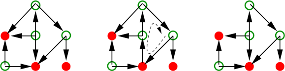
Figure 1. The first digraph is a well-colored DAG (it has several cycles, but no circuit). The second digraph is a well-colored digraph (it is not a DAG, as it contains one circuit). The third digraph is a DAG, but is not well colored (the top green vertex misses a red child). [For people who are reading a black & white version of this article, red vertices are fulfilled and green vertices are empty circles.]

4. Generating functions of well-colored unicircuit digraphs

There exists in the literature some noteworthy results on digraphs using generating functions (related e.g. to EGF of acyclic digraphs [18, 28], Cayley graphs [26], (0,1) matrices [25], Erdős–Rényi random digraph model [24]), but as fas as we know we give here the first example of application to the kernel problem.

The coloring constraints mentioned in Section 3 are “local”: they are defined only in function of each vertex and its neighbors. One nice consequence of this “local” viewpoint of kernels is that it opens up a whole range of possibilities for a kind of context-free grammar approach. Indeed if one considers rooted labeled directed trees that are well-colored (i.e. which possesses a kernel), one can describe/enumerate them with the help of the five following families of combinatorial structures (all of them being rooted labeled directed trees):

• $T$: all the trees with the coloring constraint

• ${T_{r}^{\uparrow}}$: well-colored trees with a red root (with an additional out-edge)

• ${T_{r}^{\downarrow}}$: well-colored trees with a red root (with an additional in-edge)

• ${T_{g}^{\uparrow}}$: well-colored trees with a green root (with an additional out-edge)

• ${T_{g}^{\downarrow}}$: well-colored trees with a green root (with an additional in-edge)

• ${T_{g_{r}}^{\uparrow}}$: well-colored trees with a green root (with an additional out-edge which has to be attached to a red vertex)

Those families are related by the following rules:

$$\begin{cases}T={T_{g}^{\uparrow}}\cup{T_{r}^{\uparrow}}\\ {T_{g}^{\uparrow}}=g^{\uparrow}\times{\rm Set}_{\geq 1}({T_{r}^{\uparrow}})\times{\rm Set}({T_{r}^{\downarrow}}\cup{T_{g}^{\downarrow}}\cup{T_{g}^{\uparrow}})\\ {T_{g}^{\downarrow}}=g^{\downarrow}\times{\rm Set}_{\geq 1}({T_{r}^{\uparrow}})\times{\rm Set}({T_{r}^{\downarrow}}\cup{T_{g}^{\downarrow}}\cup{T_{g}^{\uparrow}})\\ {T_{r}^{\uparrow}}=r^{\uparrow}\times{\rm Set}({T_{g}^{\downarrow}}\cup{T_{g_{r}}^{\uparrow}})\\ {T_{r}^{\downarrow}}=r^{\downarrow}\times{\rm Set}({T_{g}^{\downarrow}}\cup{T_{g_{r}}^{\uparrow}})\\ {T_{g_{r}}^{\uparrow}}=g^{\uparrow}\times{\rm Set}({T_{r}^{\uparrow}}\cup{T_{r}^{\downarrow}}\cup{T_{g}^{\downarrow}}\cup{T_{g}^{\uparrow}})\end{cases}$$

The Set operator reflects the fact that one considers non planar trees, i.e. the relative order of the subtrees attached to a given vertex does not matter. The notation ${\rm Set}_{\geq 1}$ means one considers non empty set only.

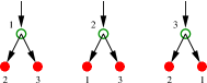
Figure 2. A tree $\in{T_{g}^{\downarrow}}$ of size 3 and all its possible labellings. ${T_{g}^{\downarrow}}$ stands for directed trees with a green root with an additional in-edge on this root.

As we are dealing with labeled objects (we refer to Figure 2 for the different labellings of a rooted directed tree), it is more convenient to use exponential generating functions, the above rules are then translated (see e.g. [20, 14] for a general presentation of this theory of “graphical enumeration/symbolic combinatorics” ) into the following set of functional equations (where $z$ marks the vertices):

$$\begin{cases}T(z)={T_{g}^{\uparrow}}(z)+{T_{r}^{\uparrow}}(z)\,,\\ {T_{g}^{\uparrow}}(z)={T_{g}^{\downarrow}}(z)=z(\exp({T_{r}^{\uparrow}}(z))-1)\exp({T_{r}^{\downarrow}}(z)+{T_{g}^{\downarrow}}(z)+{T_{g}^{\uparrow}}(z))\,,\\ {T_{r}^{\uparrow}}(z)={T_{r}^{\downarrow}}(z)=z\exp({T_{g}^{\downarrow}}(z)+{T_{g_{r}}^{\uparrow}}(z))\,.\end{cases}$$

Note that ${T_{g_{r}}^{\uparrow}}=T$ as one has the trivial bijection “${T_{g_{r}}^{\uparrow}}$ trees with a root without red child” = “${T_{r}^{\uparrow}}$ trees” and “${T_{g_{r}}^{\uparrow}}$ trees with a root with at least a red child” = “${T_{g}^{\uparrow}}$ trees”. Define now $T_{g}(z):={T_{g}^{\uparrow}}(z)$ and $T_{r}(z):={T_{r}^{\uparrow}}(z)$, the above system simplifies to:

$$\begin{cases}T(z)=T_{g}(z)+T_{r}(z)={T_{g_{r}}^{\uparrow}}(z)\,,\\ T_{g}(z)=z\exp(2T(z))-z\exp(T(z)+T_{g}(z))\,,\\ T_{r}(z)=z\exp(T_{g}(z)+T(z))=T(z)\exp(-T_{r}(z))\,.\end{cases}$$

This system has a unique solution, as the relations can be considered as fixed point equations for power series. Their Taylor expansions are:

$$T(z)=z+4\frac{z^{2}}{2!}+36\frac{z^{3}}{3!}+512\frac{z^{4}}{4!}+10000\frac{z^{5}}{5!}+248832\frac{z^{6}}{6!}+7529536\frac{z^{7}}{7!}+O(z^{8})\,,$$

$$T_{g}(z)=\quad 2\frac{z^{2}}{2!}+15\frac{z^{3}}{3!}+232\frac{z^{4}}{4!}+4535\frac{z^{5}}{5!}+114276\frac{z^{6}}{6!}+3478083\frac{z^{7}}{7!}+O(z^{8})\,,$$

$$T_{r}(z)=z+2\frac{z^{2}}{2!}+21\frac{z^{3}}{3!}+280\frac{z^{4}}{4!}+5465\frac{z^{5}}{5!}+134556\frac{z^{6}}{6!}+4051453\frac{z^{7}}{7!}+O(z^{8})\,.$$

For sure, the $i$-th coefficients of these series are divisible by $i$, as we are dealing with rooted object. Here are the 3 generating functions of the corresponding unrooted trees:

$$T^{unr.}(z)=z+2\frac{z^{2}}{2!}+12\frac{z^{3}}{3!}+128\frac{z^{4}}{4!}+2000\frac{z^{5}}{5!}+41472\frac{z^{6}}{6!}+1075648\frac{z^{7}}{7!}+O(z^{8})\,,$$

$$T_{g}^{unr.}(z)=\quad\frac{z^{2}}{2!}+5\frac{z^{3}}{3!}+58\frac{z^{4}}{4!}+907\frac{z^{5}}{5!}+19046\frac{z^{6}}{6!}+496869\frac{z^{7}}{7!}+O(z^{8})\,,$$

$$T_{r}^{unr.}(z)=z+\frac{z^{2}}{2!}+7\frac{z^{3}}{3!}+70\frac{z^{4}}{4!}+1093\frac{z^{5}}{5!}+22426\frac{z^{6}}{6!}+578779\frac{z^{7}}{7!}+O(z^{8})\,.$$

Of course, trees are DAG and therefore have a unique kernel. This implies that $T(z)$ is exactly the exponential generating function of directed rooted trees, i.e.

$$T(z)=C(2z)/2\text{ and }T_{n}=(2n)^{n-1}$$

where $C(z)$ is the Cayley function (see Figure 3 and references [5, 10]), defined by

$$C(z)=z\exp(C(z))=\sum_{n\geq 1}n^{n-1}\frac{z^{n}}{n!}\,.$$

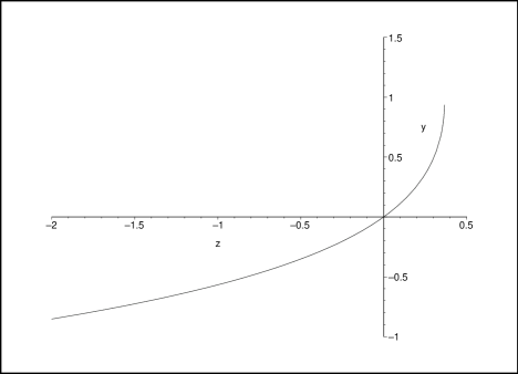
Figure 3. The Cayley tree function $C(z)$ goes from $-\infty$ for $z\sim-\infty$ to 1 at $z=\frac{1}{e}$. It satisfies $C(z)=z\exp(C(z))$.

Solving the set of equations for $T,T_{g}$ and $T_{r}$ finally leads to

Theorem 4.1 (Enumeration of well-colored trees).

By ditrees, we mean well-colored rooted labeled directed trees. By well-colored, we mean each green vertex has at least a red child, each red vertex has no red child.
The exponential generating function of ditrees is given by $T(z)=C(2z)/2$,
the EGF of ditrees with a red root is given by $T_{r}(z)=-C(-C(2z)/2)$,
the EGF of ditrees with a green root is given by $T_{g}(z)=C(2z)/2+C(-C(2z)/2)$,
where $C(z)$ is the Cayley tree function $C(z)=z\exp(C(z))$.
The EGF for the unrooted equivalent objects can be expressed in terms of the rooted ones:

$$T^{unr.}=T-T^{2}\,,\qquad T_{g}^{unr.}=T^{unr.}-T_{r}^{unr.}\,,\text{\quad and \quad}T_{r}^{unr.}=2T-2TT_{r}+T_{r}-2T/T_{r}+T_{r}^{2}/2\,.$$

Proof.

The formulae for $T,T_{r}$ and $T_{g}$ can be checked using the definition of $C(z)$ in the fix-point equations in the simplified system above. The fact that the GF for unrooted trees can be expressed in terms of the GF of rooted ones can be proven by integration of the Cayley function, or by a combinatorial splitting argument on trees. ∎

We can go on and enumerate the different possibilities of circuits for a well-colored digraph. They can be described as

$${\rm Cyc}(g)\quad\cup\quad{\rm Cyc}(r{\text{\small}\rightarrow}\{g{\text{\small}\rightarrow}\}^{+})$$

This reflects the fact that either a circuit is made up of green vertices only, or it contains some red vertices, but they have to be followed by at least a green vertex. NB: Whether one counts or not the cycles of length 1 (i.e. a single red or green vertex) will only modify the first term of the generating function. Symbolic combinatorics [14] translates the above cycle decompositions in the following function:

$$\ln\left(\frac{1}{1-g}\right)+\ln\left(\frac{1}{1-\frac{rg}{1-g}}\right)$$

where $r$/$g$ mark the number of red/green vertices. This leads to the following Theorem:

Theorem 4.2 (Enumeration of possible well-colored circuits).

The exponential generating function of possible well-colored circuits is given by

$$L(z)=-\ln(1-z-z^{2})=z+3\frac{z^{2}}{2!}+8\frac{z^{3}}{3!}+42\frac{z^{4}}{4!}+264\frac{z^{5}}{5!}+2160\frac{z^{6}}{6!}+20880\frac{z^{7}}{7!}+O(z^{8})\,.$$

Its coefficients satisfy $L_{n}=(n-1)!\,\left(\phi^{n}+\left(1-\phi\right)^{n}\right)$, where $L_{n}$ are known as the $n$-th Lucas number (usually defined by the recurrence $L_{n+2}=L_{n+1}+L_{n},L_{1}=1,L_{2}=3$) and where $\phi=(1+\sqrt{5})/2$ is the golden ratio.

Note that a reverse engineering lecture of this generating function leads to the simpler decomposition ${\rm Cyc}(g\cup rg)$, which also explains the recurrence! Now, the following decomposition of possible cycles is trivially related to the decomposition of possible circuits:

$${\rm Cyc}(r\times\{{\text{\small}\rightarrow}g\cup{\text{\small}\leftarrow}g\}^{+}\times\{{\text{\small}\rightarrow}\cup{\text{\small}\leftarrow}\})\quad\cup\quad{\rm Cyc}(g{\text{\small}\rightarrow}\cup g{\text{\small}\leftarrow})$$

leads to the EGF $-\ln(1-2z-4z^{2})$ whose coefficients are, with no surprise, $2^{n}L_{n}$.

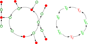
Figure 4. Unicircuit digraphs consist in a circuit with attached trees on it. The left picture above is a unicircuit digraph, to the right, we give its “canonical decomposition” as a circuit of atoms which are trees. Any well-colored unicircuit digraph has such a “canonical decomposition”.

Using the decomposition given in Figure 4, one obtains the generating function for unicircuits:

Theorem 4.3 (Enumeration of unicircuit well-colored digraphs).

The EGF of unicircuit well-colored digraphs is

$$U(z) = T^{unr.}-T_{g}+\ln\left(\frac{1}{1-(T_{g}+T_{g_{r}}T_{r})}\right)$$

$$= -\frac{C(2z)^{2}}{4}-C(-\frac{C(2z)}{2})-\ln\left(1-\frac{C(2z)}{2}-C(-\frac{C(2z)}{2})+{C\big{(}-\frac{C(2z)}{2}\big{)}\frac{C(2z)}{2}}\right)$$

$$= z+4\frac{z^{2}}{2!}+30\frac{z^{3}}{3!}+452\frac{z^{4}}{4!}+8840\frac{z^{5}}{5!}+224832\frac{z^{6}}{6!}+6909784\frac{z^{7}}{7!}+O(z^{8})\,,$$

where $C(z)$ is the Cayley tree function $C(z)=z\exp(C(z))$.

Now, consider the larger class of unicycle digraphs (digraphs which have 0 or 1 cycle). Recall that a circuit is a cycle, but a cycle is not necessarily a circuit. In order to get a “canonical decomposition” for unicyle digraphs (similar to the one given in Fig. 4 for unicircuit digraphs), one considers 3 cases:

• Either the graph has no cycle, those graphs are counted by $T^{unr.}$.

• Either it is a cycle with only $T_{g}$ trees branched on it (i.e. no red nodes in the cycle), those graphs are counted by $(\ln\left(\frac{1}{1-2T_{g}}\right)-2Tg-4Tg^{2}/2)/2+Tg^{2}/2$, where $2Tg$ corresponds to $T_{g}\times\{\rightarrow\cup\leftarrow\}$, one removes cycles of length 1 and 2 from the logarithm (this explains the $-2Tg-4Tg^{2}/2$ term) and one divides the whole formula by 2 because one has to take into account the fact the cycle can be read clockwise or not, and one adds the only legal cycle of length 2.

• Either the graph contains a cycle with some red nodes and then one considers the following possible “bricks”:

  $$\begin{cases}T_{r}\leftarrow T_{g_{r}}\leftarrow\\ T_{r}\leftarrow T_{g_{r}}\rightarrow\qquad\text{(but not a cycle of length 2, because multiarcs are not allowed) }\\ T_{r}\rightarrow\left(T_{g}\{\rightarrow\cup\leftarrow\}\right)^{*}T_{g}\leftarrow\qquad\text{(but not a cycle of length 2)}\\ T_{r}\rightarrow\left(T_{g}\{\rightarrow\cup\leftarrow\}\right)^{*}T_{g_{r}}\rightarrow\\ T_{r}\leftarrow T_{g_{r}}\{\rightarrow\cup\leftarrow\}\left(T_{g}\{\rightarrow\cup\leftarrow\}\right)^{*}T_{g}\leftarrow\\ T_{r}\leftarrow T_{g_{r}}\{\rightarrow\cup\leftarrow\}\left(T_{g}\{\rightarrow\cup\leftarrow\}\right)^{*}T_{g_{r}}\rightarrow\end{cases}$$

Theorem 4.4 (Enumeration of unicycle well-colored digraphs).

The EGF of unicycle well-colored digraphs is

$$V(z) = T^{unr.}+\frac{1}{2}\ln\left(\frac{1}{1-2T_{g}}\right)-Tg-Tg^{2}/2-TrTg/2-T_{r}T/2$$

$$+\frac{1}{2}\ln\left(\frac{1}{1-\left(2T_{r}T_{g_{r}}+\frac{T_{r}T_{g}+T_{r}T_{g_{r}}+2T_{r}T_{g_{r}}T_{g}+2T_{r}T_{g_{r}}^{2}}{1-2T_{g}}\right)}\right)$$

$$= T^{unr.}-T+T_{r}-T^{2}/2-\ln(1+T_{r})-\frac{1}{2}\ln(1-2T)$$

$$= z+4\frac{z^{2}}{2!}+36\frac{z^{3}}{3!}+692\frac{z^{4}}{4!}+15920\frac{z^{5}}{5!}+458622\frac{z^{6}}{6!}+15559264\frac{z^{7}}{7!}+O(z^{8})\,.$$

where $T$, $T_{g}$, $T_{r}$, and $T^{unr.}$ are given in Theorem 4.1.

Note that in the two theorems above, any given non-colored graph is counted with multiplicity 0, 1 or 2 (if there are 0, 1 or 2 ways to color it). We explained in Section 3 that a multiplicity larger than 2 was not possible for unicycle digraphs. We enumerate in the following proposition those with exactly 2 possible colorations.

Proposition 4.5 (Enumeration of unicycle digraphs with two kernels).

The EGF of unicycle digraphs with 2 kernels is

$$D(z)=-\ln\sqrt{1+C(-C(2z)/2)^{2}}\,,$$

where $C(z)$ is the Cayley tree function $C(z)=z\exp(C(z))$.

Remark: From the definition of cycle/circuit, $D(z)$ is also the EGF of unicircuit digraphs with 2 kernels.

Proof.

Let $\mathcal{D}$ be the set of unicycle digraphs with 2 kernels. First, it is easy to see that ${\rm Cyc}(T_{r}^{2})\subset\mathcal{D}$ (with a sligth abuse of notation, as we first only consider the shape, not the coloration of the $T_{r}$ trees): simply color the nodes in the cycle alternatively in green and red, and switch the colors of a part of attached trees, if needs be.

We now prove the next step $\mathcal{D}\subset{\rm Cyc}(T_{r}^{2})$: Take a unicycle graph in $\mathcal{D}$, it means at least one of its vertex can be colored both green and red. Such a vertex $v$ can be taken, without loss of generality, in the circuit (from the above remark, the cycle is in fact a circuit). [If it were not the case, all bi-colorabled vertices would be in the tree components, but then one could split our graph to get DAGs which are known to be uniquely colorable]. But when $v$ is red, it implies it has only $T_{g}$ trees attached to it, which means than when it gets green, the next node in the circuit has be red (and was previously green!). This implies alternation red/green (and even length for parity reasons) for all the nodes in the circuit.

This leads to a canonical decomposition

$${\rm Cyc}(T_{r}^{2})\,.$$

If one divides by 2 for the (anti)clockwise readings, this leads to the Theorem. ∎

Most of these results (and also the computations of Section 5 hereafter) were checked with the computer algebra system Maple. A worksheet corresponding to this article is available at http://algo.inria.fr/banderier/Paper/kernels.mws (or kernels.html), it uses the Algolib librairy, downloadable at http://algo.inria.fr/libraries/).

5. Asymptotics

In this section, we give asymptotic results for $n\rightarrow+\infty$.

Theorem 5.1 (Proportion of trees with a green/red root).

Asymptotically $\frac{1-\lambda}{1+\lambda}\approx 47.95\%$ of the trees have a green root, where the constant $\lambda\approx 0.351733$ is defined as the unique real root of $2\lambda=\exp(-\lambda)$.

A more pleasant way to formulate this Theorem consists in considering Nim-type games (first player who cannot move loses) on directed trees where the tree and the starting position are chosen uniformly at random. The strategies of the two players being optimal, the first player has then a probability of 47.95% (asymptotically) to win the game. (Recall that if the starting position can be chosen by the first player, then he will always win.)

Proof.

The key step of this result and the following ones are the following expansions (derived from the expansion of the Cayley function) for $T$, $T_{r}$ and $T_{g}$:

$$T(z)\sim\frac{5}{6}-\frac{1}{\sqrt{2}}\sqrt{1-2ez}+O(1-2ez)$$

$$T_{r}(z)\sim\lambda-\frac{\lambda\sqrt{2}}{1+\lambda}\sqrt{1-2ez}+O(1-2ez)$$

$$T_{g}(z)\sim\frac{1}{2}-\lambda-\frac{1}{\sqrt{2}}\frac{1-\lambda}{1+\lambda}\sqrt{1-2ez}+O(1-2ez)\,,$$

where the constant $\lambda$ is defined as $\lambda:=T_{r}(\frac{1}{2e})\approx 0.351733$.

By Pringsheim theorem [14], as $T_{r}(z)$ has nonnegative coefficients, then $T_{r}(z)$ has a positive singularity. As coefficients of $T_{r}$ are smaller than coefficients of $T$, its radius of convergence belongs to $[0,1/(2e)]$. Now, $-C(2z)/2$ is negative on this interval, and thus $C(-C(2z)/2)$ is analytic there, and $1/(2e)$ is therefore its only possible dominating singularity. The radius of $T_{g}$ follows from $T=T_{r}+T_{g}$. The theorem follows by considering $\frac{[z^{n}]T_{g}(z)}{[z^{n}]T(z)}=\frac{1-\lambda}{1+\lambda}-\frac{\lambda^{2}(\lambda+4)}{(1+\lambda)^{5}}\frac{1}{n}+O(\frac{1}{n^{2}})$. ∎

Theorem 5.2 (Proportion of red vertices in possible circuits).

Asymptotically $\frac{1}{2}-\frac{1}{2\sqrt{5}}\approx 27.63\%$ of the vertices of a possible circuits are red.

Proof.

One has to considerer the following bivariate generating function (exponential in $z$, ordinary in $u$): $\ln\left(\frac{1}{1-(z+uz^{2})}\right)$. The wanted proportion is then given by $\frac{[z^{n}]\partial_{u}F(z,1)}{[z^{n}]F(z,1)}$, where [$z^{n}]\partial_{u}F(z,1)$ means the $n$-th coefficient of “the derivative with respect to $u$ of $F(z,u)$, then evaluated at $u=1$”. ∎

Then, one can wonder if the asymptotic density of well-colored unicircuit graphs is more than 50% or even if it is 100%? The following theorem gives the answer:

Theorem 5.3 (Proportion of well-colored unicircuit digraphs).

The proportion of well-colored graphs amongst unicircuit digraphs is asymptotically:

$$\frac{3\lambda^{3}+\lambda^{2}-\lambda-1}{(1+\lambda)^{2}(\lambda-1))}\approx 92.65\%$$

where $\lambda$ is the constant defined in Theorem 5.1.

Proof.

Relies on a singularity analysis of the generating function of Theorem 4.3, with the expansions given in Theorem 5.1. Note that some unicircuit digraphs can have 2 kernels, so one has to perform the following asymptotic expansions:

$$\frac{[z^{n}]U(z)-D(z)}{[z^{n}]F(z)}\approx 92.65-\frac{0.12}{n}+O(\frac{1}{n^{2}})\,,$$

where $F(z)=T^{unr}(z)+\ln(\frac{1}{1-T(z)})-T(z)$ is the EGF of (non-colored) unicircuit digraphs. ∎

For sure, it one considers now the asymptotic density of well-colored unicircuit graphs, the proportion should be larger, as one only adds DAGs (which are all well-colorable). The following theorem gives the noteworthy result that unicircuit graphs are in fact almost surely well-colored:

Theorem 5.4 (Proportion of well-colored unicycle digraphs).

There is asymptotically a proportion of $1-\frac{2\lambda^{3}\sqrt{2}}{(1+\lambda)^{2}(1-\lambda)\sqrt{\pi}}\frac{1}{\sqrt{n}}\approx 1-\frac{0.05}{\sqrt{n}}$ of well-colored graphs amongst unicycle digraphs of size $n$, where $\lambda$ is the constant defined in Theorem 5.1.

Proof.

Relies on a singularity analysis of the generating function of Theorem 4.4, with the expansions given in Theorem 5.1. Note that some unicycle digraphs can have 2 kernels, so one has to consider

$$\frac{[z^{n}]V(z)-D(z)}{[z^{n}]G(z)}\,,$$

where $G(z)=T^{unr}(z)+\frac{1}{2}\ln(\frac{1}{1-2T(z)})-T(z)-T(z)^{2}/2$ is the EGF of (non-colored) unicycle digraphs (one substracts $T^{2}/2$ because amongst the 4 graphs with a cycle of length 2 created by the $\ln(\frac{1}{1-2T(z)})$ part, 3 are not legal: 1 was already counted because of symmetries, and the other 2 have in fact a multiple arc, whereas it is forbidden for our digraphs). ∎

Finally, if one considers graphs with at most $k$ cycles, it means one has more cutting points, which relaxes the constraints for well-colarability (=existence of kernel). According to the above results, this implies an asymptotic density of one. This gives as a corolary of our results, that all these families have almost surely a kernel. A kind of “limit case” is dense graphs, for which some results already mentionned by Fernandez de la Vega [13] and Tomescu [30] give that they have indeed almost surely a kernel.

6. Conclusion

It is quite pleasant that our generating function approach allows to get new results on the kernel problem, giving e.g. the proportion of graphs satisfying a given property, and new informations on Nim-type games for some families of graphs.

As a first extension of our work, it is possible to apply classical techniques from analytic combinatorics [14] in order to get informations on standard deviation, higher moments, and limit laws for statistics studied in Section 5.

Another extension is to get closed form formulas for bicircuit/bicycles digraphs, (the generating function involves the derivative of the product of two logs and the asymptotics are performed like in our Section 5). It is still possible (for sure with the help of a computer algebra system) to do it for 3 or 4 cycles but the “canonical decompositions” and the computations get cumbersome. In order to go on our analysis far beyond low-cyclic graphs, one needs an equation similar to the one given by E.M. Wright [32, 33] for graphs. Let $\mathcal{W}_{\ell}$ be the family of well-colored digraphs with $\ell$ edges more than vertices, ($\ell\geq-1$). It is possible to get an equation “à la Wright” for $\mathcal{W}_{\ell}$ by pointing any edge (except edges linking a green vertex to a red one) in a well-colored digraph. It is however not clear for yet if and how such equations can be simplified in order to get a recurrence as “simple/nice” to the one that Wright got for graphs, thus opening the door to asymptotics and threshold analysis beyond the unicyclic case.

Acknowledgements. This work was partially realized while the second author (Jean-Marie Le Bars) benefited from a delegation CNRS in the Laboratoire d’Informatique de Paris Nord (LIPN). We would like to thank Guy Chaty and François Lévy for a friendly discussion and their bibliographical references [7, 29]. We also thank an anomymous referee for detailed comments on a somehow preliminary version of this work.

References

- [1] C. Berge and P. Duchet. Recent problems and results about kernels in directed graphs. In Applications of discrete mathematics (Clemson, SC, 1986), pages 200–204. SIAM, Philadelphia, PA, 1988.
- [2] Claude Berge. Graphs, volume 6 of North-Holland Mathematical Library. North-Holland Publishing Co., Amsterdam, 1985. Second revised edition of part 1 of the 1973 English version.
- [3] Claude Berge and Marcel Paul Schützenberger. Jeux de Nim et solutions. C. R. Acad. Sci. Paris, 242:1672–1674, 1956.
- [4] Immanuel M. Bomze, Marco Budinich, Panos M. Pardalos, and Marcello Pelillo. The maximum clique problem. In Handbook of combinatorial optimization, Supplement Vol. A, pages 1–74. Kluwer Acad. Publ., Dordrecht, 1999.
- [5] A. Cayley. A theorem on trees. Quart. J., XXIII:376–378, 1889.
- [6] Claudette Cayrol, Sylvie Doutre, and Jérôme Mengin. On decision problems related to the preferred semantics for argumentation frameworks. Journal of Logic and Computation, 13(3):377–403, 2003.
- [7] Guy Chaty, Y. Dimopoulos, V. Magirou, C.H. Papadimitriou, and Jayme L. Szwarcfiter. Enumerating the kernels of a directed graphs with no odd circuits (erratum). Information Processing Letters, To appear, 2003.
- [8] Guy Chaty and François Lévy. Default logic and kernels in digraphs. Université de Paris-Nord, Villetaneuse, Rapport LIPN 91-9, 1991.
- [9] V. Chvátal. On the computational complexity of finding a kernel. Technical report, Report NO CRM-300, univ. de Montréal, Centre de Recherches Mathématiques, 1973.
- [10] Robert M. Corless, David J. Jeffrey, and Donald E. Knuth. A sequence of series for the Lambert function. In Proceedings of the 1997 International Symposium on Symbolic and Algebraic Computation (Kihei, HI), pages 197–204 (electronic), New York, 1997. ACM.
- [11] Nadia Creignou. The class of problems that are linearly equivalent to satisfiability or a uniform method for proving NP-completeness. Theoretical Computer Science, 145(1-2):111–145, 1995.
- [12] Sylvie Doutre. Autour de la sémantique préférée des systèmes d’argumentation. PhD thesis, Université Paul Sabatier, Toulouse, 2002. Thèse de Doctorat.
- [13] W. Fernandez de la Vega. Kernels in random graphs. Discrete Mathematics, 82(2):213–217, 1990.
- [14] Philippe Flajolet and Robert Sedgewick. Symbolic and Analytic Combinatorics. To appear (chapters are avalaible as Inria research reports). See http://algo.inria.fr/flajolet/Publications/books.html, 2003.
- [15] Aviezri S. Fraenkel. Planar kernel and Grundy with , , are NP-complete. Discrete Applied Mathematics, 3(4):257–262, 1981.
- [16] Aviezri S. Fraenkel. Combinatorial game theory foundations applied to digraph kernels. Electronic Journal of Combinatorics, 4(2):Research Paper 10, approx. 17 pp. (electronic), 1997. The Wilf Festschrift (Philadelphia, PA, 1996).
- [17] Masahiko Fukuyama. A Nim game played on graphs. Theoretical Computer Science, 304(1-3):387–419, 2003.
- [18] Ira M. Gessel. Counting acyclic digraphs by sources and sinks. Discrete Mathematics, 160(1-3):253–258, 1996.
- [19] Valentin Goranko and Bruce Kapron. The modal logic of the countable random frame. Archive for Mathematical Logic, 42(3):221–243, 2003.
- [20] Frank Harary and Edgar M. Palmer. Graphical enumeration. Academic Press, New York, 1973.
- [21] Jean-Marie Le Bars. Fragments of existential second-order logic without - laws. In Thirteenth Annual IEEE Symposium on Logic in Computer Science (Indianapolis, IN, 1998), pages 525–536. IEEE Computer Soc., Los Alamitos, CA, 1998.
- [22] Jean-Marie Le Bars. Counterexamples of the 0-1 law for fragments of existential second-order logic: an overview. The Bulletin of Symbolic Logic, 6(1):67–82, 2000.
- [23] Jean-Marie Le Bars. The 0-1 law fails for frame satisfiability of propositional modal logic. In Proceedings of the 17th IEEE Symposium on Logic in Computer Science. 2002.
- [24] Tomasz Łuczak. Phase transition phenomena in random discrete structures. Discrete Mathematics, 136(1-3):225–242, 1994. Trends in discrete mathematics.
- [25] B. D. McKay, G. F. Royle, I. M. Wanless, F. E. Oggier, N. J. A. Sloane, and H. Wilf. Acyclic digraphs and eigenvalues of (0,1)-matrices. Preprint, 2003.
- [26] Marni Mishna. Attribute grammars and automatic complexity analysis. Advances in Applied Mathematics, 30(1-2):189–207, 2003. Formal power series and algebraic combinatorics (Scottsdale, AZ, 2001).
- [27] Moses Richardson. Solutions of irreflexive relations. Ann. of Math. (2), 58:573–590, 1953. (Errata in vol. 60, p. 595, 1954).
- [28] Robert W. Robinson. Counting labeled acyclic digraphs. In New directions in the theory of graphs (Proc. Third Ann Arbor Conf., Univ. Michigan, Ann Arbor, Mich., 1971), pages 239–273. Academic Press, New York, 1973.
- [29] Jayme L. Szwarcfiter and Guy Chaty. Enumerating the kernels of a directed graph with no odd circuits. Information Processing Letters, 51(3):149–153, 1994.
- [30] Ioan Tomescu. Almost all digraphs have a kernel. In Random graphs ’87 (Poznań, 1987), pages 325–340. Wiley, Chichester, 1990.
- [31] John von Neumann and Oskar Morgenstern. Theory of games and economic behavior. Princeton University Press, Princeton, N.J., third edition, 1980.
- [32] E. M. Wright. The number of connected sparsely edged graphs. J. Graph Theory, 1(4):317–330, 1977.
- [33] E. M. Wright. The number of connected sparsely edged graphs. III. Asymptotic results. Journal of Graph Theory, 4(4):393–407, 1980.