Hyperbolic 3-manifolds with geodesic boundary:
Enumeration and volume calculation

Abstract

We describe a natural strategy to enumerate compact hyperbolic $3$-manifolds with geodesic boundary in increasing order of complexity. We show that the same strategy can be employed to analyze simultaneously compact manifolds and finite-volume manifolds having toric cusps. In opposition to this we show that, if one allows annular cusps, the number of manifolds grows very rapidly, and that our strategy cannot be employed to obtain a complete list. We also carefully describe how to compute the volume of our manifolds, discussing formulae for the volume of a tetrahedron with generic dihedral angles in hyperbolic space.

MSC (2000): 57M50.

According to Thurston’s geometrization program, the theory of hyperbolic manifolds plays a central role in $3$-dimensional topology. Hyperbolic manifolds with geodesic boundary, the first example of which was given by Thurston himself in [48] (and later generalized in [41]), are an important portion of this theory. On the other hand, the algorithmic and computer approach to $3$-manifolds has been acquiring an increasing popularity in recent years. For cusped hyperbolic manifolds this approach, which was worked out in [5, 45, 54, 55] and several other papers, again depends on ideas of Thurston, namely on the use of moduli for hyperbolic ideal tetrahedra and equations to ensure consistency of the structures. For closed manifolds the basics of the computer approach were set by Matveev in [35] (see also [14, 36]), and several experimental results were later obtained by himself and other authors (see [32, 33]). In the present paper we describe the general setting of the algorithmic approach to hyperbolic $3$-manifolds with geodesic boundary, concentrating in particular on their enumeration in order of increasing complexity, and on the computation of their volume.

1 Hyperbolic structures

In this section we review the general theory of hyperbolic $3$-manifolds with geodesic boundary, stating the main results we will need in the sequel.

Local structure, cusps, compactifications

In the rest of this paper we will call hyperbolic an orientable finite-volume complete Riemannian $3$-manifold with non-empty boundary, locally isometric to an open subset of a closed half-space of $\mathbb{H}^{3}$. We will always denote such a manifold by $Y$. Note that $\partial Y$ is totally geodesic. Doubling $Y$ along its boundary and using the description of the ends of the double [3], one can show that $Y$ consists of a compact portion together with some “toric and annular cusps.” A toric cusp is here a space of the form $T\times[0,\infty)$, attached to the rest of $Y$ along $T\times\{0\}$, and an annular cusp is defined analogously. Note that toric cusps are disjoint from $\partial Y$, while an annular cusp gives two punctures in $\partial Y$. In particular, $\partial Y$ is compact if and only if $Y$ has no annular cusps.

Given $Y$ as above, we can naturally get a compact manifold $\overline{Y}$ by adding a torus $T\times\{\infty\}$ for each toric cusp $T\times[0,\infty)$, and an annulus $A\times\{\infty\}$ for each annular cusp $A\times[0,\infty)$. However, it turns out that when there are annular cusps another compactification $\overline{\overline{Y}}$ of $Y$ is more suited to the geometric situation. We define $\overline{\overline{Y}}$ as a quotient of $\overline{Y}$, where in each annular cusp $A\times[0,\infty]$ with $A=S^{1}\times[0,1]$, for all $t\in[0,1]$ we collapse $S^{1}\times\{t\}\times\{\infty\}$ to one point $\{*\}\times\{t\}\times\{\infty\}$. Note that $Y$ is obtained from $\overline{\overline{Y}}$ by removing some toric boundary components and drilling some properly embedded arcs.

Rigidity and Kojima decomposition

A key result for computational purposes is the following:

Theorem 1.1.

Any two homeomorphic hyperbolic manifolds are isometric.

This result is commonly referred to as rigidity theorem, and a proof for the geodesic boundary case was spelled out in [18].

Another very important fact is that the hyperbolic structure determines certain combinatorial data which can be employed to efficiently test two manifolds for homeomorphism. This result is analogous to the Epstein-Penner decomposition of cusped hyperbolic manifolds without boundary [13], and it was proved by Kojima [27, 28]. Its statement involves the notion of truncated polyhedron, that we now give. Consider the projective model of hyperbolic $3$-space, viewed as the open unit ball $\mathbb{B}^{3}$ in the Euclidean $3$-space $\mathbb{E}^{3}$. Let us call finite the points of $\mathbb{B}^{3}$, ideal those of $\partial\mathbb{B}^{3}$, and ultra-ideal the other points of $\mathbb{E}^{3}$. Consider a convex polyhedron $\widetilde{P}$ in $\mathbb{E}^{3}$ with ideal and/or ultra-ideal vertices, and all edges meeting the closure of $\mathbb{B}^{3}$. Dual to each ultra-ideal vertex of $\widetilde{P}$ there is an open hyperbolic half-space, and we define $P$ to be $\widetilde{P}\cap\mathbb{B}^{3}$ minus these half-spaces. Any $P$ arising like this from some $\widetilde{P}$ will be called a truncated polyhedron. Note that $P$ has internal faces, those coming from faces of $\widetilde{P}$, and truncation faces. Moreover internal and truncation faces lie at right angles to each other.

Theorem 1.2.

Any hyperbolic manifold admits a canonical decomposition as a gluing of truncated polyhedra along the internal faces.

In the sequel we will need to refer to the geometric argument underlying this result, so we briefly sketch it here. Regard $\mathbb{E}^{3}$ as the hyperplane at height $1$ in Minkowsky $4$-space $\mathbb{M}^{\,3,1}$. Suppose first that $Y$ has no toric cusps, and identify the universal cover of $Y$ to an intersection of half-spaces of $\mathbb{B}^{3}$. Dual to each such subspace there is a point having norm $1$ in $\mathbb{M}^{\,3,1}$, and the decomposition of $Y$ is obtained by taking the faces of the convex hull of all these points, projecting first to $\mathbb{E}^{3}$, truncating, and then projecting to $Y$. When there are toric cusps one must also take suitably small Margulis neighbourhoods of these cusps, lift them to horoballs in $\mathbb{B}^{3}$, consider the duals to these horoballs on the light-cone of $\mathbb{M}^{\,3,1}$, include these duals in the convex hull, and suitably subdivide some of the resulting faces. We address the reader to [18] for all the details.

We are now in a position to explain why we have introduced the compactification $\overline{\overline{Y}}$:

Proposition 1.3.

Let $Y$ be hyperbolic. For each truncated polyhedron $P$ in the Kojima decomposition of $Y$, consider the corresponding Euclidean polyhedron $\widetilde{P}$. Glue these $\widetilde{P}$’s along the same maps as in the Kojima decomposition, and remove open stars of the vertices. The resulting space is then homeomorphic to $\overline{\overline{Y}}$.

Topological obstructions to hyperbolicity

Since dealing with open manifolds is impossible by computer, the idea to enumerate the hyperbolic $Y$’s is to enumerate the corresponding compact $\overline{Y}$’s or $\overline{\overline{Y}}$’s. The next two results show that the presence of annular cusps makes a dramatic difference. The former can be found in [18], the latter follows from the results discussed in Section 6. (Recall that we are calling ‘hyperbolic’ a manifold with non-empty geodesic boundary).

Theorem 1.4.

Let $M$ be a compact orientable $3$-manifold with boundary, and let $Y$ be $M$ minus the toric components of $\partial M$. The following conditions are pairwise equivalent:

• $Y$ is hyperbolic;

• $Y$ is hyperbolic, it has no annular cusps, and $\overline{Y}\cong M$;

• $M$ is irreducible, boundary-irreducible, acylindrical and atoroidal, and $\chi(M)<0$.

Proposition 1.5.

• For any $g\geqslant 2$ there exists a hyperbolic $Y$ such that $\overline{Y}$ is the handlebody of genus $g$;

• For any compact $3$-manifold $M$ there exists a hyperbolic $Y$ such that $\overline{\overline{Y}}\cong M$.

2 Complexity of 3-manifolds
and enumeration strategy

In this section we recall the basics of the theory of simple and special spines, and the related theory of ideal triangulations, describing how it can be employed to (partially) enumerate the class of $3$-manifolds we are interested in. Proofs of all results on spines and complexity can be found in [36].

Simple spines and complexity

Throughout the present section we will employ the PL category for $3$-manifolds and use the customary notions of PL topology, see [43]. A simple polyhedron is a compact polyhedron $P$ such that the link of each point of $P$ can be embedded in the space given by a circle with three radii. In particular, $P$ has dimension at most $2$. Finite graphs and closed surfaces are examples of simple polyhedra. A point of a simple polyhedron is called a vertex if its link is precisely given by a circle with three radii. A regular neighbourhood of a vertex is shown in Fig. 1-(3).

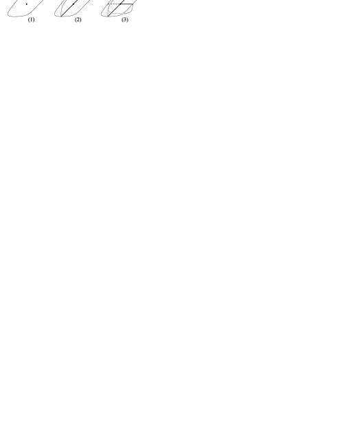
Figure 1: Local aspect of an almost-special polyhedron.

From the figure one sees that the vertices are isolated, whence finite in number. Graphs and surfaces do not contain vertices.

If $M$ is a compact $3$-manifold with non-empty boundary, we call spine of $M$ a subpolyhedron $P$ of $M$ such that $M\setminus P$ is an open collar of $\partial M$. We call complexity of $M$, and denote by $c(M)$, the minimal number of vertices of a simple spine of $M$. We say that a spine of $M$ is minimal if it has $c(M)$ vertices and it does not contain any proper subpolyhedron which is also a spine of $M$.

Special spines and ideal triangulations

We now introduce a more restrictive type of spine which turns out to have a very clear geometric counterpart. A simple polyhedron $P$ is called almost-special if the link of each point of $P$ is given by a circle with either zero, or two, or three radii. The local aspects of $P$ are correspondingly shown in Fig. 1. The points of type (2) or (3) are called singular, and the set of singular points of $P$ is denoted by $S(P)$. We will say that $P$ is special if it is almost-special, $S(P)$ contains no circle component, and $P\setminus S(P)$ consists of open $2$-discs.

We now call ideal triangulation of a compact $3$-manifold $M$ with non-empty boundary a realization of the interior of $M$ as follows. We take a finite number of tetrahedra, we glue together in pairs the faces of these tetrahedra along simplicial maps, and we remove the vertices. Equivalently, an ideal triangulation of $M$ is a realization of $M$ as a gluing of truncated tetrahedra. The relation between spines and triangulations is given by the following:

Proposition 2.1.

The set of ideal triangulations of a $3$-manifold $M$ corresponds bijectively to the set of special spines of $M$. The polyhedron corresponding to a triangulation is the $2$-skeleton of the dual cellularization, as shown in Fig. 2.

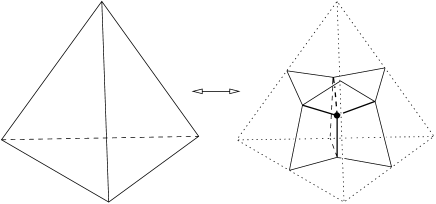
Figure 2: Duality between triangulations and special polyhedra.

Manifolds having special minimal spines

Special spines have two main advantages if compared to merely simple ones. First of all, a special spine determines the manifold it is a spine of [6], which is false for simple spines. Second, no efficient method for listing simple spines is known, whereas enumerating special spines in increasing order of complexity is very easy (at least theoretically, see [4]). For these reasons, the next result is crucial for computational purposes:

Proposition 2.2.

Let $M$ be a compact $3$-manifold with non-empty boundary. The following conditions are pairwise equivalent:

• $M$ is irreducible, $\partial$-irreducible, acylindrical, and not the $3$-disc;

• $M$ has some special minimal spine;

• All minimal spines of $M$ are special.

This result is not quite stated in this form in [36] or in any of Matveev’s papers, but it easily follows from the proof of [36, Theorem 2.2.4].

Naïf enumeration strategy

Cusped hyperbolic manifolds without boundary were studied and enumerated in [5], which explains why we have decided to restrict to manifolds with non-empty boundary. In addition, we forbid here the presence of annular cusps, because, according to Propositions 1.5 and 2.2, the theory of spines, triangulations, and complexity does not appear to be well-suited for the investigation of such manifolds. See Section 6.

Let us then define $\mathcal{H}_{n}$ as the set of all hyperbolic manifolds having complexity $n$ and non-empty compact geodesic boundary. We also define $\widetilde{\mathcal{H}}_{n}$ as the set of all orientable, compact, irreducible, $\partial$-irreducible, and acylindrical manifolds with negative $\chi$. Theorem 1.4 implies that if $Y\in\mathcal{H}_{n}$ then $\overline{Y}\in\widetilde{\mathcal{H}}_{n}$. Conversely, if $M\in\widetilde{\mathcal{H}}_{n}$, then $M$ minus the toric components of $\partial M$ belongs to $\mathcal{H}_{n}$ if and only if $M$ is atoroidal. We can then view $\widetilde{\mathcal{H}}_{n}$ as the set of candidate hyperbolic manifolds with complexity $n$ and without annular cusps.

Note now that Proposition 2.2 applies to the elements of $\widetilde{\mathcal{H}}_{n}$. Therefore the following theoretical steps lead to the exact determination of $\mathcal{H}_{n}$, assuming $\mathcal{H}_{m}$ is known inductively for $m<n$:

1. Produce the list of all special spines with $n$ vertices and negative $\chi$;

2. Remove from the list the spines $P$ whose associated manifold $M(P)$ is not hyperbolic;

3. Remove from the list the spines $P$ such that $M(P)$ belongs to some $\mathcal{H}_{m}$ for $m<n$;

4. For $P$ varying in the list, compare the manifolds $M(P)$ for equality, discarding duplicates.

Step (1) does not present any theoretical difficulty, but its practical implementation is quite demanding if no computational shortcuts are employed. We will discuss these shortcuts in the next paragraph. And we will explain how to carry out the other steps in the next section.

Pseudo-minimal spines

Taking into account Propositions 2.1 and 2.2, the reader may wonder why we have employed special spines rather than triangulations to list the elements of $\mathcal{H}_{n}$. The first remark is that one can always restrict to minimal triangulations without losing any potentially interesting manifold. However, it turns out that dual to a triangulation which is minimal among triangulations of the same manifold, there is often a special spine which is not minimal among simple spines of the same manifold. Of course this can only happen if the corresponding manifold violates one of the topological constraints of Proposition 2.2, but we know from Theorem 1.4 that in this case the manifold is not hyperbolic, so we can discard it. In other words, non-minimality is a much more flexible notion for spines than for triangulations, so using spines we can substantially reduce the list of manifolds that we will later need to investigate.

Of course it is impossible to check in a direct fashion whether a special spine is minimal, but there are many criteria for non-minimality, which can be used as tests to discard spines which will certainly not bring any relevant manifold. The tests used in [17] are based on the moves shown in Fig. 3, which are easily seen to transform a spine

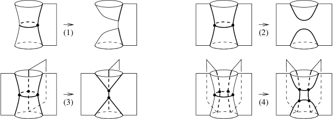
Figure 3: Moves on simple spines.

of a manifold into another spine of the same manifold. To be precise, let us say that a spine is pseudo-minimal if it cannot be transformed into a spine with fewer vertices by a combination of the moves shown in Fig. 3. The key point mentioned above on the flexibility of spines is that moves (1) and (2) do not lead to special spines (in general), so they do not have counterparts at the level of triangulations. The first step of the enumeration strategy is then replaced by the following:

• Produce the list of all pseudo-minimal special spines with $n$ vertices and negative $\chi$.

We also mention that another trick very important for computational purposes is to construct the candidate spines portion after portion, following the branches of a tree, and to apply the non-minimality tests arising from the moves of Fig. 3 also to partially constructed spines, thus “cutting the dead branches” at their bases.

3 Hyperbolicity equations and tilts

In this section we discuss how an ideal triangulation can be employed to construct a hyperbolic structure on a given manifold and to recognize the canonical Kojima decomposition of that manifold. This allows to carry out steps (2)-(4) of the enumeration strategy for $\mathcal{H}_{n}$ explained in the previous section. We actually include in the discussion also manifolds with annular cusps, because the methods via ideal triangulations to construct and recognize the hyperbolic structure apply to these manifolds too. It is only step (1) of the enumeration strategy (the listing of special spines) that is not suited to manifolds with annular cusps, and the reason why these manifold are ruled out from $\mathcal{H}_{n}$.

We first treat the compact case and then sketch the variations needed for the case where there are also some cusps. For all details and proofs (and for some very natural terminology that we use here without giving actual definitions) we address the reader to [18].

Compact case: moduli and equations

The basic idea for constructing a hyperbolic structure via an ideal triangulation is to realize the tetrahedra of the triangulation as truncated tetrahedra in $\mathbb{H}^{3}$ and then require that the structures match when the tetrahedra are glued together. The following facts show that one can use the dihedral angles as moduli to parameterize the realizations of a tetrahedron and to check consistency:

• A hyperbolic structure on a combinatorial truncated tetrahedron is determined by the 6-tuple of dihedral angles along the internal edges;

• The only restriction on this 6-tuple of positive reals is that the angles of each of the four truncation triangles should sum up to less than $\pi$;

• The lengths of the internal edges can be computed as explicit functions of the dihedral angles;

• A choice of hyperbolic structures on the tetrahedra of an ideal triangulation of a manifold $M$ gives rise to a hyperbolic structure on $M$ if and only if all matching edges have the same length and the total dihedral angle around each edge of $M$ is $2\pi$.

Given an ideal triangulation consisting of $n$ tetrahedra one then has the hyperbolicity equations: a system of $6n$ equations with unknown varying in an open set of $\mathbb{R}^{6n}$ which, by rigidity (Theorem 1.1), admits one solution at most.

Canonical decomposition and tilts

Once a hyperbolic structure has been constructed on a manifold $Y$ using an ideal triangulation $\mathcal{T}$, one natural issue is to decide if $\mathcal{T}$ is the canonical decomposition of $Y$ and, if not, to promote $\mathcal{T}$ to become canonical. These matters are faced using the tilt formula [50, 51, 54], that we now describe.

Recall first that the Kojima decomposition of $Y$ is constructed by projecting first to $\mathbb{H}^{3}$ and then to $Y$ the faces of the convex hull of the set $\mathcal{P}\subset\mathbb{M}^{\,3,1}$ of the duals to the boundary components of the universal cover of $Y$. If $\sigma$ is a $d$-simplex in $\mathcal{T}$, each end of a lifting of $\sigma$ to $\mathbb{H}^{3}$ determines a point of $\mathcal{P}$. Now let two tetrahedra $\Delta_{1}$ and $\Delta_{2}$ share a $2$-face $F$, and let $\widetilde{\Delta}_{1},\widetilde{\Delta}_{2}$ and $\widetilde{F}$ be liftings of $\Delta_{1},\Delta_{2}$ and $F$ to $\mathbb{H}^{3}$ such that $\widetilde{\Delta}_{1}\cap\widetilde{\Delta}_{2}=\widetilde{F}$. Let $\overline{F}$ be the $2$-subspace of $\mathbb{M}^{\,3,1}$ that contains the three points of $\mathcal{P}$ determined by $\widetilde{F}$. For $i=1,2$ let $\overline{\Delta}^{(F)}_{i}$ be the half-$3$-subspace bounded by $\overline{F}$ and containing the fourth point of $\mathcal{P}$ determined by $\widetilde{\Delta}_{i}$. Then one can show that $\mathcal{T}$ is the canonical Kojima decomposition of $Y$ if and only if, whatever $F,\Delta_{1},\Delta_{2}$, the following conditions are met:

• the convex hull of $\overline{\Delta}^{(F)}_{1}$ and $\overline{\Delta}^{(F)}_{2}$ does not contain the origin of $\mathbb{M}^{\,3,1}$;

• $\overline{\Delta}^{(F)}_{1}$ and $\overline{\Delta}^{(F)}_{2}$ lie on distinct $3$-subspaces of $\mathbb{M}^{\,3,1}$.

In addition, if condition (a) is met for all triples $F,\Delta_{1},\Delta_{2}$, the canonical decomposition is obtained by merging together the tetrahedra along which condition (b) is not met.

The tilt formula defines a real number $t(\Delta,F)$ describing the “slope” of $\overline{\Delta}^{(F)}$. More precisely, one can translate conditions (a) and (b) into the inequalities $t(\Delta_{1},F)+t(\Delta_{2},F)\leqslant 0$ and $t(\Delta_{1},F)+t(\Delta_{2},F)\neq 0$ respectively. Since we can compute tilts explicitly in terms of dihedral angles, this gives a very efficient criterion to determine whether $\mathcal{T}$ is canonical or a subdivision of the canonical decomposition. Even more, it suggests where to change $\mathcal{T}$ in order to make it more likely to be canonical, namely along $2$-faces where the total tilt is positive. This is achieved by 2-to-3 moves along the offending faces, as discussed in [18].

The non-compact case

When one is willing to accept both compact geodesic boundary and cusps, the same strategy for constructing the structure and finding the canonical decomposition applies, but many subtleties and variations have to be taken into account. Let us quickly mention which.

Moduli. As suggested by Proposition 1.3, to construct a hyperbolic structure on a manifold $Y$ one must take an ideal triangulation $\mathcal{T}$ of the compactification $\overline{\overline{Y}}$, in which each toric cusp is completed with a torus and each annular cusp is completed with a segment. Moreover one must suppose that the segments arising from the annular cusps of $Y$ are edges of $\mathcal{T}$. To parameterize tetrahedra one should then proceed as follows:

• Assign dihedral angle $0$ to each edge corresponding to an annular cusp of $Y$, which geometrically means that the edge, before truncation, is tangent to the boundary of $\mathbb{B}^{3}$;

• If three edges meet at a vertex asymptotic to a toric cusp of $Y$, assign them dihedral angles summing up to $\pi$, which geometrically means that the vertex is an ideal one.

Switching viewpoint, if one starts from an ideal triangulation $T$ of a manifold $M$, one must arbitrarily choose a family $\alpha$ of edges of $T$ and assign dihedral angles $0$ to the edges in $\alpha$, and dihedral angles summing up to $\pi$ to triples of edges asymptotic to toric components of $\partial M$. If the consistency and completeness equations are satisfied (see below), this leads to a hyperbolic structure on $M$ minus $\alpha$ and the toric components of $\partial M$.

Equations. If an internal edge with non-zero dihedral angle ends in a cusp then its length is infinity, so some of the length equations must be dismissed when there are cusps. There are no consistency issues connected with half-infinite edges but, when an edge is infinite at both ends, one must make sure that the gluings around the edge do not induce a sliding along the edge, which translates into the condition that the similarity moduli [3] of the Euclidean triangles around the edge have product $1$. This ensures existence of the hyperbolic structure, but one still has to impose completeness of cusps. Just as in the case where there are cusps only, this amounts to requiring that the similarity tori on the boundary be Euclidean, which translates into the holonomy equations involving the similarity moduli. Note that there is no completeness issue connected to annular cusps.

Canonical decomposition. When there are cusps, the set of points $\mathcal{P}$ to take the convex hull of consists of the norm-$1$ duals of the boundary components of the universal cover and of some points on the light-cone dual to Margulis neighbourhoods of the cusps. The precise discussion of how to choose these extra points is too complicated to be reproduced here (see [18]), but in practice one has that the choice of sufficiently small Margulis neighbourhoods always leads to the right result.

4 Volume computation

All the hyperbolic manifolds found by computer in [17] can be decomposed into genuine tetrahedra, i.e. tetrahedra with positive dihedral angles (with ultra-ideal vertices, and possibly some ideal ones). We do not know if all hyperbolic manifolds admit such a genuine decomposition, but we know that if we subdivide the Kojima decomposition into tetrahedra we find some genuine tetrahedra and possibly some flat ones, which do not contribute to the volume. Therefore the problem of computing the volume of a hyperbolic manifold is completely reduced to the same problem for a single tetrahedron with arbitrarily assigned dihedral angles. We discuss in this section various formulae for this volume. In doing this we will employ a unified viewpoint, which includes finite, ideal, and ultra-ideal vertices.

Volumes of polyhedra: historical remarks

The calculation of the volume of a polyhedron in 3-dimensional space is a very old and difficult problem. The first known result in this direction belongs to Tartaglia (1494) who found a formula for the volume of a Euclidean tetrahedron, now known as the Cayley-Menger formula. It was recently shown in [44] and [8] that the volume of any Euclidean polyhedron is a root of an algebraic equation whose coefficients are polynomial functions of the lengths of the edges, the polynomials being determined by the combinatorial type of the polyhedron.

In the hyperbolic and spherical spaces the situation is much more complicated. We confine here to the hyperbolic case, and we first recall that the volume formula for a biorthogonal tetrahedron (orthoscheme) has been known since Lobachevsky and Schläfli (see [31] and [47] respectively). The volumes of the Lambert cube and of some other polyhedra were computed by Kellerhals [25], Derevnin and Mednykh [10], Mednykh, Parker, and Vesnin [37], and others. The volume of a regular tetrahedron in hyperbolic space was investigated by Martin [34]. The volume formula for a hyperbolic tetrahedron with a few non-ideal vertices was found by Vinberg [53].

Despite these partial results, a formula for the volume of an arbitrary hyperbolic tetrahedron has been unknown until very recently. The general algorithm for obtaining such a formula was indicated by Hsiang  [23], and the complete solution of the problem was given within the space of a few years by several authors, namely Cho and Kim  [7], Murakami and Yano [40], and Ushijima  [52]. In all these papers the volume of a tetrahedron is expressed as an analytic formula involving 16 dilogarithm or Lobachevsky functions whose arguments depend on the dihedral angles of the tetrahedron and on some additional parameter which is found as a root of some complicated quadratic equation with complex coefficients.

A geometric meaning of the Murakami-Yano formula was recognized by Leibon [30] from the viewpoint of the so-called Regge symmetry. An excellent exposition of these ideas and a complete geometric proof of the Murakami-Yano formula was given by Mohanty  [39]. It is worth mentioning that the ideas of Regge symmetry and scissors congruence were also partially used by Cho and Kim in [7], where the first general formula was actually obtained.

A remarkable phenomenon is that the volume formulae for the tetrahedron become much easier for symmetric tetrahedra, i.e. for tetrahedra with identical dihedral angles at opposite edges. This fact was first noticed by Milnor [38], who expressed the volume of an ideal tetrahedron (which is automatically symmetric) as the sum of the values of the Lobachevsky function on the three dihedral angles. It was later shown by Derevnin, Mednykh, and Pashkevich [12] that a rather simple formula also exists for an arbitrary symmetric tetrahedron with finite vertices.

In the next paragraph we will present an elementary integral formula for the volume of an arbitrary tetrahedron in hyperbolic space. The formula involves some parameters depending on the dihedral angles, and it is very helpful to actually evaluate the volume by computer. The Murakami-Yano result can be obtained as an easy consequence of this formula.

Volume of a tetrahedron without truncation

Let $T(A,B,C,D,E,F)$ denote the tetrahedron in hyperbolic $3$-space with dihedral angles $A$, $B$, $C$, $D$, $E$, $F$ as in Fig. 4.

Figure 4: Notation for the dihedral angles of a tetrahedron.

Recall [18] that $T$ is determined up to isometry by $A$, $B$, $C$, $D$, $E$, $F$. Moreover if the sum of the triple of angles at a certain vertex is $\pi$ then the vertex is ideal. Similarly, if the sum is less than $\pi$ then the vertex is ultra-ideal, i.e. the tetrahedron is truncated at the vertex, which is then replaced by a triangle.

The next result is due to Derevnin and Mednykh [11]:

Theorem 4.1.

Suppose that all the vertices of $T=T(A,B,C,D,E,F)$ are ideal or finite. Then ${\rm Vol}(T)$ is given by

$$-\frac{1}{4}\int\limits_{z_{1}}^{z_{2}}\log\frac{\cos{\frac{A+B+C+z}{2}}\cdot\cos{\frac{A+E+F+z}{2}}\cdot\cos{\frac{B+D+F+z}{2}}\cdot\cos{\frac{C+D+E+z}{2}}}{\sin{\frac{A+B+D+E+z}{2}}\cdot\sin{\frac{A+C+D+F+z}{2}}\cdot\sin{\frac{B+C+E+F+z}{2}}\cdot\sin{\frac{z}{2}}}\,{\rm d}z,$$

with $z_{1}$ and $z_{2}$ given by

$$z_{1}=\arctan\frac{{k_{2}}}{{k_{1}}}-\arctan\frac{k_{4}}{k_{3}},\qquad z_{2}=\arctan\frac{{k_{2}}}{{k_{1}}}+\arctan\frac{k_{4}}{k_{3}},$$

where

$${k_{1}} = -(\cos S+\cos(A+D)+\cos(B+E)+\cos(C+F)$$

$$+\cos(D+E+F)+\cos(D+B+C)$$

$$+\cos(A+E+C)+\cos(A+B+F)),$$

$${k_{2}} = \sin S+\sin(A+D)+\sin(B+E)+\sin(C+F)$$

$$+\sin(D+E+F)+\sin(D+B+C)$$

$$+\sin(A+E+C)+\sin(A+B+F),$$

$${k}_{3} = 2(\sin{A}\sin{D}+\sin{B}\sin{E}+\sin{C}\sin{F}),$$

$${k}_{4} = \sqrt{k_{1}^{2}+k_{2}^{2}-k_{3}^{2}},$$

and $S=A+B+C+D+E+F$. Moreover the $k_{j}$’s and $z_{j}$’s are all real numbers, so the integral is just an ordinary integral on an interval of the real line, and the function to be integrated vanishes at the $z_{j}$’s.

Remark 4.2.

There is a very transparent geometric interpretation of the sums of dihedral angles $V_{1}=A+B+C$, $V_{2}=A+E+F$, $V_{3}=B+D+F$, and $V_{4}=C+D+E$ appearing in the numerator of the volume formula, and of the sums $H_{1}=A+B+D+E$, $H_{2}=A+C+D+F$, and $H_{3}=B+C+E+F$ appearing in the denominator. Namely, the $V_{j}$’s correspond to the triples of edges incident to the vertices of the tetrahedron, while the $H_{j}$’s correspond to the Hamiltonian cycles.

Remark 4.3.

The parameters $z_{1}$ and $z_{2}$ appearing in the volume formula can be shown to be roots of the equation ${k_{1}}\,\cos z+{k_{2}}\,\sin z={k_{3}},$ while ${k}_{4}^{2}=-4\det(G),$ where $G$ is the Gram matrix of $T$. The numbers $z_{1}$ and $z_{2}$ also have a geometric meaning, as explained in [39]. Namely, they arise as parameters for the decomposition of an ideal octahedron into four ideal tetrahedra with an edge in common. The octahedron is canonically defined by the tetrahedron $T$, and its dihedral angles are just linear combinations of those of $T$.

Recall now that the dilogarithm function is defined by the integral

$${\rm Li}_{2}(x)=-\int\limits_{0}^{x}\frac{\log(1-t)}{t}\,{\rm d}t,$$

where $x\in\mathbb{C}\setminus{[}1,\infty{)}$ and $\log$ is the continuous branch of the logarithm function given by $\log\xi=\log|\xi|+i\,\arg\xi$ with the constraint $-\pi<\arg\xi<\pi$. Let

$$l(z)={\rm Li}_{2}\,({\rm e}^{i\,z}).$$

As an immediate consequence of Theorem 4.1 we have the following Murakami-Yano-Ushijima formula obtained in [40] and [52]:

Corollary 4.4.

Suppose that all the vertices of $T=T(A,B,C,D,E,F)$ are ideal or finite. Then

$${\rm Vol}(T)=\frac{1}{2}\Im\Big{(}U(z_{1},\,T)-U(z_{2},\,T)\Big{)},$$

where

$$U(z,T) = \frac{1}{2}\Big{(}l(z)+l(A+B+D+E+z)$$

$$\quad+l(A+C+D+F+z)+l(B+C+E+F+z)$$

$$\quad-l(\pi+A+B+C+z)-l(\pi+A+E+F+z)$$

$$\quad-l(\pi+B+D+F+z)-l(\pi+C+D+E+z)\Big{)}.$$

Conerning this formula we note that

$$\Im(l(z))=\Im({\rm Li}_{2}({\rm e}^{i\,z}))=2\Lambda(z/2),$$

where $\Lambda(z)$ is the Lobachevsky function defined by the integral

$$\Lambda(\theta)=-\int\limits_{0}^{\theta}\log|2\sin t|\,{\rm d}t.$$

This shows, as already announced, that the volume of a tetrahedron is an algebraic sum of 16 Lobachevsky functions.

Truncated tetrahedra

According to [52] and [53], the determinant of the Gram matrix is strictly negative also for truncated tetrahedra, so the numbers $k_{1},\ldots,k_{4}$ appearing in the statement of Theorem 4.1 are still real. However a non-trivial issue arises concerning the choice of the analytic branch of the $\arctan$ function for the definition of the numbers $z_{1}$ and $z_{2}$. More precisely, one can be forced to change branch, in order to ensure the continuity of $z_{1}$ and $z_{2}$, when $k_{1}$ approaches $0$, which indeed can happen when there are some ultra-ideal vertices. For example, for

$$(A,B,C,D,E,F)=\left(\frac{\pi}{12},\frac{\pi}{3},\frac{\pi}{10.18},\frac{\pi}{12},\frac{\pi}{3},\frac{\pi}{10.18}\right)$$

we have $k_{1}>0$, whereas for

$$(A,B,C,D,E,F)=\left(\frac{\pi}{12},\frac{\pi}{3},\frac{\pi}{10.19},\frac{\pi}{12},\frac{\pi}{3},\frac{\pi}{10.19}\right)$$

we obtain $k_{1}<0$. Therefore in this case we have to change the analytic branch of $\arctan(k_{2}/k_{1})$. The most convenient way to do so is to replace $\arctan(k_{2}/k_{1})$ by $\pi/2-\arctan(k_{1}/k_{2})$, which yields a continuous variation of the values of $z_{1}$ and $z_{2}$ as $k_{1}$ passes through 0. We note that $k_{3}$ and $k_{4}$ are always positive, so there is no such problem with $\arctan(k_{4}/k_{3})$. One can now check that, after appropriately choosing the analytic branches of the $\arctan$ function, the formula of Theorem 4.1 still gives the correct value of the volume for truncated tetrahedra.

Symmetric tetrahedra

We will say that $T=T(A,B,C,D,E,F)$ is symmetric if $A=D$, $B=E$, and $C=F$, and in this case we will denote $T$ just by $T(A,B,C)$ for simplicity.

We begin with the easy case of ideal tetrahedra, which are automatically symmetric. Moreover $T(A,B,C)$ is ideal if and only if $A+B+C=\pi$. In this case the volume turns out [38] to be given simply by

$${\rm Vol}(T(A,B,C))=\Lambda(A)+\Lambda(B)+\Lambda(C),$$

where $\Lambda$ is the Lobachevsky function defined above. For symmetric tetrahedra $T(A,B,C)$ with finite vertices, i.e. such that $A+B+C>\pi$, the following was shown in [12]:

Theorem 4.5.

If $T=T(A,B,C)$ has finite vertices then ${\rm Vol}(T)$ is given by

$$2\int\limits_{\theta}^{\pi/2}\frac{\sin^{-1}(\cos A\cos t)+\sin^{-1}(\cos B\cos t)+\sin^{-1}(\cos C\cos t)-\sin^{-1}(\cos t)}{\sin 2t}{\rm d}t$$

where $\theta\in(0,\pi/2)$ satisfies

$$\tan\theta=\frac{1-a^{2}-b^{2}-c^{2}-2abc}{\sqrt{(1-a+b+c)(1+a-b+c)(1+a+b-c)(-1+a+b+c)}},$$

with $a=\cos A$, $b=\cos B$, and $c=\cos C$.

Remark 4.6.

The value of $\theta$ in the previous statement has a simple geometric interpretation in terms of the “sine rule” (see [12, Theorem 7]): if $l_{A},l_{B},l_{C}$ are the lengths of the edges of $T$ with dihedral angles $A,B,C$ respectively, then

$$\frac{\sin A}{\sinh l_{A}}\,=\,\frac{\sin B}{\sinh l_{B}}\,=\,\frac{\sin C}{\sinh l_{C}}\,=\tan\theta.$$

We conclude this section by noting that no simple formula is currently known for the volume of a symmetric tetrahedron with ultra-ideal vertices, but it is reasonable to expect that such a formula should exists and have connections with an ultra-ideal version of the sine rule.

5 Manifolds without annular cusps

In this section we recall the definition and main properties of a certain class of manifolds $\mathcal{M}_{g,k}\subset\mathcal{H}_{g+k}$ studied in [15, 16], and we describe the experimental results of [17] on $\mathcal{H}_{n}$ for $n\leqslant 4$. Recall that $\mathcal{H}_{n}$ contains the hyperbolic manifolds of complexity $n$ with non-empty compact geodesic boundary. The next section will be devoted to manifolds with non-compact boundary, i.e. with annular cusps.

A special class of manifolds

Let us denote by $\Sigma_{g}$ the closed orientable surface of genus $g$. For $g\geqslant 2$ and $k\geqslant 0$ we define $\mathcal{M}_{g,k}$ as the set of all compact orientable manifolds $M$ having an ideal triangulation with $g+k$ tetrahedra, and

$$\partial M=\Sigma_{g}\sqcup\left(\mathop{\sqcup}\limits_{i=1}^{k}T_{i}\right)\qquad{\rm with}\ T_{i}\cong\Sigma_{1}.$$

As a motivation for this definition, we mention here that an ideal triangulation of a manifold whose boundary is the union of $\Sigma_{g}$ and $k$ tori contains at least $g+k$ tetrahedra. So $\mathcal{M}_{g,k}$ is the set of manifolds $M$ having the smallest possible complexity, given the topological constraints on $\partial M$.

Our first result shows that the class just introduced is very large:

Proposition 5.1.

• $\mathcal{M}_{g,k}$ is non-empty precisely for $g>k$ or $g=k$ and $g$ even;

• The values of $\#\mathcal{M}_{g,k}$ for small $g$ and $k$ are as shown in Table 1;

  $k=0$ $k=1$ $k=2$ — $g=2$ $8$ $1$ $1$ — $g=3$ $74$ $12$ $1$ — $g=4$ $2340$ $416$ $51$ — $g=5$ $97568$ $17900$ ?

  Table 1: Some values of $\#\mathcal{M}_{g,k}$.

• For any fixed $k$ there exist constants $C>c>0$ such that

  $$g^{c\cdot g}<\#\mathcal{M}_{g,k}<g^{C\cdot g}\qquad{\it for}\qquad g\gg 0.$$

We now give the main statement we have about the elements of $\mathcal{M}_{g,k}$ and their topological and geometric invariants. We address the reader to [46] for the definition of the Heegaard genus of a triple $(M,\partial_{0}M,\partial_{1}M)$, and to [49] for the definition of the Turaev-Viro invariants ${\rm TV}_{r}(M)$ of a compact $3$-manifold $M$, for $r\geqslant 2$.

Theorem 5.2.

Let $M\in\mathcal{M}_{g,k}$. The following holds:

1. $M\setminus(\sqcup T_{i})$ is hyperbolic, and its volume depends only on $g$ and $k$;

2. $M$ has a unique ideal triangulation with $g+k$ tetrahedra, which gives the canonical Kojima decomposition of $M\setminus(\sqcup T_{i})$;

3. $M$ has complexity $g+k$;

4. The Heegaard genus of $\left(M,\Sigma_{g},\sqcup T_{i}\right)$ is $g+1$;

5. $H_{1}(M;\mathbb{Z})=\mathbb{Z}^{g+k}$;

6. The Turaev-Viro invariant ${\rm TV}_{r}(M)$ of $M$ depends only on $r$, $g$ and $k$.

The first two points of this theorem are established using precisely the philosophy of moduli, equations, and tilts sketched in Section 3. Namely, given a minimal triangulation of $M\in\mathcal{M}_{g,k}$, one shows that each tetrahedron has either one or no vertex asymptotic to a toric cusp. If there is one such vertex, one chooses the dihedral angles to be $\pi/3$ at the edges ending at that vertex, and to be all equal to some $\alpha$ at the other edges. If there is no such vertex, one chooses the tetrahedron to have all dihedral angles equal to some $\beta$. Using a continuity argument then one sees that there exist values of $\alpha$ and $\beta$ satisfying the consistency equations. Completeness and the computation of tilts is then straight-forward.

We also notice that the previous results show the tremendous power of hyperbolic geometry compared to the topological invariants: the classes $\mathcal{M}_{g,k}$ are extremely large, and only hyperbolic geometry is able to distinguish their elements from each other.

We refrain from recalling the precise statements and details here, but we want to mention that a thorough analysis of the Dehn fillings of the elements of $\mathcal{M}_{g,k}$ was carried out in [17], leading in particular to the solution of a problem raised by Gordon and Wu [21, 22, 56, 57] on the maximal distance between a boundary-reducible and a non-acylindrical slope on a “large” hyperbolic manifold.

Experimental results

We describe here $\mathcal{H}_{n}$ for $n\leqslant 4$. It is easy to see that $\mathcal{H}_{1}$ is empty. Moreover, $\mathcal{H}_{2}$ was shown in [19] to have $8$ elements, all with the same volume $\approx 6.451990$. Therefore $\mathcal{H}_{2}$ coincides with the set $\mathcal{M}_{2,0}$ discussed above, so all its members share the same invariants, except the hyperbolic structure itself.

The strategy mentioned in Section 2 has been implemented in [16] to classify $\mathcal{H}_{3}$ and $\mathcal{H}_{4}$, leading to the following results. We denote here by $\mathcal{K}(Y)$ the Kojima canonical decomposition of a hyperbolic $Y$, and we recall that $\widetilde{\mathcal{H}}_{n}$ is the set of candidate hyperbolic $3$-manifolds of complexity $n$. We emphasize that the next results indeed have an experimental nature, but their validity was confirmed by a number of computations by hand and cross-checks. We also mention that all the values of the volume are approximate ones. More accurate approximations are available on the web [58].

Theorem 5.3.

• $\mathcal{H}_{3}$ coincides with $\widetilde{\mathcal{H}}_{3}$ and it has $151$ elements;

• $\mathcal{M}_{3,0}\subset\mathcal{H}_{3}$ consists of $74$ elements of volume $10.428602$;

• $\mathcal{M}_{2,1}\subset\mathcal{H}_{3}$ consists of a single manifold of volume $7.797637$;

• The $76$ elements of $\mathcal{H}_{3}\setminus(\mathcal{M}_{3,0}\cup\mathcal{M}_{2,1})$ all have boundary $\Sigma_{2}$, and they split as follows:

  • $73$ compact $Y$’s with $\mathcal{K}(Y)$ consisting of three tetrahedra; the volume function attains on them $15$ different values ranging between $7.107592$ and $8.513926$, with maximal multiplicity $9$;

  • $3$ compact $Y$’s with $\mathcal{K}(Y)$ consisting of four tetrahedra; they all have the same volume $7.758268$.

Theorem 5.4.

• $\mathcal{H}_{4}$ has $5033$ elements, and $\widetilde{\mathcal{H}}_{4}$ and has $6$ more;

• $\mathcal{M}_{4,0}\subset\mathcal{H}_{4}$ has $2340$ elements of volume $14.238170$;

• $\mathcal{M}_{3,1}\subset\mathcal{H}_{4}$ has $12$ elements of volume $11.812681$;

• $\mathcal{M}_{2,2}\subset\mathcal{H}_{4}$ has a single element of volume $9.134475$;

• The $2680$ elements $Y$ of $\mathcal{H}_{4}$ not belonging to any $\mathcal{M}_{g,4-g}$ split as described in Table 2 according to the boundary of $\overline{\overline{Y}}$ (columns) and type of blocks of the Kojima decomposition (rows). Some volume information has also been inserted in each box, namely the unique value of volume if there is one, or the minimum and the maximum of volume, the number of values it attains, and the maximal multiplicity of these values.

	$\Sigma_{3}$	$\Sigma_{2}$	$\Sigma_{2}$, 1 cusp
4 tetrahedra	1936	555	16
	$\min=11.113262$	$\min=7.378628$	$\min=8.446655$
	$\max=12.903981$	$\max=10.292422$	$\max=9.774939$
	${\rm values}=59$	${\rm values}=169$	${\rm values}=8$
	${\rm max\ mult}=138$	${\rm max\ mult}=27$	${\rm max\ mult}=3$
5 tetrahedra	42	41
	${\rm vol}=11.796442$	$\min=8.511458$
		$\max=9.719900$
		${\rm values}=16$
		${\rm max\ mult}=6$
6 tetrahedra		3
		${\rm vol}=8.297977$
8 tetrahedra		3
		${\rm vol}=8.572927$
1 octahedron	56	14
(regular)	${\rm vol}=11.448776$	${\rm vol}=9.415842$
1 octahedron		8
(non-regular)		${\rm vol}=8.739252$
2 pyramids		4	2
with square		${\rm vol}=9.044841$	${\rm vol}=8.681738$
basis

Table 2: Elements of $\mathcal{H}_{4}$ not belonging to any $\mathcal{M}_{g,4-g}$.

We conclude this section with some information on the actual computer implementation of the enumeration process. We solve the hyperbolicity equations using Newton’s method with partial pivoting, after explicitly writing the derivatives of the length function. Convergence to the solution is always extremely fast, and it can be checked to be stable under modifications of the numerical parameters involved in the implementation of Newton’s method. Concerning the Kojima decomposition, we mention that the evolution of a triangulation toward the canonical decomposition is not quite sure to converge in general, but it always does in practice. We also point out that our computer program is only able to handle triangulations: whenever some mixed negative and zero tilts appear, the canonical decomposition must be worked out by hand and actually proved not to be a triangulation.

6 Manifolds with annular cusps

Given a hyperbolic manifold $Y$ with annular cusps, one may decide to use either $c(\overline{Y})$ of $c(\overline{\overline{Y}})$ as a definition of the complexity of $Y$, the former being more natural from a topological viewpoint, and the latter from a geometric viewpoint. However, as announced in Proposition 1.5 and explained in this section, neither definition allows to employ the powerful techniques of special spines and ideal triangulations to actually carry out the enumeration of manifolds in order of increasing complexity. For this reason the understanding of manifolds with annular cusps is still very limited. This section is only devoted to the description of a special class of such manifolds, but the properties of this class are already sufficient to show that the set of hyperbolic manifolds with annular cusps is very large, and that there is very little control on the topology of the compactifications of such manifolds. We will also see that the geometric information on this special class allows to prove some very interesting (and apparently unrelated) results. We address the reader to [9] for all proofs and further details.

Combinatorial triangulations

We denote by $\mathcal{T}_{n}$ the set of all possible simplicial pairings between the faces of $n$ tetrahedra. We view two pairings to be the same if they coincide combinatorially, and we note that in general a pairing can fail give an ideal triangulation of a manifold, because the link of the midpoint of an edge can be the projective plane. Moreover, if a pairing actually gives a manifold, then this manifold need not be orientable. However, if we fix an orientation on the tetrahedron and require all the pairing maps to reverse the orientation, the result is an ideal triangulation of an orientable manifold. We denote by $\mathcal{T}$ the union of all $\mathcal{T}_{n}$’s.

Given $T\in\mathcal{T}$ we define a space $Y(T)$ by performing the pairings in $T$ and then removing first an open regular neighbourhood of the vertices and then a closed regular neighbourhood of the edges.

Remark 6.1.

The manifold $Y(T)$ is a non-compact one with boundary, and its topological ends have the shape of the product of an annulus and a closed half-line. Let us define $\overline{Y}(T)$ and $\overline{\overline{Y}}(T)$ as the natural compactifications of $Y(T)$, as we did in Section 1 for a hyperbolic $Y$. Then $\overline{Y}(T)$ is a (possibly non-orientable) handlebody, with genus $n+1$ if $T\in\mathcal{T}_{n}$. Moreover, if $T$ is an ideal triangulation of a manifold $M$, then $\overline{\overline{Y}}(T)$ is homeomorphic to $M$.

Relative handlebodies and hyperbolicity

For $T\in\mathcal{T}$ the manifold $Y(T)$ can be viewed as $H\setminus\Gamma$, where $H$ is a handlebody and $\Gamma\subset\partial H$ is a system of disjoint loops. At the risk of a little ambiguity, which eventually will not create any serious problem, we then identify $Y(T)$ to the pair $(H,\Gamma)$, and, following Johannson [24], we call such a pair a relative handlebody. We denote by $\mathcal{A}_{n}$ the set of all $Y(T)$’s as $T$ varies in $\mathcal{T}_{n}$, and by $\mathcal{A}$ the union of all $\mathcal{A}_{n}$’s.

To state our first result we call complexity of a relative handlebody $(H,\Gamma)$ the minimum of $|\Gamma\cap\partial D|$ where $D$ is a system of disjoint properly embedded discs in $H$ such that $\partial D$ cuts $\partial H$ into a union of pairs of pants.

Proposition 6.2.

• For all $T\in\mathcal{T}$ the relative handlebody $Y(T)$ is hyperbolic.

• The map $T\mapsto Y(T)$ gives a bijection between $\mathcal{T}$ and $\mathcal{A}$.

• Among the hyperbolic $(H,\Gamma)$’s of genus $n+1$, the elements of $\mathcal{A}_{n}$ can be characterized as those having minimal complexity, equal to $10\cdot n$, and as those having minimal volume, equal to $n\cdot v_{O}$, where $v_{O}\approx 3.66386$ is the volume of a hyperbolic regular ideal octahedron.

The proof of this result entirely depends on the techniques described in Section 3. One first notices that a regular ultra-ideal tetrahedron with all dihedral angles equal to $0$ is actually a regular ideal octahedron with a checkerboard coloring of the faces, the white ones being internal faces and the black ones being truncation faces. Then one sees that for each given $T\in\mathcal{T}_{n}$ the corresponding $Y(T)$ can be constructed by gluing according to $T$ the white faces of $n$ regular ideal octahedra. To conclude, one proves that $T$ itself is the canonical Kojima decomposition of $Y(T)$.

Remark 6.1 and Proposition 6.2 are already sufficient to prove Proposition 1.5 which shows, as already mentioned, that there are very many manifolds with annular cusps and that their topology is rather arbitrary. The next result goes in the same direction. We call tangle in a compact 3-manifold with boundary a finite union of disjoint properly embedded arcs.

Corollary 6.3.

Every tangle in every compact $3$-manifold is contained in a tangle whose complement lies in $\mathcal{A}_{n}$ for some $n$ (in particular, it is hyperbolic with annular cusps).

An unexpected consequence of Proposition 6.2 is also the following:

Theorem 6.4.

Let $T_{0}$ and $T_{1}$ be triangulations of the same compact $3$-manifold, with finite and/or ideal vertices, possibly with multiple and self-adjacencies. Assume that the $1$-skeleta of $T_{0}$ and $T_{1}$ coincide. Then $T_{0}$ and $T_{1}$ are isotopic relatively to the 1-skeleton.

Doubles and Dehn filling

We state in this paragraph some of the surprising results one can establish starting from the construction of the hyperbolic relative handlebodies $Y(T)$.

For $T\in\mathcal{T}$, we define $D(T)$ to be the “orientable double” of $Y(T)$, namely either the union of two copies of $Y(T)$ along the boundary, when $Y(T)$ is orientable, or the quotient of the orientation covering of $Y(T)$ under the restriction to the boundary of the involution, when $Y(T)$ is non-orientable. We define $\mathcal{D}$ as the set of all $Y(T)$ for $T\in\mathcal{T}$. The next result shows that the family $\mathcal{D}$ is completely classified in combinatorial terms and it is universal for $3$-manifolds under the operation of Dehn filling:

Theorem 6.5.

• Every member of $\mathcal{D}$ is an orientable cusped hyperbolic manifold without boundary, and it is the complement of a link in a connected sum of some copies of $S^{2}\times S^{1}$;

• The correspondence $T\mapsto D(T)$ defines a bijection between $\mathcal{T}$ and $\mathcal{D}$.

• Every closed orientable $3$-manifold is a Dehn filling of a manifold in $\mathcal{D}$.

Since a Dehn filling of a hyperbolic manifold “typically” is hyperbolic, the class $\mathcal{D}$ provides a powerful method to construct closed hyperbolic manifolds. As an application of this method one can establish the following refinement of the main result of [26]:

Proposition 6.6.

There exists $c>0$ such that, given a finite group $G$, there is a closed orientable hyperbolic $3$-manifold $M$ with ${\rm Isom}(M)\cong G$ and ${\rm Vol}(M)\leqslant c\cdot|G|^{9}$.

We now recall that, according to Thurston’s hyperbolic Dehn filling theorem, on each cusp of a finite-volume hyperbolic 3-manifold there is only a finite number of slopes filling along which one gets a non-hyperbolic 3-manifold. These slopes are called exceptional, and a considerable effort has been devoted to understanding them [20]. If $T$ is a triangulation, the hyperbolic manifold $D(T)$ has a preferred horospherical cusp section, and each component of this section corresponds to an edge of $T$. Moreover the valence of the edge gives a lower bound for the length of the second shortest geodesic on the component. This fact and the Agol-Lackenby 6-theorem [2, 29] imply the following:

Proposition 6.7.

If every edge of $T$ has valence at least $7$ then there is at most one exceptional slope on each cusp of $D(T)$.

We conclude this paper by showing that in some cases the combinatorics of a triangulation is already sufficient to prove hyperbolicity of the underlying manifolds. To motivate our result, suppose first that a 3-manifold $M$ has an ideal triangulation $T$ in which each edge has valence at least $6$. An easy argument shows that $\chi(T)\leqslant 0$, and that $\chi(T)=0$ precisely when all valences are $6$. Moreover, in the last case, the boundary of $M$ is a disjoint union of tori and Klein bottles, and Thurston’s hyperbolicity equations for cusped manifolds have a very simple solution, given by regular ideal tetrahedra. Analogously, if all edges have one and the same valence $v\geqslant 7$, the hyperbolicity equations for the geodesic boundary case have a simple solution, given by regular truncated tetrahedra with dihedral angles $2\pi/v$. An argument based on the Agol-Lackenby machinery [2, 29] allows to generalize these facts as follows:

Proposition 6.8.

If $M$ has an ideal triangulation $T$ whose edges have valence at least $6$, then $M$ is hyperbolic, and the edges of $T$ are homotopically non-trivial relative to $\partial M$.

According to the last assertion of this result, the edges of $T$ can be straightened to geodesics in $M$ without entirely disappearing into infinity, which suggests that $T$ itself can be straightened. We address the reader to [42] for more information on the general problem of existence of a triangulation which can be straightened to an ideal one.

Sobolev Institute of Mathematics
Russian Academy of Sciences
4 Acad. Koptyug avenue, Novosibirsk 630090, Russia
smedn@mail.ru

Dipartimento di Matematica Applicata
Università di Pisa
Via Bonanno Pisano 25B, 56126 Pisa, Italy
petronio@dm.unipi.it

References

- [1]
- [2] I. Agol, Bounds on exceptional Dehn filling, Geom. Topol. 4 (2000), 431-449.
- [3] R. Benedetti, C. Petronio, “Lectures on hyperbolic geometry,” Universitext, Springer-Verlag, Berlin, 1992
- [4] R. Benedetti, C. Petronio, A finite graphic calculus for -manifolds, Manuscripta Math. 88 (1995), 291-310.
- [5] P. J. Callahan, M. V. Hildebrandt, J. R. Weeks, A census of cusped hyperbolic -manifolds. With microfiche supplement, Math. Comp. 68 (1999), 321-332.
- [6] B. G. Casler, An imbedding theorem for connected -manifolds with boundary, Proc. Amer. Math. Soc. 16 (1965), 559-566.
- [7] Yu. Cho, H. Kim, On the volume formula for hyperbolic tetrahedra, Discrete Comput. Geom. 22 (1999), 347-366.
- [8] R. Connelly, I. Sabitov, A. Walzs, The Bellows conjecture, Contrib. Algebra Geom. 38 (1997), 1-10.
- [9] F. Costantino, R. Frigerio, B. Martelli, C. Petronio, Triangulations of -manifolds, hyperbolic relative handlebodies, and Dehn filling, math. GT/0402339.
- [10] D. A. Derevnin, A. D. Mednykh, On the volume of spherical Lambert cube, math.MG/0212301.
- [11] D. A. Derevnin, A. D. Mednykh, Volume of hyperbolic tetrahedron, preprint (2004).
- [12] D. A. Derevnin, A. D. Mednykh, M. G. Pashkevich, Volume of hyperbolic tetrahedron in hyperbolic and spherical spaces, Siber. Math. J. 45 (2004), 840-848.
- [13] D. B. A. Epstein, R. C. Penner, Euclidean decompositions of noncompact hyperbolic manifolds, J. Differential Geom. 27 (1988), 67-80.
- [14] A. Fomenko, S. V. Matveev, “Algorithmic and Computer Methods for Three-Manifolds,” Mathematics and its Applications, Vol. 425, Kluwer Academic Publishers, Dordrecht, 1997.
- [15] R. Frigerio, B. Martelli, C. Petronio, Complexity and Heegaard genus of an infinite class of hyperbolic -manifolds, Pacific J. Math. 210 (2003), 283-297.
- [16] R. Frigerio, B. Martelli, C. Petronio, Dehn filling of cusped hyperbolic -manifolds with geodesic boundary, J. Differential Geom. 64 (2003), 425-455.
- [17] R. Frigerio, B. Martelli, C. Petronio, Small hyperbolic -manifolds with geodesic boundary, Experiment. Math. 13 (2004), 171-184.
- [18] R. Frigerio, C. Petronio, Construction and recognition of hyperbolic -manifolds with geodesic boundary, Trans. Amer. Math. Soc. 356 (2004), 3243-3282.
- [19] M. Fujii, Hyperbolic -manifolds with totally geodesic boundary which are decomposed into hyperbolic truncated tetrahedra, Tokyo J. Math. 13 (1990), 353-373.
- [20] C. McA. Gordon, Small surfaces and Dehn filling, in “Proceedings of the Kirbyfest” (Berkeley, CA, 1998), Geometry and Topology Monographs, Vol. 2, Coventry, 1999, pp. 177-199.
- [21] C. McA. Gordon, Y. Q. Wu, Annular Dehn fillings, Comment. Math. Helv. 75 (2000), 430-456.
- [22] C. McA. Gordon, Y. Q. Wu, Annular and boundary reducing Dehn fillings, Topology 39 (2000), 531-548.
- [23] Wu-Yi Hsiang, On infinitesimal symmetrization and volume formula for spherical or hyperbolic tetrahedrons, Quart. J. Math. Oxford (2) 39 (1988), 463-468.
- [24] K. Johannson, “Homotopy equivalences of -manifolds with boundaries,” Lecture Notes in Mathematics, Vol. 761, Springer-Verlag, Berlin, 1979.
- [25] R. Kellerhals, On the volume of hyperbolic polyhedra, Math. Ann. 285 (1989), 541-569.
- [26] S. Kojima, Isometry tranformations of hyperbolic -manifolds, Topology Appl. 29 (1988), 297-307.
- [27] S. Kojima, Polyhedral decomposition of hyperbolic manifolds with boundary, Proc. Work. Pure Math. 10 (1990), 37-57.
- [28] S. Kojima, Polyhedral decomposition of hyperbolic -manifolds with totally geodesic boundary, in “Aspects of low-dimensional manifolds, Kinokuniya, Tokyo,” Adv. Stud. Pure Math. 20 (1992), pp. 93-112.
- [29] M. Lackenby, Word hyperbolic Dehn surgery, Invent. Math. 140 (2000), 243-282.
- [30] G. Leibon, The symmetries of hyperbolic volume, Preprint (2002).
- [31] N. I. Lobachevsky, “Imaginäre Geometrie und ihre Anwendung auf einige Integrale,” Deutsche Übersetzung von H. Liebmann, Teubner, Leipzig, 1904.
- [32] B. Martelli, Complexity of -manifolds, math.GT/0405250, to appear in “Spaces of Kleinian Groups,” Cambridge, 2003.
- [33] B. Martelli, C. Petronio, -manifolds up to complexity , Experiment. Math. 10 (2001), 207-236.
- [34] G. J. Martin, The volume of regular tetrahedra and sphere packings in hyperbolic -space, Math. Chronicle 20 (1991), 127-147.
- [35] S. V. Matveev, Complexity theory of three-dimensional manifolds, Acta Appl. Math. 19 (1990), 101-130.
- [36] S. V. Matveev, “Algorithmic topology and classification of 3-manifolds,” Algorithms and Computation in Mathematics Vol. 9. Springer-Verlag, Berlin, 2003.
- [37] A. D. Mednykh, J. Parker, A. Yu. Vesnin, On hyperbolic polyhedra arising as convex cores of quasi-Fuchsian punctured torus groups, Seoul National University, 2002, RIM-GARC Preprint Series 02-01, 33 pp.
- [38] J. Milnor, Hyperbolic geometry: the first 150 years, Bull. Amer. Math. Soc. 6 (1982), 9-24.
- [39] Y. Mohanty, The Regge symmetry is a scissors congruence in hyperbolic space, Algebr. Geom. Topol. 3 (2003), 1-31.
- [40] J. Murakami, M. Yano, On the volume of a hyperbolic and spherical tetrahedron, preprint (2001), available from http://www.f.waseda.jp/murakami/tetrahedronrev3.pdf.
- [41] L. Paoluzzi, B. Zimmermann, On a class of hyperbolic -manifolds and groups with one defining relation, Geom. Dedicata 60 (1996), 113-123.
- [42] C. Petronio, Ideal triangulations of hyperbolic -manifolds, Boll. Unione Mat. Ital. Sez. B Artic. Ric. Mat. (8) 3 (2000), 657-672.
- [43] C. Rourke, B. Sanderson, “Introduction to piecewise-linear topology,” Ergebn. der Math. Vol. 69, Springer-Verlag, New York-Heidelberg, 1972.
- [44] I. H. Sabitov, The volume of a polyhedron as a function of the lengths of its edges (Russian) Fundam. Prikl. Mat. 2 (1996), 305-307.
- [45] M. Sakuma, J. R. Weeks, The generalized tilt formula, Geom. Dedicata 55 (1995), 115-123.
- [46] M. Scharlemann, Heegaard splittings of -manifolds, in “Low Dimensional Topology,” New Stud. Adv. Math.3, Int. Press, Somerville, MA, 2003, pp. 25-39.
- [47] L. Schläfli, “Theorie der vielfachen Kontinuität,” Gesammelte mathematishe Abhandlungen, Birkhäuser, Basel, 1950.
- [48] W. P. Thurston, “The Geometry and Topology of -manifolds,” mimeographed notes, Princeton, 1979.
- [49] V. G. Turaev, O. Viro, State sum invariants of -manifolds and quantum -symbols, Topology 31 (1992), 865-902.
- [50] A. Ushijima, A unified viewpoint about geometric objects in hyperbolic space and the generalized tilt formula, in “Hyperbolic spaces and related topics, II, Kyoto, 1999,” Sūrikaisekikenkyūsho Kōkyūroku 1163 (2000), 85-98.
- [51] A. Ushijima, The tilt formula for generalized simplices in hyperbolic space, Discrete Comput. Geom. 28 (2002), 19-27.
- [52] A. Ushijima, A volume formula for generalized hyperbolic tetrahedra, preprint, 2002.
- [53] E. B. Vinberg, Geometry II, Springer-Verlag, New York, 1993.
- [54] J. R. Weeks, Convex hulls and isometries of cusped hyperbolic -manifolds, Topology Appl. 52 (1993), 127-149.
- [55] J. R. Weeks, SnapPea, The hyperbolic structures computer program, available from www.geometrygames.org.
- [56] Y. Q. Wu, Incompressibility of surfaces in surgered -manifolds, Topology 31 (1992), 271-279.
- [57] Y. Q. Wu, Sutured manifold hierarchies, essential laminations, and Dehn surgery, J. Differential Geom. 48 (1998), 407-437.
- [58] http://www.dm.unipi.it/pages/petronio/publichtml/
- [59]