New Polytopes from Products

Andreas Paffenholz^∗

Inst. Mathematics, MA 6-2, TU Berlin, D-10623 Berlin, Germany

paffenholz@math.tu-berlin.de

December 2004, revised October 2005

Abstract. We construct a new $2$-parameter family $E_{mn}$, $m,n\geq 3$, of self-dual $2$-simple and $2$-simplicial $4$-polytopes, with flexible geometric realisations. $E_{44}$ is the $24$-cell. For large $m,n$ the $f$-vectors have “fatness” close to $6$.

The $E_{t}$-construction of Paffenholz and Ziegler applied to products of polygons yields cellular spheres with the combinatorial structure of $E_{mn}$. Here we prove polytopality of these spheres. More generally, we construct polytopal realisations for spheres obtained from the $E_{t}$-construction applied to products of polytopes in any dimension $d\geq 3$, if these polytopes satisfy some consistency conditions.

We show that the projective realisation space of $E_{33}$ is at least nine dimensional and that of $E_{44}$ at least four dimensional. This proves that the $24$-cell is not projectively unique. All $E_{mn}$ for relatively prime $m,n\geq 5$ have automorphisms of their face lattice not induced by an affine transformation of any geometric realisation. The group $\mathbb{Z}_{m}\times\mathbb{Z}_{n}$ generated by rotations in the two polygons is a subgroup of the automorphisms of the face lattice of $E_{mn}$. However, there are only five pairs $(m,n)$ for which this subgroup is geometrically realisable.

Introduction

In 2003, Eppstein, Kuperberg, and Ziegler introduced a new method for the construction of $2$-simple and $2$-simplicial $4$-polytopes [EKZ03]. This was subsequently extended to arbitrary dimensions and to spheres and lattices by Paffenholz and Ziegler [PZ04]. The construction produces PL $(d-1)$-spheres from $d$-polytopes by subdividing and combining faces of the polytope in a certain way. It is unknown whether these spheres are polytopal in general. However, Paffenholz and Ziegler [PZ04] list several series of examples in which they have a polytopal realisation.

Here we provide sufficient conditions for the polytopality of the spheres that we obtain when the construction is applied to products of two polytopes. We present examples of $d$-dimensional products for which these conditions are satisfied, for all $d\geq 3$. Our main interest is in the application to products $C_{m}\times C_{n}$ of two polygons with $m$ and $n$ vertices. We prove that these products satisfy our conditions for all $m,n\geq 3$, resulting in a two-parameter family $E_{mn}$ of self-dual, $2$-simplicial and $2$-simple polytopes. All these polytopes have a large combinatorial symmetry group and only three different combinatorial types of vertices and facets.

The underlying CW spheres in the special case $m=n$ were described earlier by Gévay [Gev04] and Bokowski [Bok04]. Gévay also considered symmetry properties of these spheres. Polytopality for $\tfrac{1}{m}+\tfrac{1}{n}\geq\tfrac{1}{2}$ is a consequence of a theorem of Santos [San00, Rem. 13].

There are two different notions of symmetry for a polytope: (1) automorphisms of the face lattice (combinatorial symmetries), and (2) transformations that set-wise preserve a geometric realisation of the polytope (geometric symmetries). Any geometric symmetry preserves incidences and thus induces a combinatorial symmetry. However, the opposite implication is not true in general, i.e. not all combinatorial symmetries of a polytope can always be realised geometrically in some realisation of the polytope. Mani [Man71] and Perles [Grü03, p. 120] proved that all $3$-polytopes, and all $d$-polytopes with at most $d+3$ vertices, have a geometric realisation whose geometric symmetry group is isomorphic to the combinatorial one, while Bokowski, Ewald, and Kleinschmidt [BEK84] presented a $4$-polytope on $10$ vertices having a combinatorial symmetry not induced by a geometric one.

Here we prove that all polytopes $E_{mn}$ for relatively prime $m,n\geq 5$ have geometrically non-realisable combinatorial symmetries. Furthermore, the combinatorial symmetry group of $E_{mn}$ always contains the product $\mathbb{Z}_{m}\times\mathbb{Z}_{n}$ of two cyclic groups induced by a rotation of the vertices in the two polygons. However, there are only five pairs $(m,n)$ in which the geometric symmetry group of some realisation has a subgroup inducing these combinatorial symmetries.

The polytope $E_{44}$ is combinatorially equivalent to the 24-cell, and applying the $E$-construction to the product of two unit squares produces its regular realisation. However, our polytopality conditions for the $E$-construction of products allow for much more flexibility. For the smallest instance $E_{33}$ we work out all degrees of freedom that our conditions permit and give an explicit construction of all possible such realisations. This will prove that the projective realisation space $\operatorname{\mathcal{R}}_{proj}(E_{33})$ of $E_{33}$ is at least nine dimensional. For the $24$-cell we present a simple $4$-parameter family of realisations showing that $\operatorname{\mathcal{R}}_{proj}(E_{44})$ is at least four dimensional. In particular, the $24$-cell is projectively not unique (cf. McMullen [McM76]).

Eppstein, Kuperberg, and Ziegler [EKZ03] introduced the “fatness” $F(P)$ of a $4$-polytope $P$, which is roughly the quotient of the number of edges and ridges by the number of vertices and facets. They construct an example with fatness approximately $5.073$. For large $m,n$ our polytopes $E_{mn}$ will have fatness arbitrarily close to $6$. However, Ziegler [Zie04] recently constructed a new family of $4$-polytopes from projections of products of polygons whose fatness approaches $9$.

I am grateful to J. Bokowski, G. Gévay, F. Santos, and G.M. Ziegler for hints and discussions. I am grateful to the referees for suggesting a simpler statement of Theorem 2.1, its proof and the proof of Theorem 4.11, and for pointing out a gap in the construction of $D(n,r)$ in Section 3.1.

1 Polytopes, products, and the $E$-construction

This section gives a short introduction to polytopes, their products, and the $E$-construction. See [Zie95] and [PZ04] for more background.

Polytopes.

A polytope $P$ is the convex hull of a finite set of points in $\mathbb{R}^{n}$. Its dimension $d$ is the smallest dimension of an affine subspace containing $P$. $V(P)$ denotes the set of all vertices of a $d$-polytope $P$. Faces of codimension $1$ and $2$ are called facets and ridges. Let $f_{S}$ for $S\subset\{0,\ldots,d-1\}$ be the number of increasing chains with one face of dimension $i$ for each $i\in S$. The vector collecting these numbers is called the flag vector $\operatorname{flag}(P)$. The $f$-vector  is the subset of $\operatorname{flag}(P)$ corresponding to the entries with $|S|=1$. We set $f_{d}(P):=1$.

Products.

For $i=0,1$ let $P_{i}$ be $d_{i}$-polytopes with flag vectors $\operatorname{flag}(P_{i})=(f_{S}(P_{i}))_{S\subseteq\{0,\ldots,d_{i}-1\}}$. The product $P_{0}\times P_{1}$ is the convex hull of

$$V(P_{0}\times P_{1}) :=\{(v,w)\in\mathbb{R}^{d_{0}+d_{1}}\mid v\in V(P_{0}),w\in V(P_{1})\}.$$

Equivalently, $P_{0}\times P_{1}:=\{(v,w)\in\mathbb{R}^{d_{0}+d_{1}}\mid v\in P_{0},\;w\in P_{1}\}$. It has dimension $(d_{0}+d_{1})$ and flag vector $\operatorname{flag}(P_{0}\times P_{1}):=(f_{S}(P_{0}\times P_{1}))_{S\subseteq\{0,\ldots,d_{0}+d_{1}-1\}}$ with

$$f_{S}(P_{0}\times P_{1}) :=f_{(s_{1},s_{2},\ldots,s_{k})}(P_{0}\times P_{1})$$

$$\phantom{:}=\sum_{u_{1}+v_{1}=s_{1}}\sum_{u_{2}+v_{2}=s_{2}}\ldots\sum_{u_{k}+v_{k}=s_{k}}f_{(u_{1},u_{2},\ldots,u_{k})}(P_{0})f_{(v_{1},v_{2},\ldots,v_{k})}(P_{1}).$$

In this formula we set $f_{(t_{1},t_{2},\ldots,t_{k})}\equiv 0$ unless $t_{1}\leq t_{2}\leq\ldots\leq t_{k}$ and define $f_{(t_{1},t_{2},\ldots,t_{i-1},t_{i},t_{i+1},\ldots,t_{k})}:=f_{(t_{1},t_{2},\ldots,t_{i-1},t_{i+1},\ldots,t_{k})}$ if $t_{i}=t_{i+1}$.

We have defined here the geometric (orthogonal) product as the convex hull of all pairs of geometrically given vertices. A more general definition would just require a polytope combinatorially equivalent to this.

$\mathbf{E}$-construction.

For our purposes the $E$-construction of a $d$-polytope $P$, $d\geq 2$, is best viewed as a construction that takes polytopes as input and produces regular CW spheres (their “$E$-sphere”) from them. The original definition in [PZ04] depends on a parameter $t$ between $0$ and $d-1$ (the dimension of “distinguished” elements). We omit this parameter in the notation, as we use only the case $t=d-2$.

Here is the construction. Let $P$ be a $d$-polytope. The $E$-construction assigns to $P$ a $CW$-sphere $E(P)$ by the following two steps:

1. Stellarly subdivide all facets of the polytope $P$,

2. and merge facets of the subdivision sharing a ridge of $P$.

Each facet of the subdivision contains precisely one such ridge, so we merge pairs of facets of the subdivision. Thus, combinatorially the facets of $E(P)$ are bipyramids over the ridges of $P$. See Figure 1.2 and Figure 1.2 for a two-dimensional and a three-dimensional example of this construction.

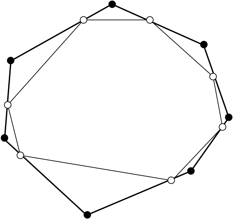
Fig. 1.1: The $E$-construction (thick edges) applied to a polygon (thin edges).

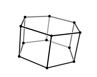
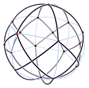
Fig. 1.2: A polytope and its $E$-sphere (in bold, the polytope is drawn thin to show the old ridges).

In dimensions $d\geq 3$ all vertices of the original polytope are preserved, while for $d=2$ they lie on the new edges. A more formal definition given on the level of face lattices is in [PZ04, Def. 1.2]. For any polytope $P$ the sphere $E(P)$ is a piecewise linear CW sphere [PZ04, Thm. 2.1]. If these spheres are polytopal then we call the resulting polytope the $E$-polytope of $P$. This is e.g.  the case for all dual-to-stacked $4$-polytopes [PZ04, Sect. 3]. The $f$-vector of $E(P)$ is given by

$$f_{k}(E(P)):=\begin{cases}f_{d-2}(P)\qquad&k=d-1\\ f_{d-3,d-1}(P)&k=d-2\\ f_{k}(P)+f_{k-1,d-1}(P)\quad&\text{otherwise,}\end{cases}$$

where we set $f_{-1j}:=f_{j}$.

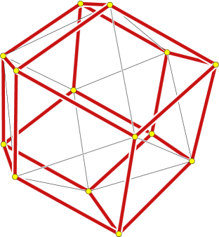
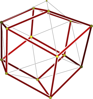
Fig. 1.3: The left realisation of $E(C)$ of the unit cube $C$ is vertex-preserving, the right is not: observe the top vertex of the cube (and there is no cube for which it is).

In the above definition the $E$-polytope of some polytope $P$ just denotes some polytope being combinatorially equivalent to the sphere obtained from $P$ via the $E$-construction. In the following we need a stricter version of the connection between $P$ and its $E$-polytope.

Definition 1.1 (vertex-preserving).

A polytopal realisation of $E(P)$ for a given geometrically realised polytope $P$ is called vertex-preserving if it is obtained from the realisation of $P$ by placing new vertices beyond the facets of $P$ and taking the convex hull. See Figure 1.3 for an example.

Remark 1.2.

For illustrations we will sometimes also apply the $E$-construction to a $1$-polytope $S$ (i.e. a segment). In this case $E(S)$ is defined to be a segment containing $S$ in its interior.

Polygons.

We denote a (convex) polygon with $m$ vertices $v_{0},\ldots,v_{m-1}$ by $C_{m}$. We usually assume that the vertices are numbered consecutively and take indices modulo $m$.

By $E_{mn}$ we denote the result of the $E$-construction applied to the product $C_{m}\times C_{n}$ of an $m$-gon and an $n$-gon. This is a $4$-dimensional $2$-simplicial and $2$-simple $CW$ sphere. The flag vectors of $C_{m}\times C_{n}$ and $E_{mn}$ are:

$$\operatorname{flag}(C_{m}\!\times\!C_{n}) \!=\!(mn,2mn,mn+m+n,m+n;4mn)$$

$$\operatorname{flag}(E_{mn}) \!=\!(mn\!+\!m\!\!+\!n,6mn,6mn,mn\!+\!m\!+\!n;8mn\!+\!2(m\!+\!n)),$$ (1)

where we have only recorded the values $(f_{0},\ldots,f_{3};f_{03})$. All other entries of the flag vector follow from the generalised Dehn-Sommerville equations [BB85].

2 The $E$-construction of products

Let $P_{0}$, $P_{1}$ be two polytopes of dimensions $d_{0}$ and $d_{1}$. We give sufficient conditions for the existence of a polytopal realisation of the sphere $E(P_{0}\times P_{1})$ obtained from the polytope $P_{0}\times P_{1}$. If we restrict to vertex-preserving realisations, then these conditions are also necessary. The conditions are the following:

(A) There exist vertex-preserving realisations of $E(P_{0})$ and $E(P_{1})$. (B) For $i=0,1$ let $T_{i}:=V(E(P_{i}))\setminus V(P_{i})$. There are two maps $\displaystyle\beta_{i}:T_{i}\rightarrow\operatorname{int}(P_{1-i})$ such that for any $(v_{0},v_{1})\in T_{0}\times T_{1}$ the fraction of the segment $|v_{0},\beta_{1}(v_{1})|$ outside $P_{0}$ equals the fraction of the segment $|v_{1},\beta_{0}(v_{0})|$ inside $P_{1}$.

Theorem 2.1.

Let $P_{0}$, $P_{1}$ be a pair of polytopes with $\dim(P_{0}\times P_{1})\geq 3$ that satisfies (A) and (B). Let $S\subset\mathbb{R}^{d_{0}}\times\mathbb{R}^{d_{1}}$ be the point set containing the following points:

1. all pairs $(p_{0},p_{1})$ for $p_{0}\in V(P_{0})$, $p_{1}\in V(P_{1})$,

2. all pairs $(v_{0},\beta_{0}(v_{0}))$ for $v_{0}\in T_{0}$,

3. all pairs $(\beta_{1}(v_{1}),v_{1})$ for $v_{1}\in T_{1}$.

Then $\operatorname{conv}(S)$ is a vertex-preserving polytopal realisation of $E(P_{0}\times P_{1})$. Moreover, for the existence of vertex-preserving realisations of $E(P_{0}\times P_{1})$ the two conditions (A) and (B) are both necessary and sufficient.

See Figure 2.1 for an example of two triangles satisfying (A) and (B).

\psfrag{P1}[l][l]{{$\scriptstyle P_{1}$}}\psfrag{P0}{\hbox{\pagecolor[rgb]{1,1,1}$\scriptstyle P_{0}$}}\psfrag{EP1}{{$\scriptstyle E(P_{1})$}}\psfrag{EP0}{\hbox{\pagecolor[rgb]{1,1,1}$\scriptstyle E(P_{0})$}}\psfrag{v01}[r][r]{\hbox{\pagecolor[rgb]{1,1,1}$\scriptstyle v_{0}^{1}$}}\psfrag{v02}[l][l]{\hbox{\pagecolor[rgb]{1,1,1}$\scriptstyle v_{0}^{2}$}}\psfrag{v03}[rb][rb]{\hbox{\pagecolor[rgb]{1,1,1}$\scriptstyle v_{0}^{3}$}}\psfrag{v11}[r][r]{\hbox{\pagecolor[rgb]{1,1,1}$\scriptstyle v_{1}^{1}$}}\psfrag{v12}[l][l]{\hbox{\pagecolor[rgb]{1,1,1}$\scriptstyle v_{1}^{2}$}}\psfrag{v13}[l][l]{\hbox{\pagecolor[rgb]{1,1,1}$\scriptstyle v_{1}^{3}$}}\psfrag{T1v1}[bl][bl]{\hbox{\pagecolor[rgb]{1,1,1}$\scriptstyle\beta_{1}(v_{1}^{1})$}}\psfrag{T1v2}[bl][bl]{\hbox{\pagecolor[rgb]{1,1,1}$\scriptstyle\beta_{1}(v_{1}^{2})$}}\psfrag{T1v0}[b][b]{\hbox{\pagecolor[rgb]{1,1,1}$\scriptstyle\beta_{1}(v_{1}^{3})$}}\psfrag{T0v1}{\hbox{\pagecolor[rgb]{1,1,1}$\scriptstyle\beta_{0}(v_{0}^{1})$}}\psfrag{T0v2}[rb][rb]{\hbox{\pagecolor[rgb]{1,1,1}$\scriptstyle\beta_{0}(v_{0}^{2})$}}\psfrag{T0v3}[b][b]{\hbox{\pagecolor[rgb]{1,1,1}$\scriptstyle\beta_{0}(v_{0}^{3})$}}\psfrag{q0}{\hbox{\pagecolor[rgb]{1,1,1}$\scriptstyle q_{0}$}}\psfrag{q1}{\hbox{\pagecolor[rgb]{1,1,1}$\scriptstyle q_{1}$}}\includegraphics[height=151.76854pt]{pfp-img-6}

\psfrag{P1}[l][l]{{$\scriptstyle P_{1}$}}\psfrag{P0}{\hbox{\pagecolor[rgb]{1,1,1}$\scriptstyle P_{0}$}}\psfrag{EP1}{{$\scriptstyle E(P_{1})$}}\psfrag{EP0}{\hbox{\pagecolor[rgb]{1,1,1}$\scriptstyle E(P_{0})$}}\psfrag{v01}[r][r]{\hbox{\pagecolor[rgb]{1,1,1}$\scriptstyle v_{0}^{1}$}}\psfrag{v02}[l][l]{\hbox{\pagecolor[rgb]{1,1,1}$\scriptstyle v_{0}^{2}$}}\psfrag{v03}[rb][rb]{\hbox{\pagecolor[rgb]{1,1,1}$\scriptstyle v_{0}^{3}$}}\psfrag{v11}[r][r]{\hbox{\pagecolor[rgb]{1,1,1}$\scriptstyle v_{1}^{1}$}}\psfrag{v12}[l][l]{\hbox{\pagecolor[rgb]{1,1,1}$\scriptstyle v_{1}^{2}$}}\psfrag{v13}[l][l]{\hbox{\pagecolor[rgb]{1,1,1}$\scriptstyle v_{1}^{3}$}}\psfrag{T1v1}[bl][bl]{\hbox{\pagecolor[rgb]{1,1,1}$\scriptstyle\beta_{1}(v_{1}^{1})$}}\psfrag{T1v2}[bl][bl]{\hbox{\pagecolor[rgb]{1,1,1}$\scriptstyle\beta_{1}(v_{1}^{2})$}}\psfrag{T1v0}[b][b]{\hbox{\pagecolor[rgb]{1,1,1}$\scriptstyle\beta_{1}(v_{1}^{3})$}}\psfrag{T0v1}{\hbox{\pagecolor[rgb]{1,1,1}$\scriptstyle\beta_{0}(v_{0}^{1})$}}\psfrag{T0v2}[rb][rb]{\hbox{\pagecolor[rgb]{1,1,1}$\scriptstyle\beta_{0}(v_{0}^{2})$}}\psfrag{T0v3}[b][b]{\hbox{\pagecolor[rgb]{1,1,1}$\scriptstyle\beta_{0}(v_{0}^{3})$}}\psfrag{q0}{\hbox{\pagecolor[rgb]{1,1,1}$\scriptstyle q_{0}$}}\psfrag{q1}{\hbox{\pagecolor[rgb]{1,1,1}$\scriptstyle q_{1}$}}\includegraphics[height=151.76854pt]{pfp-img-7}

Fig. 2.1: Realising the product of two triangles

Proof.

The proof has two parts. First we prove the necessity of the two conditions (A) and (B) for vertex preserving realisations and then their sufficiency.

Let $P_{0}$ and $P_{1}$ be two geometrically realised polytopes of dimension $d_{0}$ and $d_{1}$ with $d_{0}+d_{1}~{}\geq~{}3$. Suppose $E(P_{0}\times P_{1})$ exists and is a vertex-preserving realisation of $P_{0}\times P_{1}$. We can split the vertex set of $E(P_{0}\times P_{1})$ into the vertex set of $P_{0}\times P_{1}$ and a set consisting of one vertex beyond each facet of $P_{0}\times P_{1}$.

Define standard projections $\pi_{j}:\mathbb{R}^{d_{0}+d_{1}}\longrightarrow\mathbb{R}^{d_{j}}$ for $j=0,1$. By assumption, the vertex set of $P_{j}$ is contained in $\pi_{j}(V(E(P_{0}\times P_{1})))$ for $j=0,1$. We determine the images of the other vertices of $E(P_{0}\times P_{1})$ under $\pi_{0}$ and $\pi_{1}$.

The facets of the product $P_{0}\times P_{1}$ are of the form (1) “Facet of $P_{0}$” $\times P_{1}$ or (2) $P_{0}\times$“Facet of $P_{1}$”. Thus, we have two different types of ridges: (I) Those between two adjacent facets of the first or second type, and (II) those between a facet of the first and one of the second type. We deal with these two cases separately:

1. Let $F$ and $F^{\prime}$ be two adjacent facets of the first type and $v$, $v^{\prime}$ the two vertices of $E(P_{0}\times P_{1})$ beyond $F$ and $F^{\prime}$. Let $R$ be the ridge between $F$ and $F^{\prime}$. The projections $\pi_{0}(F)$ and $\pi_{0}(F^{\prime})$ are adjacent facets of $P_{0}$ with common ridge $\pi_{0}(R)$. $\pi_{0}(v)$ and $\pi_{0}(v^{\prime})$ are points beyond these facets. $v$, $v^{\prime}$ and $R$ lie on a common (facet defining) hyperplane $H$ of $E(P_{0}\times P_{1})$ in $\mathbb{R}^{d_{0}+d_{1}}$. So the points $\pi_{0}(v)$, $\pi_{0}(v^{\prime})$ and the ridge $\pi_{0}(R)$ all lie on the hyperplane $\pi_{0}(H)$ in $\mathbb{R}^{d_{0}}$ and $\pi_{0}(H)$ defines a face of $\pi_{0}(E(P_{0}\times P_{1}))$, which must in fact be a facet. Thus, the convex hull of the projection of all vertices of $E(P_{0}\times P_{1})$ is $E(P_{0})$. Similarly, projecting with $\pi_{1}$ gives $E(P_{1})$.

2. Let $w_{0}$ and $w_{1}$ be two vertices of $E(P_{0}\times P_{1})$, the first beyond a facet $G_{0}\times P_{1}$, the second beyond $P_{0}\times G_{1}$, where $G_{0}$ and $G_{1}$ are facets of $P_{0}$ and $P_{1}$. Let $R=G_{0}\times G_{1}$ be the ridge between these two facets. The segment $s$ between $w_{0}$ and $w_{1}$ intersects $R$ in a point $q$. $\pi_{0}(q)$ is contained in $G_{0}$ and $\pi_{1}(q)$ is contained in $G_{1}$. So $\pi_{0}(w_{1})$ is contained in the interior of $P_{0}$ and $\pi_{1}(w_{0})$ in the interior of $P_{1}$. Projections preserve ratios, so

   $$r:=\frac{|w_{0}q|}{|w_{0}w_{1}|}=\frac{|\pi_{0}(w_{0})\pi_{0}(q)|}{|\pi_{0}(w_{0})\pi_{0}(w_{1})|}=\frac{|\pi_{1}(w_{0})\pi_{1}(q)|}{|\pi_{1}(w_{0})\pi_{1}(w_{1})|}.$$

Hence, a vertex-preserving realisation of $E(P_{0}\times P_{1})$ implies the conditions (A) and (B). This proves the necessity part of the theorem.

Now we prove sufficiency of (A) and (B). Suppose we have, according to (A) and (B), constructed $E(P_{0})$ and $E(P_{1})$ and the maps $\beta_{i}:T_{i}\rightarrow\operatorname{int}(P_{1-i})$ for $T_{i}:=V(E(P_{i}))\setminus V(P_{i})$, $i=0,1$, and have formed the set $S$ defined in the theorem. We have to show that all facets of the convex hull of $S$ defined thereby are bipyramids over ridges of $P_{0}\times P_{1}$ and that there is precisely one vertex of $S$ beyond each facet of $P_{0}\times P_{1}$. There are two different cases to consider:

1. Let $R$ be a ridge of $P_{0}$. Then $R\times P_{1}$ is a ridge of $P_{0}\times P_{1}$. Let $F$ and $F^{\prime}$ be the two facets of $P_{0}$ adjacent to $R$ and $p$, $p^{\prime}$ the vertices of $E(P_{0})$ above $F$ and $F^{\prime}$ (see Figure 2.2). Let $v$ be the facet normal of the facet $F_{E}$ of $E(P_{0})$ formed by $R$, $p$ and $p^{\prime}$ and let $l:=\langle v,p\rangle$.

   \psfrag{R}{$R$}\psfrag{F0}{$F$}\psfrag{F1}{$F^{\prime}$}\psfrag{p0}{$p$}\psfrag{p1}{$p^{\prime}$}\psfrag{v}{$v$}\includegraphics[width=108.405pt]{pfp-img-8}

   Fig. 2.2: Sufficiency: The case of “ridge $\times$ polytope”

   By construction, the points $(p,\beta_{0}(p))$, $(p^{\prime},\beta_{0}(p^{\prime}))$ and $(r,q)$, $r\in V(R)$, $q\in V(P_{1})$ are contained in the hyperplane $H:=\{x\mid\langle(v,\mathbf{0}),x\rangle=l\}$, where $\mathbf{0}$ denotes the $d_{1}$-dimensional zero vector. All points in the set $V(E(P_{0}))\setminus(V(R)\cup\{p,p^{\prime}\})$ are on the same side of the hyperplane defined by the facet $F_{E}$. So all points in

   $$V(E(P_{0}\times P_{1}))\setminus(V(R\times P_{1})\cup\{(p,\beta_{0}(p)),(p^{\prime},\beta_{0}(p^{\prime}))\})$$

   are on the same side of the hyperplane $H$ and

   $$\operatorname{conv}(V(R\times P_{1})\cup\{(p,\beta_{0}(p)),(p^{\prime},\beta_{0}(p^{\prime}))\})$$

   is a facet of $E(P_{0}\times P_{1})$. The same argument applies to ridges of type $P_{0}\times R$ for ridges $R$ of $P_{1}$.

2. Now consider a ridge of type $F_{0}\times F_{1}$ for a facet $F_{0}$ of $P_{0}$ and a facet $F_{1}$ of $P_{1}$. Let $p_{0}$ be the vertex of $E(P_{0})$ beyond $F_{0}$ and $p_{1}$ the vertex of $E(P_{1})$ beyond $F_{1}$. Let $i_{0}$ be the intersection point of the segment between $p_{0}$ and $\beta_{1}(p_{1})$ and the facet $F_{0}$, and $i_{1}$ the intersection point of the segment between $p_{1}$ and $\beta(p_{0})$ and the facet $F_{1}$. By construction we have

   $$\frac{|p_{0},i_{0}|}{|p_{0},\beta_{1}(p_{1})|}=\frac{|\beta_{0}(p_{0}),i_{1}|}{|\beta_{0}(p_{0}),p_{1}|}$$

   and the point $(p_{0},\beta_{0}(p_{0}))$ is contained in the line defined by $(\beta_{1}(p_{1}),p_{1})$ and $(i_{0},i_{1})$. So the points $V(F_{0}\times F_{1})$, $(p_{0},\beta_{0}(p_{0}))$ and $(\beta_{1}(p_{1}),p_{1})$ lie on a common hyperplane $H$.

   The product $P_{0}\times P_{1}$ lies entirely on one side of $H$ by construction. Suppose there is a point $x$ of $S$ on the other side of $H$. As $H$ is a valid hyperplane for the ridge $F_{0}\times F_{1}$, any point beyond it is also beyond either the facet hyperplane of $F_{0}\times P_{1}$ or $P_{0}\times F_{1}$. Assume the first. For any $z\in S$ we have either $\pi_{0}(z)\in S_{1}$, or $\pi_{0}(z)\in V(P_{0})$, or $\pi_{0}(z)\in V(E(P_{0}))\setminus V(P_{0})$. $x\in S$ is beyond $F_{0}\times P_{1}$, therefore only $\pi_{0}(x)\in V(E(P_{0}))\setminus V(P_{0})$ is possible. Thus, $\pi_{0}(x)$ is the unique vertex of $E(P_{0})$ beyond $F_{0}$, so $\pi_{0}(x)=p_{0}$ and $x\in H$.

This proves that the two conditions (A) and (B) are sufficient for the existence of a polytopal realisation of $E(P_{0}\times P_{1})$.∎

In Section 4.4 we present some general applications of Theorem 2.1. However, we mostly use a more restrictive version of it. We tighten the conditions (A) and (B) in the following way to make them more manageable:

(A^′) There exist vertex-preserving realisations of $E(P_{0})$ and $E(P_{1})$. (B^′) For $i=0,1$ let $T_{i}:=V(E(P_{i}))\setminus V(P_{i})$. There are points $s_{i}\in\operatorname{int}(P_{i})$ and some $0<r<1$ such that for any $v_{0}\in T_{0}$ and $v_{1}\in T_{1}$ $\displaystyle r|s_{0},v_{0}|=|s_{0},q_{0}|\qquad\qquad(1-r)|s_{1},v_{1}|=|s_{1},q_{1}|,$ where $q_{i}$ is the intersection of the segment from $s_{i}$ to $v_{i}$ and $|a,b|$ denotes the length of the segment from $a$ to $b$ (Hence $\beta_{i}(x)\equiv s_{i}$ for $i=0,1$).

Theorem 2.1 immediately implies the following.

Corollary 2.2.

Let $P_{0}$, $P_{1}$ be a pair of polytopes with $\dim(P_{0}\times P_{1})\geq 3$ that satisfies (A) and (B). Let $S\subset\mathbb{R}^{d_{0}}\times\mathbb{R}^{d_{1}}$ be the point set containing the following points:

1. all pairs $(p_{0},p_{1})$ for $p_{0}\in V(P_{0})$, $p_{1}\in V(P_{1})$,

2. all pairs $(v_{0},s_{1})$ for $v_{0}\in T_{0}$,

3. all pairs $(s_{0},v_{1})$ for $v_{1}\in T_{1}$.

Then $\operatorname{conv}(S)$ is a vertex-preserving polytopal realisation of $E(P_{0}\times P_{1})$.∎

In this setting, the only connection between the construction of the two factors is the value $r$ of the ratio. Thus, if we construct a polytope $P$ together with a vertex-preserving realisation of $E(P)$ and a single point $s$ in its interior such that all segments from $s$ to the vertices of $E(P)$ not in $P$ intersect $\partial P$ with ratio $r$, then we can combine this with any other such instance for a ratio of $1-r$.

3 Explicit realisations

Now we apply the construction of the previous section and produce examples of products of polytopes with a realisation of their $E$-polytope. The main focus is on the realisation of the $E$-polytope $E_{mn}$ of a product of an $m$-gon and an $n$-gon. We produce polytopal realisations for all of them. Afterwards we briefly discuss examples in dimensions $d\geq 5$. For some of the examples explicit data in the polymake format (Gawrilow and Joswig [GJ00]) are available on request.

3.1 Products of polygons

We begin with products of polygons and present a method to obtain a “flexible” geometric realisation of $E_{mn}:=E(C_{m}\times C_{n})$ for all $m,n\geq 3$. We will discuss degrees of freedom in this construction in Section 4.4.

Theorem 3.1.

The CW spheres $E_{mn}$ are polytopal for all $m,n\geq 3$.

In the five cases when $m,n$ satisfy $\frac{1}{m}+\frac{1}{n}\geq\frac{1}{2}$, polytopality follows from a construction of Santos [San03], [San00, Rem. 13]. These realisations are presented in Theorem 4.3.

We use the restricted setting of Corollary 2.2 for the proof and construct only one of the two factors, but subject to the conditions (A^′) and (B^′). We make the following definition for this.

Definition 3.2.

Let $\frac{1}{3}<r<\frac{2}{3}$. By $D(k,r)$ we denote a realisation of a $k$-gon $C_{k}$ together with

• a distinguished inner point $s$,

• a vertex-preserving $E$-polytope $E(C_{k})$, such that segments from $s$ to vertices of $E(C_{k})$ are intersected by the boundary of $C_{k}$ with ratio $r$.

See Figure 3.2 for an example. To realise $E_{mn}$ we choose a ratio $r$ between $\frac{1}{3}$ and $\frac{2}{3}$ and combine the points of $D(m,r)$ and $D(n,1-r)$ according to Corollary 2.2. We restrict to $m\geq 4$ in the following and refer to the proof of Theorem 4.3 for the case $m=3$.

The next construction is illustrated in Figure 3.2. Let $\Gamma$ denote the graph of the parabola $x\mapsto x^{2}$ in the plane $\mathbb{R}^{2}$ with coordinates $x$ and $y$. We construct the polygon $C_{m}$ such that all but one of the vertices lie on $\Gamma$, and $E(C_{m})$ such that all but one of the edges are tangent to $\Gamma$.

Let $s$ be the point $(0,1)$ and define the three functions

$$\mathcal{C}(x) :=\frac{x+\sqrt{(1-r)(2r+rx^{2}+x^{2})}}{r}$$

$$\overline{\mathcal{C}}(x) :=\frac{x(x+\sqrt{x^{2}+2r^{2}x^{2}-2rx^{2}-2r+2r^{2}}-rx)}{r}$$

$$\mathcal{E}(x) :=\frac{x+\sqrt{x^{2}+2r^{2}x^{2}-2rx^{2}-2r+2r^{2}}}{2r}.$$

For any $a\geq 0$ let $p(a)\in\mathbb{R}^{2}$ be the intersection point of the tangents to $\Gamma$ in $(a,a^{2})$ and $(\mathcal{C}(a),\mathcal{C}(a)^{2})$. We have the following facts about these functions.

Lemma 3.3.

Let $0<r<\frac{2}{3}$.

1. For any $a\geq 0$ the secant line between $(a,a^{2})$ and $(\mathcal{C}(a),\mathcal{C}(a)^{2})$ intersects the segment between $s$ and $p(a)$ in a point $q(a)$ satisfying

   $$r|s,p(a)|=|s,q(a)|,$$

   where $|x_{0},x_{1}|$ denotes the length of the segment between $x_{0}$ and $x_{1}$.

2. For any $a\geq 1$ the line between $(a,a^{2})$ and $(0,\overline{\mathcal{C}}(a))$ intersects the segment between $s$ and $\overline{p}(a):=(\overline{\mathcal{C}}(a),\mathcal{E}(a))$ in a point $\overline{q}(a)$ satisfying

   $$r|s,\overline{p}(a)|=|s,\overline{q}(a)|.$$

3. For any $a\geq 0$ we have $\mathcal{C}(a)>1$.

4. For any $a>1$ we have $\overline{\mathcal{C}}(a)>a^{2}$.

5. For any $a>1$ we have $\overline{\mathcal{C}}(x)=2x\mathcal{E}(x)-x^{2}$. ∎

\psfrag{E}{$E(\Delta)$}\psfrag{D}{$\Delta$}\psfrag{S}{$s$}\includegraphics[width=429.28616pt]{pfp-img-9}

Fig. 3.1: An example of a realisation of $D(3,\frac{1}{3})$.

\psfrag{s}[b][b]{$s$}\psfrag{v0}[t][t]{$v_{0}$}\psfrag{v1m}[tr][tr]{$v_{1}^{-}$}\psfrag{v1p}[tl][tl]{$v_{1}^{+}$}\psfrag{v2m}[tr][tr]{$v_{2}^{-}$}\psfrag{v2p}[tl][tl]{$v_{2}^{+}$}\psfrag{v3}[b][b]{$v_{3}$}\psfrag{C}[br][br]{$C_{6}$}\psfrag{E}[b][b]{$E(C_{6})$}\psfrag{pbv}[l][l]{$\overline{p}((v_{2}^{+})_{x})$}\psfrag{qbv}[r][r]{$\overline{q}((v_{2}^{+})_{x})$}\psfrag{pv}[l][l]{$p((v_{1}^{+})_{x})$}\includegraphics[width=411.93767pt]{pfp-img-10}

Fig. 3.2: The construction of $D(6,\frac{3}{5})$. Note that the $x$-axis has larger scale than the $y$-axis.

With this information at hand we are ready to give an iterative construction for $D(m,r)$ in the case $m\geq 4$ and $0<r<\frac{2}{3}$. We distinguish the two cases $m$ even and $m$ odd.

• For $m$ even we choose the point $v_{0}^{+}:=(0,0)$ as our first vertex of $C_{m}$, for $m$ odd we take the two points $v_{0}^{\pm}:=(\pm\sqrt{\frac{1-r}{1+r}},\frac{1-r}{1+r})$.

• In the $i$-th step we extend with the points $v_{i}^{\pm}:=(\pm\mathcal{C}(a),\mathcal{C}(a)^{2})$, where $a$ is the $x$-coordinate of $v_{i-1}^{+}$.

• We repeat the previous step until we have constructed $m-1$ points of $C_{m}$.

• In the last step we add the vertex $v_{\lfloor\frac{m}{2}\rfloor}:=(0,\overline{\mathcal{C}}(a))$, where $a$ is the $x$-coordinate of $v_{\lfloor\frac{m}{2}\rfloor-1}$.

The edges of $E(C_{m})$ are the tangents to $\Gamma$ in the vertices of $C_{m}$, except for $v_{\lfloor\frac{m}{2}\rfloor}$, where we take the horizontal line running through $v_{\lfloor\frac{m}{2}\rfloor}$. This line intersects the tangents to $(v_{m-1}^{\pm},(v_{m-1}^{\pm})^{2})$ in the points $(\pm\mathcal{E}(v_{m-1}^{+}),\overline{\mathcal{C}}(v_{m-1}^{+}))$.

Lemma 3.3 guarantees the condition on the intersection ratio. The point $s=(0,1)$ is inside $C_{m}$ by Lemma 3.3(3),(5). Hence we can construct $D(m,r)$ for $0<r<\frac{2}{3}$ and $m\geq 4$. Finally, a realisation for $m=3$ and $\frac{1}{4}<r<1$ is given in the proof of Theorem 4.3. By combining $D(n,r)$ with $D(m,1-r)$ for some $m\geq 3$ we obtain $E_{mn}$. This proves Theorem 3.1.

Remark 3.4.

$D(m,r)$ can in fact be constructed for any $r$ between $0$ and $1$ and any $m\geq 3$, but the formulas for the vertices and the cases one has to distinguish in the construction tend to get complicated rather quickly.

3.2 Some higher-dimensional examples

Satisfying the conditions (A) and (B) is more difficult if the two factors $P_{0}$ and $P_{1}$ have more facets. Thus in higher dimensions and for “more complex” polytopes, it is usually hard to find maps $\beta_{0}$ resp.  $\beta_{1}$, unless one can exploit some kind of symmetry.

There are, however, two obvious families of polytopes that we can choose as factors of a product polytope: The $d$-simplex $\Delta_{d}$ and the $d$-cube $C_{d}$. Both can be realised together with their $E$-construction satisfying even the restrictive conditions of Corollary 2.2.

• The cube with its $E$-construction and an intersection ratio of $r=\frac{1}{2}$ can be realised as follows: For $C_{d}$ we take the standard $\pm 1$-cube. The new vertices for the $E$-polytope are $\pm 2\cdot e_{i}$, where $e_{i}$ are the standard unit basis vectors. The origin is an inner point $s$ satisfying all requirements.

• The construction for the $d$-simplex $\Delta_{d}$ is slightly more difficult. We give an inductive construction that produces realisations for any ratio $\frac{1}{2}\leq r<1$, that is, at least half of the segment is inside $\Delta$ (where $r$ is the parameter appearing in the conditions in the box on page 2). We can clearly construct such a realisation for a triangle, i.e. for a simplex of dimension $d=2$.

  For $d>2$ we take a regular realisation $\Delta$ of the simplex and a scaled version $\Delta^{\prime}:=\frac{1}{r}\cdot\Delta$ with the same barycentre. We choose one facet $F$ of $\Delta$ and the corresponding scaled facet $F^{\prime}$ in $\Delta^{\prime}$. Place the first new vertex $v$ in the barycentre of $F^{\prime}$. The vertices of any ridge $R$ of $F$ together with the point $v$ uniquely define a hyperplane. $F$ has $d$ ridges, so we obtain $d$ different hyperplanes $H_{1},\ldots,H_{d}$ by this. $H_{1},\ldots,H_{d}$ intersect all facet hyperplanes of $\Delta^{\prime}$, except that to $F^{\prime}$, in codimension-2-planes that lie in a common hyperplane $H$. $H$ is parallel to $F$.

  $H$ cuts $\Delta$ and $\Delta^{\prime}$ in two simplices $\tilde{\Delta}$ and $\tilde{\Delta}^{\prime}$ of dimension $d-1$. (Recall that $r\geq\frac{1}{2}$, so $H$ intersects $\Delta$ below the barycentre if viewed from $F$.) $\tilde{\Delta}^{\prime}$ is (viewed in the hyperplane $H$) a scaled version of $\tilde{\Delta}$ with a scaling factor $\frac{1}{r^{\prime}}\leq\frac{1}{r}$. By induction, we have a solution for the corresponding problem for $\tilde{\Delta}$ and $r^{\prime}\geq r\geq\frac{1}{2}$ in $H$ (where the inner point is the projection of the barycentre of $\Delta$).

  These points, together with the one vertex $v$ chosen before, give a realisation of $E(\Delta)$ that satisfies the conditions of Corollary 2.2. See Figure 3.3 for the case $d=3$.

\psfrag{v}{$v$}\psfrag{H}[t][t]{$H$}\psfrag{Dp}[r][r]{$\Delta^{\prime}$}\psfrag{D}[r][r]{$\Delta$}\psfrag{F}[r][r]{$F$}\psfrag{Fp}[tl][tl]{$F^{\prime}$}\includegraphics[height=166.94463pt]{pfp-img-11}

Fig. 3.3: The construction for a $3$-simplex. The solution for $d=2$ used in the plane $H$ is indicated with thin lines.

We can combine such a simplex or cube with another simplex, cube or some $D(n,\frac{1}{2})$ to obtain the $E$-polytope of this product.

4 Properties of the family $E_{mn}$

This section collects several properties of the polytopes $E_{mn}$. In particular we count degrees of freedom for the realisation of $E_{33}$ and prove that not all combinatorial symmetries of $E_{mn}$ are geometrically realisable.

4.1 Self-duality

The polytopes $C_{m}\times C_{n}$ are simple, thus we know from [PZ04, Thm. 1.6] that $E_{mn}$ is $2$-simple and $2$-simplicial (that is, all $2$-faces are triangles and all edges are in $3$ facets). In particular the $f$-vector of $E_{mn}$ is symmetric (cf. Eq. (1)).

The polytopes $E_{mn}$ are in fact self-dual. This is not true for arbitrary $2$-simple, $2$-simplicial polytopes, which can be seen from the hypersimplex $E(\Delta)$ obtained from the $4$-simplex $\Delta$. This polytope has a facet-transitive automorphism group acting on its 10 bipyramidal facets, while the dual has 5 tetrahedral and 5 octahedral facets.

Theorem 4.1 (Ziegler [Zie03]).

Each of the polytopes $E_{mn}$ ($n,m\geq 3$) is self-dual, with an anti-automorphism of order $2$.

Proof.

Number the vertices of an $k$-gon $C_{k}$ consecutively by $v_{0},\ldots,v_{k-1}$. We take indices modulo $k$. The vertices of $C_{m}\times C_{n}$ are $v_{i,j}:=(v_{i},v_{j})$ for $0\leq i\leq m-1$ and $0\leq j\leq n-1$. We have two types of facets in the product:

$$F^{\prime}_{i} =\operatorname{conv}(\{v_{ij},v_{i+1,j}\mid j=0,\ldots,n-1\})$$

$$F^{\prime\prime}_{j} =\operatorname{conv}(\{v_{ij},v_{i,j+1}\mid i=0,\ldots,m-1\}).$$

We denote the new vertex beyond $$F^{\prime}_{i} v^{\prime}_{i} F^{\prime\prime}_{i} v^{\prime\prime}_{i} E(C_{m}\times C_{n})$$ by and the one beyond by . The facets of are now of the form

$$G_{ij} =\operatorname{conv}(v_{ij},v_{i+1,j},v_{i,j+1},v_{i+1,j+1},v^{\prime}_{i},v^{\prime\prime}_{j})$$

$$G^{\prime}_{i} =\operatorname{conv}(\{v_{ij}\mid j=0,\ldots,n-1\},v^{\prime}_{i-1},v^{\prime}_{i})$$

$$G^{\prime\prime}_{j} =\operatorname{conv}(\{v_{ij}\mid i=0,\ldots,m-1\},v^{\prime\prime}_{j-1},v^{\prime\prime}_{j}).$$

From this we can read off the facets a vertex is contained in:

$$v_{ij} \in G_{ij},G_{i-1,j},G_{i,j-1},G_{i-1,j-1},G^{\prime}_{i-1},G^{\prime\prime}_{j-1}$$

$$v^{\prime}_{i} \in G^{\prime}_{i},G^{\prime}_{i+1},G_{ij}\text{ for }j=0,\ldots,n-1$$

$$v^{\prime\prime}_{j} \in G^{\prime\prime}_{j},G^{\prime\prime}_{j+1},G_{ij}\text{ for }i=0,\ldots,m-1.$$

Thus the following correspondence gives a self-duality of order $2$:

$$G_{ij} \longleftrightarrow v_{-i,-j}\qquad G^{\prime}_{i}\longleftrightarrow v^{\prime}_{-i}\qquad G^{\prime\prime}_{j}\longleftrightarrow v^{\prime\prime}_{-j}\qed$$

For $m=n$, this result was obtained previously by Gévay [Gev04].

Remark 4.2.

There are examples of $3$-polytopes that are self-dual, but that do not have a self-duality of order $2$ (cf. [Grü03, Ex. 3.4.3, p.52d]).

4.2 $E_{mn}$ constructed from regular polygons

Only in a few cases there are “more symmetric” realisations of the polytopes $E_{mn}$: We prove that there are only five choices of pairs $(m,n)$ (up to interchanging $m$ and $n$) such that we can take regular polygons as input for the construction described in Theorem 2.1 in the restricted version of Corollary 2.2. We will see in the next section that these five cases are also the only cases in which the product of two cyclic groups induced from rotation of the vertices in the two factors can be a subgroup of the geometric symmetry group. The next theorem is based on Santos [San00, Rem. 13], [San03].

Theorem 4.3.

There are polytopal realisations of $E_{mn}$ for which projection onto the first and last two coordinates yields in both cases

1. regular polygons for the polygon in $C_{m}\times C_{n}$ and its $E$-construction,

2. and all intersection ratios are equal in each factor

if and only if $\frac{1}{m}+\frac{1}{n}\geq\frac{1}{2}$.

\psfrag{s}{$l$}\psfrag{P}{$P$}\psfrag{EP}{$E(P)$}\includegraphics[width=93.89418pt]{pfp-img-12}

\psfrag{s}{$l$}\psfrag{P}{$P$}\psfrag{EP}{$E(P)$}\includegraphics[width=85.35826pt]{pfp-img-13}

Fig. 4.1: Two projections that satisfy the restrictions of Theorem 4.3

Proof.

The condition on the ratio implies that the images of the maps $\beta_{0}$ and $\beta_{1}$ appearing in the construction of $E_{mn}$ are single points in the interior of the polygons $C_{m}$ and $C_{n}$. These points must be the barycentres if the polygons are regular. We may assume that this is the origin.

We can now generate all configurations of a regular polygon $C_{m}$ together with $E(C_{m})$ in the following way: Start with a regular polygon $E(C_{m})$ centred at the origin and choose a vertex for $C_{m}$ on each of the edges. As $C_{m}$ is regular, the vertices of $C_{m}$ divide each edge with equal ratio. The segments considered in (B) are the segments $l$ between the origin and a vertex of $E(C_{m})$. We are interested in the possible values of the ratio with which they are intersected by the edges of $C_{m}$.

Choosing the vertices of $C_{m}$ close to those of $E(C_{m})$ we see that we can have an arbitrarily high portion of $l$ inside $C_{m}$. On the other hand, the portion inside $C_{m}$ is minimised when we place the vertices of $C_{m}$ in the centre of the edges. In this case, the fraction of $l$ outside $C_{m}$ is $\sin^{2}(\frac{\pi}{n})$. By condition (B), the fraction lying outside for one polygon and its $E$-construction has to match the fraction lying inside for the other polygon. This gives the following inequalities:

$$1-\sin^{2}\left(\frac{\pi}{m}\right)\leq\sin^{2}\left(\frac{\pi}{n}\right)\qquad\text{and}\qquad 1-\sin^{2}\left(\frac{\pi}{n}\right)\leq\sin^{2}\left(\frac{\pi}{m}\right),$$

which are equivalent to the condition given in the theorem. ∎

We can determine all possible values for the inequalities of the theorem explicitly.

Corollary 4.4.

There are realisations of $E_{mn}$ from regular polytopes only for the following pairs $(m,n)$ (up to interchanging $m$ and $n$):

$$(3,3)\;,\;(3,4)\;,\;(3,5)\;,\;(3,6)\;,\;(4,4)$$ ∎

Remark 4.5.

We made assumption (2) in Theorem 4.3 mainly because this is the case we need in the next section. A less restrictive version of “symmetry” would only require the points in the images of $\beta_{0}$ and $\beta_{1}$ to also form regular polygons (if we take the points in the order induced by the $E$-construction of the other factor). For small $m=n$ this has solutions where all points in the images are different. See Table 4.3 for an example of an $E_{44}$. Note however, that this severely reduces the number of geometric symmetries compared to the case of the theorem.

4.3 Combinatorial versus geometric symmetries

There are two different notions of symmetry for a polytope $P$.

Definition 4.6.

Let $P$ be a polytope with a given geometric realisation. Any affine transformation $T$ of the ambient space that preserves $P$ set-wise is called a geometric symmetry transformation. The group of all such transformations is called the geometric symmetry group.

To any polytope $P$ we can associate the poset of all faces of $P$ ordered by inclusion. This is called the face lattice $F(P)$ of $P$. A combinatorial symmetry of $P$ is an automorphism of $F(P)$. The group of all combinatorial symmetries is the combinatorial symmetry group.

The combinatorial symmetry group is independent of a realisation, while the geometric symmetry group highly depends on the choice of the realisation.

A geometric symmetry maps $k$-faces to $k$-faces and preserves incidences. Therefore any geometric symmetry induces a combinatorial symmetry. On the other hand, a combinatorial symmetry in general does not induce a geometric one. However, there are not many examples known of polytopes where these two groups differ for all possible geometric realisations of a polytope. Bokowski, Ewald, and Kleinschmidt have provided a $4$-dimensional example on $10$ vertices in [BEK84]. Dimension $4$ is smallest possible for such examples, as it is known, that for $3$-polytopes, and for polytopes with few vertices in any dimension, there are realisations for which geometric and combinatorial symmetry group coincide (see [Man71] for the first and [Grü03, p.120] for the second result). We show that our product construction provides an infinite series of $4$-polytopes with non-realisable geometric symmetries. We construct an explicit example of such a symmetry for the proof. Previously it was observed by Gévay that there is no polytopal realisation of the CW spheres $E_{mm}$ with the full symmetry group, except in the case $m=4$. This is also a consequence of Corollary 4.8 below.

Theorem 4.7.

For relatively prime $m,n\geq 5$ all $E_{mn}$ admit combinatorial symmetries that cannot be realised as affine symmetry transformations of a geometric realisation of $E_{mn}$.

The three symmetries involved in the proof of Theorem 4.7 Notation: $\triangleright$ $v_{0},v_{1},v_{2}$: vertices of $C_{3}$ $\triangleright$ $w_{0},w_{1},w_{2},w_{3}$ vertices of $C_{4}$ $\triangleright$ $e(j)$: edge from vertex number $j$ to $j+1$ (mod $3$ or $4$) in both polygons. Number the vertices $p_{k}$ of $P_{34}$ in the following way: $0\leq k\leq 11$: vertices $(v_{k\text{ div }4},w_{k-4(k\text{ div }4)})$ $12\leq k\leq 14$: vertices added above $e(k-12)\times C_{4}$ $15\leq k\leq 19$: vertices added above $C_{3}\times e(k-15)$ Then the combinatorial symmetries are given as (permutation notation, vertex numbers of $p_{k}$): $\displaystyle\tilde{S}_{3}$ $\displaystyle:=(0,4,8)(1,5,9)(2,6,10)(3,7,11)(12,13,14)(15)(16)(17)(18)$ $\displaystyle\tilde{S}_{4}$ $\displaystyle:=(0,1,2,3)(4,5,6,7)(8,9,10,11)(12)(13)(14)(15,16,17,18)$ $\displaystyle T$ $\displaystyle:=(0,5,10,3,4,9,2,7,8,1,6,11)(12,13,14)(15,16,17,18)$

Table 4.1: The combinatorial symmetries $\tilde{S}_{3}$, $\tilde{S}_{4}$, and $T$ acting on $P_{34}$.

Proof.

Let $P_{mn}$ be any geometric realisation of a polytope combinatorially equivalent to an $E_{mn}$. Seen as a PL sphere, $P_{mn}$ can still be viewed as the result of the $E$-construction applied to a PL sphere which is combinatorially equivalent to a product of two polygons.

Here is a non-realisable combinatorial symmetry $T$ of $P_{mn}$. Let $C_{m}$ and $C_{n}$ denote polygons with vertices $v_{0},\ldots,v_{m-1}$ resp.  $w_{0},\ldots,w_{n-1}$ numbered in cyclic order. We take indices modulo $m$ resp. $n$. Let $S$ be the combinatorial symmetry of a polygon that maps the $j$-th to the $(j+1)$-th vertex.

$S$ induces a combinatorial symmetry $S_{m}$ on $C_{m}\times C_{n}$ by mapping a vertex $(v_{i},w_{j})$ to $(v_{i+1},w_{j})$ for any $0\leq j\leq m-1$. Similarly $S$ induces a symmetry $S_{n}$ shifting the vertices of $C_{n}$. Both symmetries uniquely extend to combinatorial symmetries $\tilde{S}_{m}$ and $\tilde{S}_{n}$ of $E(C_{m}\times C_{n})$. Let $T$ be the combinatorial symmetry of $P_{mn}$ obtained by first applying $\tilde{S}_{m}$ and then $\tilde{S}_{n}$. See Table 4.1 for an example.

A geometric realisation of $P_{mn}$ need not have the product structure induced by the construction of Theorem 2.1. However, by looking at vertex degrees, for $m,n\geq 5$ we can decide which of the vertices of $P_{mn}$ “belong” to the product and which are “added” by the $E$-construction: A vertex of the product always has degree $8$, as $C_{m}\times C_{n}$ is simple, so any vertex has four neighbours and is in four facets. The added vertices all have degree $2m$ or $2n$. Denote the vertex sets by $V_{p}$ and $V_{e}$.

The proof is roughly as follows. Suppose there is a geometric realisation $T_{g}$ of $T$ for some $P_{mn}$. First we prove that any $P_{mn}$ having $T_{g}$ as a geometric symmetry has the form of the construction in Theorem 2.1. Then the symmetry implies that both factors are of the form defined in Theorem 4.3. Corollary 4.4 finally tells us that for $m,n\geq 5$ there are no such realisations.

As $T_{g}$ set-wise fixes the the vertices of $P_{mn}$ it also fixes the centroid of the vertices of $P_{mn}$. After a suitable translation we can assume that $T_{g}$ is a linear transformation. As $m$ and $n$ are relatively prime, there is a $k_{m}\in\mathbb{N}$ such that $T_{m}:=T_{g}^{k_{m}}$ restricted to the set $V_{p}$ acts as $\tilde{S}_{m}$. Similarly there is a $k_{n}$ such that $T_{n}:=T_{g}^{k_{n}}$ reduces to a realisation of $\tilde{S}_{n}$. $T_{m}$ and $T_{n}$ are linear transformations.

By construction $P_{mn}$ has two different combinatorial types of facets: Bipyramids over an $m$-gon and over an $n$-gon. For any facet we call the vertices of the polygon (i.e. those vertices of the facet belonging to $V_{p}$) the base vertices.

Let $F$ be a facet of $P_{mn}$ of the first type. The symmetry $T_{m}$ shifts the base vertices by one and fixes the two apices. Thus, $T_{m}$ also fixes the centroid $c_{F}$ of the base vertices of $F$ and $T_{m}$ restricted to the hyperplane $H_{F}$ defined by $F$ is a linear transformation $T_{m}^{F}$ in $H_{F}$ (if we put the origin of $H_{F}$ in $c_{F}$). Now $T_{m}$ fixes the two apices of $F$ and thus fixes the whole line through the apices. So $T_{m}^{F}$ splits into a map fixing the axis and a linear transformation of a two dimensional transversal subspace. The axis must contain $c_{F}$ and the subspace the base vertices of $F$. So the base vertices of $F$ lie in a common two dimensional affine subspace of $\mathbb{R}^{4}$. Similarly, the base vertices of any other bipyramidal facet with a base equivalent to $C_{m}$ lie in a common $2$-plane. These $2$-planes are set-wise preserved by $T_{m}$ and therefore must be parallel.

The same argument proves that all bases of facets combinatorially being bipyramids over $n$-gons do lie in parallel $2$-planes. These $2$-planes must be transversal to the $2$-planes containing the $m$-gons: Otherwise the vertices in $V_{p}$ all lie in a three dimensional subspace. As $P_{mn}$ is four dimensional, at least one of the vertices of $V_{e}$ has to lie outside this $3$-space. But there are no edges between vertices in $V_{e}$.

Applying an appropriate linear transformation to $P_{mn}$ we can assume that the $2$-spaces containing the $m$-gons are parallel to the $x_{1}$-$x_{2}$-plane and the ones containing the $C_{n}$ are parallel to the $x_{3}$-$x_{4}$-plane. $T$ rotates the copies of $C_{m}$ in $P_{mn}$, so they must all be equivalent. Similarly, all the polygons $C_{n}$ are equivalent. So $P_{mn}$ is an instance of Theorem 2.1.

Consider again the facet $F$ with base equivalent to $C_{m}$ and the restricted map $T_{m}^{F}$. Further restricting $T_{m}^{F}$ to the subspace containing the base vertices defines a linear map $T_{b}$ on $\mathbb{R}^{2}$ shifting the vertices of a polygon. So $T_{b}$ generates a finite subgroup of $Gl(2,\mathbb{R})$ and therefore must be conjugate to an element of $O(2,\mathbb{R})$ (cf. Schur [Sch11], see also McMullen [McM68]). The same argument applies to facets with base $C_{n}$. As the copies of $C_{m}$ and $C_{n}$ lie in transversal subspaces of $\mathbb{R}^{4}$, we can apply the conjugation for $C_{m}$ and $C_{n}$ simultaneously and therefore both polygons are regular up to an affine map.

Finally look at the $n$ vertices added above facets of $P_{mn}$ of the type $C_{m}\times F$ for an edge $F$ of $C_{n}$. Projecting onto the $2$-space of $C_{m}$ they lie inside $C_{m}$ (they form the set $S_{1}$ in the construction of Theorem 2.1). They are fixed by the symmetry $\tilde{S}_{m}$. As this map has only one fixed point, the points in $S_{1}$ must coincide. The same applies to the added vertices above facets of type $F\times C_{n}$. (Note that, even though $T$ is a symmetry of the $E_{44}$ in Table 4.3, the map $\tilde{S}_{4}$ is not, and cannot be obtained as a power of $T$.)

Now we are in the situation described in Section 4.2. But according to Corollary 4.4 this can only be the case if at least one of $m$ and $n$ is less than $5$. This proves Theorem 4.7. ∎

The same argument also proves that Corollary 4.4 describes all possible cases for which $P_{mn}$ can have the product $\mathbb{Z}_{m}\times\mathbb{Z}_{n}$ of two cyclic groups induced by the rotation of the vertices in the two polygons as a subgroup of its geometric symmetry group. In this case we do not need $m$ and $n$ to be relatively prime as the two symmetries $\tilde{S}_{m}$ and $\tilde{S}_{n}$ itself are contained in $\mathbb{Z}_{m}\times\mathbb{Z}_{n}$ acting on $P_{mn}$.

Corollary 4.8.

The combinatorial symmetry group of $E_{mn}$ contains a subgroup $G$ isomorphic to $\mathbb{Z}_{m}\times\mathbb{Z}_{n}$ induced by rotation in the two polygon factors.

The geometric symmetry group of a polytope $P_{mn}$ combinatorially equivalent to $E_{mn}$ can contain a subgroup inducing $G$ on the face lattice only for $(m,n)=\{(3,3),(3,4),(3,5),(3,6),(4,4)\}$ (up to interchanging $m$ and $n$). ∎

Hence, in particular, $E_{44}$ and $E_{36}$ are the only two polytopes that have a geometric realisation realising all combinatorial symmetries.

Remark 4.9.

Gévay [Gev04] pointed out that along the lines of Theorem 4.7 one can also prove that the only “perfect” polytopes among the realisations of the $E_{mn}$ are the regular $24$-cell and $E_{33}$ constructed as in Theorem 4.3 with intersection ratio $r=1/2$. A rough definition of perfectness is as follows: A geometric realisation $P$ of a polytope is perfect if all other geometric realisations having, up to conjugation with an isometry, the same subset of the affine transformations as symmetry group, are already isometric to $P$. See [Gev02] for a precise definition.

4.4 Realisation spaces of $E_{33}$ and $E_{44}$

We determine the degrees of freedom that we have in the choice of coordinates for $E_{33}$. We consider two realisations to be equal if they only differ by a projective transformation. Thus, we will be interested in the dimension of the following spaces.

Definition 4.10.

The realisation space of a $d$-polytope $P$ with $n$ vertices is the space $\operatorname{\mathcal{R}}(P)$ of all sets of $n$ points in $R^{d}$ whose convex hull is combinatorially equivalent to $P$. $\operatorname{\mathcal{R}}(P)$ is a subset of $\mathbb{R}^{d\cdot n}$.

The projective realisation space $\operatorname{\mathcal{R}}_{proj}(P)$ of a polytope is the space of all possible geometric realisations of a polytope, up to projective equivalence. It is the quotient space of $\operatorname{\mathcal{R}}(P)$ where two realisations are equivalent if there is a projective transformation mapping one onto the other.

We work out the case of $E_{33}$ explicitly and present a simple $4$-parameter family of $E_{44}s$. We prove that this family intersects four different equivalence classes of the projective realisation space $\operatorname{\mathcal{R}}_{proj}(E_{44})$. Therefore, this space is at least four dimensional.

The realisation space of $E_{33}$.

The vertex sets of all realisations of $E_{33}$ obtained from the construction in Theorem 2.1 contain the vertex set of an orthogonal product $C_{3}\times C_{3}$ of two triangles. This reduces the number of possible degrees of freedom compared to an arbitrary realisation. The next theorem determines the dimension of the space of all realisations of $E_{33}$ that are projectively equivalent to a realisation containing such an orthogonal product.

Theorem 4.11.

$\dim(\operatorname{\mathcal{R}}_{proj}(E_{33}))\geq 9$.

Before we prove this we introduce a special way to construct realisations of two triangles and their $E$-polytopes satisfying the conditions (A) and (B).

Theorem 4.12.

Given two (arbitrary) triangles $\Delta$ and $\Delta^{\prime}$ there is an open subset $R$ in $\mathbb{R}^{9}$ such that, if we take the nine entries of a vector in that set as the nine ratios appearing in (B) (in some previously fixed order), then there is a realisation of $E_{33}$ having these intersection ratios.

Proof.

This is basically proven by describing a realisation as a solution of a set of linear equations, but we have to introduce some notation to write down the equations.

\psfrag{a}{$s_{a}$}\psfrag{b}{$s_{b}$}\psfrag{c}{$s_{c}$}\psfrag{ga}{$g_{a}$}\psfrag{gb}{$g_{b}$}\psfrag{gc}{$g_{c}$}\psfrag{laap}{$l_{aa^{\prime}}$}\psfrag{labp}{$l_{ab^{\prime}}$}\psfrag{lacp}{$l_{ac^{\prime}}$}\psfrag{lcap}{$l_{ca^{\prime}}$}\psfrag{lcbp}{$l_{cc^{\prime}}$}\psfrag{lccp}{$l_{cb^{\prime}}$}\psfrag{lba'}{$l_{ba^{\prime}}$}\psfrag{lbb'}{$l_{bb^{\prime}}$}\psfrag{lbc'}{$l_{bc^{\prime}}$}\psfrag{ap}{$s_{a^{\prime}}$}\psfrag{bp}{$s_{b^{\prime}}$}\psfrag{cp}{$s_{c^{\prime}}$}\psfrag{gap}{$g_{a^{\prime}}$}\psfrag{gbp}{$g_{b^{\prime}}$}\psfrag{gcp}{$g_{c^{\prime}}$}\psfrag{lpaap}{$l^{\prime}_{aa^{\prime}}$}\psfrag{lpabp}{$l^{\prime}_{ab^{\prime}}$}\psfrag{lpacp}{$l^{\prime}_{ac^{\prime}}$}\psfrag{lpcap}{$l^{\prime}_{ca^{\prime}}$}\psfrag{lpcbp}{$l^{\prime}_{bb^{\prime}}$}\psfrag{lpccp}{$l^{\prime}_{bc^{\prime}}$}\psfrag{lpbap}{$l^{\prime}_{ba^{\prime}}$}\psfrag{lpbbp}{$l^{\prime}_{cb^{\prime}}$}\psfrag{lpbcp}{$l^{\prime}_{cc^{\prime}}$}\psfrag{E(D)}{$E(\Delta)$}\psfrag{E(Dp)}{$E(\Delta^{\prime})$}\includegraphics[width=199.16928pt]{pfp-img-14}

\psfrag{a}{$s_{a}$}\psfrag{b}{$s_{b}$}\psfrag{c}{$s_{c}$}\psfrag{ga}{$g_{a}$}\psfrag{gb}{$g_{b}$}\psfrag{gc}{$g_{c}$}\psfrag{laap}{$l_{aa^{\prime}}$}\psfrag{labp}{$l_{ab^{\prime}}$}\psfrag{lacp}{$l_{ac^{\prime}}$}\psfrag{lcap}{$l_{ca^{\prime}}$}\psfrag{lcbp}{$l_{cc^{\prime}}$}\psfrag{lccp}{$l_{cb^{\prime}}$}\psfrag{lba'}{$l_{ba^{\prime}}$}\psfrag{lbb'}{$l_{bb^{\prime}}$}\psfrag{lbc'}{$l_{bc^{\prime}}$}\psfrag{ap}{$s_{a^{\prime}}$}\psfrag{bp}{$s_{b^{\prime}}$}\psfrag{cp}{$s_{c^{\prime}}$}\psfrag{gap}{$g_{a^{\prime}}$}\psfrag{gbp}{$g_{b^{\prime}}$}\psfrag{gcp}{$g_{c^{\prime}}$}\psfrag{lpaap}{$l^{\prime}_{aa^{\prime}}$}\psfrag{lpabp}{$l^{\prime}_{ab^{\prime}}$}\psfrag{lpacp}{$l^{\prime}_{ac^{\prime}}$}\psfrag{lpcap}{$l^{\prime}_{ca^{\prime}}$}\psfrag{lpcbp}{$l^{\prime}_{bb^{\prime}}$}\psfrag{lpccp}{$l^{\prime}_{bc^{\prime}}$}\psfrag{lpbap}{$l^{\prime}_{ba^{\prime}}$}\psfrag{lpbbp}{$l^{\prime}_{cb^{\prime}}$}\psfrag{lpbcp}{$l^{\prime}_{cc^{\prime}}$}\psfrag{E(D)}{$E(\Delta)$}\psfrag{E(Dp)}{$E(\Delta^{\prime})$}\includegraphics[width=199.16928pt]{pfp-img-15}

Fig. 4.2: Construction of the triangles

In the following let the index $x$ always run through $\{a,b,c\}$ and and $y$ through $\{a^{\prime},b^{\prime},c^{\prime}\}$. Fix two triangles $\Delta$ and $\Delta^{\prime}$ and let $s_{a},s_{b},s_{c}$ be the sides of $\Delta$ and $s_{a^{\prime}},s_{b^{\prime}},s_{c^{\prime}}$ the sides of $\Delta^{\prime}$. By a translation in each of the two factors we can assume that they both contain the origin. Denote the nine ratios by $r_{xy}$ for $x\in\{a,b,c\}$ and $y\in\{a^{\prime},b^{\prime},c^{\prime}\}$. See Figure 4.2. To simplify the notation we introduce the parameters $R_{xy}:=\frac{r_{xy}}{1-r_{xy}}$.

Let $g_{x}$ be a line outside $\Delta$ parallel to $s_{x}$ at a distance $\delta_{x}$. These three lines will afterwards contain the vertices of $E(\Delta)$, which is a triangle containing the vertices of $\Delta$ in its edges. Similarly, define the line $g_{y}$ at distance $\delta_{y}$ from $s_{y}$ for $\Delta^{\prime}$.

Let $l_{ay}$ define a line parallel to $s_{a}$ lying on the other side of $a$ as $g_{a}$ at distance $R_{ay}\delta_{a}$ from $s_{a}$. Similarly define the lines $l_{by}$ and $l_{cy}$ parallel to $b$ and $c$. Thus, any segment starting on $g_{x}$ and ending on $l_{xy}$ is divided by $s_{x}$ with a ratio of $r_{xy}$. For the triangle $\Delta^{\prime}$ we define lines $l^{\prime}_{ay}$ at distance $1/R_{ay}$ parallel to $s_{y}$ and on the other side as $g_{y}$. Finally, define (outward pointing) normal vectors $n_{x}$ and $n_{y}$ and levels $\lambda_{x}$, and $\lambda_{y}$ such that points $u\in s_{x}$ satisfy $\langle n_{x},u\rangle-\lambda_{x}=0$ and points $v\in s_{y}$ satisfy $\langle n_{y},v\rangle-\lambda_{y}=0$.

Consider now e.g. the ratio $r_{ab^{\prime}}$. Choose a vertex $v_{a}$ of $E(\Delta)$ on $g_{a}$, a point $w_{a}$ on the line $l^{\prime}_{ab^{\prime}}$ and in the interior of $\Delta^{\prime}$, a vertex $v^{\prime}_{b^{\prime}}$ of $E(\Delta^{\prime})$ lying on $g_{b^{\prime}}$ and a point $w^{\prime}_{b^{\prime}}$ in the interior of $\Delta$ on the line $l_{ab^{\prime}}$. The points $w_{a}$ and $w^{\prime}_{b^{\prime}}$ will become the corresponding points to $v_{a}$ and $v^{\prime}_{b^{\prime}}$ under the maps $\beta_{0}$ and $\beta_{1}$ of (B). The part of the segment $h_{ab^{\prime}}$ between $v_{a}$ and $w_{b^{\prime}}^{\prime}$ lying inside $\Delta$ has length $r_{ab^{\prime}}|h_{ab^{\prime}}|$ (where $|h|$ denotes the length of a segment $h$) and the part of the segment $h_{b^{\prime}a}$ between $v^{\prime}_{b^{\prime}}$ and $w_{a}$ inside $\Delta^{\prime}$ has length $(1-r_{ab^{\prime}})|h_{b^{\prime}a}|$. So the condition set by the ratio $r_{ab^{\prime}}$ will be satisfied by this choice of $w_{a}$ and $w^{\prime}_{b^{\prime}}$.

To satisfy all conditions on the ratios that involve $w_{a}$, we have to choose $w_{a}$ such that it lies as well on the lines $l_{ay}$ and in the interior of $\Delta$. Similar conditions hold for the two other points inside $\Delta$ and for the three points inside $\Delta^{\prime}$. Therefore, finding a feasible solution amounts to finding a solution to the following set of $18$ linear equations and six linear inequalities.

$$\lambda_{x} =\langle n_{x},w^{\prime}_{y}\rangle+R_{xy}\delta_{x}$$

$$\lambda_{y} =\langle n_{y},w_{x}\rangle+1/R_{xy}\delta_{y}$$

$$0 <\delta_{x},\delta_{y}$$

for all $x\in\{a,b,c\}$ and $y\in\{a^{\prime},b^{\prime},c^{\prime}\}$. Here the coordinates of the points $w_{x}$, $w^{\prime}_{y}$ and the distances $\delta_{x}$, $\delta_{y}$ are the free variables, and the ratios are the parameters. The first and the second set of equations are connected via the ratios. As the equations and inequalities depend smoothly on the nine parameters, it suffices for the proof of the theorem to show that there exists at least one feasible solution of this system. Such a solution is shown in Figure 4.2 and in Table 4.3 (for some fixed product of two triangles, but this can be projectively transformed to any other).

To finally obtain $E(\Delta)$ we have to choose vertices on the lines $g_{a}$, $g_{b}$, and $g_{c}$ such that the edges contain the vertices of $\Delta$. Unless the distances $\delta_{a}$, $\delta_{b}$, and $\delta_{c}$ are too large compared to the size of $\Delta$, there are always two solutions to this problem (one of the solutions for the $E_{33}$ mentioned above is given in Table 4.3, the other is obtained by reflection), which depend continuously on the distances $\delta_{x},\delta_{y}$ (There is no solution otherwise). Similarly we can construct $E(\Delta^{\prime})$. ∎

$$[ 1 \;\;1 \;\;1 \;\;1]$$

$$[ 1 \;\;1 \;\;1 \;\;-1]$$

$$[ 1 \;\;1 \;\;-1 \;\;1]$$

$$[ 1 \;\;1 \;\;-1 \;\;-1]$$

$$[ 1 \;\;-1 \;\;1 \;\;1]$$

$$[ 1 \;\;-1 \;\;1 \;\;-1]$$

$$[ 1 \;\;-1 \;\;-1 \;\;1]$$

$$[ 1 \;\;-1 \;\;-1 \;\;-1]$$

$$[ -1 \;\;1 \;\;1 \;\;1]$$

$$[ -1 \;\;1 \;\;1 \;\;-1]$$

$$[ -1 \;\;1 \;\;-1 \;\;1]$$

$$[ -1 \;\;1 \;\;-1 \;\;-1]$$

$$[ -1 \;\;-1 \;\;1 \;\;1]$$

$$[ -1 \;\;-1 \;\;1 \;\;-1]$$

$$[ -1 \;\;-1 \;\;-1 \;\;1]$$

$$[ -1 \;\;-1 \;\;-1 \;\;-1]$$

$$[ 3/5 \;\;9/5 \;\;-3/5 \;\;-3/5]$$

$$[ 9/5 \;\;-3/5 \;\;-3/5 \;\;3/5]$$

$$[ -3/5 \;\;-9/5 \;\;3/5 \;\;3/5]$$

$$[ -9/5 \;\;3/5 \;\;3/5 \;\;-3/5]$$

$$[ -3/5 \;\;3/5 \;\;3/5 \;\;9/5]$$

$$[ -3/5 \;\;-3/5 \;\;-9/5 \;\;3/5]$$

$$[ 3/5 \;\;-3/5 \;\;-3/5 \;\;-9/5]$$

$$[ 3/5 \;\;3/5 \;\;9/5 \;\;-3/5]$$

Table 4.2: An $E_{44}$ from regular squares, but not satisfying (2) of Theorem 4.3.

$$[ 1 \;\;0 \;\;1 \;\;0]$$

$$[ 1 \;\;0 \;\;0 \;\;0]$$

$$[ 1 \;\;0 \;\;0 \;\;1]$$

$$[ 0 \;\;0 \;\;1 \;\;0]$$

$$[ 0 \;\;0 \;\;0 \;\;0]$$

$$[ 0 \;\;0 \;\;0 \;\;1]$$

$$[ 0 \;\;1 \;\;1 \;\;0]$$

$$[ 0 \;\;1 \;\;0 \;\;0]$$

$$[ 0 \;\;1 \;\;0 \;\;1]$$

$$[ 9/247 \;\;289/247 \;\;819/1387 \;\;364/1387]$$

$$[ 289/247 \;\;-51/247 \;\;364/1387 \;\;204/1387]$$

$$[ -51/247 \;\;9/247 \;\;204/1387 \;\;819/1387]$$

$$[ 153/494 \;\;34/247 \;\;169/1387 \;\;1764/1387]$$

$$[ 34/247 \;\;21/38 \;\;1764/1387 \;\;-546/1387]$$

$$[ 21/38 \;\;153/494 \;\;-546/1387 \;\;169/1387]$$

Table 4.3: The coordinates of a feasible non-degenerate solution. See Figure 2.1 for a drawing of the two factors.

From this construction method the proof of Theorem 4.11 is straightforward:

Proof of Theorem 4.11.

All triangles in $\mathbb{R}^{2}$ are projectively equivalent. Therefore, up to projective equivalence, there is only one geometric realisation of an orthogonal product of two triangles. Thus, in the following we can fix our preferred orthogonal product of two triangles and count the degrees of freedom for adding the remaining vertices without having to worry about projective equivalence anymore. But according to Theorem 4.12 we have, for any choice of two triangles, nine degrees of freedom for the choice of the remaining vertices. ∎

Remark 4.13.

There might still be geometric realisations of a polytope combinatorially equivalent to $E_{33}$ that are not projectively equivalent to a polytope containing an orthogonal product of two triangles. Thus, a priori Theorem 4.11 describes only a subset of the whole realisation space $\operatorname{\mathcal{R}}_{proj}(E_{33})$.

The 24-cell.

From our method to realise the $E$-construction of products of polygons we can obtain new geometric realisations of the $24$-cell.

A 4-parameter family of 24-cells.

For $m,n>3$ we cannot determine the degrees of freedom in the above way anymore. Taking the $mn$ ratios as input we obtain $2mn$ equations and $m+n$ inequalities for only $3(m+n)$ variables. This is not merely a problem of the method. There are in fact additional restrictions on a realisation, as the lengths of the segments from an interior point to the vertices of the $E$-construction cannot be viewed as independent variables anymore (consider e.g. a square and a pair of opposite vertices of its $E$-construction). However, also for the $24$-cell it is not difficult to construct projectively non-equivalent geometric realisations.

Table 4.5 shows a simple example of a $4$-parameter family of $24$-cells, where all four parameters range between $-1$ and $1$. This family spans a $4$-dimensional subset of the projective realisation space, which can be seen in the following way. The vertex set of the regular $24$-cell contains the vertex set of three different standard cubes: If you set all parameters to $0$ then (in the order given in Table 4.5) the first sixteen, the last sixteen and the first and last eighth vertices each form a standard cube. Their $2$-faces (squares) are not anymore present in the $24$-cell, but they still lie on a codimension-2-subspace, which is preserved by any projective transformation (e.g. vertices $15,16,17,18$ in Table 4.5). Letting the parameters diverge from $0$ destroys some of these “internal” squares, necessarily resulting in projectively different $24$-cells. This can also be seen in the Schlegel diagrams in Figure 4.3: Observe the three squares contained in the octahedral face on which the polytope is projected.

$$[ -1 -1 -1 -1]$$

$$[ 1 1 -1 -1]$$

$$[ 1 -1 1 -1]$$

$$[ -1 1 1 -1]$$

$$[ 1 -1 -1 1]$$

$$[ -1 1 -1 1]$$

$$[ -1 -1 1 1]$$

$$[ 1 1 1 1]$$

$$[ 1 -1 -1 -1]$$

$$[ -1 1 -1 -1]$$

$$[ -1 -1 1 -1]$$

$$[ -1 -1 -1 1]$$

$$[ 1 1 1 -1]$$

$$[ 1 1 -1 1]$$

$$[ 1 -1 1 1]$$

$$[ -1 1 1 1]$$

$$[ a_{1} b_{1} a_{2} \;\;-2-b_{2}]$$

$$[ a_{1} b_{1} 2-a_{2} b_{2}]$$

$$[ a_{1} b_{1} a_{2} 2-b_{2}]$$

$$[ a_{1} b_{1} \;\;-2-a_{2} b_{2}]$$

$$[ a_{1} 2-b_{1} a_{2} b_{2}]$$

$$[ \;\;-2-a_{1} b_{1} a_{2} b_{2}]$$

$$[ a_{1} \;\;-2-b_{1} a_{2} b_{2}]$$

$$[ 2-a_{1} b_{1} a_{2} b_{2}]$$

Table 4.4: Vertices of a family of $24$-cells

$$[ -1 5/4 -1 1],$$

$$[ -1 5/4 -1 -1],$$

$$[ -1 5/4 1 -1],$$

$$[ -1 5/4 5/3 1],$$

$$[ -1 -1 -1 1],$$

$$[ -1 -1 -1 -1],$$

$$[ -1 -1 1 -1],$$

$$[ -1 -1 5/3 1],$$

$$[ 1 -1 -1 1],$$

$$[ 1 -1 -1 -1],$$

$$[ 1 -1 1 -1],$$

$$[ 1 -1 5/3 1],$$

$$[ 1 \;\;23/12 -1 1],$$

$$[ 1 23/12 -1 -1],$$

$$[ 1 23/12 1 -1],$$

$$[ 1 23/12 5/3 1],$$

$$[ -1/2 -1/2 -3/2 1/2],$$

$$[ -1/2 -1/2 \;\;-5/6 \;\;-3/2],$$

$$[ -1/2 -1/2 17/6 -1/2],$$

$$[ -1/2 -1/2 1/2 5/2],$$

$$[ -3/2 -5/6 -1/2 -1/2],$$

$$[ 1/2 -3/2 -1/2 -1/2],$$

$$[ 5/2 1/2 -1/2 -1/2],$$

$$[ -1/2 10/3 -1/2 -1/2],$$

Table 4.5: A $24$-cell without any projective automorphisms.

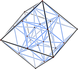
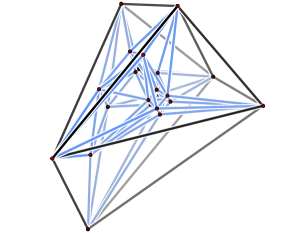
Fig. 4.3: The regular 24-cell and one other realisation from the family of Table 4.5.

Remark 4.14.

Clearly, not all possible realisations of the $24$-cell are contained in this $4$-parameter family. The $24$-cell in Table 4.5 is also a result of the construction and has no projective automorphisms.

4.5 Fatness of polytopes

The classification of $f$- and flag vectors for polytopes in dimension $d\geq 4$ is an important unsolved problem in polytope theory. See [Bay87], [Zie02] for some background on this problem and overviews of the known results.

Ziegler [Zie02] proposed to look at the following quantity (called the “fatness” of a polytope $P$) on the entries of these two vectors.

$$F(P):=\frac{f_{1}+f_{2}-20}{f_{0}-f_{3}-10}$$

where $(f_{0},f_{1},f_{2},f_{3})$ is the $f$-vector of any $4$-polytope different from the simplex (in [EKZ03] there is a slightly different definition). The fatness of polytopes produced from the $E$-construction applied to simple $4$-polytopes is bounded by $6$, cf. [EKZ03, p. 3]. Eppstein, Kuperberg, and Ziegler provided a polytope $Q$ resulting from a gluing of $600$-cells that has fatness around $5.073$ in the definition of [Zie02] (The $E$-construction also works for some non-simple polytopes, but all known examples don’t have a higher fatness). They also showed that for regular CW $3$-spheres fatness is unbounded. But they neither found polytopes with fatness higher than $5.073$ nor an upper bound on fatness for arbitrary polytopes.

For our family $E_{mn}$ we get according to the $f$-vector computation in (1):

$$F(E(C_{m}\times C_{n}))=\frac{12mn-20}{2mn+2m+2n-10}\longrightarrow 6$$

for $m,n\rightarrow\infty$. Thus for $m,n\geq 10$ our polytopes are “fatter” than the above mentioned example from [EKZ03]. As products of polygons are simple, our family of polytopes is “best possible” within this setting. However, Ziegler [Zie04] recently has constructed a class of polytopes (not “$E$-polytopes”) with fatness arbitrarily close to $9$ by considering projections of products of polygons to $\mathbb{R}^{4}$.

References

[Bay87]
Margaret M. Bayer, The extended -vectors of 4-polytopes, J. Comb.
Theory Ser. A 44 (1987), pp. 141–151.
[BB85]
Margaret M. Bayer and Louis J. Billera, Generalized Dehn-Sommerville
relations for polytopes, spheres, and partially ordered sets, Invent. Math.
79 (1985), pp. 143–157.
[Bok04]
Jürgen Bokowski, Computational Oriented Matroids,
Cambridge University Press, Cambridge, 2005, to appear
[BEK84] Jürgen Bokowski, Günter Ewald, and Peter
Kleinschmidt, On combinatorial and affine automorphisms of
polytopes, Israel J. Math. 47 (1984), pp. 123–130.
[EKZ03]
David Eppstein, Greg Kuperberg, and Günter M. Ziegler, Fat
4-polytopes and fatter 3-spheres, Discrete Geometry: in honour of W.
Kuperberg’s 60th birthday (A. Bezdek, ed.), Pure and Applied Mathematics. A
series of Monographs and Textbooks, vol. 253, Marcel Dekker, Inc., 2003,
pp. 239–265.
[GJ00]
Ewgenij Gawrilow and Michael Joswig, polymake: a framework for analyzing
convex polytopes, Polytopes—combinatorics and computation (Oberwolfach,
1997), DMV Sem., vol. 29, Birkhäuser, Basel, 2000, pp. 43–73.
[Gev02]
Gábor Geváy, On perfect polytopes, Beiträge Algebra
Geom. 43 (2002), pp. 243–259
[Gev04] , personal communication, October 2004
[Grü03]
Branko Grünbaum, Convex Polytopes, second ed., Graduate Texts in
Mathematics, vol. 221, Springer-Verlag, New York, 2003, Prepared and with a
preface by Volker Kaibel, Victor Klee and Günter M. Ziegler.
[Man71]
Peter Mani, Automorphismen von polyedrischen Graphen, Mathematische
Annalen 192 (1971), pp. 279–303.
[McM68]
Peter McMullen, Affinely and projectively regular polytopes, J. London
Math. Soc. 43 (1968), pp. 755–757.
[McM76] , Constructions for projectively unique polytopes, Discrete Math.
14 (1976), pp. 347–358.
[PZ04]
Andreas Paffenholz and Günter M. Ziegler, The -construction for
lattices, spheres and polytopes, Discrete Comp. Geom. (Billera Festschrift)
32 (2004), pp. 601–621.
[San00]
Francisco Santos, Triangulations with very few geometric
bistellar neighbors, Discrete Comp. Geom., 23 (2000),
pp. 15–33
[San03] , personal communication, April 2003.
[Sch11]
Issai Schur, Über Gruppen periodischer Substitutionen, Sber. preuss.
Akad. Wiss (1911), pp. 619–627.
[Zie95]
Günter M. Ziegler, Lectures on Polytopes, Graduate Texts in
Mathematics, vol. 152, Springer, New York, 1995.
[Zie02] , Face numbers of 4-polytopes and 3-spheres, Proceedings of the
ICM 2002, vol. III, 2002, pp. 625–634.
[Zie03] , personal communication, April 2003.
[Zie04] , Projected products of
polygons, Electron. Res. Announc. Amer. Math. Soc. 10
(2004), pp. 122–134.