Phylogenetic ideals and varieties for the general Markov model

Abstract

The general Markov model of the evolution of biological sequences along a tree leads to a parameterization of an algebraic variety. Understanding this variety and the polynomials, called phylogenetic invariants, which vanish on it, is a problem within the broader area of Algebraic Statistics. For an arbitrary trivalent tree, we determine the full ideal of invariants for the 2-state model, establishing a conjecture of Pachter-Sturmfels. For the $\kappa$-state model, we reduce the problem of determining a defining set of polynomials to that of determining a defining set for a 3-leaf tree. Along the way, we prove several new cases of a conjecture of Garcia-Stillman-Sturmfels on certain statistical models on star trees, and reduce their conjecture to a family of subcases.

,

1 Introduction

An important problem arising in modern biology is that of sequence-based phylogenetic inference. Suppose we obtain a collection of biological sequences, such as genomic DNA, from currently extant species, or taxa. Assuming these sequences evolved from a common ancestral sequence, how can we infer a tree that describes their evolutionary descent? The use of algebraic methods for this problem was first proposed in 1987 in independent works by Lake [14], and Cavender and Felsenstein [5]. Recently, Garcia, Stillman, and Sturmfels [10] initiated a more general algebraic study of statistical models, of which phylogenetic models are a particularly interesting example. In this new field, Algebraic Statistics, the viewpoints of algebraic geometry are central to investigations of probabilistic models arising in applied contexts.

In model-based phylogenetics, evolution is usually assumed to proceed along a binary tree from an ancestral sequence at the root of the tree, to sequences found in the taxa, which label the leaves of the tree. The $\kappa=4$ bases $A,C,G,T$ of which DNA is composed are viewed as states of random variables. Each site in the sequence might be assumed to evolve i.i.d., so that different sites can be viewed as trials of the same process. Probabilities of the various base substitutions along an edge of the tree can then be given by a Markov transition matrix along that edge. Additional biologically reasonable, or mathematically convenient, assumptions as to the form of these transition matrices are often imposed. The basic problem is to assume some model along these lines and use it to infer, from observations of DNA sequences only at the leaves, a tree topology that might describe their evolutionary descent. An excellent overview of the field of phylogenetics is provided by the recent volume of Felsenstein [9].

In the phylogenetics literature, a phylogenetic invariant for a particular model and tree is a polynomial that vanishes on all joint distributions of bases at the leaves that arise from the model, regardless of the values of the model parameters. In the terminology of algebraic geometry, the model and tree imply a parameterization of a dense subset of a variety, and phylogenetic invariants are the elements of the prime ideal defining that variety.

For applications, one might hope that the near-vanishing of phylogenetic invariants on observed frequencies of bases in DNA data could be used as a test of model-fit and/or tree topology. Although this idea remains undeveloped for practical use, phylogenetic invariants have already provided means for addressing more theoretical questions in phylogenetics, such as the nature of maximum likelihood points [6], and the identifiability of certain models [4].

In this paper we investigate the phylogenetic variety for the general Markov model of base substitution for an arbitrary tree, a detailed specification of which will be given in the next section. This model was also the focus of the related investigations [1, 2].

One main result is the proof of Conjecture 13 of Pachter and Sturmfels [16] on the ideal of phylogenetic invariants for the general Markov model in the case of $\kappa=2$ states: the invariants arising from all $3\times 3$ minors of ‘2-dimensional flattenings’ of an array along the edges of a binary $n$-taxon tree $T$ generate the full ideal. This is Theorem 4, which is stated more fully in Section 4 and proved in Section 8.

Figure 1: A 5-taxon tree

For an explicit example of this theorem, consider the 5-taxon tree of Figure 1. Then for the 2-state model, denote the states by 0 and 1. A $2\times 2\times 2\times 2\times 2$ tensor $P$ encodes the probabilities of various states at the leaves, where $P(i_{1},i_{2},i_{3},i_{4},i_{5})=p_{i_{1}i_{2}i_{3}i_{4}i_{5}}$ is the joint probability of observing state $i_{j}$ in the sequence at leaf $a_{j}$, $j=1,\dots,5$. Now $P$ has two natural flattenings according to the partitions of leaves produced by deleting an internal edge of the tree. The partitions, or splits, are $\{\{a_{1},a_{2}\},\{a_{3},a_{4},a_{5}\}\}$, and $\{\{a_{1},a_{2},a_{3}\},\{a_{4},a_{5}\}\}$, and the corresponding flattenings are

$$\begin{pmatrix}p_{00000}&p_{00001}&p_{00010}&p_{00011}&p_{00100}&p_{00101}&p_{00110}&p_{00111}\\ p_{01000}&p_{01001}&p_{01010}&p_{01011}&p_{01100}&p_{01101}&p_{01110}&p_{01111}\\ p_{10000}&p_{10001}&p_{10010}&p_{10011}&p_{10100}&p_{10101}&p_{10110}&p_{10111}\\ p_{11000}&p_{11001}&p_{11010}&p_{11011}&p_{11100}&p_{11101}&p_{11110}&p_{11111}\end{pmatrix}$$

and

$$\begin{pmatrix}p_{00000}&p_{00001}&p_{00010}&p_{00011}\\ p_{00100}&p_{00101}&p_{00110}&p_{00111}\\ p_{01000}&p_{01001}&p_{01010}&p_{01011}\\ p_{01100}&p_{01101}&p_{01110}&p_{01111}\\ p_{10000}&p_{10001}&p_{10010}&p_{10011}\\ p_{10100}&p_{10101}&p_{10110}&p_{10111}\\ p_{11000}&p_{11001}&p_{11010}&p_{11011}\\ p_{11100}&p_{11101}&p_{11110}&p_{11111}\end{pmatrix}.$$

The theorem states that the $3\times 3$ minors of these two matrices generate the prime ideal of all phylogenetic invariants for the 2-state general Markov model on this tree. In particular, this ideal has a natural set of generators that correspond to the splits, and therefore to specific topological features of the tree.

We note that this theorem provides the first determination of all phylogenetic invariants for an arbitrary binary tree for any non-group-based model. Sturmfels and Sullivant [19] solved the similar problem for group-based models, using the Hadamard conjugation ([12, 13, 8, 20]) to recognize the varieties as toric. While algebraic models intermediate to the group-based and general ones have been introduced recently [3, 7], our knowledge of them is less complete.

We also investigate the question of the explicit determination of the phylogenetic variety and ideal for larger $\kappa$. We show in Theorem 17 that if we have a set of polynomials whose zero set is the variety for the 3-taxon tree, then we can construct a set of polynomials whose zero set is the variety for any binary $n$-taxon tree. Similar to the conjecture of [16], our constructions involve ‘flattenings’, though both 2- and 3-dimensional ones are now needed, as might be expected from [1]. Thus the only remaining obstruction to our determination of a defining set of polynomials for the phylogenetic variety for any binary tree and any number of states $\kappa$ is the determination of a defining set for the 3-taxon tree variety.

In Conjecture 5 we suggest that the same construction yielding set-theoretic defining polynomials for the variety would yield generators of the full prime ideal vanishing on the variety, provided we begin with generators of the ideal for the 3-taxon tree. This is the analog for arbitrary $\kappa$ of the Pachter-Sturmfels conjecture.

Theorem 4, Theorem 17, and Conjecture 5, as well as the Sturmfels-Sullivant group-based result, can all be viewed as statements that the phylogenetic varieties and ideals arise from the ‘local structure’ of the tree. Exploiting this observation to provide better ways of characterizing the statistical support a data set might provide for specific local tree features would be interesting work for the future. In particular, invariants might provide a means of characterizing support for particular splits or tripartitions of the taxa.

Despite our primary focus on phylogenetic models, to prove Theorem 17 we must consider certain other statistical models on star trees. In Section 6, we therefore investigate models with a $\kappa$-state hidden variable associated to the internal node, and $l_{i}$-state observed variables associated to the $n$ leaves. Such models are of course interesting in applications outside of phylogenetics, as they are examples of rather common ‘mixture models’ in statistics. Following [10], they are termed hidden naive Bayes models.

Our work here focuses on such models in the case that for each $i$ the number of states $l_{i}$ is at least as large as the number of hidden states $\kappa$. Theorems 10 and 11 describe how set-theoretic and ideal-theoretic defining sets of the associated varieties can be deduced from set-theoretic and ideal-theoretic defining sets of the variety of the related model which has $\kappa$-state variables on each leaf.

As a consequence of this work on star tree models, in Corollary 14 we prove several cases of Conjecture 21 of [10], on ideal generators for the hidden naive Bayes model with $\kappa=2$. While one of these cases, for the 3-leaf tree, has been recently proved in [15], even for that case our argument is different, and perhaps more direct. Moreover, our work indicates that establishing the special cases mentioned in Conjecture 16 of this paper is sufficient to prove the full conjecture of [10].

Before obtaining these results, we begin with several background sections. In Section 2, we define the phylogenetic variety for the general Markov model through the natural parameterization arising from modeling molecular evolution along a tree $T$ by associating Markov matrices to each edge. In Section 3 we then give a more convenient parameterization of (a dense subset of) the cone over the phylogenetic variety, which associates an arbitrary $\kappa\times\kappa$ matrix to each edge of $T$, rather than a Markov matrix. Section 4 introduces flattenings of tensors along edges and vertices of trees, while Section 5 develops the relationship of a form of multiplication of tensors to the varieties under investigation. Subsequent sections contain our primary results.

Finally, we note that most of the results on phylogenetic trees in this paper hold not only for binary trees, but also under the weaker assumption that each vertex have valency at least three. An important exception is Theorem 4, where the binary assumption is critical to our proof.

2 Affine and Projective Phylogenetic Varieties

Let $T$ denote an $n$-taxon tree, by which we mean a tree with all internal vertices unlabeled and of valency at least 3, with $n$ leaves labeled by taxa $a_{1},\dots,a_{n}$. We will sometimes specify in addition that $T$ is binary (i.e., all internal vertices are trivalent), as this assumption is needed for some of our results, and is often the case of primary interest in phylogenetics.

Choosing as a root any vertex $r$ of $T$, either internal or a leaf, denote the rooted tree by $T^{r}$. Parameters for the $\kappa$-state general Markov model of sequence evolution on $T^{r}$ consist of a root distribution vector $\boldsymbol{\pi}_{r}=(\pi_{1},\pi_{2},\dots,\pi_{\kappa})$ with non-negative entries summing to 1, together with a $\kappa\times\kappa$ Markov matrix $M_{e}$, which has non-negative entries with each row summing to 1, for each of the $2n-3$ edges $e$ of $T^{r}$ directed away from $r$.

This models the evolution of biological sequences as follows. The $\kappa$ states $[\kappa]=\{1,2,\dots,\kappa\}$ correspond to the alphabet from which sequences are composed. The root $r$ represents the most recent common ancestor of the currently extant taxa, and other internal nodes of the tree represent most recent common ancestors of those taxa separated from the root by that node. The root distribution vector encodes the frequencies $\pi_{i}$ with which each state $i$ occurs in an ancestral sequence at $r$. The $(i,j)$-entry of a Markov matrix along a particular edge of $T$ directed away from $r$ is the conditional probability of state $i$ changing to state $j$ at any particular site in the sequence during evolution along that edge. Thus each site in a biological sequence is assumed to evolve independently, according to the same process (i.i.d.). Note the biological term ‘sequence’ as used here implies no mathematical structure other than a correspondence between sites based on ancestry; except for matching sites by common ancestry, the ordering of the sites within the sequences is irrelevant.

Suppose a rooted $n$-taxon tree $T^{r}$ has $|E|$ edges, so that for a binary tree $|E|=2n-3$. For the general Markov model of evolution along $T^{r}$ the parameter space $S$ can thus be identified with a subset of $[0,1]^{N}$, where $N=(\kappa-1)+|E|\kappa(\kappa-1)$.

Furthermore, there is a polynomial map $\phi_{r}:S\to[0,1]^{L}$, $L=\kappa^{n}$, giving the joint distribution of states in sequences at the leaves resulting from any parameter choice. We view points in $\phi_{r}(S)$ or $\mathbb{C}^{L}$ as $\kappa\times\cdots\times\kappa$ tensors, with the $i$th index referring to the state at leaf $a_{i}$. Indices thus typically range through $[\kappa]$, and a fixed ordering of the taxa is reflected in the ordering of indices of tensors. Assuming the model adequately reflects real molecular evolution, from biological sequence data we can estimate entries of $\phi_{r}(s)$, but usually have little or no direct information about the parameters $s$.

The map $\phi_{r}$ is explicitly given by $\phi_{r}(s)=P$, where

$$P(i_{1},\dots,i_{n})=\sum_{(b_{v})\in H}\left(\boldsymbol{\pi}_{r}(b_{r})\prod_{e}M_{e}(b_{s(e)},b_{f(e)})\right),$$ (1)

where the product is taken over all edges $e$ of $T^{r}$ directed away from $r$, edge $e$ has initial vertex $s(e)$ and final vertex $f(e)$ and associated Markov matrix $M_{e}$, and the sum is taken over the set

$$H=\{(b_{v})_{v\in Vert(T)}~{}|~{}b_{v}\in[\kappa]\text{ if $v\neq a_{j}$},\ b_{v}=i_{j}\text{ if $v=a_{j}$}\}\subset[\kappa]^{2n-2}.$$

Thus $H$ represents the set of all ‘histories’ consistent with the specified states at the leaves.

The map $\phi_{r}$ can also be defined inductively, using matrix algebra, by viewing the tree $T^{r}$ as built up from smaller trees by the addition of pairs of terminal edges, as we now explain. For this purpose, we first assume $T$ is binary.

A cherry of $T$ is a pair of distinct leaves $a_{i_{1}},a_{i_{2}}$ whose incident edges contain a common (internal) vertex of $T$. For $n\geq 3$, any binary $n$-taxon tree contains at least two cherries, and any rooted binary $n$-taxon tree contains at least one cherry in which neither taxon of the cherry is the root of the tree.

For $n\geq 3$ let $T^{r}_{n}=T^{r}$ denote a rooted binary $n$-taxon tree labeled by taxa $a_{1},\dots,a_{n}$. Choose a cherry of $T^{r}_{n}$ which does not contain the root $r$. Let $T^{r}_{n-1}$ denote the rooted binary $(n-1)$-taxon tree obtained by deleting the cherry and its two incident edges from $T_{n}^{r}$ and labeling as a new taxon, say $b$, the (formerly internal) common vertex of the incident edges.

Applying this definition recursively, we obtain from $T^{r}$ a sequence of rooted trees $T^{r}_{n},T^{r}_{n-1},\dots,T^{r}_{2}$, which of course may depend on some arbitrary choices of cherries. We assume such choices have been made and fixed.

The map $\phi_{r}$ described above can now be described inductively as follows:

A rooted $2$-taxon tree has only one edge $e$ directed away from $r$, so with parameters $\boldsymbol{\pi}_{r}$ and $M_{e}$,

$$\phi_{r}(\boldsymbol{\pi}_{r};M_{e})=\operatorname{diag}(\boldsymbol{\pi}_{r})M_{e},$$

where $\operatorname{diag}(\mathbf{v})$ denotes the square matrix with $\mathbf{v}$ on its main diagonal and zeros elsewhere.

To define $\phi_{r}$ for $T^{r}_{m}$, direct edges $e$ away from $r$ and suppose parameters

$$s=(\boldsymbol{\pi}_{r};\{M_{e}\})$$

for $T^{r}_{m}$ are given. Then one obtains parameters $\tilde{s}$ for $T^{r}_{m-1}$ by simply discarding from $s$ the two Markov matrices associated to the edges of $T^{r}_{m}$ not appearing in $T^{r}_{m-1}$. Inductively, we may assume $\tilde{\phi}_{r}:\tilde{S}\to[0,1]^{\kappa^{m-1}}$, the map giving the joint distribution of states at leaves for $T^{r}_{m-1}$ as a function of parameters on $T^{r}_{m-1}$, has been given. For convenience, we also assume that taxa of $T^{r}_{m}$ are $a_{1},a_{2},\dots,a_{m}$ and those of $T^{r}_{m-1}$ are $a_{1},a_{2},\dots,a_{m-2},b$, with the given orderings, and that $e_{1}$ and $e_{2}$ are the edges of $T^{r}_{m}$ containing $a_{m-1},a_{m}$ respectively.

Then $\phi_{r}(s)=P$, where $P$ is an $m$-dimensional tensor with 2-dimensional slices given by first letting $\tilde{P}=\tilde{\phi}_{r}(\tilde{s})$, $\mathbf{v}=\tilde{P}(i_{1},\dots,i_{m-2},\cdot)$ and setting

$$P(i_{1},\dots,i_{m-2},\cdot,\cdot)=M_{e_{1}}^{T}\operatorname{diag}(\mathbf{v})M_{e_{2}}.$$ (2)

One can check that this definition of $\phi_{r}$ agrees with our earlier one, and so is independent of the choice of cherries defining the sequence $T_{2}^{r},T_{3}^{r},\dots,T_{n}^{r}$.

This approach to an inductive definition of $\phi_{r}$ can be extended to the case of non-binary trees as follows. For an arbitrary tree $T^{r}$, let $\widetilde{T}^{r}$ denote any binary tree which resolves $T^{r}$, in the sense that $T^{r}$ can be obtained from $\widetilde{T}^{r}$ by contraction of some edges. Extend a choice of parameters $s$ on $T^{r}$ to parameters $\tilde{s}$ on $\widetilde{T}^{r}$ by assigning the identity matrix to those edges of $\widetilde{T}^{r}$ which are collapsed in $T^{r}$. Then since $\phi_{r}(s)=\tilde{\phi}_{r}(\tilde{s})$, the inductive definition for binary trees can be applied for $\widetilde{T}^{r}$.

Lemma 1

For any $n$-taxon tree $T$, the inductive definition of $\phi_{r}$ based on Eq. (2) and outlined above agrees with the definition in Eq. (1).

We also denote by $\phi_{r}$ the unique extension of this map to a polynomial map $\phi_{r}:\mathbb{C}^{N}\to\mathbb{C}^{L}$. The affine phylogenetic variety $V(T)$ for the general Markov model on $T$ is defined as the closure in $\mathbb{C}^{L}$ of the image of $\phi_{r}$. (Note that this closure may be taken using either the Zariski topology or the standard topology on $\mathbb{C}^{L}$, as the two closures will agree for the image of a polynomial map.) As has been shown elsewhere [17, 1], this definition is independent of the choice of the root $r$. $V(T)$ is irreducible, as it is the zero set of a prime ideal, the kernel of the map between polynomial rings associated to $\phi_{r}$.

Now one readily sees the image of $\phi_{r}$ lies on the hyperplane defined by the trivial phylogenetic invariant $\sum_{\mathbf{i}\in[\kappa]^{n}}P(\mathbf{i})-1=0$. It is therefore natural to pass to the projective phylogenetic variety in $\mathbb{P}^{L-1}$ by taking a projective closure. We denote this by $V(T)$ also, making clear by context whether the affine or projective version is meant.

The phylogenetic ideals of all polynomials vanishing on the affine phylogenetic variety or vanishing on the projective phylogenetic variety are of course closely related. Generators of the homogeneous ideal $\mathfrak{a}_{T}$ of the projective variety, together with the trivial invariant, generate the ideal of the affine variety. Conversely, any homogeneous polynomial in the ideal of the affine variety is in the homogeneous ideal of the projective variety. Thus identifying phylogenetic invariants for the general Markov model means identifying those polynomials vanishing on the projective phylogenetic variety.

3 Reparameterization

For any projective variety $V\subseteq\mathbb{P}^{m}$, let $CV\subseteq\mathbb{C}^{m+1}$ denote the cone over $V$, that is, the union of the lines represented by points in $V$. Equivalently, $CV$ is the affine variety defined by the same polynomials as $V$.

A dense subset of the cone $CV(T)$ admits a parameterization that will be more useful than the parameterization $\phi_{r}$ above. This new parameterization simplifies many arguments, since it allows matrices with any row sums to be associated to edges, and no longer requires a root distribution, or even a specification of a root.

Definition 2

Consider an $n$-taxon tree $T$ with $|E|$ edges. Let $U=\mathbb{C}^{K}$ with $K=|E|\kappa^{2}$. Choose any vertex of $T$ as a root, directing all edges of $T^{r}$ away from $r$. View $u\in\mathbb{C}^{K}$ as a $(2n-3)$-tuple of complex $\kappa\times\kappa$ matrices $M_{e}$, one for each edge $e$ of $T^{r}$.

Then, in the case that $T$ is binary, let $\psi:U\to\mathbb{C}^{L}$ be given inductively as follows, using the sequence of trees $T^{r}=T_{n}^{r},T_{n-1}^{r},\dots,T_{2}^{r}$ chosen in the discussion leading to Lemma 1:

If $n=2$, $\psi(u)=\psi(M_{e})=M_{e}$, so $\psi$ is the identity map.

If $n>2$, let $\tilde{\psi}:\tilde{U}\to\mathbb{C}^{\kappa^{n-1}}$ be the map associated to $T_{n-1}^{r}$. Then for $u\in U$, define $\tilde{u}\in\tilde{U}$ by omitting from $u$ the matrices associated to the edges $e_{1},e_{2}$ of $T_{n}^{r}$ not in $T_{n-1}^{r}$. Then $\psi(u)=P$, where $P$ is a $n$-dimensional tensor with 2-dimensional slices given by first letting $\tilde{P}=\tilde{\psi}(\tilde{u})$, $\mathbf{v}=\tilde{P}(i_{1},\dots,i_{n-2},\cdot)$ and setting

$$P(i_{1},\dots,i_{n-2},\cdot,\cdot)=M_{e_{1}}^{T}\operatorname{diag}(\mathbf{v})M_{e_{2}}.$$

For non-binary trees, modify this construction as indicated for Lemma 1.

As in Lemma 1, one sees that this map is independent of the choice of cherries determining the sequence $T_{2}^{r},T_{3}^{r},\dots,T_{n}^{r}$. Although $\psi$ apparently depends on the choice of $r$, one can further check that if $r$ is moved from one vertex of an edge $e$ to the other vertex, we need only transpose the matrix $M_{e}$ associated to that edge and the map is unchanged. Thus the map is independent of the choice of $r$, though our conception of how components of $\mathbb{C}^{K}$ are placed into matrices does depend on $r$. Indeed, all these observations follow from the observation that $\psi$ can also be defined by a formula like that in Eq. (1), but with the factor $\boldsymbol{\pi}_{r}(b_{r})$ omitted.

Proposition 3

The closure of $\psi(U)$ in $\mathbb{C}^{L}$ is the cone $CV(T)$ over the phylogenetic variety $V(T)$.

[Proof.] To see $\phi_{r}(S)\subseteq\psi(U)$, suppose $s=(\boldsymbol{\pi}_{r};\{M_{e}\})\in S$. Let $e_{0}$ be the one edge of $T_{2}^{r}$, and define $M_{e_{0}}^{\prime}=\operatorname{diag}(\boldsymbol{\pi}_{r})M_{e_{0}}$. With $u=(M_{e_{0}}^{\prime},\{M_{e}\}_{e\neq e_{0}})$, we find that $\phi_{r}(s)=\psi(u)$. Thus $V(T)\subseteq\overline{\psi(U)}$. Furthermore $\psi(U)$ is a cone, since if $u=(\{M_{e}\})\in U$ and $\lambda\in\mathbb{C}$, by picking any particular edge $e_{0}$ of $T$ and defining $u^{\prime}\in U$ to be identical to $u$ but with $\lambda M_{e_{0}}$ replacing $M_{e_{0}}$, then $\psi(u^{\prime})=\lambda\psi(u)$. Thus $CV(T)\subseteq\overline{\psi(U)}$.

We next show there is a non-empty open, and therefore dense, subset of $U$ whose image under $\psi$ lies in the cone over $\phi_{r}(S)$, and hence in $CV(T)$. This will imply $\overline{\psi(U)}\subseteq CV(T)$.

For simplicity of exposition, assume $T^{r}$ is binary.

First, if $n=2$, then $\phi_{r}(S)$ certainly contains those 2-dimensional arrays whose entries add to 1 and none of whose row sums are 0. Now the subset of $U$ on which all row sums of $M_{e}(=u)$ are non-zero and the total sum of the entries of $M_{e}(=u)$ is non-zero is an open set. The points in the image under $\psi$ of this open set lie in the cone over $\phi_{r}(S)$.

Proceeding inductively, let $e_{1}$,$e_{2}$ be the edges of $T_{m}^{r}$ which are not in $T_{m-1}^{r}$, and $e_{3}$ the third edge meeting them. We may also suppose $r$ does not lie at the common vertex of $e_{1},e_{2},e_{3}$. Now there is an open $\mathcal{O}_{1}\subset U$ such that for points $u\in\mathcal{O}_{1}$, $M_{e_{1}}$ and $M_{e_{2}}$ have all row sums non-zero. Letting $D_{i}$ be the invertible diagonal matrix constructed from the row sums of $M_{e_{i}}$, we may write

$$M_{e_{i}}=D_{i}M^{\prime}_{e_{i}},\ \ i=1,2,$$

where $M^{\prime}_{e_{i}}$ has rows summing to 1. Let $M_{e_{3}}^{\prime}=M_{e_{3}}D_{1}D_{2}$. Then for any $u\in\mathcal{O}_{1}$, we define a new $u^{\prime}\in\mathcal{O}_{1}$ as

$$u^{\prime}=(\{M_{e}\}_{e\notin\{e_{1},e_{2},e_{3}\}},M^{\prime}_{e_{1}},M^{\prime}_{e_{2}},M^{\prime}_{e_{3}}),$$

so that $\psi(u^{\prime})=\psi(u)$. Note that $\omega:\mathcal{O}_{1}\to\mathcal{O}_{1}$ mapping $u\mapsto u^{\prime}$ is given by rational functions.

Let $\tilde{\psi}:\tilde{U}\to\mathbb{C}^{\kappa^{m-1}}$ and $\tilde{\phi}_{r}:\tilde{S}\to\mathbb{C}^{\kappa^{m-1}}$ be the parameterizations associated to $T^{r}_{m-1}$. Then by induction there is a non-empty open $\tilde{\mathcal{O}}\subset\tilde{U}$ such that the image of all points in $\tilde{\mathcal{O}}$ under $\tilde{\psi}$ lie in the cone over $\tilde{\phi}_{r}(\tilde{S})$. Then $\mathcal{O}=\omega^{-1}(\tilde{\mathcal{O}}\times\mathbb{C}^{2\kappa^{2}})$ is a non-empty open subset of $U$, and the image of any point of $\mathcal{O}$ under $\psi$ lies in the cone over $\phi_{r}(S)$.

If $T^{r}$ is not binary, slight modifications can be made to the above argument to obtain the result. ∎

While the definition of $\psi$ has introduced many unnecessary parameters, in the sense that the dimension of the image is much smaller than the dimension of the parameter space, it offers us the advantage of dropping inconvenient requirements — that row sums of vectors and matrices be 1 — that arose from the original probabilistic setting of the general Markov model.

4 Flattenings and phylogenetic invariants

To describe the set of phylogenetic invariants we are concerned with, we require the notion of flattening a tensor $P\in\mathbb{\mathbb{C}}^{\kappa^{n}}$ according to an $n$-taxon tree $T$.

Let $e$ be an edge of $T$. Then $e$ induces a split of the taxa according to the connected components of $T\setminus\{e\}$. By reordering the indices in $P$ if necessary, we may assume the split is $\left\{\{a_{1},\dots,a_{k}\},\ \{a_{k+1},\dots,a_{n}\}\right\}$. The flattening of $P$ on $e$ is the $\kappa^{k}\times\kappa^{n-k}$ matrix $F=Flat_{e}(P)$ defined as follows: Fix any ordering of $J_{1}=[\kappa]^{k}$ and $J_{2}=[\kappa]^{n-k}$, and for $u\in J_{1}$, $v\in J_{2}$, let $F(u,v)=P(u_{1},\dots,u_{k},v_{1},\dots,v_{n-k})$.

If the tensor $P=\phi_{r}(s)$ gives the joint distribution of states for some parameter choice for the general Markov model on $T$, then $Flat_{e}(P)$ can be thought of as a joint distribution for a related graphical model with less complicated structure: For a tree with at least 3 leaves, choose the root $r$ to be at one vertex of the edge $e$, and imagine at $r$ a $\kappa$-state hidden variable. The possible joint states at the taxa $a_{1},\dots,a_{k}$ are viewed as a single $\kappa^{k}$-state observed variable. Similarly, the joint states at the taxa $a_{k+1},\dots,a_{n}$ are described through a single $\kappa^{n-k}$-state variable. We thus have a “coarser” graphical model with one hidden $\kappa$-state internal node and two descendent nodes with $\kappa^{k}$ and $\kappa^{n-k}$ states, respectively, as depicted in Figure 2. The flattening of $P$ simply prevents one from examining the finer structure in the joint distribution array that arises from the branching of $T$ on either side of $e$.

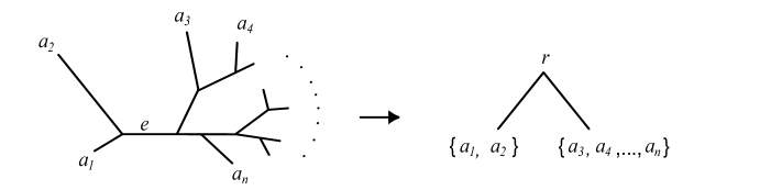
Figure 2: Flattening on an edge $e$

From this interpretation one readily sees that for any $P\in\phi_{r}(S)$, $Flat_{e}(P)$ has rank at most $\kappa$. Indeed, for the coarser graphical model, the joint distribution matrix must have the form

$$Flat_{e}(P)=M_{1}^{T}\operatorname{diag}(\pi_{r})M_{2}$$

where $M_{1}$ and $M_{2}$ are $\kappa\times\kappa^{k}$ and $\kappa\times\kappa^{n-k}$ Markov matrices.

As a result, all $(\kappa+1)\times(\kappa+1)$ minors of $Flat_{e}(P)$ must vanish. As is classically known, such minors generate the full prime ideal of polynomials vanishing on matrices of rank $\leq\kappa$, and thus generate all invariants associated to the coarser model. For the original model on $T$, these minors therefore give phylogenetic invariants, which we call edge invariants associated to the edge $e$.

We denote by $\mathcal{F}_{edge}(T)$ the set of all $(\kappa+1)\times(\kappa+1)$ minors of all flattenings of a $\kappa\times\cdots\times\kappa$ tensor of $\kappa^{n}$ indeterminates on edges of $T$. Of course the choice of ordering of rows and columns in the flattening introduces factors of $\pm 1$, but as our goal is to determine ideal generators, we may ignore this issue.

In Section 8 we will establish the following, which was conjectured in [16].

Theorem 4

For $\kappa=2$ and any number of taxa $n$, the phylogenetic ideal $\mathfrak{a}_{T}$ for the general Markov model on a binary $n$-taxon tree $T$ is generated by $\mathcal{F}_{edge}(T)$, the $3\times 3$ minors of all edge flattenings of a $2\times\cdots\times 2$ tensor of indeterminates.

However, for larger $\kappa$ it is not enough to consider only 2-dimensional edge flattenings (i.e., flattenings to matrices) to obtain generators of the phylogenetic ideal. This can be seen already for the $3$-taxon tree. In this case, $\mathcal{F}_{edge}(T)$ is empty, but for any $\kappa>2$ the phylogenetic ideal contains polynomials of degree $\kappa+1$ (see [1]; for $\kappa=3$ see also [10]). Thus we need at least to consider flattenings of $P$ at internal nodes of $T$ producing 3-dimensional tensors.

More specifically, consider a trivalent internal vertex $v$ of a tree $T$, contained in edges $e_{1},e_{2},e_{3}$. Then $v$ induces a tripartition of the taxa according to the connected components of $T\setminus\{v,e_{1},e_{2},e_{3}\}$. By reordering the indices in $P$ if necessary, we may assume the tripartition is

$$\left\{\{a_{1},\dots,a_{k}\},\ \{a_{k+1},\dots,a_{k+l}\},\ \{a_{k+l+1},\dots,a_{n}\}\right\}.$$

Then a flattening of $P$ at $v$ is a $\kappa^{k}\times\kappa^{l}\times\kappa^{n-k-l}$ array $F=Flat_{v}(P)$ defined as follows: Fix an ordering of $J_{1}=[\kappa]^{k}$, $J_{2}=[\kappa]^{l}$, and $J_{3}=[\kappa]^{n-k-l}$ , and for $u\in J_{1}$, $v\in J_{2}$, $w\in J_{3}$, let $F(u,v,w)=P(u_{1},\dots,u_{k},v_{1},\dots,v_{l},w_{1},\dots,w_{n-k-l})$.

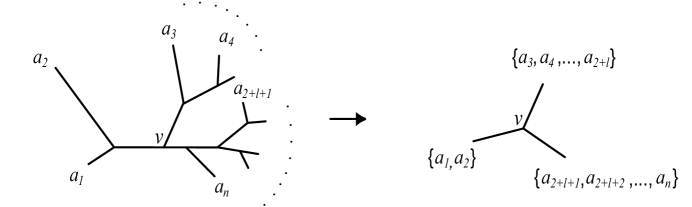
Figure 3: Flattening at a vertex $v$

As illustrated in Figure 3, we think of this flattening as producing a joint distribution array associated to a graphical model with one hidden $\kappa$-state internal node and three descendent nodes with $\kappa^{k}$, $\kappa^{l}$, and $\kappa^{n-k-l}$ states, respectively. Similar to flattenings on edges, a flattening at an internal node ignores the finer structure in the joint distribution array that arises from the branching of $T$ in the three directions leading away from $v$.

An ideal is associated to such a graphical model (1 hidden $\kappa$-state ancestral node, 3 descendent nodes), and so to the flattening at a vertex. While we will investigate such ideals further in Section 6, already we can formulate a natural extension of the conjecture of [16].

Conjecture 5

For any $\kappa$ and any number of taxa $n$, the phylogenetic ideal $\mathfrak{a}_{T}$ for the general Markov model on a binary $n$-taxon tree $T$ is the sum of the ideals associated to the flattenings of $P$ at vertices of $T$.

That this conjecture is identical to Theorem 4 when $\kappa=2$ follows from work of Landsberg and Manivel [15]. They show that in this special case the ideal associated to a vertex flattening is the sum of those associated to the edge flattenings on the three edges containing the vertex. (The Landsberg-Manivel result is a special case of a conjecture in [10]. We will give a new and simpler proof of this case, and several additional cases, as Corollary 14.)

Of course the notion of flattening at a vertex can be extended in a straightforward way for vertices of valence $>3$, and the conjecture formulated for non-binary trees as well. The extended conjecture for non-binary trees remains open even for $\kappa=2$.

Although we will primarily need to refer to the 2- and 3-dimensional flattenings of a tensor $P$ on an edge or at a vertex of a tree $T$, the notion naturally extends to flattenings based on any partition of the set of labels (taxa) associated to the indices of $P$. For instance, an $n$-dimensional $\kappa\times\cdots\times\kappa$ tensor $P$ with associated labels $a_{1},\dots,a_{n}$ can be flattened according to the partition $\left\{\{a_{1}\},\dots,\{a_{n-2}\},\{a_{n-1},a_{n}\}\right\}$ to give an $(n-1)$-dimensional $\kappa\times\cdots\times\kappa\times\kappa^{2}$ tensor. We use such a flattening, where $a_{n-1},a_{n}$ are in a cherry, in Section 8. Flattenings according to arbitrary bipartitions also appear in Section 6.

5 The algebra of tensors, trees, and parameters

In this section we define binary operations on trees, model parameters on trees, and tensors. These operations, all denoted by the same symbol ‘$*$’, exhibit relationships that will make them useful in later sections.

Tensors: If $Q$ and $R$ are $m$- and $n$-dimensional tensors of ‘matching size $\kappa$’ in the last and first index respectively, then we define an $l=(m+n-2)$-dimensional tensor $Q*R$ by

$$(Q*R)(i_{1},\dots i_{l})=\sum_{j=1}^{\kappa}Q(i_{1},\dots,i_{m-1},j)R(j,i_{m},\dots,i_{l}).$$

For $m=n=2$, this is of course just matrix multiplication.

More generally, if the $p$th index of $Q$ and the $q$th index of $R$ both run through $[\kappa]$, we may define $Q*_{p,q}R$ by a similar sum. However, to keep our notation less cumbersome, we will generally try to express products using the last and first indices.

Trees: Suppose $T^{\prime}$ is a tree with taxa $a_{1},a_{2},\dots,a_{m}$, and $T^{\prime\prime}$ is a tree with taxa $b_{1},b_{2},\dots,b_{n}$. Then by $T^{\prime}*T^{\prime\prime}$ we mean the $(m+n-2)$-taxon tree with taxa $a_{1},\dots,a_{m-1},b_{2},\dots,b_{n}$ obtained by first identifying the vertices $a_{m}$ and $b_{1}$, and then deleting this vertex, replacing the two edges it lies in with a single conjoined edge, as illustrated in Figure 4.

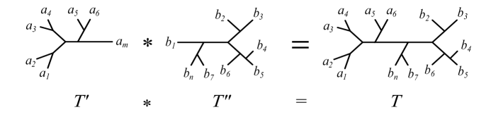
Figure 4: The $*$ operation on trees

Parameters: Consider trees $T^{\prime}$, $T^{\prime\prime}$, and $T=T^{\prime}*T^{\prime\prime}$ with $m$, $n$, and $m+n-2$ taxa. Then from Section 3 we have the parameterizations

$$\psi^{\prime} :U^{\prime}\to\mathbb{C}^{\kappa^{m}},$$

$$\psi^{\prime\prime} :U^{\prime\prime}\to\mathbb{C}^{\kappa^{n}},$$

$$\psi :U\to\mathbb{C}^{\kappa^{m+n-2}},$$

of the cones over the associated phylogenetic varieties.

To impose directions on the edges of the trees for notational purposes, root $T^{\prime}$ and $T$ at $a_{1}$, and $T^{\prime\prime}$ at $b_{1}$. Then for $u^{\prime}\in U^{\prime}$, $u^{\prime\prime}\in U^{\prime\prime}$, we define $u^{\prime}*u^{\prime\prime}\in U$ by retaining for each edge of $T$ except the conjoined one the matrix associated to the edge in either $u^{\prime}$ or $u^{\prime\prime}$, and for the conjoined edge using the product of the matrices in $u^{\prime}$ and $u^{\prime\prime}$ associated to its parts.

One readily sees that these three definitions imply the following.

Lemma 6

$\psi(u^{\prime}*u^{\prime\prime})=\psi^{\prime}(u^{\prime})*\psi^{\prime\prime}(u^{\prime\prime})$.

Lemma 7

If $T=T^{\prime}*T^{\prime\prime}$, then $CV(T)=\overline{CV(T^{\prime})*CV(T^{\prime\prime})}.$

[Proof.] It is clear that

$$U=U^{\prime}*U^{\prime\prime}=\{u^{\prime}*u^{\prime\prime}~{}|~{}u^{\prime}\in U^{\prime},\ u^{\prime\prime}\in U^{\prime\prime}\}.$$

Thus by Lemma 6,

$$CV(T)=\overline{\psi(U)}=\overline{\psi^{\prime}(U^{\prime})*\psi^{\prime\prime}(U^{\prime\prime})}=\overline{CV(T^{\prime})*CV(T^{\prime\prime})}.$$

∎

This result will be strengthened in Corollary 21.

In the special case when $T^{\prime\prime}$ is a 2-taxon tree, $T^{\prime}*T^{\prime\prime}$ is isomorphic to $T^{\prime}$. Then $u^{\prime\prime}=\psi(u^{\prime\prime})$ is simply a $\kappa\times\kappa$ matrix. Informally, one can think of $\psi^{\prime}(u^{\prime})*\psi^{\prime\prime}(u^{\prime\prime})$ as the result of ‘extending’ the edge of $T^{\prime}$ terminating at $a_{m}$ and associating to the edge extension the matrix $u^{\prime\prime}$.

Considering invertible matrices $u^{\prime\prime}$, we get an action of $GL(\kappa,\mathbb{C})$ on both $U^{\prime}$ and $\psi^{\prime}(U^{\prime})$. Thus $GL(\kappa,\mathbb{C})$ acts on the closure, $CV(T^{\prime})$, as well. Viewing the action described here as operating in ‘the last index’ of a tensor in $V_{T^{\prime}}$, we similarly have an action in the other indices. These actions of $GL(\kappa,\mathbb{C})$ are of course just restrictions of the natural actions of that group on the set of all $\kappa\times\cdots\times\kappa$ tensors: For $j=1,\dots,n$, the ‘$j$th index’ action is defined by $P\mapsto P*_{j,1}A$ for $A\in GL(\kappa,\mathbb{C})$.

6 Models on star trees

In this section, we step back from the phylogenetic tree setting, and consider in more depth the hidden naive Bayes models of [10]. Most of our results will be needed for application to phylogenetic varieties. However, we develop this material in slightly greater generality than we need for phylogenetic applications, and so obtain partial results on a conjecture of [10] as well.

The graphical models of this section are based on a star tree, as in Figure 5, with one internal vertex $r$, connected by edges to $n$ leaves $a_{1},a_{2},\dots,a_{n}$. A hidden random variable associated to $r$ has $\kappa$ possible states, with probability distribution given by a vector $\boldsymbol{\pi}_{r}$. Each leaf $a_{i}$ has associated to it a random variable with $l_{i}$ states, and Markov matrices $M_{i}$ of size $\kappa\times l_{i}$ give conditional probabilities of observing the various states at $a_{i}$ given the state at $r$.

Figure 5: Graphical depiction of a hidden naive Bayes model

As in the phylogenetic situation, such a model defines a projective variety, the closure of the set of joint distributions of observations at the leaves arising from this parameterization. We denote this variety by $V(\kappa;l_{1},l_{2},\dots,l_{n})$, and the homogeneous ideal defining it by $\mathfrak{a}(\kappa;l_{1},l_{2},\dots,l_{n})$.

As pointed out in [10], the variety $V(\kappa;l_{1},l_{2},\dots,l_{n})$ can be viewed more geometrically as the $\kappa$-secant variety of the Segre product $\mathbb{P}^{l_{1}-1}\times\mathbb{P}^{l_{2}-1}\times\dots\times\mathbb{P}^{l_{n}-1}$. Here ‘$\kappa$-secant variety’ means the closure of the union of the $(\kappa-1)$-dimensional affine spaces spanned by collections of $\kappa$ points on the original variety, so, for instance, the 2-secant variety arises from points on secant lines.

Note that $V(\kappa;\kappa,\kappa,\kappa)=V(T_{3})$, the phylogenetic variety for a $\kappa$-state, 3-taxon tree. The varieties $V(\kappa;\kappa^{k},\kappa^{l},\kappa^{n-k-l})$, with $k,l,n-k-l\geq 1$, are the ones that arose in Section 4, in the discussion of flattenings of tensors at vertices of phylogenetic trees. Moreover, flattenings on edges involve $V(\kappa;\kappa^{k},\kappa^{n-k}$), the variety of rank $\kappa$ matrices of size $\kappa^{k}\times\kappa^{n-k}$, which is well understood classically.

Our first goals are to show Theorems 10 and 11: Given a set $\mathcal{F}$ of polynomials set-theoretically (respectively, ideal-theoretically) defining $V(\kappa;\kappa,\kappa,\dots,\kappa)$ for the $n$-leaf star tree, then for any $l_{i}\geq\kappa$ we can explicitly construct polynomials set-theoretically (respectively, ideal-theoretically) defining $V(\kappa;l_{1},l_{2},\dots,l_{n})$.

Previous to these theorems, we know of only one general result concerning defining polynomials of $V(\kappa;l_{1},l_{2},\dots,l_{n})$: When $\kappa=2$, for any number of leaves, [15] gives a natural set of polynomials defining the variety as a set.

For our application to phylogenetic trees, the assumption that internal nodes are trivalent means only the case $n=3$ is needed. We therefore summarize known results on $V(\kappa;\kappa,\kappa,\kappa)=V(T_{3})$ for small $\kappa$.

For $\kappa=2$, as noted in [10, 1, 15], $V(T_{3})=\mathbb{P}^{7}$, and so $\{0\}$ is the full prime ideal defining the variety.

For $\kappa=3$, a generating set $\mathcal{F}$ for the prime ideal may be taken to be the 27 quartic polynomials in [10], first found in [18] but also obtained from the construction in [1].

For $\kappa\geq 4$, finding an explicit set $\mathcal{F}$ that even set-theoretically defines the variety is still an open problem. However, any polynomial vanishing on the variety must be of degree at least $\kappa+1$.

When $\kappa=4$, all degree 5 polynomials vanishing on the variety form an explicitly-known 1728-dimensional vector space. This dimension is computed in [11, 15], and an explicit construction for general $\kappa$ is given in [1] that produces a spanning set when $\kappa=4$. Moreover, off another explicitly-known variety, the vanishing of these polynomials does distinguish points of $V(T_{3})$. However, an explicit degree 9 polynomial is known which vanishes on $V(4;3,3,3)$ (see [10] for a statement, or [18] for the construction), and from this polynomial one can obtain degree 9 polynomials vanishing on $V(4;4,4,4)=V(T_{3})$ by evaluation on $3\times 3\times 3$ subarrays of a $4\times 4\times 4$ tensor. By consideration of the multidegrees of each monomial term in its many variables, one can show that these degree 9 polynomials cannot be generated by the degree 5 ones.

We also note that if $\phi$ is the parameterization arising from the general Markov model on $T_{3}$, then for all $\kappa\geq 2$ the image of $\phi$ is strictly smaller than its closure $V(T_{3})$. This is pointed out in Section 9 of [1], but in the terminology of [18] is simply the statement that ‘rank $\kappa$’ is a strictly stronger statement than ‘border rank $\kappa$’ for $\kappa\times\kappa\times\kappa$ tensors.

By modifying the approach of Section 3, it is possible to parameterize a dense subset of the cone $CV(\kappa;l_{1},l_{2},\dots,l_{n})$ using parameters which are arbitrary matrices. We leave the details to the reader, but denote this parameterization by $\psi_{\kappa;l_{1},\dots,l_{n}}$, where

$$\psi_{\kappa;l_{1},\dots,l_{n}}:U_{\kappa;l_{1},\dots,l_{n}}\to\mathbb{C}^{L},\ \ U_{\kappa;l_{1},\dots,l_{n}}=\mathbb{C}^{\kappa(l_{1}+\cdots+l_{n})},\ L=l_{1}l_{2}\cdots l_{n},$$

and if $P=\psi(M_{1},M_{2},\dots,M_{n})$ then

$$P(i_{1},\dots,i_{n})=\sum_{k=1}^{\kappa}\prod_{j=1}^{n}M_{j}(k,i_{j}).$$

Here $M_{j}\in M(\kappa,l_{j},\mathbb{C})$, the set of complex $\kappa\times l_{j}$ matrices.

In order to relate $V(\kappa;l_{1},l_{2},\dots,l_{n})$ to $V(\kappa;\kappa,\kappa,\dots,\kappa)$ we need the following lemma. It can be interpreted as describing the effect of extending one edge of the star tree, and associating a (non-square) matrix to that extension, as was explained at the end of Section 5.

Lemma 8

Let $P\in CV(\kappa;l_{1},l_{2},\dots,l_{n})$ and let $A\in M(l_{n},l^{\prime}_{n},\mathbb{C})$. Then $A$ defines a map $CV(\kappa;l_{1},l_{2},\dots,l_{n})\to CV(\kappa;l_{1},l_{2},\dots,l^{\prime}_{n})$ by $P\mapsto P*A$. Furthermore,

1. If $rank(A)=l_{n}^{\prime}$, then $CV(\kappa;l_{1},l_{2},\dots,l_{n})*A$ is dense in
   $CV(\kappa;l_{1},l_{2},\dots,l^{\prime}_{n})$.

2. If $\kappa\leq l_{n}$ then $CV(\kappa;l_{1},l_{2},\dots,l_{n})*M(l_{n},l^{\prime}_{n},\mathbb{C})$ is dense in
   $CV(\kappa;l_{1},l_{2},\dots,l^{\prime}_{n})$.

[Proof.] Suppose first that $P=\psi_{\kappa;l_{1},\dots,l_{n}}(M_{1},M_{2},\dots,M_{n})$, with complex $\kappa\times l_{i}$ matrix parameters $M_{i}$, $i=1,2,\dots,n$ associated to the $n$ edges of $T$ directed away from the internal node. Then

$$P*A=\psi_{\kappa;l_{1},\dots,l_{n-1},l_{n}^{\prime}}(M_{1},M_{2},\dots,M_{n-1},M_{n}A),$$

hence $P*A\in CV(\kappa;l_{1},l_{2},\dots,l^{\prime}_{n})$. Since $P*A\in CV(\kappa;l_{1},l_{2},\dots,l^{\prime}_{n})$ for $P$ in a dense subset of $CV(\kappa;l_{1},l_{2},\dots,l_{n})$, it follows that $P*A\in CV(\kappa;l_{1},l_{2},\dots,l^{\prime}_{n})$ for all $P\in CV(\kappa;l_{1},l_{2},\dots,l_{n})$.

Now suppose $\operatorname{rank}(A)=l^{\prime}_{n}$. Then as $M_{n}$ ranges through all $\kappa\times l_{n}$ complex matrices, $M_{n}A$ ranges through all $\kappa\times l_{n}^{\prime}$ complex matrices. Thus

$$\psi_{\kappa;l_{1},\dots,l_{n}}(U_{\kappa;l_{1},\dots,l_{n}})*A=\psi_{\kappa;l_{1},\dots,l_{n-1},l^{\prime}_{n}}(U_{\kappa;l_{1},\dots,l^{\prime}_{n}}),$$

and so a subset of $CV(\kappa;l_{1},\dots,l_{n})*A$ is dense in $CV(\kappa;l_{1},\dots,l^{\prime}_{n})$.

Finally suppose $\kappa\leq l_{n}$. Then as $M_{n}$ ranges through all $\kappa\times l_{n}$ complex matrices and $A$ through all $l_{n}\times l_{n}^{\prime}$ matrices, $M_{n}A$ ranges through all $\kappa\times l_{n}^{\prime}$ complex matrices. Thus

$$\psi_{\kappa;l_{1},\dots,l_{n}}(U_{\kappa;l_{1},\dots,l_{n}})*M(l_{n},l^{\prime}_{n},\mathbb{C})=\psi_{\kappa;l_{1},\dots,l_{n-1},l^{\prime}_{n}}(U_{\kappa;l_{1},\dots,l^{\prime}_{n}}).$$

Therefore a subset of $CV(\kappa;l_{1},\dots,l_{n})*M(l_{n},l^{\prime}_{n},\mathbb{C})$ is dense in
$CV(\kappa;l_{1},\dots,l^{\prime}_{n})$. ∎

Remark 9

For non-zero $P$ and $A$ as in the proof, it is possible for $P*A$ to be a zero tensor. Thus while the above lemma could be formulated in terms of a rational map between the underlying projective varieties, it is slightly easier for us to consider a polynomial map on the cones.

By permuting indices Lemma 8 can be applied in any index, not just the last. As shorthand, we will refer to this as letting an $l_{k}\times l_{k}^{\prime}$ matrix ‘act in the $k$th index.’ By considering only invertible $l_{k}\times l_{k}$ matrices, we have a group action of $GL(l_{k},\mathbb{C})$ in the $k$th index, and so an action of $GL(l_{1},\mathbb{C})\times\cdots\times GL(l_{n},\mathbb{C})$ on $V(\kappa;l_{1},\dots,l_{n})$. While this group action underlies the dimension computations of [15], our work will emphasize the utility of non-square and non-invertible matrices as well.

Theorem 10

Consider an $n$-leaf star tree. Suppose $l_{1},l_{2},\dots,l_{n}\geq\kappa$. Let $\mathcal{F}$ be any set of polynomials whose zero set is $V(\kappa;\kappa,\kappa,\dots,\kappa)$. For $k=1,2,\dots,n$, let $Z_{k}=(z_{ij}^{k})$ be $l_{k}\times\kappa$ matrices of indeterminates. For an $l_{1}\times l_{2}\times\dots\times l_{n}$ tensor $P$ of indeterminates, let $\tilde{P}$ be the $\kappa\times\kappa\times\dots\times\kappa$ tensor that results from letting each $Z_{k}$ act formally in the $k$th index of $P$. Let $\tilde{\mathcal{F}}$ denote the set of polynomials in the entries of $P$ obtained from those in $\mathcal{F}$ by substituting into them the entries of $\tilde{P}$, expressing the results as polynomials in the $z_{ij}^{k}$, and then extracting the coefficients. Let $\mathcal{F}_{edge}$ denote the set of $(\kappa+1)\times(\kappa+1)$ minors of the $n$ flattenings of $P$ on edges of the star tree. Finally, let $\mathcal{F}(\kappa;l_{1},l_{2},\dots,l_{n})=\tilde{\mathcal{F}}\cup\mathcal{F}_{edge}$.

Then $\mathcal{F}(\kappa;l_{1},l_{2},\dots,l_{n})$ defines $V(\kappa;l_{1},l_{2},\dots,l_{n})$ set-theoretically.

[Proof.] We first observe that all polynomials in $\mathcal{F}(\kappa;l_{1},l_{2},\dots,l_{n})$ vanish on the cone $CV(\kappa;l_{1},l_{2},\dots,l_{n})$: Polynomials in $\mathcal{F}_{edge}$ must vanish there, since the model has $\kappa$ states at the internal node, so all 2-dimensional flattenings on edges must have rank $\leq\kappa$ on the parameterized subset of the variety, and hence on the whole variety. Polynomials in $\tilde{\mathcal{F}}$ must vanish there, since for all assignments of values to the $z_{ij}^{k}$, if $P\in CV(\kappa,l_{1},\dots,l_{n})$ then, by Lemma 8, $\tilde{P}\in CV(\kappa;\kappa,\dots,\kappa)$.

Now suppose all polynomials in $\mathcal{F}(\kappa;l_{1},l_{2},\dots,l_{n})$ vanish on a tensor $P_{0}\in\mathbb{C}^{l_{1}l_{2}\cdots l_{n}}$. Then, flattening $P_{0}$ on the edge of the tree leading to $a_{n}$ gives a matrix of rank $l\leq\kappa$, so we can write

$$P_{0}=Q^{\prime}_{0}*B_{n}^{\prime}$$

where $Q_{0}^{\prime}$ is an $l_{1}\times l_{2}\times\dots\times l_{n-1}\times l$ tensor and $B_{n}^{\prime}$ is an $l\times l_{n}$ matrix. Construct a $\kappa\times l_{n}$ matrix $B_{n}$ of rank $\kappa$ by augmenting $B_{n}^{\prime}$ with additional rows. Similarly augment $Q_{0}^{\prime}$ with additional zero entries to obtain an $l_{1}\times l_{2}\times\dots\times l_{n-1}\times\kappa$ tensor $Q_{0}$ with $P_{0}=Q_{0}*B_{n}$. Now there exists an $l_{n}\times\kappa$ matrix $A_{n}$ so that $B_{n}A_{n}=I$, the identity matrix. Thus $P_{0}*A_{n}*B_{n}=Q_{0}*B_{n}*A_{n}*B_{n}=Q_{0}*I*B_{n}=P_{0}$.

Proceeding similarly for the other taxa, we obtain matrices $A_{k}$, $B_{k}$ such that

$$(P_{0}*_{k,1}A_{k})*_{k,1}B_{k}=P_{0}*_{k,1}(A_{k}*B_{k})=P_{0}.$$

By simultaneously letting each $A_{k}$ act in the $k$th index of $P_{0}$, we obtain a $\kappa\times\kappa\times\dots\times\kappa$ tensor $\tilde{P}_{0}$. Because all polynomials in $\tilde{\mathcal{F}}$ vanish on $P_{0}$, all polynomials in $\mathcal{F}$ vanish on $\tilde{P}_{0}$. Thus by our choice of $\mathcal{F}$, $\tilde{P}_{0}\in CV(\kappa;\kappa,\kappa,\dots,\kappa)$. Since, by repeated applications of Lemma 8, letting each $B_{k}$ act in the $k$th index maps $CV(\kappa;\kappa,\kappa,\dots,\kappa)$ to $CV(\kappa;l_{1},l_{2},\dots,l_{n})$, and maps $\tilde{P}_{0}$ to $P_{0}$, we see $P_{0}\in CV(\kappa;l_{1},l_{2},\dots,l_{n})$. ∎

We now state an ideal-theoretic version of this result.

Theorem 11

Suppose $l_{1},l_{2},\dots,l_{n}\geq\kappa$, and $\mathcal{F}$ is a set of polynomials generating $\mathfrak{a}(\kappa;\kappa,\kappa,\dots,\kappa)$. Then the set $\mathcal{F}(\kappa;l_{1},l_{2},\dots,l_{n})$ constructed from $\mathcal{F}$ as in Theorem 10 generates $\mathfrak{a}(\kappa;l_{1},l_{2},\dots,l_{n})$.

Since the key argument in the proof of Theorem 11 will be used again in Section 8, we present it as a lemma.

Lemma 12

Let $V_{1}$ and $V_{2}$ be subvarieties of $\mathbb{C}^{nm_{1}}$ and $\mathbb{C}^{nm_{2}}$, respectively, with $m_{1}\leq m_{2}$, such that, when points are written as $n\times m_{1}$ and $n\times m_{2}$ matrices,

$$V_{1}=V_{1}*M(m_{1},m_{1},\mathbb{C}),$$

and

$$V_{2}=\overline{V_{1}*M(m_{1},m_{2},\mathbb{C})}.$$

Let $\mathfrak{a}_{i}$ denote the ideal of all polynomials vanishing on $V_{i}$.

Then $\mathfrak{a}_{2}$ is generated by the $(m_{1}+1)\times(m_{1}+1)$ minors of an $n\times m_{2}$ matrix $P$ of indeterminates, together with all polynomials of the form $f(P*A)$, where $f\in\mathfrak{a}_{1}$ and $A\in M(m_{2},m_{1},\mathbb{C})$.

[Proof.] Let $\mathfrak{b}$ denote the ideal generated by the $(m_{1}+1)\times(m_{1}+1)$ minors, together with the polynomials $f(P*A)$ described above.

First we show $\mathfrak{a}_{2}\supseteq\mathfrak{b}$. It is enough to show the specified generators of $\mathfrak{b}$ vanish on $V_{1}*M(m_{1},m_{2},\mathbb{C})$. Since all points in this set are matrices of rank at most $m_{1}$, the specified minors vanish there. To see the $f(P*A)$ vanish there, consider a point $Q_{0}*B$ where $Q_{0}\in V_{1}$, $B\in M(m_{1},m_{2},\mathbb{C})$. Then $Q_{0}*B*A\in V_{1}$ since $B*A\in M(m_{1},m_{1},\mathbb{C})$. Thus $f(P*A)$ vanishes at $Q_{0}*B$.

Our argument that $\mathfrak{a}_{2}\subseteq\mathfrak{b}$ is more involved.

Note $GL(m_{2},\mathbb{C})$ acts on $V_{1}*M(m_{1},m_{2},\mathbb{C})$, and hence on $V_{2}$ as well. Consider the degree $m$ homogeneous component $\mathfrak{a}_{2}^{(m)}$ of $\mathfrak{a}_{2}$. Then the $GL(m_{2},\mathbb{C})$-action on $V_{2}$ gives a representation of $GL(m_{2},\mathbb{C})$ on $\mathfrak{a}_{2}^{(m)}$, in which $C\in GL(m_{2},\mathbb{C})$ maps the polynomial $g(P)\mapsto g(P*C)$. Since $GL(m_{2},\mathbb{C})$ is reductive, this representation decomposes into a sum of irreducible ones. Consider now one of the irreducible subspaces, $W$. It will be enough to show that $W\subseteq\mathfrak{b}$.

Consider any non-zero polynomial $g(P)\in W$. Let $Q$ denote a $n\times m_{1}$ matrix of indeterminates. Then for any $B\in M(m_{1},m_{2},\mathbb{C})$, the polynomial $g_{B}(Q)=g(Q*B)$ vanishes on $V_{1}$, since $Q_{0}\mapsto Q_{0}*B$ maps $V_{1}$ to $V_{2}$. Thus $g_{B}\in\mathfrak{a}_{1}$.

Suppose first that for all $B\in M(m_{1},m_{2},\mathbb{C})$ the polynomial $g_{B}(Q)$ is identically zero. Then $g$ must vanish on all $n\times m_{2}$ matrices of rank at most $m_{1}$, since any such matrix can be written as $Q_{0}*B$ for some complex matrices $Q_{0}\in M(n,m_{1},\mathbb{C})$, $B\in M(m_{1},m_{2},\mathbb{C})$, and then $g(Q_{0}*B)=g_{B}(Q_{0})=0$. Thus if all $g_{B}$ are identically zero, then $g$ is in the ideal generated by $(m_{1}+1)\times(m_{1}+1)$ minors of $P$, and hence $g\in\mathfrak{b}$.

Suppose, then, that for some $B$ the polynomial $g_{B}$ is not identically zero. Let $D\in M(m_{2},m_{1},\mathbb{C})$ be chosen so that $h(P)=g_{B}(P*D)$ is a non-zero polynomial. Such a $D$ must exist since $m_{1}\leq m_{2}$. (For instance, $D$ may be taken so that its first $m_{1}$ rows form an identity and the remaining rows are zero.) Then $h(P)=g(P*DB)$, where $DB$ is a complex $m_{2}\times m_{2}$ matrix that is generally not invertible.

Nonetheless, the irreducibility of $W$ implies that $h(P)\in W$. This is simply because $W$ is closed in $\mathfrak{a}_{2}^{(m)}$, and so must contain the closure of the orbit of $g$ under $GL(m_{2},\mathbb{C})$, and this closure contains $g(P*DB)$.

Now since $g(P)\in W$, $h(P)=g_{B}(P*D)\in W$, and $g_{B}\in\mathfrak{a}_{1}$, the irreducibility of $W$ implies $g(P)$ is in the span of polynomials of the form $f(P*A)$ where $f\in\mathfrak{a}_{1}$ and $A\in M(m_{2},m_{1},\mathbb{C})$. Thus in this case as well, $g\in\mathfrak{b}$. ∎

[Proof.][Proof of Theorem 11] Let $\mathfrak{a}=\mathfrak{a}(\kappa;l_{1},\dots,l_{n})$, and let $\mathfrak{b}$ be the ideal generated by $\mathcal{F}(\kappa;l_{1},\dots,l_{n})$, the set defined in Theorem 10. Note that $\mathfrak{b}$ is equivalently described as generated by $\mathcal{F}_{edge}\cup\tilde{\tilde{\mathcal{F}}}$, where $\tilde{\tilde{\mathcal{F}}}$ denotes the set of all polynomials of the form $f(\tilde{P})$ where $f\in\mathcal{F}$ and $\tilde{P}$ is obtained from a tensor $P$ of indeterminates by the action of numerical matrices $Z_{k}\in M(l_{k},\kappa,\mathbb{C})$ in each index $k$.

That $\mathfrak{a}\supseteq\mathfrak{b}$ was shown in the proof of Theorem 10. To establish $\mathfrak{a}\subseteq\mathfrak{b}$. we proceed by induction on the number of indices $k$ such that $l_{k}>\kappa$, the base case of zero being trivial.

If at least one such $l_{k}>\kappa$ exists, we may assume $l_{n}>\kappa$. Then let $V_{1}=CV(\kappa;l_{1},\dots,l_{n-1},\kappa)$ and $V_{2}=CV(\kappa;l_{1},l_{2},\dots,l_{n})$. We view points on $V_{1}$ and $V_{2}$ as $l_{1}\cdots l_{n-1}\times\kappa$ and $l_{1}\cdots l_{n-1}\times l_{n}$ matrices, respectively, by flattening on the edge of the star tree leading to the $n$th leaf. Using Lemma 8 we see that $V_{1}*M(\kappa,\kappa,\mathbb{C})=V_{1}$ and, since $l_{n}>\kappa$, that $V_{2}=\overline{V_{1}*M(\kappa,l_{n})}$. Therefore we may apply Lemma 12, and obtain that $\mathfrak{a}$ is generated by the $(\kappa+1)\times(\kappa+1)$ minors of the flattening of $P$ on the edge to the $n$th leaf, together with all polynomials $f(P*A)$ where $f\in\mathfrak{a}(\kappa;l_{1},\dots,l_{n-1},\kappa)$ and $A\in M(l_{n},\kappa,\mathbb{C})$. We thus need only show such $f(P*A)$ are in $\mathfrak{b}$.

Now by induction, $\mathfrak{a}(\kappa;l_{1},\dots,l_{n-1},\kappa)$ is generated by $(\kappa+1)\times(\kappa+1)$ minors of edge flattenings of an $l_{1}\times\cdots\times l_{n-1}\times\kappa$ tensor $Q$ of indeterminates, together with polynomials of the form $h(\tilde{Q})$, where $h\in\mathfrak{a}(\kappa;\kappa,\dots,\kappa)$ and $\tilde{Q}$ is a $\kappa\times\cdots\times\kappa$ tensor obtained from $Q$ by letting elements of $M(l_{i},\kappa,\mathbb{C})$ (respectively $M(\kappa,\kappa,\mathbb{C})$) act on $Q$ in the $i$th index for each $i\neq n$ (respectively $i=n$). We may thus assume $f$ itself has one of these forms.

In the first case, where $f\in\mathfrak{a}(\kappa;l_{1},\dots,l_{n-1},\kappa)$ is a minor of an edge flattening for the model, we see $f$ vanishes on all tensors $Q$ that have rank at most $\kappa$ when flattened on a certain edge $e$ not leading to the $n$th leaf. But if $P$ is an $l_{1}\times\cdots\times l_{n}$ tensor with $\operatorname{rank}(Flat_{e}(P))\leq\kappa$, then $\operatorname{rank}(Flat_{e}(P*A))\leq\kappa$ as well, for all $A\in M(l_{n},\kappa,\mathbb{C})$. Thus $f(P*A)$ vanishes on all tensors such that $\operatorname{rank}(Flat_{e}(P))\leq\kappa$, and so $f(P*A)$ is in the ideal generated by $(\kappa+1)\times(\kappa+1)$ minors from edge flattenings of $P$.

In the second case, where $f=h(\tilde{Q})$, we find $f(P*A)=h(\tilde{P})$ where $\tilde{P}$ is obtained from $P$ by letting elements of $M(l_{i},\kappa,\mathbb{C})$ act on $P$ in the $i$th index for each $i$, and $h$ vanishes on $V(\kappa;\kappa,\cdots,\kappa)$.

Thus in either case $f(P*A)\in\mathfrak{b}$. ∎

Remark 13

It is natural to ask whether a smaller set of polynomials than the set described above — namely, those constructed by evaluation of polynomials in $\mathcal{F}$ on all $\kappa\times\cdots\times\kappa$ subarrays of a $l_{1}\times\cdots\times l_{n}$ array of indeterminates — is sufficient to define the variety $V(\kappa;l_{1},\dots,l_{n})$. Indeed, Lemma 15 below shows it does in the special case $\kappa=2$, assuming elements of $\mathcal{F}$ have a special form.

However, in general this subset does not even define the variety set-theoretically. To see this, consider the $3\times 3\times 4$ tensor

$$P=e_{1}\otimes e_{1}\otimes f_{1}+e_{2}\otimes e_{2}\otimes f_{2}+e_{3}\otimes e_{3}\otimes f_{3}+e_{1}\otimes e_{2}\otimes f_{4},$$

where the $e_{i}$ are the standard basis vectors for $\mathbb{C}^{3}$ and the $f_{i}$ the standard basis vectors for $\mathbb{C}^{4}$. That all $3\times 3\times 3$ subarrays of $P$ are in $V(3;3,3,3)$ is clear from the form of $P$. One can verify that $P\notin V(3;3,3,4)$ by checking the non-vanishing at $P$ of some of the polynomials constructed in Theorem 11.

As a corollary to Theorem 11, we prove several cases of Conjecture 21 in [10] on the ideals $\mathfrak{a}(2;l_{1},\dots,l_{n})$. We note the $n=3$ case was first proved in [15] by invoking sophisticated methods of Weyman [21].

Corollary 14

For $n\leq 5$, the ideal $\mathfrak{a}(2;l_{1},\dots,l_{n})$ associated to the hidden naive Bayes model with a 2-state hidden variable and $n$ observed variables with $l_{1},\dots,l_{n}$ states, is generated by the $3\times 3$ minors of all 2-dimensional flattenings associated to bipartitions of the observed variables.

[Proof.] Since there are no polynomials vanishing on $V(2;2,2,2)=\mathbb{P}^{7}$, by Theorem 11 the set of polynomials vanishing on $V(2;l_{1},l_{2},l_{3})$ is generated by edge invariants.

By calculations of [10], the statement holds for the two cases $V(2;2,2,2,2)$ and $V(2;2,2,2,2,2)$. The corollary then follows from Lemma 15 below. ∎

Lemma 15

Suppose, for the $n$-leaf star tree, that the ideal $\mathfrak{a}(2;2,\dots,2)$ is generated by the $3\times 3$ minors of all 2-dimensional flattenings of $2\times\cdots\times 2$ tensors according to bipartitions of the observed variables. Then $\mathfrak{a}(2;l_{1},\dots,l_{n})$ is generated by the $3\times 3$ minors of all 2-dimensional flattenings of $l_{1}\times\cdots\times l_{n}$ tensors according to bipartitions of the observed variables.

[Proof.] By Theorem 11, $\mathfrak{a}(2;l_{1},\dots,l_{n})$ is generated by all $3\times 3$ minors of edge flattenings of an $l_{1}\times\cdots\times l_{n}$ tensor of indeterminates $P$, together with all $3\times 3$ minors of all 2-dimensional flattenings of all $\tilde{P}$, where $\tilde{P}$ denotes a $2\times\cdots\times 2$ tensor obtained from $P$ by an action in each index $i$ by matrices $A_{i}\in M(l_{i},2,\mathbb{C})$. One readily sees such flattenings of $\tilde{P}$ can be expressed as $\tilde{F}=B_{1}*F*B_{2}$, where $F$ is the corresponding flattening of $P$ and the $B_{j}$ are matrices depending on the $A_{i}$. But then the $3\times 3$ minors of such a flattening of $\tilde{P}$ will be zero provided $F$ has rank $\leq 2$. Thus these polynomials are in the ideal $\mathfrak{b}$ generated by $3\times 3$ minors of flattenings of $P$. Therefore $\mathfrak{a}(2;l_{1},\dots,l_{n})\subseteq\mathfrak{b}$.

That $\mathfrak{a}(2;l_{1},\dots,l_{n})\supseteq\mathfrak{b}$ is clear. ∎

A proof of the full Conjecture 21 of [10] will therefore follow from the following special cases:

Conjecture 16

(Garcia,Stillman,Sturmfels) The ideal $\mathfrak{a}(2;2,2,\dots,2)$, that is, the ideal associated to the hidden naive Bayes model with a 2-state hidden variable and $n$ 2-state observed variables, is generated by the $3\times 3$ minors of all 2-dimensional flattenings arising from bipartitions of the observed variables.

7 Set-theoretic description of the phylogenetic variety: arbitrary $\kappa$.

For the remainder of this paper, we return to the consideration of models on phylogenetic trees. We first establish a set-theoretic result that provides some evidence for Conjecture 5, for arbitrary $\kappa$.

Theorem 17

For an $n$-taxon tree $T$, let $\mathcal{F}(T)$ be the union of all sets of polynomials $\mathcal{F}(\kappa;l_{1},l_{2},\dots l_{n})$, defined as in Theorem 10, associated to flattenings at nodes of $T$. Then the zero set of $\mathcal{F}(T)$ is the phylogenetic variety $V(T)$.

More informally, in conjunction with Theorem 10 this means that from polynomials whose zero set is $V(\kappa;\kappa,\dots,\kappa)$ one can explicitly construct polynomials whose zero set is $V(T)$ for any $n$-taxon tree $T$.

In particular, knowledge of set-theoretic defining polynomials for $V(T_{3})$ is sufficient to give set-theoretic defining polynomials for $V(T)$ for any binary tree $T$. Thus while one might naively view the case of $V(T_{3})$ as the simplest, in fact it is the only remaining barrier to the determination of polynomials defining the binary $n$-taxon variety, for any $n$. In the cases $\kappa=2,3$ where such defining polynomials are known, we thus obtain the following.

Corollary 18

For $\kappa=2$ or 3, and any binary tree $T$, explicit polynomials set-theoretically defining V(T) can be given.

Note that for $\kappa=2$ a stronger result is provided by Theorem 4, to be proved in Section 8.

For the remainder of this section let $V_{Flat}(T)$ denote the zero set of $\mathcal{F}(T)$. Our proof of Theorem 17 will follow several lemmas. The first is an analog for $V_{Flat}(T)$ of Lemma 7.

Lemma 19

Let $T^{\prime}$ and $T^{\prime\prime}$ be $n$-taxon and $m$-taxon trees, with $T=T^{\prime}*T^{\prime\prime}$. If $Q\in CV_{Flat}(T^{\prime})$ and $R\in CV_{Flat}(T^{\prime\prime})$, then $Q*R\in CV_{Flat}(T)$.

[Proof.] Consider any internal node $v$ of $T$, which we may assume arises from an internal node of $T^{\prime}$. We assume $v$ is trivalent; straight-forward modifications to our argument give the general case.

Flattening $Q$ at $v$, the resulting tensor lies on $CV(\kappa;\kappa^{n_{1}},\kappa^{n_{2}},\kappa^{n_{3}})$, with $n_{3}=n-n_{1}-n_{2}$, where we assume taxon $a_{n}$ of $T^{\prime}$ (where taxon $b_{1}$ of $T^{\prime\prime}$ is to be joined) is included in the last index of the flattening. Then the flattening of $Q*R$ at $v$ is obtained from the flattening of $Q$ at $v$ by an action in the third index by a matrix $R^{\prime}$ whose entries are determined by those of $R$. By Lemma 8 the flattening of $Q*R$ at $v$ lies in $CV(\kappa;\kappa^{n_{1}},\kappa^{n_{2}},\kappa^{n_{3}+m-2})$.

Thus $Q*R\in CV_{Flat}(T)$. ∎

We also need a converse to this lemma.

Lemma 20

Let $T^{\prime}$ and $T^{\prime\prime}$ be $n$-taxon and $m$-taxon trees, with $T=T^{\prime}*T^{\prime\prime}$. Then if $P\in CV_{Flat}(T)$, there exist $Q\in CV_{Flat}(T^{\prime})$ and $R\in CV_{Flat}(T^{\prime\prime})$ with $P=Q*R$.

[Proof.]

Let $e$ be the edge of $T$ formed by conjoining edges of $T^{\prime}$ and $T^{\prime\prime}$. Since any $P\in CV_{Flat}(T)$ satisfies the edge invariants for $e$, we may flatten it on $e$ to obtain a $\kappa^{n-1}\times\kappa^{m-1}$ matrix of rank $l\leq\kappa$, and write

$$P=Q*R,$$

where $Q$ and $R$ are $n$- and $m$-dimensional tensors, respectively, with all indices running through $[\kappa]$. We may further assume the non-zero $Q_{k}=Q(\cdot,\cdots,\cdot,k)$ are linearly independent, as are the non-zero $R_{k}=R(k,\cdot,\cdots,\cdot)$, and that $Q_{k},R_{k}$ are non-zero only for $k=1,\dots,l\leq\kappa$.

We next show $Q\in CV_{Flat}(T^{\prime})$. First observe that since the non-zero $R_{k}$ are independent, if we write them as row vectors, there is a $\kappa^{m-1}\times\kappa$ matrix $A$ so that $R_{k}A=\mathbf{e}_{k}$ for all $k\leq l$. Now supposing the taxa of $T^{\prime}$ and $T^{\prime\prime}$ are $a_{1},\dots,a_{n}$ and $b_{1},\dots,b_{m}$, respectively, flatten $P$ according to the partition $\left\{\{a_{1}\},\dots,\{a_{n-1}\},\{b_{2},\dots,b_{m}\}\right\}$ to an $n$-dimensional $\kappa\times\cdots\times\kappa\times\kappa^{m-1}$ tensor $F$. Letting $R^{\prime}$ denote the $\kappa\times\kappa^{m-1}$ flattened form of $R$ with rows $R_{k}$, we have $F=Q*R^{\prime}$. Thus $F*A=Q*R^{\prime}*A=Q$. (Note that $A$ does not act in a single index of $P$ here, but does act in a single index of the flattening $F$.) It is now straightforward to see that any flattening of $Q$ at an internal vertex of $T^{\prime}$ is obtained from a flattening of $P$ at a vertex of $T$, followed by an action in one of the resulting indices of a matrix determined by $A$. Thus by the definition of $\mathcal{F}(T)$, $Q$ will satisfy all polynomials in $\mathcal{F}(T^{\prime})$.

Similarly, $R\in CV_{Flat}(T^{\prime\prime})$. ∎

[Proof.][Proof of Theorem 17] We already know that $V_{Flat}(T)\supseteq V(T)$.

The proof that $V_{Flat}(T)=V(T)$ proceeds by induction on the number $n$ of taxa. The cases of $n=2,3$ hold by the definition of $\mathcal{F}(T)$.

For simplicity, we first consider a binary tree $T=T_{n}$,with $n\geq 4$ taxa. Picking a cherry of $T$, let $T_{n-1}$ and $T_{3}$ be such that $T=T_{n-1}*T_{3}$. Suppose $P\in CV_{Flat}(T)$. By Lemma 20, we have $P=Q*R$, for $Q\in CV_{Flat}(T_{n-1})$ and $R\in CV_{Flat}(T_{3})$. This, in combination with Lemma 19, means the map

$$\mu:CV_{Flat}(T_{n-1})\times CV_{Flat}(T_{3})\to CV_{Flat}(T_{n})$$

defined by $(Q,R)\mapsto Q*R$ is surjective.

Denote the parameterizations of the cones over the phylogenetic varieties for $T_{k}$ by $\psi_{k}:U_{k}\to\mathbb{C}^{L_{k}}$. With the map $\alpha:U_{n-1}\times U_{3}\to U_{n}$ defined by $\alpha(u_{n-1},u_{3})=u_{n-1}*u_{3},$ the diagram

$$\begin{CD}U_{n-1}\times U_{3}@>{\psi_{n-1}\times\psi_{3}}>{}>CV_{Flat}(T_{n-1})\times CV_{Flat}(T_{3})\\ @V{\alpha}V{}V@V{\mu}V{}V\\ U_{n}@>{\psi_{n}}>{}>CV_{Flat}(T)\end{CD}$$

commutes, by Lemma 6.

Now $\alpha$ and $\mu$ are surjective, and by the inductive hypothesis the image of $\psi_{n-1}\times\psi_{3}$ is dense in $CV_{Flat}(T_{n-1})\times CV_{Flat}(T_{3})$, so the image of $\psi_{n}$ is dense in $CV_{Flat}(T)$. Thus $V_{Flat}(T)=V(T)$.

If $T$ is not binary, the above argument may be modified by replacing the decomposition $T=T_{n-1}*T_{3}$ by $T=T_{n-k+1}*T_{k+1}$ where $T_{k+1}$ is a star tree with $k+1$ leaves and $T_{n-k+1}$ has $n-k+1$ leaves, if necessary. ∎

Theorem 17 and the preceding lemmas yield the following strengthening of Lemma 7.

Corollary 21

If $T=T^{\prime}*T^{\prime\prime}$, then $CV(T)=CV(T^{\prime})*CV(T^{\prime\prime})$.

8 The phylogenetic ideal: Binary $T$ and $\kappa=2$.

We now prove Theorem 4, and thus assume $T$ is a binary tree and $\kappa=2$.

Our arguments will use in several ways the fact (see Section 6) that for $\kappa=2$ the variety $V(T_{3})$ fills its ambient space: $V(T_{3})=\mathbb{P}^{7}.$ Note, however, that for $\kappa>2$, $V(T_{3})\subsetneq\mathbb{P}^{\kappa^{3}-1}$, and so the approach here cannot be successfully modified in a simple way.

The first use of this special fact is to note that for our chosen $\kappa$, $V(2;2,2,2)=V(T_{3})=\mathbb{P}^{7}$ means the set $\mathcal{F}$ defining $V(T_{3})$ is $\{0\}$. Thus the set $\mathcal{F}(T_{n})$ of the set-theoretic result Theorem 17 is the set of edge invariants. While our goal is to show $\mathcal{F}(T_{n})$ generates the full ideal vanishing on $V(T_{n})$, we will not, in fact, appeal to Theorem 17 to do so.

The second use of $V(T_{3})=\mathbb{P}^{7}$ is more subtle. Recall that regardless of $\kappa$, there are actions of $GL(\kappa,\mathbb{C})$ on $V(T_{n})$ in each index. However, in the case $\kappa=2$, the special nature of $V(T_{3})$ gives us actions of $GL(4,\mathbb{C})$ on $V(T_{n})$ via the cherries of $T_{n}$. This is really the key point in our argument, as it underlies the application of Lemma 12. Nonetheless, this action is in some respect an ‘unnatural’ consequence of $\kappa=2$. The following lemma provides a more careful statement of the special structure we use.

Lemma 22

Let $T_{n}$ denote a binary $n$-taxon tree, labeled so that taxa $a_{n-1}$ and $a_{n}$ form a cherry. Write $T_{n}=T_{n-1}*T_{3}$, where $a_{n-1},a_{n}$ are taxa on $T_{3}$. Let $e$ denote the edge of $T_{n}$ formed from conjoining edge $\tilde{e}$ of $T_{n-1}$ and the appropriate edge of $T_{3}$. View points in $CV(T_{n})$ and $CV(T_{n-1})$ as $2^{n-2}\times 4$ and $2^{n-2}\times 2$ matrices by flattening them on the edges $e$ and $\tilde{e}$, respectively. Then

$$CV(T_{n})=\overline{CV(T_{n-1})*M(2,4,\mathbb{C})}$$

and

$$CV(T_{n-1})=CV(T_{n-1})*M(2,2,\mathbb{C}).$$

[Proof.] The first claim is simply Lemma 7 applied to $T_{n-1}$ and $T_{3}$, combined with the observation that $CV(T_{3})=\mathbb{C}^{8}$ flattens to give $M(2,4,\mathbb{C})$. (Note that by Corollary 21, we could also remove the closure symbol here.)

For the second claim, apply the same argument to $T_{n-1}$ and $T_{2}$, observing that $CV(T_{2})=M(2,2,\mathbb{C})$. ∎

[Proof.][Proof of Theorem 4] We proceed by induction on the number $n$ of taxa for $T_{n}$, with the cases of $n=2,3$ known.

Let $\mathfrak{a}=\mathfrak{a}_{T}$ denote the ideal vanishing on $CV(T)$, and $\mathfrak{b}$ the ideal generated by $\mathcal{F}_{edge}(T)$. That $\mathfrak{a}\supseteq\mathfrak{b}$ has been discussed already; we must show the opposite inclusion.

With $T_{n}=T$, choose a cherry so that $T_{n}=T_{n-1}*T_{3}$, with notation as in Lemma 22. By that lemma, we may apply Lemma 12 with $V_{1}=CV(T_{n-1})$ and $V_{2}=CV(T_{n})$. We thus find $\mathfrak{a}$ is generated by the $3\times 3$ minors of the edge flattening $Flat_{e}(P)$ on the conjoined edge $e$ of an $n$-dimensional tensor of indeterminates $P$, together with all polynomials of the form $g(P)=f(Flat_{e}(P)*B)$ where $f(Q)$ vanishes on $CV(T_{n-1})$, $Q$ is a $(n-1)$-dimensional tensor of indeterminates, and $B\in M(4,2,\mathbb{C})$.

Now, by induction, the ideal of such $f$ is generated by $3\times 3$ minors of $Flat_{e^{\prime}}(Q)$ as $e^{\prime}$ ranges through edges of $T_{n-1}$. Consider one such minor, say $f_{0}$, obtained from the flattening on an edge $e_{0}$ of $T_{n-1}$. We may assume $e_{0}\neq\tilde{e}$, since otherwise there are no $3\times 3$ minors. It will be enough to show $f_{0}(Flat_{e}(P)*B)\in\mathfrak{b}$.

We claim that $f_{0}(Flat_{e}(P)*B)$ vanishes on all $P$ that have rank at most 2 when flattened on the edge $e_{0}$ in $T_{n}$. For such a $P$, since $Flat_{e_{0}}(P)$ is $2^{m}\times 2^{n-m}$, there is an expression $P=P_{1}*P_{2}$, where $P_{1}$ is an $(m+1)$-dimensional $2\times\cdots\times 2$ tensor, and $P_{2}$ an $(n-m+1)$-dimensional $2\times\cdots\times 2$ tensor. Then writing $P$ and $P_{2}$ as $2\times\cdots\times 2\times 4$ tensors by flattening to combine the taxa $a_{n-1},a_{n}$, we have $P*B=P_{1}*(P_{2}*B)$. This shows $P*B$ also has rank at most 2 when flattened on $e_{0}$, and so $f_{0}$ vanishes on it, as claimed.

But since $f_{0}(Flat_{e}(P)*B)$ vanishes on all $P$ of rank at most 2 when flattened on $e_{0}$, it is contained in the ideal generated by $3\times 3$ minors of flattenings on $e_{0}$. Thus it is in $\mathfrak{b}$. ∎

References

- [1] Elizabeth S. Allman and John A. Rhodes. Phylogenetic invariants for the general Markov model of sequence mutation. Math. Biosci., 186:113–144, 2003.
- [2] Elizabeth S. Allman and John A. Rhodes. Quartets and parameter recovery for the general Markov model of sequence mutation. App. Math. Res. Express (AMRX), 2004:4:107–131, 2004.
- [3] Elizabeth S. Allman and John A. Rhodes. Phylogenetic invariants for stationary base composition. J. Symbolic Comp., 41(2):138–150, 2006.
- [4] Elizabeth S. Allman and John A. Rhodes. The identifiability of tree topology for phylogenetic models, including covarion and mixture models. J. Comput. Biol., 13(5):1101–1113, 2006. arXiv:q-bio.PE/0511009.
- [5] James A. Cavender and Joseph Felsenstein. Invariants of phylogenies in a simple case with discrete states. J. of Class., 4:57–71, 1987.
- [6] B. Chor, M. D. Hendy, B. R. Holland, and D. Penny. Multiple maxima of likelihood in phylogenetic trees: an analytic approach. Mol. Bio. and Evol., 17:1529–1541, 2000.
- [7] Nicholas Eriksson, Kristian Ranestad, Bernd Sturmfels, and Seth Sullivant. Phylogenetic algebraic geometry. In Projective Varieties with Unexpected Properties; Siena, Italy, pages 237–256, Berlin, 2004. de Gruyter. arXiv:math.AG/0407033.
- [8] Steven N. Evans and T. P. Speed. Invariants of some probability models used in phylogenetic inference. Ann. Statist., 21(1):355–377, 1993.
- [9] Joseph Felsenstein. Inferring Phylogenies. Sinauer Associates, Sunderland, MA, 2004.
- [10] Luis David Garcia, Michael Stillman, and Bernd Sturmfels. Algebraic geometry of Bayesian networks. J. Symbolic Comp., 39:331–355, 2005. arXiv:math.AG/0301255.
- [11] Thomas R. Hagedorn. A combinatorial approach to determining phylogenetic invariants for the general model, 2000. Technical report, Centre de recherches math matiques.
- [12] Michael D. Hendy. The relationship between simple evolutionary tree models and observable sequence data. Systematic Zoology, 38:310–321, 1989.
- [13] Michael D. Hendy and David Penny. A framework for the quantitative study of evolutionary trees. Systematic Zoology, 38:297–309, 1989.
- [14] J.A. Lake. A rate independent technique for analysis of nucleic acid sequences: Evolutionary parsimony. Mol. Bio. Evol., 4(2):167–191, 1987.
- [15] J. M. Landsberg and L. Manivel. On the ideals of secant varieties of Segre varieties. Found. Comput. Math., 4(4):397–422, 2004.
- [16] Lior Pachter and Bernd Sturmfels. Tropical geometry of statistical models. Proc. Natl. Acad. Sci. USA, 101(46):16132–16137 (electronic), 2004.
- [17] M.A. Steel, L. Székely, and M.D. Hendy. Reconstructing trees from sequences whose sites evolve at variable rates. J. Comput. Biol., 1(2):153–163, 1994.
- [18] V. Strassen. Rank and optimal computation of generic tensors. Linear Algebra Appl., 52/53:645–685, 1983.
- [19] Bernd Sturmfels and Seth Sullivant. Toric ideals of phylogenetic invariants. J. Comput. Biol., 12(2):204–228, 2005. arXiv:q-bio.PE/0402015.
- [20] L. A. Székely, M. A. Steel, and P. L. Erdős. Fourier calculus on evolutionary trees. Adv. in Appl. Math., 14(2):200–210, 1993.
- [21] Jerzy Weyman. Cohomology of vector bundles and syzygies, volume 149 of Cambridge Tracts in Mathematics. Cambridge University Press, Cambridge, 2003.