Ideal triangulations of 3–manifolds I:spun normal surface theory

Abstract

In this paper, we will compute the dimension of the space of spun and ordinary normal surfaces in an ideal triangulation of the interior of a compact 3–manifold with incompressible tori or Klein bottle components. Spun normal surfaces have been described in unpublished work of Thurston. We also define a boundary map from spun normal surface theory to the homology classes of boundary loops of the 3–manifold and prove the boundary map has image of finite index. Spun normal surfaces give a natural way of representing properly embedded and immersed essential surfaces in a 3–manifold with tori and Klein bottle boundary [10], [11]. It has been conjectured that every slope in a simple knot complement can be represented by an immersed essential surface [1], [2]. We finish by studying the boundary map for the figure-8 knot space and for the Gieseking manifold, using their natural simplest ideal triangulations. Some potential applications of the boundary map to the study of boundary slopes of immersed essential surfaces are discussed.

Department of Mathematics and Statistics, The University of Melbourne

Parkville, Victoria 3010, Australia

ekang@chosun.ac.kr, ekang@math.snu.ac.krandrubin@ms.unimelb.edu.au

57M2557N10

$\cal G\mskip-2.0mu$eometry & $\cal T\!\!$opology $\cal M\mskip-1.0mu$onographsVolume 7: Proceedings of the Casson FestPages 235–265

Abstract

AMS Classification;

Keywords

This paper is dedicated to Andrew Casson with thanks for his many wonderful mathematical ideas

1 Introduction

In a series of papers, starting with this one, we will investigate ideal triangulations of the interiors of compact 3-manifolds with incompressible tori or Klein bottle boundaries. Such triangulations have been used with great effect, following the pioneering work of Thurston [17]. Ideal triangulations are the basis of the computer program SNAPPEA of Weeks [4] and the program SNAP of Coulson, Goodman, Hodgson and Neumann [5]. Casson has also written a program to find hyperbolic structures on such 3-manifolds, by solving Thurston’s hyperbolic gluing equations for ideal triangulations.

In the second paper, we will study the problem of deforming a taut triangulation [15] to an angle structure. We show that given a taut ideal triangulation of the interior of a compact 3-manifold with tori or Klein bottle boundary components, which is irreducible, $\mathbb{P}^{2}$-irreducible and atoroidal with no 2-sided Klein bottles or Mobius bands, there are angle structures if and only if a certain combinatorial obstruction vanishes. This work is inspired by ideas of Casson. In the third paper, various connections between structures on ideal triangulations will be examined in the case of small numbers of tetrahedra. In the fourth paper, a theory of immersed normal and spun normal surfaces in ideal triangulations with angle structures will be studied. In the fifth paper, we show that immersed essential surfaces can be homotoped to be spun normal, in case the surfaces do not lift to fibres of bundles in finite sheeted covers. Examples are given of different triangulations of bundles, where such fibres can and cannot be realised by spun normal surfaces. Moreover, a very fast algorithm to decide if a given embedded normal surface is incompressible is given, using these ideas.

In this paper, for simplicity, all 3-manifolds $M$ will be the interior of a compact manifold $N$ with tori or Klein bottle boundary components. We will work in the smooth category. All 3-manifolds will be irreducible and $\mathbb{P}^{2}$-irreducible, i.e every embedded 2-sphere bounds a 3-ball and there are no embedded 2-sided projective planes. For basic 3-manifold theory, see either [7] or [8].

An ideal triangulation $\Gamma$ of $M$ will be a cell complex which is a decomposition of $M$ into tetrahedra $\Delta_{1},\Delta_{2},...,\Delta_{k}$ glued along their faces and edges, so that the vertices of the tetrahedra are all removed. Moreover the link of each such missing vertex will be a Klein bottle or torus. Note that several vertices, edges or faces of a tetrahedron may be identified. (Sometimes such triangulations are called pseudo-triangulations.) Using Moise’s construction of triangulations of 3–manifolds [16], one can convert a triangulation of $N$ into such an ideal triangulation, by collapsing the boundary surfaces to ideal vertices and also collapsing edges which join the ideal vertices to the interior vertices. See [9] for a discussion of such collapsing procedures. One has to be careful to ensure that at each stage of such collapsings the topological type of $M$ is not changed.

Alternatively one can collapse $M$ onto a 2–dimensional spine $\mathcal{S}$ and then choose a dual triangulation. Assume that $M$ has at least two boundary components. A convenient way to do this is to choose a Heegaard splitting, ie a decomposition of $N$ into compression bodies $X,Y$ so that these are glued along a Heegaard surface $S$. $X,Y$ are obtained from $S\times I$ by gluing 2–handles to $S\times\{1\}$ ($S$ can be non-orientable or orientable). We can arrange that $S$ has boundary components of $N$ on either side of it. Then the common boundary surface $S$ of the compression bodies is obtained by gluing the two copies of $S\times\{0\}$. Now if a collection of core disks for the 2–handles for $X,Y$ is attached to $S$, we get the required spine $\mathcal{S}$ for $M$ and $N$. It is straightforward to check that the dual cell structure to this spine is an ideal triangulation for $M$. If $M$ has only one boundary component, then the same procedure will construct a triangulation of $M$ with one ideal vertex and one vertex in the interior of $M$. We then (carefully) collapse an edge joining these two vertices as in [9] to get an ideal triangulation.

We now summarize Haken’s theory of normal surfaces [6], as extended by Thurston to deal with spun normal surfaces in ideal triangulations. Given an abstract tetrahedron $\Delta$ with vertices $ABCD$, there are four normal triangular disk types, cutting off small neighborhoods of each of the four vertices. There are also three normal quadrilateral disk types, which separate pairs of opposite edges, such as $AB,CD$. Each tetrahedron $\Delta_{i}$ of $\Gamma$ contributes 7 coordinates which are the numbers $n_{j}$ of each of the normal disk types. We can form a vector of length $7k$ from all of these coordinates $n_{j}$, $1\leq j\leq 7k$ and a normal surface $S$ is formed by gluing finitely many normal disk types together. There are $6k$ compatibility equations, each of the form $n_{i}+n_{j}=n_{m}+n_{p}$, where the left side of the equation gives the number of normal triangles and quadrilaterals with a particular normal arc type in the boundary, eg the arc running between edges $AB,AC$ in $\Delta$. If the face $ABC$ is glued to $A^{\prime}B^{\prime}C^{\prime}$ of the tetrahedron $\Delta^{\prime}$, then $n_{m},n_{p}$ are the number of normal triangles and quadrilaterals with the boundary normal arc type running between $A^{\prime}B^{\prime},A^{\prime}C^{\prime}$ in $\Delta^{\prime}$. Note that we allow self-identifications of tetrahedra and hence also of normal disk types.

It turns out that the solution space $\mathcal{V}$ of these compatibility equations in $\mathbb{R}^{7k}$ has dimension $2k$, ie there are $k$ redundant compatibility equations. The non-negative integer solutions in $\mathcal{V}$ then give normal surfaces (possibly non-uniquely) and we can regard $2k$ as the dimension of the space of these surfaces. We will give a proof of this in the next section, as it is important in computing the dimension of the space $\mathcal{W}$ of spun and ordinary normal surfaces. In fact, if $c$ is the number of tori and Klein bottle boundary components of $N$, then we will show that the dimension of $\mathcal{W}$ is $2k+c$. Note that a normal surface is always closed, but may be immersed or have branch points.

Before giving a definition of spun normal surfaces, we make some preliminary remarks about ideal vertex linking surfaces. For simplicity, in this paper we are only dealing with the case of manifolds with either boundary tori or Klein bottles or both. However much of what is done can be carried over to the case of higher-genus boundary surfaces and we will return to this topic in a later paper.

If $M$ is the interior of a compact manifold with boundary tori and Klein bottles, with an ideal triangulation $\Gamma$, then we will denote by $T$ an ideal vertex linking torus or the orientable double cover of an ideal vertex linking Klein bottle. For a given homology class of a simple closed curve on $T$, we will choose a representative closed curve $C_{T}$ with minimal length in the 1–skeleton of $T$, which is viewed as a normal surface constructed from triangular disk types in $\Gamma$. There is a uniquely defined infinite cyclic covering space of $T$ corresponding to the subgroup of $\pi_{1}(T)$ generated by the homotopy class of $C_{T}$. Let $\widetilde{C}$ denote a lift of $C_{T}$ to this covering space. Although $C_{T}$ may not be simple, since it has been chosen to have minimal length, it is easy to see that $\widetilde{C}$ is a simple closed curve. So we find two half-open infinite annuli bounded by $\widetilde{C}$, which are each covered by lifted triangular disk types from $T$. Let $A_{+},A_{-}$ denote the images of these annuli, viewed as half-open infinite spiralling annuli in $M$. Note these annuli have boundary the curve $C_{T}$. For convenience, we label the tori boundary components and the orientable double covers of the Klein bottle boundary components of $M$ by $T_{j}$, for $1\leq j\leq c$, and choices of simple closed curves in $T_{j}$, for $j$ fixed, by ${C^{i}}_{T_{j}}$, where $1\leq i\leq m_{j}$.

Our definition of spun normal surfaces follows the spirit of Thurston, emphasizing the geometric picture in the 3–manifold $M$. However for calculations and applications, it turns out to be more convenient to use $Q$–theory as discussed below.

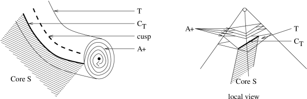
Figure 1: Spun normal surface

Definition 1.1.

Suppose that $M$ is the interior of a compact manifold with tori or Klein bottle boundary components and $\Gamma$ is an ideal triangulation of $M$. A spun normal surface $S$ has infinitely many normal disk types, of which finitely many are quadrilaterals and infinitely many are triangular. Moreover $S$ has a finite collection of boundary slopes, which are choices of closed curves ${C^{i}}_{T_{j}}$ as above, in the 1–skeleton of each boundary torus component $T_{j}$ of $M$, or in the orientable double cover $T_{j}$ of any Klein bottle component. We can glue together all except a finite number of the triangular disk types in $S$ to form a finite collection of half open spiralling annuli ${A^{ij}}_{+}$ or ${A^{ij}}_{-}$ as described above. Then the remaining finitely many quadrilateral and triangular disk types satisfy the compatibility equations, together with this finite collection of annuli which are viewed as having boundary curves given by the normal arc types of the curves ${C^{i}}_{T_{j}}$.

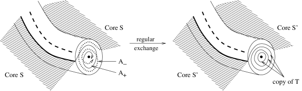
Figure 2: Extra or cancelling infinite half open annuli

Notice that we can have ‘extra’ or cancelling infinite half-open annuli at the same boundary component of $M$, since if a spun normal surface $S$ has copies of both $A_{+}$ and $A_{-}$ for a given boundary slope, then we can find a new spun normal surface or possibly just a normal surface $S^{\prime}$, by removing (or cancelling) these two annuli from $S$. Moreover $S$ might be embedded, immersed or have branch points. In the fifth paper of our sequence, it will be natural to consider also higher genus boundary surfaces for $M$. In that case, we must consider generally immersed spiralling annuli $A_{+},A_{-}$, as occur in the case of Klein bottle boundary components. These arise naturally, by projecting embedded annuli in a suitable covering space of a boundary surface $S$, to $M$.

It will be very convenient to extend our ideas of normal and spun normal surfaces, to allow negative numbers of triangular and quadrilateral disk types. For normal surfaces, this is easy; we just take all integer solutions of the compatibility equations and call these formal normal surfaces, to allow coordinates (multiples of the disk types) to be any integers, not just non-negative ones. For spun normal surfaces we can play the same game by allowing the half open annuli to occur with negative multiplicity as well as the disk types and have formal solutions of the compatibility equations as well. We will refer to these as formal spun normal surfaces.

Now to form a vector space $\mathcal{W}$ of formal spun and ordinary normal surfaces $S$, we will consider only the quadrilateral coordinates of each $S$. So $\mathcal{W}$ will be a subspace of $\mathbb{R}^{3k}$. This idea has been studied previously in [19], in case of ordinary normal surface theory in standard triangulations and is called $Q$–normal surface theory. For spun normal surfaces, $Q$–theory has been investigated in [10],[11]. There are $k$ compatibility equations for the quadrilaterals and we discuss this in detail later on. In an ideal triangulation, the solutions to these equations are naturally either normal or spun normal surfaces. The only surfaces which are not ‘seen’ by this theory, are multiples of the boundary Klein bottles and tori, formed entirely of triangular disk types. If we added these in also, the theory would have dimension $2k+2c$. However these boundary surfaces play no important role, so it is reasonable to leave them out of consideration. Spun normal surface theory has been used in an interesting way by Stefan Tillmann [18], to study essential splitting surfaces arising from representation varieties in Culler–Shalen theory.

In our fifth paper, we will prove an extension of an unpublished result of Thurston, namely that any immersed essential surface is homotopic to a spun normal surface, unless the surface lifts to a fibre of a bundle structure in some finite sheeted covering space. Consequently, if a certain boundary slope is not in the image of the boundary map (as in the examples in section 5 below) then either there are no immersed essential surfaces with such a boundary slope (in the homological sense of our boundary map), or any such a surface must be a virtual fibre.

Note that for the examples of the figure–8 knot complement and the Gieseking manifold in this paper, we are not able to get any interesting information on the boundary slopes of their immersed incompressible surfaces. These two examples are instances of layered triangulations of bundles, and the latter give special problems for the question of homotoping immersed incompressible surfaces to be spun normal. Full details are in the fifth paper.

2 The canonical basis for normal surface theory

In this section, we will construct a very useful ‘canonical basis’ for the solution space $\mathcal{V}$ of the compatibility equations for formal normal surface theory. This is independent of the details of the triangulation and the 3–manifold and was inspired by ideas of Casson, although he never stated a result like this. The theorem plays a key role in the second paper in our sequence, where we study the problem of deforming taut structures on ideal triangulations to angle structures.

Theorem 2.1.

Let $M$ be a 3–manifold with a triangulation $\Gamma$ which is either ideal or not, depending on whether $M$ is the interior of a compact manifold $N$ with tori and Klein bottle boundary components, or $M$ is closed. Assume there are $k$ tetrahedra and $e$ edges in $\Gamma$. Then $\mathcal{V}$ has a basis consisting of $k$ formal ‘tetrahedral’ surfaces and $e$ formal ‘edge’ surfaces.

Proof.

The idea is to study $e$ linear functionals $\phi_{1},\phi_{2},...,\phi_{e}$ from $\mathbb{R}^{7k}$ to $\mathbb{R}$, one for each edge $E_{1},E_{2},...,E_{e}$ of $\Gamma$. Each of these functionals restricts to $\mathcal{V}$ and we obtain $e$ linearly-independent functionals, which will be denoted by the same symbols. It then follows that $\mathcal{V}$ splits as a direct sum $\mathcal{A}\oplus\mathcal{B}$, where $\mathcal{A}$ is the common kernel of all the linear functionals and $\mathcal{B}$ is a ‘natural’ cokernel. We will then find bases of $\mathcal{A},\mathcal{B}$ separately and these will form our canonical basis.

For an edge $E_{i}$, let $d_{i}$ denote its degree, ie the number of copies of edges of tetrahedra which are glued together to form $E_{i}$. For every normal triangle or quadrilateral with $n$ vertices on $E_{i}$, we map this normal disk type to $\frac{n}{d_{i}}$. Extending by linearity gives a linear functional $\phi_{i}$ from $\mathbb{R}^{7k}$ to $\mathbb{R}$. To show these linear functionals restricted to $\mathcal{V}$ are linearly independent, we construct a collection of vectors $\beta_{1},\beta_{2},...,\beta_{e}$ in $\mathcal{V}$, so that $\phi_{i}(\beta_{j})=-2\delta_{ij}$, where as usual $\delta_{ij}=0$ if $i\neq j$ and $\delta_{ii}=1$. This will also show that $\beta_{1},\beta_{2},...,\beta_{e}$ is a basis for $\mathcal{B}$ as required. We call these vectors ‘edge’ solutions.

Consider the collection of triangular disk types which have at least one vertex on an edge $E_{i}$. We take $-n$ copies of each such a triangular disk, where the disk has precisely $n$ vertices on $E_{i}$, for $1\leq n\leq 3$. Similarly consider the set of tetrahedra which contain at least one edge which becomes $E_{i}$ after the faces and edges are glued together. Suppose $ABCD$ represents such a tetrahedron before gluing and $AB$ is an edge which becomes $E_{i}$. Then one copy of the quadrilateral separating $AB$ from $CD$ is selected. Notice that if the edge $CD$ also becomes $E_{i}$, then we must choose two copies of this quadrilateral. Do this for the $d_{i}$ edges of tetrahedra which are glued together to form $E_{i}$. Then $\beta_{i}$ is defined as this collection of negative triangular disks and positive quadrilateral disks.

We need to check that $\beta_{i}$ is indeed in $\mathcal{V}$, ie is a solution of the compatibility equations. This is straightforward – consider a face $ABC$ of a tetrahedron $ABCD$, where $AB$ is identified with $E_{i}$. For the normal arc type running between $AC$ and $AD$, there is a triangular disk (cutting off $A$) and a quadrilateral disk (separating $AB$ and $CD$) which are ‘glued’ along this arc. Notice the triangular disk is taken with sign $-1$ whereas the quadrilateral is taken with a positive sign. Hence the boundary arc types cancel out as required by the compatibility equations. Assume next that the tetrahedron $A^{\prime}B^{\prime}C^{\prime}D^{\prime}$ is glued to $ABCD$ by identifying $ABC$ with $A^{\prime}B^{\prime}C^{\prime}$. For the normal arc type running between $AB$ and $AC$, the triangular disk type cutting off $A^{\prime}$ is glued to the triangular disk cutting off $A$, along this arc. Since both disks have sign $-1$, the boundary arcs cancel. Finally, a similar argument applies for the normal arc type running between $AC$ and $BC$ by gluing two quadrilateral disk types, separating $AB$ and $CD$ (respectively $A^{\prime}B^{\prime}$ and $C^{\prime}D^{\prime}$) in the two tetrahedra. One can check that self-identification of tetrahedra does not affect this cancellation and so $\beta_{i}$ is a ‘formal’ normal surface, ie a solution of the compatibility equations. If there are no tetrahedra with two or more edges identified to $E_{i}$, the surface $\beta_{i}$ can be visualized as a cylindrical box with negative top and bottom and positive sides.

Next we observe that $\phi_{i}(\beta_{j})=-2\delta_{ij}$. It is clear that $\phi_{i}(\beta_{i})=-2$. If there are no tetrahedra with two or more edges identified to $E_{i}$, then the functional $\phi_{i}$ takes values $-1$ at the top and bottom ends of the box and $0$ at all other vertices. So the total value of $\phi_{i}(\beta_{i})$ is $-2$ as claimed. Again one can check that self-identifications do not affect this calculation. It remains to show that $\phi_{j}(\beta_{i})=0$ if $i\neq j$. (We have interchanged $i,j$ to use our previous description of the solution $\beta_{i}$). With notation as in the previous paragraph, assume that the edge $E_{j}$ is $AC$. Now there are two triangular disks with signs $-1$ and two quadrilateral disks with signs $+1$ coming from $\beta_{i}$, at this edge, so their contributions to $\phi_{j}(\beta_{i})$ cancel out. Self-identifications will not alter this phenomenon and so we have proved both that the surfaces $\beta_{1},\beta_{2},...,\beta_{e}$ are linearly independent and also that they form a basis for a cokernel $\mathcal{B}$ for the linear functionals $\phi_{1},\phi_{2},...,\phi_{e}$ on $\mathcal{V}$.

To complete the proof of this theorem, we need to construct a basis $\alpha_{1},\alpha_{2},...,\alpha_{t}$ for the kernel $\mathcal{A}$ of the linear functionals. Again let $ABCD$ denote the $i$th tetrahedron. Then $\alpha_{i}$ will be each of the $4$ triangular disk types cutting off a vertex taken with sign $-1$ and each of the $3$ quadrilateral disk types with sign $+1$ in this tetrahedron. We must check that $\alpha_{i}$ is in $\mathcal{V}$, ie solves the compatibility equations. This is very similar to the previous argument - for a normal arc type between edges $AB$ and $AC$, the triangular disk cutting off $A$ has sign $-1$ and the quadrilateral disk separating $AB$ and $CD$ has sign $+1$, so the two boundary arcs coming from these disks cancel as required.

It is equally easy to see that all the surfaces $\alpha_{1},\alpha_{2},...,\alpha_{t}$ are in the common kernel $\mathcal{A}$ of the linear functionals and that they are linearly independent, since they have no non-zero coordinates in common. The final step is to prove that these surfaces span $\mathcal{A}$. So we need to consider any vector $S$ which is in $\mathcal{A}$ and show it is a linear combination of $\alpha_{1},\alpha_{2},...,\alpha_{t}$. Notice that the ‘intersection number’ of $S$ with every edge is zero, since $S$ is in $\mathcal{A}$. If as usual, $ABCD$ is the $i$th tetrahedron of $\Gamma$, then the compatibility equations into a neighboring tetrahedron $A^{\prime}B^{\prime}C^{\prime}D^{\prime}$, where the face $ABC$ is glued to $A^{\prime}B^{\prime}C^{\prime}$, show that the total number $N$ (which can be positive or negative) of triangle and quadrilateral disks in $ABCD$ which meet $AB$ is the same as the total number of triangle and quadrilateral disks in $A^{\prime}B^{\prime}C^{\prime}D^{\prime}$ which meet $A^{\prime}B^{\prime}$. Following the tetrahedra around the edge $E_{i}$, which is $AB$ and $A^{\prime}B^{\prime}$ after identifications, we see this number $N$ is independent of the tetrahedron containing an edge identified to $E_{i}$. Since the value of the functional $\phi_{i}$ is exactly $Nd_{i}$, where $d_{i}$ is the degree of $E_{i}$, it follows that $N=0$, since $S$ is in $\mathcal{A}$. It is an easy exercise to check that the only sets of numbers of triangles and quadrilaterals in $ABCD$ which satisfy this condition for each of the $6$ edges of the tetrahedron, are multiples of $\alpha_{i}$. Hence this proves that $\alpha_{1},\alpha_{2},...,\alpha_{t}$ span $\mathcal{A}$ and the construction of the canonical basis is complete. ∎

RemarksFor ideal triangulations, where the 3–manifold $M$ is the interior of a compact 3–manifold with tori and Klein bottle boundaries, a simple Euler characteristic argument, using Poincaré duality, shows that $k=e$, ie the number of tetrahedra is equal to the number of edges. This is the case of most interest to us. Another important case is a triangulation of a closed 3–manifold with a single vertex [9]. Again a simple Euler characteristic argument shows then that $e=k+1$. So we conclude that the dimension of $\mathcal{V}$ is either $2k$ or $2k+1$ respectively in these two standard cases.

3 Dimension of spun and ordinary normal surface theory

In this section, we will give a lower bound on the dimension of formal spun normal surface theory, working with an ideal triangulation of $M$. We begin with a quick summary of $Q$–normal surface theory ([19], [10], [11]). Let $m_{1},m_{2},...,m_{3k}$ denote the number of quadrilateral normal disk types in an ordinary or spun normal surface. It is not hard to show that once the quadrilateral disks are specified, a formal normal or spun normal surface can be reconstituted, up to multiples of the boundary Klein bottles and tori. The key fact we need is that the quadrilaterals satisfy $k=e$ compatibility equations, one for each edge of $\Gamma$. These equations are readily found by eliminating the triangular coordinates from the ordinary compatibility equations in the previous section. Before introducing these equations, we note an important way of labelling the corners of the quadrilateral disk types, assuming that $M$ is orientable.

Let $ABCD$ and $A^{\prime}B^{\prime}C^{\prime}D^{\prime}$ be tetrahedra which are glued along the faces $ABC$ and $A^{\prime}B^{\prime}C^{\prime}$. Let $AB$ and $A^{\prime}B^{\prime}$ be identified with the $i$th edge $E_{i}$ of $\Gamma$. For the quadrilateral separating $AC$ and $BD$, we will associate corner signs, $+$ to the corners on $AB,CD$ and $-$ to corners on $AD,BC$ (see Figure 3). Similarly for the quadrilateral separating $AD$ and $BC$, $+$ is given to the corners on $AC,BD$ and $-$ to corners on $AB,CD$. In the adjacent tetrahedron $A^{\prime}B^{\prime}C^{\prime}D^{\prime}$, the signs are reversed. So for the quadrilateral separating $A^{\prime}C^{\prime}$ and $B^{\prime}D^{\prime}$ (respectively $A^{\prime}D^{\prime}$ and $B^{\prime}C^{\prime}$), we will associate corner signs, $-$ to the corners on $A^{\prime}B^{\prime},C^{\prime}D^{\prime}$ (respectively $A^{\prime}C^{\prime},B^{\prime}D^{\prime}$) and $+$ to corners on $A^{\prime}D^{\prime},B^{\prime}C^{\prime}$ (respectively $A^{\prime}C^{\prime},B^{\prime}D^{\prime}$) (see Figure 3). To show that this assignment of signs is consistent for all quadrilaterals simultaneously, we note that it is equivalent to introducing an orientation on each tetrahedron. For example, a right handed rule on the tetrahedron $ABCD$ can be viewed as having orientations from $A$ to $B$ on the edge $AB$ and then circulating from the face $ABD$ to the face $ABC$ so that the normal arc running between $AB$ and $AD$ cutting off $A$ is transformed into the normal arc running between $AB$ and $BC$ cutting off $B$ in the quadrilateral separating $AC$ and $BD$ (see Figure 3).

$A$$B$$C$$D$$A^{\prime}$$B^{\prime}$$C^{\prime}$$D^{\prime}$$E_{i}$$E_{i}$$+$$+$$+$$+$$-$$-$$-$$-$

Figure 3: Labelling the corners of quadrilateral disk types

We associate this with the positive sign in the corner of the quadrilateral at the corner on $AB$. It is easy to see that if the orientation of $AB$ is reversed, we still have a positive sign at this corner coming from the right hand rule. By translating a right handed system throughout $M$, we see that the consistency of signs is guaranteed. Now for an orientable manifold, we can define a quadrilateral compatibility equation by taking the sum of all quadrilateral types meeting a fixed edge $E_{i}$ with sign given by the corner of each quadrilateral at $E_{i}$. So half the quadrilaterals have sign $+$ and half have sign $-$.

On the other hand if $M$ is non-orientable, then choosing an orientation reversing loop passing through centers of tetrahedra and faces, following around the quadrilaterals in these tetrahedra will give an inconsistency in this choice of corner signs. However we can still give a sign to corners of quadrilaterals around each fixed edge $E_{i}$, but cannot do this consistently for all edges and corners simultaneously. We do obtain a similar compatibility equation in the non-orientable case, since it does not matter how the quadrilateral corner signs vary from one edge to the other.

We are now ready to give the main result of this section.

Theorem 3.1.

Let $M$ be the interior of a compact manifold with boundary components which are tori or Klein bottles. Let $\Gamma$ denote an ideal triangulation of $M$ and let $\mathcal{W}$ be the vector subspace of formal normal and spun normal surfaces. Then the dimension of $\mathcal{W}$ is at least $2k+c$, where $k$ is the number of edges in $\Gamma$ and $c$ is the number of boundary components.

Proof.

We first show that there is at least one redundancy in the set of $Q$–matching equations, if $M$ is orientable. For adding all the equations, each quadrilateral appears in at most 4 equations with a total of exactly two $+$ signs and two $-$ signs. Consequently the entries corresponding to this quadrilateral will cancel, ie the sum of all $Q$–matching equations is zero. This proves that we need at most $k-1$ matching equations and the dimension of $\mathcal{W}$ is at least $2k+1$.

$V_{1}$$V_{1}$$V_{1}$$V_{1}$$V_{1}$$V_{1}$$V_{1}$$V_{1}$$V_{1}$$V_{1}$$V_{2}$$V_{2}$$V_{2}$$V_{2}$$V_{2}$$V_{2}$$\oplus$$\oplus$$\oplus$$\oplus$$\oplus$$\oplus$$+$$+$$\ominus$$\ominus$$\ominus$$\ominus$$-$$-$$-$$-$$\sum\varepsilon(V_{1}V_{1}){=}0$$\sum\varepsilon(V_{1}V_{1}){=}0$$\sum\varepsilon(V_{1}V_{1}){=}\sum\varepsilon(V_{2}V_{2})$$\sum\varepsilon(V_{2}V_{2}){=}0$

Figure 4: The cases of two ideal vertices

The next step is to analyze the case when there is more than one boundary torus, supposing that $M$ is orientable. So there are several ideal vertices, $V_{1},V_{2},...,V_{c}$. Now label any tetrahedron $ABCD$ by specifying which ideal vertices are identified with $A,B,C,D$. Let us consider first the case that there are only two ideal vertices $V_{1},V_{2}$ (see Figure 4). There are 5 cases, depending on how many of the vertices $A,B,C,D$ are labelled $V_{1}$. We prove that adding all the matching equations corresponding to edges with both ends labelled $V_{1}$ gives the same result as adding over all edges with both vertices at $V_{2}$. So there is a second redundancy in the matching equations and the dimension of $\mathcal{W}$ is at least $2k+2$. Note that if the number $n\neq 2$ of vertices in some tetrahedron which are labelled $V_{1}$, then adding the appearances of a quadrilateral type in this tetrahedron over all matching equations corresponding to edges with both ends at $V_{1}$ will give zero. This is because the signs at the corners of the quadrilateral at such edges always cancel. For the final case of two vertices labelled $V_{1}$ and two labelled $V_{2}$, we see that the number of appearances of a quadrilateral type in the two sums of matching equations is the same. Consequently this case is complete.

Generally, if there are ideal vertices, $V_{1},V_{2},...,V_{c}$, then we find (by the same argument) that the sum of the matching equations at edges labelled $V_{1}V_{1}$ is equal to the sum of the matching equations at all edges labelled $V_{i}V_{j}$ for $i,j>1$ and similarly for $V_{2}V_{2},...,V_{c}V_{c}$. Note that by connectivity of the one-skeleton of $\Gamma$, we have paths of edges between any two ideal vertices. This is easily seen to imply that there are at least $c-1$ such redundant matching equations and one redundancy that the sum of all $Q$–matching equations is zero. Hence the dimension of $\mathcal{W}$ is at least $2k+c$. In fact, one can consider a collection of variables labelled $x_{ij}$, one for each equation which is a sum of the compatibility or matching equations at all edges labelled $V_{i}V_{j}$. Then our relations found above can be written as $x_{mm}=\Sigma\{x_{ij}:i,j\neq m\}$ for $m=1,2,\ldots,c-1$ and $\Sigma x_{ij}=0$. Now it is easy to put this system of linear equations into row-echelon form and check that the rank is indeed $c$, proving that there are at least $c$ redundant compatibility equations.

Assume next that $M$ is non-orientable. Let $\widetilde{M}$ denote the orientable double cover of $M$ with $\widetilde{\Gamma}$ the lifted triangulation. There are pairs of edges interchanged by the covering involution $\sigma$. We are interested in vectors of quadrilaterals which are invariant under the induced action of $\sigma$, since any lifted normal or spun normal surface will lift to such a vector. So we introduce $3k$ new independent variables, by forming a copy of $\mathbb{R}^{3k}$ embedded in $\mathbb{R}^{6k}$, given by $\alpha\rightarrow(\alpha,\sigma(\alpha))$ for a vector $\alpha$ in $\mathbb{R}^{3k}$. Our matching equations can be thought of as being located around two edges $E,\sigma(E)$ simultaneously. This is achieved by using the new variables, which are integer multiples of pairs of quadrilateral disks $(D,\sigma(D))$. As $\sigma$ reverses orientation, it must reverse our choice of signs of corners of quadrilateral disks in $\widetilde{M}$. Hence corresponding quadrilateral coordinates in $\widetilde{M}$ under the induced action of $\sigma$ are negatives of each other, ie $n(D,\sigma(D))$ corresponds to the pair of coordinates $(n,-n)$ in $\widetilde{M}$.

The conclusion is that we do get a similar theory to the orientable case, starting with $k$ matching equations and finding $c$ redundancies, proving the dimension estimate is also valid in the non-orientable case. Note that $c$ is the number of Klein bottle and tori boundary components of $M$, since each Klein bottle lifts to a torus which is invariant under $\sigma$ and a torus lifts to a pair of tori interchanged by $\sigma$. So since invariant boundary components or pairs of switched components give rise to redundancies, this is the correct definition of $c$.

To illustrate this, consider the simple case that $M$ has a single boundary component which is a Klein bottle or torus. This lifts to a $\sigma$–invariant torus or a pair of tori interchanged by $\sigma$ in $\widetilde{M}$. We can label the ideal vertex or vertices by this torus or tori. The single relation amongst our new pairs of quadrilateral coordinates becomes just that the sum of all the matching equations is zero. If there were more boundary components, then an analogous argument to the previous one shows that there is at least one redundancy amongst the matching equations of the pairs of quadrilateral coordinates for each boundary component of $M$.

Next, if there are two boundary components of $M$, then we get two classes of ideal vertices of $\widetilde{M}$. Each class is either a single vertex which is fixed under the action of $\sigma$ or a pair of vertices interchanged by $\sigma$. As previously, it is easy to check with our new coordinates, that the sum of all the matching equations for edges with both ends in one vertex class gives the same result as the sum over all edges with both ends in the other class. The general case follows the same pattern as before. ∎

4 The boundary map for spun normal surface theory

To complete the computation of the dimension of $\mathcal{W}$, we need to prove it is also bounded above by $2k+c$. To do this, we will define a boundary map $\partial\co\mathcal{W}\rightarrow\mathbb{R}^{2c}$, where the range of $\partial$ is the direct sum of all the homology groups $H_{1}(T_{i},\mathbb{R})$, where the $T_{i}$ are the tori boundary components or the orientable double covers of the Klein bottle boundary components of $M$, for $1\leq i\leq c$. A key property of $\partial$ is that its kernel $A$ is precisely the quadrilateral vectors corresponding to all formal normal surfaces in $\mathcal{W}$. Hence we can compute readily the dimension of $A$ as $2k-c$, since the natural projection $\mathcal{V}\rightarrow\mathcal{W}$, which erases the triangular coordinates of a normal class, has kernel generated by the boundary tori and Klein bottles, so has dimension $c$. Since the dimension of $\mathcal{V}$ is $2k$, we will see that the subspace $A$ of standard normal classes in $\mathcal{W}$ has dimension $2k-c$. Consequently, the dimension of $\mathcal{W}$ is at most $2k-c+2c=2k+c$ and the computation of dimension will be complete. Moreover we obtain the important result that $\partial$ has image of dimension $2c$, so maps onto a subgroup of finite index, when using $\mathbb{Z}$ coordinates. We compute the image of $\partial$ for the figure–8 knot space and Gieseking manifolds in the final section.

Theorem 4.1.

Let $M$ be the interior of a compact manifold with boundary components which are tori or Klein bottles. Let $\Gamma$ denote an ideal triangulation of $M$ and let $\mathcal{W}$ be the vector subspace of formal normal and spun normal surfaces. Then the dimension of $\mathcal{W}$ is $2k+c$, where $k$ is the number of edges in $\Gamma$ and $c$ is the number of boundary components. Moreover the boundary map $\partial\co\mathcal{W}\rightarrow\mathbb{R}^{2c}$ is onto and hence when using $\mathbb{Z}$ coefficients, it follows that $\partial$ has image of finite index in the direct sum $\mathbb{Z}^{2c}$ of the homology groups $H_{1}(T_{i},\mathbb{Z})$, where the $T_{i}$ are the tori boundary components or the orientable double covers of the Klein bottle boundary components of $M$, for $1\leq i\leq c$.

Proof.

As in the previous section, we begin with the case that $M$ is orientable, so we can put signs on all corners of quadrilateral disks in a consistent manner. We will then proceed to put orientations on all boundary arcs of quadrilaterals. As previously, let $ABCD$ denote a tetrahedron and consider the quadrilateral separating edges $AC$ and $BD$. Assume that a $+$ sign is attributed to the vertex on the edge $AB$ as in the previous section. We now orient the boundary arc of this quadrilateral running between the vertices $u,u^{\prime}$ on $AB,AD$ respectively with an arrow from $u$ to $u^{\prime}$ (see Figure 5). If $v,v^{\prime}$ are the vertices on the edges $BC,CD$ respectively, then the boundary edges are oriented in the directions $v^{\prime}v,uv,v^{\prime}u^{\prime}$, ie from a vertex of $+$ sign to a vertex of $-$ sign. Notice that if we adopt the convention that a triangular face has the tetrahedron behind it, with a normal boundary arc having the vertex cut off above it and the positive corner is on the left and the negative on the right, then the orientation of the arc is from left to right. All $4$ arcs are now oriented the same way by this convention, as are all arcs of all quadrilaterals.

$A$$B$$C$$D$$u$$u^{\prime}$$v$$v^{\prime}$$+$$-$$+$$-$

Figure 5: Orientation of the boundary arcs of a quadrilateral

Next we want to glue together quadrilaterals at corner vertices and possibly along some boundary arcs. Imagine two ‘adjacent’ quadrilaterals with such a vertex in common at some edge of $\Gamma$, eg the corner $u$ at the edge $AB$ in the previous paragraph for the first quadrilateral, chosen so that there is a wedge of triangular disks at $u$ between these two quadrilaterals on a (possibly spun) normal surface $S$. There could be an empty wedge, if these two quadrilaterals are actually glued along an edge, eg the edge $uu^{\prime}$, rather than just glued at the corner vertex $u$. Now it is easy to see the sign of the corner of the second quadrilateral at $u$ must be $-$, ie the signs of the two adjacent quadrilaterals at such a vertex are always opposite. So we proceed to glue together quadrilaterals with vertices on the same edge of $\Gamma$ with opposite signs at these vertices.

Notice by the compatibility equations for quadrilaterals, eventually at $u$ we find an even number of quadrilaterals with alternating signs glued together in this fashion. Do this for all vertices of all quadrilaterals in any formal vector of quadrilaterals in $\mathcal{W}$. We call this the quadrilateral part of the surface and denote it by $S_{Q}$. There are finitely many ways of producing a quadrilateral part of a normal surface, which can then be filled in by triangular disks to form $S$. If the boundary curves of $S_{Q}$ are inessential on the boundary tori of $M$, then we can complete $S$ using disks and once-punctured tori, and obtain a closed normal surface. If these curves are essential, we get a spun normal surface. See [10], [11] for further details on this.

Now the key point is that since our choice of orientations of boundary arcs is independent of the gluings, and when two quadrilaterals are glued along such an arc, then the two orientations cancel, we see that the total homology class of the boundary curves of $S$ is independent of the choice of gluing of $S$. Therefore we have proved that there is a well-defined map $\partial\co\mathcal{W}\rightarrow\mathbb{R}^{2c}$ from a normal class in $\mathcal{W}$ to a boundary homology class in the first homology of the boundary tori. As there are assumed to be $c$ boundary tori, the image is in $\mathbb{R}^{2c}$ as claimed.

It is possible to have a situation where this boundary homology class is zero but the surface $S$ is spun normal, for example if there are two essential parallel curves $C,C^{\prime}$ in the boundary of a core of $S$ and the surface is spinning around a boundary torus in opposite directions from $C,C^{\prime}$. It is easy to see that this cannot happen for an embedded surface $S$, but in the general case of singular surfaces, such behaviour cannot be ruled out. However we can cut off the two infinite half-open annuli of triangular disks in $S$ and replace by a compact annulus of triangular disks joining up $C,C^{\prime}$ to form a normal surface, which is no longer spun. This illustrates the general fact that the kernel of $\partial$ consists of classes which can be represented by standard normal surfaces.

To prove this, if there are several curves $C_{1},...,C_{m}$ in the boundary of a core of $S$ and the sum of the homology classes of these curves is zero, then we can fill in the curves by a cycle consisting of triangles in the boundary tori of $M$. This may be a singular choice, since the curves might intersect. The cancelling of the signs corresponds to the normality of the resulting possibly singular closed surface.

In the non-orientable case, we proceed in a similar manner to the previous section. Let $\widetilde{M}$ be the orientable double covering with covering transformation $\sigma$ and lifted triangulation $\widetilde{\Gamma}$. Any spun normal surface lifts to a $\sigma$–invariant surface or a pair of such surfaces in $\widetilde{M}$. Now the boundary map $\widetilde{\partial}$ takes such a surface or pair of surfaces to a $\sigma$–invariant homology class in the boundary tori of $\widetilde{M}$. Hence we can project this to a corresponding class in the boundary tori and Klein bottles of $M$, and hence define the boundary map in $M$. For a pair of tori interchanged by $\sigma$ this is easy, since we have a pair of homology classes in the tori which are the two lifts of a single class in a boundary torus of $M$. For a single $\sigma$–invariant torus covering a Klein bottle, a $\sigma$–invariant homology class or pair of classes interchanged by $\sigma$, both project to a homology class in the Klein bottle. Notice that the boundary of a spun normal surface is always a 2–sided curve, since it is the end of a half open annulus with infinitely many triangles projecting to a torus or Klein bottle. So we can again use $\mathbb{R}$ coefficients for convenience, without losing any information.

The argument in the introduction of this section shows that this map is onto and so using $\mathbb{Z}$ coefficients, the corresponding map has an image of finite index in $\mathbb{Z}^{2c}$.

An elegant alternative approach was suggested by the referee. When considering all possible gluings of a surface from the normal disk types, it is necessary to observe that the resulting boundary of the surface is independent of the choice of gluing. However, one can consider the sum of the oriented boundary arcs of each quadrilateral as forming a 1–chain. Then the sum of these quadrilateral boundary arcs is the boundary of the sum of the quadrilaterals, viewed as a 2–chain, since a pair of oppositely oriented boundary arcs, coming from two quadrilaterals which may be glued along these arcs or may not, depending on the way the normal surface is formed from the disk types, will cancel out in this 1–chain. Hence the sum, which is a 1–cycle because of the matching equations and gluing rule, is independent of the choice of how the quadrilaterals are glued up. ∎

In the final section we examine $\partial$ with $\mathbb{Z}$ coefficients more closely, for the simplest interesting orientable and non-orientable examples.

5 The figure–8 knot complement and the Gieseking manifold

In the previous section, we defined the boundary map $\partial\co\mathcal{W}\rightarrow\mathbb{R}^{2c}$ and showed that it has rank $2c$. Here the figure–8 knot complement is presented as an example for which the boundary map is not onto, using $\mathbb{Z}$ coefficients. Also we describe the Gieseking manifold as a non-orientable example.

Figure 6 shows an ideal triangulation of the figure–8 knot complement described by Thurston [17]. It has two tetrahedra, two edges and one torus cusp. Following the argument in the previous section, the vector space $\mathcal{W}$ of spun and ordinary normal surfaces in the figure–8 knot complement has dimension 5. Define the boundary map $\partial\co\mathcal{W}\rightarrow\mathbb{R}^{2}$ described in section 4. We compute the total homology classes of some normal surfaces which imply that the boundary map is not onto. For each tetrahedron in Figure 6, we have three types of quadrilaterals denoted by $Q_{1}$, $Q_{2}$ and $Q_{3}$ in $T$ and $Q^{\prime}_{1}$, $Q^{\prime}_{2}$ and $Q^{\prime}_{3}$ in $T^{\prime}$ (see Figure 7). Using the right hand rule, we give signs of corners of the quadrilaterals as in Figure 7.

$A$$B$$C$$D$$A$$B$$C$$D$$T$$T^{\prime}$12345678

Figure 6: An ideal triangulation of the figure–8 knot complement

$A$$B$$C$$D$$-1$$-1$$+1$$+1$$A$$B$$C$$D$$-1$$-1$$+1$$+1$$A$$B$$C$$D$$-1$$-1$$+1$$+1$$A$$B$$C$$D$$-1$$-1$$+1$$+1$$A$$B$$C$$D$$-1$$-1$$+1$$+1$$A$$B$$C$$D$$-1$$-1$$+1$$+1$$Q_{1}$$Q_{2}$$Q_{3}$$Q^{\prime}_{1}$$Q^{\prime}_{2}$$Q^{\prime}_{3}$$T$$T$$T$$T$$T$$T^{\prime}$

Figure 7: All quadrilateral disk types

Let $x_{i}$ and $y_{i}$ denote the number of quadrilaterals of $Q_{i}$ and $Q^{\prime}_{i}$ types respectively, for $i=1,2,3$. The following is the system of $Q$–matching equations of the figure–8 knot complement [10], for the two edges of the triangulation. As in Section 3, the sum of these two equations is zero, ie one of the two equations is redundant.

$$\left\{\begin{array}[]{l}-2x_{1}+x_{2}+x_{3}-2y_{1}+y_{2}+y_{3}=0\\ 2x_{1}-x_{2}-x_{3}+2y_{1}-y_{2}-y_{3}=0.\end{array}\right.$$

There are twenty (possible) fundamental solutions of the system. Among those, the following six are all the different solutions up to symmetry.

$$\begin{array}[]{l}s_{1}=(1,0,0,0,0,2),\\ s_{2}=(1,2,0,0,0,0),\\ s_{3}=(1,1,1,0,0,0),\\ s_{4}=(1,1,0,0,1,0),\\ s_{5}=(1,1,0,0,0,1),\\ s_{6}=(1,0,0,0,1,1).\\ \end{array}$$

It is known that the figure–8 knot complement has the symmetry group isomorphic to the dihedral group

$$D_{4}=\langle f,h|f^{4}=h^{2}=1,h\circ f\circ h^{-1}=f^{-1}\rangle.$$

So all the other fundamental solutions can be obtained by isometries in $D_{4}$. We will show that all the normal surfaces corresponding to the above six solutions have boundary with an even number at the first component of the total homology class. This will imply that the normal surfaces corresponding to all the other fundamental solutions have also such boundary curves. Hence the boundary map has image with only even numbers at the first component, so is not onto. (Our convention will be that the meridian curve will have homology class $(1,0)$ and the longitude will correspond to $(0,1)$ for suitable orientations, as described below).

We label the vertices of the ideal tetrahedra of the figure–8 knot complement as shown in Figure 6. Then the symmetries $f$ and $h$ can be represented by the following permutations of the eight vertices;

$$f=(1234)(5876)\qua\text{and}\qua h=(15)(26)(37)(48)$$

12345678$T$$T^{\prime}$$A_{1}$$A_{2}$$A_{4}$$B_{2}$$B_{3}$$B_{4}$$C_{1}$$C_{2}$$C_{3}$$D_{1}$$D_{3}$$D_{4}$$S$$A_{5}$$A_{6}$$A_{8}$$B_{6}$$B_{7}$$B_{8}$$C_{5}$$C_{7}$$C_{8}$$D_{5}$$D_{6}$$D_{7}$

Figure 8: All arc types

Table 1 shows the transformations of arc types in Figure 8 by the symmetries $f$ and $h$. The letter label of each arc type is given by the label of the face containing the arc type with subscript label being the vertex cut off by the arc type.

$A_{1}$

$A_{2}$

$A_{4}$

$B_{2}$

$B_{3}$

$B_{4}$

$C_{1}$

$C_{2}$

$C_{3}$

$D_{1}$

$D_{3}$

$D_{4}$

$f$

$C_{2}$

$C_{3}$

$C_{1}$

$D_{3}$

$D_{4}$

$D_{1}$

$B_{2}$

$B_{3}$

$B_{4}$

$A_{2}$

$A_{4}$

$A_{1}$

$h$

$A_{5}$

$A_{6}$

$A_{8}$

$B_{6}$

$B_{7}$

$B_{8}$

$D_{5}$

$D_{6}$

$D_{7}$

$C_{5}$

$C_{7}$

$C_{8}$

$A_{5}$

$A_{6}$

$A_{8}$

$B_{6}$

$B_{7}$

$B_{8}$

$C_{5}$

$C_{7}$

$C_{8}$

$D_{5}$

$D_{6}$

$D_{7}$

$f$

$C_{8}$

$C_{5}$

$C_{7}$

$D_{5}$

$D_{6}$

$D_{7}$

$B_{8}$

$B_{6}$

$B_{7}$

$A_{8}$

$A_{5}$

$A_{6}$

$h$

$A_{1}$

$A_{2}$

$A_{4}$

$B_{2}$

$B_{3}$

$B_{4}$

$D_{1}$

$D_{3}$

$D_{4}$

$C_{1}$

$C_{2}$

$C_{3}$

Table 1: Transformations of arc types by $f$ and $h$

Let $S$ be the spanning once-punctured torus for the knot which has the boundary curve $A_{1}C_{2}B_{3}D_{4}$ as shown in Figure 9. We let, for convenience, $L=A_{1}C_{5}B_{3}D_{7}$ be the curve going (homotopically) around the longitude of the torus cusp once so that it has the homology class $(0,1)$ (see Figure 9). Notice that the orientation of the boundary arcs of each quadrilateral is given in section 4 so that the orientation of the boundary curves of a quadrilateral surface $S_{Q}$ is also fixed automatically. From the table, we can see that $L$ is transformed to the curve $C_{2}B_{8}D_{4}A_{6}$, which also goes (homotopically) around the longitude once, by the symmetry $f$. By the symmetry $h$, $L$ is transformed to $A_{5}D_{1}B_{7}C_{3}$, which traverses the longitude (homotopically) in the opposite direction to $L$. $M=A_{4}$ is a curve going (homotopically) around the meridian with homology class $(1,0)$ and it is transformed to $C_{1}$ by $f$, and to $A_{8}$ by $h$. Hence the homology class of the meridian is preserved by both symmetries, but we need to determine whether its orientation is preserved or reversed. To do this, consider the curve $D_{1}D_{4}C_{3}C_{1}$ which follows (homotopically) the longitude once in the negative orientation and the meridian 2 times in the negative orientation (see Figure 9), This curve is transformed to $A_{2}A_{1}B_{4}B_{3}$ by $f$ and to $C_{5}C_{8}D_{7}D_{6}$, by $h$. In the first case, we see that the image curve winds (homotopically) around the longitude once in the negative orientation and the meridian twice in the positive orientation, whereas in the second case the curve is taken to itself (homotopically) with opposite orientation. So we conclude that $f$ preserves the homology class of $L$ but reverses that of $M$, whereas $h$ reverses both classes. Hence both $C_{1}$ and $A_{8}$ traverse the meridian (homotopically) in the opposite direction to $A_{4}$ (see Figure 9) and have the homology class $(-1,0)$. Also since $C_{1}$ is transformed to $B_{2}$ by $f$, and to $D_{5}$ by $h$, the homology classes of $B_{2}$ and $D_{5}$ are $(1,0)$. It follows automatically that $B_{6}$ and $D_{3}$ have the homology class $(-1,0)$. All the other non-trivial curves are linear combinations of the meridian and longitude.

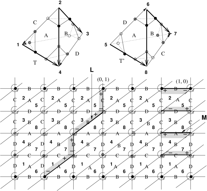
Figure 9: Boundary torus

Now we will compute the boundary curves of the spun and ordinary normal surfaces corresponding to the solutions $s_{1},s_{2},s_{3},s_{4},s_{5}$ and $s_{6}$. Since the total homology class of the boundary curves of any of the surfaces corresponding to a solution of the matching equations is independent of the choice of gluing, we choose our surfaces for convenience. Figure 9 is useful as a reference, when computing the boundary class. Notice that each of these solutions has Euler characteristic $-1$, since a quadrilateral has ‘negative curvature’ $-2\pi/3$, coming from its four vertices all lying on edges of degree $6$. Hence we expect each of the surfaces to be either a once-punctured Klein bottle, a twice-punctured projective plane or a thrice-punctured sphere, if all the boundary curves are essential. We can cap off any inessential boundary curves by disks in the torus at the cusp.

Let $F_{1}$ be a normal surface obtained from the solution $s_{1}$. The edges of the quadrilaterals of $F_{1}$ are $A_{1}$, $C_{2}$, $B_{3}$, $D_{4}$, $2B_{6}$, $2A_{8}$, $2C_{5}$ and $2D_{7}$. We may assume that the edges $C_{2}$ and $C_{5}$, and $D_{4}$ and $D_{7}$ are glued together and cancelled out in the boundary class. Hence the boundary of $F_{1}$ is the curve $A_{8}D_{7}A_{1}B_{6}B_{6}C_{5}B_{3}A_{8}$ which has the total homology class $(-4,1)$, ie winds once around the longitude and minus four times around the meridian (see Figure 10). Notice that as is well-known, at this slope, there is an embedded once-punctured Klein bottle, which is just the surface $F_{1}$.

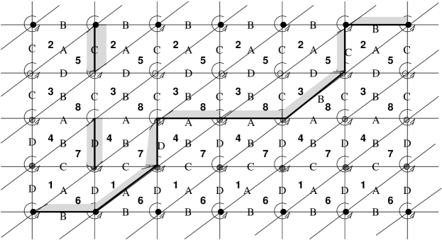
Figure 10: Boundary curves of $F_{1}$

Now for the solution $s_{2}=(1,2,0,0,0,0)$, a normal surface $F_{2}$ corresponding to $s_{2}$ has the following three boundary components; $A_{2}B_{3}B_{4}A_{1}$, $C_{1}C_{1}D_{4}B_{4}$, and $D_{3}D_{3}C_{2}A_{2}$ which have the homology classes $(-2,1)$, $(-1,0)$ and $(-1,0)$, respectively (see Figure 11). Hence the total homology class of the boundary curves of $F_{2}$ is $(-4,1)$. $F_{2}$ must be an immersed thrice-punctured sphere.

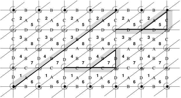
Figure 11: Boundary curves of $F_{2}$

Let $F_{3}$ be a normal surface corresponding to the solution $s_{3}$. We can choose the gluing so that $F_{3}$ has the boundary curves $A_{1}D_{1}B_{2}$, $B_{4}D_{4}C_{1}$, $B_{3}C_{3}A_{4}$ and $A_{2}C_{2}D_{3}$, all of which have the homology class (0,0) (see Figure 12). After capping off the trivial curves, this is a tetrahedral surface of the canonical basis defined in the section 2. Notice that the surface has branch points. Actually there is no gluing for an immersed normal surface corresponding to the solution $s_{3}$.

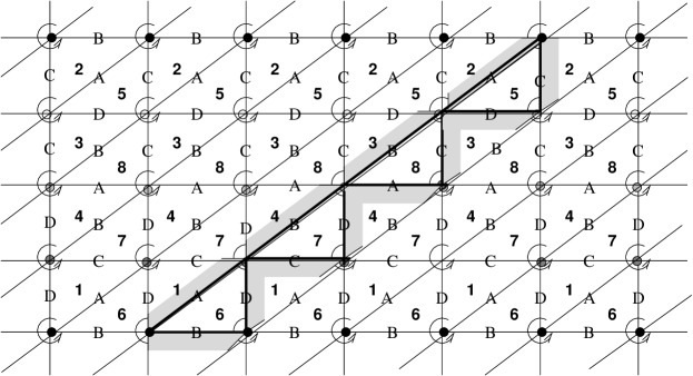
Figure 12: Boundary curves of $F_{3}$

Let $F_{4}$ be a normal surface corresponding to the solution $s_{4}=(1,1,0,0,1,0)$. We choose $F_{4}$ to have the boundary curves $B_{4}C_{1}D_{4}$ and $C_{2}A_{6}C_{7}A_{1}A_{2}$ which have the homology classes $(0,0)$ and $(2,0)$, respectively (see Figure 13). Hence the total homology class is $(2,0)$. As the case of $s_{3}$, there is no corresponding immersed normal surface to the solution $s_{4}$.

Figure 13: Boundary curves of $F_{4}$

For the solution $s_{5}=(1,1,0,0,0,1)$, a corresponding normal surface $F_{5}$ has the boundary curves $A_{2}B_{3}A_{8}D_{7}A_{1}$, $B_{4}D_{4}C_{1}$, $B_{6}$ and $D_{3}$. The homology classes of the curves are $(-2,1)$, $(0,0)$, $(-1,0)$ and $(-1,0)$ and the total homology class is $(-4,1)$ (see Figure 14). After capping off the trivial curve, this is an immersed thrice-punctured sphere.

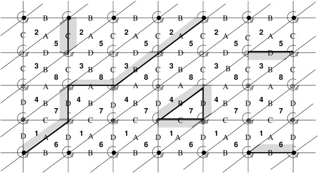
Figure 14: Boundary curves of $F_{5}$

Finally for the solution $s_{6}=(1,0,0,0,1,1)$, we can choose a normal surface $F_{6}$ which has boundary curves $A_{8}$, $B_{6}$, $C_{7}$ and $D_{5}$. Then the homology classes of the curves are $(-1,0)$, $(-1,0)$, $(1,0)$ and $(1,0)$, respectively and the total homology class of the boundary curves of $F_{6}$ is $(0,0)$ (see Figure 15). In this case, the surface has a branch point. Notice that there is no gluing for an immersed normal surface corresponding to the solution $s_{6}$.

Therefore all six solutions correspond to normal surfaces which have even numbers at the first component of the total homology class of the boundary curves. Since the normal surfaces corresponding to the other fundamental solutions are obtained from the normal surfaces corresponding to these six solutions by symmetries, and the symmetries transform the boundary curves as shown previously, the total homology classes of the boundary curves of any spun normal surfaces in the figure–8 knot complement have only even numbers at the first component. Hence the boundary map $\partial\co\mathcal{W}\rightarrow\mathbb{R}^{2}$ has image the subgroup of index $2$ consisting of all slopes of the form $(2m,n)$.

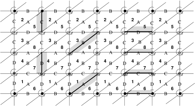
Figure 15: Boundary curves of $F_{6}$

Finally we study the Gieseking manifold, which has an ideal triangulation with one tetrahedron, one edge and a Klein bottle cusp. The Gieseking manifold is double-covered by the figure–8 knot complement and has covering transformation by the symmetry $f\circ h=(18)(25)(36)(47)$. Figure 16 shows the Gieseking manifold and a fixed orientation going around the unique edge.

1234$\widehat{1}$$\widehat{2}$$\widehat{3}$$\widehat{4}$$\widehat{5}$$\widehat{6}$$\widehat{1}$$\widehat{2}$$\widehat{3}$$\widehat{4}$$\widehat{5}$$\widehat{6}$$A$$A$$A$$A$$B$$B$$B$$B$$C$$C$$C$$C$$D$$D$$D$$D$

Figure 16: Gieseking manifold

$-1$$-1$$-1$$-1$$-1$$-1$$+1$$+1$$+1$$+1$$+1$$+1$$Q_{1}$$Q_{2}$$Q_{3}$$\widehat{AC}$$\widehat{AC}$$\widehat{AC}$$\widehat{DA}$$\widehat{DA}$$\widehat{CD}$$\widehat{DA}$$\widehat{CD}$$\widehat{CD}$$\widehat{BC}$$\widehat{BC}$$\widehat{BC}$$\widehat{DB}$$\widehat{DB}$$\widehat{DB}$$\widehat{AB}$$\widehat{AB}$$\widehat{AB}$

Figure 17: Signs of corners of quadrilaterals in the Gieseking manifold

We denote each wedge $\widehat{1},\widehat{2},\widehat{3},\widehat{4},\widehat{5}$ and $\widehat{6}$ by $\widehat{DA},\widehat{CD},\widehat{BC},\widehat{AC},\widehat{AB}$ and $\widehat{DB}$ according to the labels of the two adjacent faces and the fixed orientation going around the edge. Since the wedges $\widehat{CD},\widehat{AC}$ and $\widehat{DB}$ have the opposite orientations to the ones obtained by the right hand rule applied to each edge in the tetrahedron without identification (see the case of the figure–8 knot complement), the signs of corners of quadrilaterals are as shown in Figure 17. Therefore the $Q$–matching equation of the Gieseking manifold is

$$\begin{array}[]{l}-2x_{1}+x_{2}+x_{3}=0,\end{array}$$

where $x_{1}$, $x_{2}$ and $x_{3}$ are the number of quadrilaterals of type $Q_{1}$, $Q_{2}$ and $Q_{3}$, respectively. Then all positive solutions are generated by the following solutions

$$\begin{array}[]{l}t_{1}=(1,1,1),\\ t_{2}=(1,2,0),\\ t_{3}=(1,0,2).\\ \end{array}$$

Now we will compute the homology class of the boundary curves of normal surfaces corresponding to each solution $t_{1}$, $t_{2}$ and $t_{3}$. We will follow exactly the same procedure as in the case of the figure–8 knot complement.

Figure 18: Boundary Klein bottle of the Gieseking manifold

Figure 18 shows the Klein bottle cusp of the Gieseking manifold. Note that the orientation around each vertex along a column is shown in opposite directions alternately. This will assist in determining the signs of the homology classes of curves. Also we call the longitude the slope $L=A_{2}A_{1}B_{4}B_{3}$, which is equivalent to the curve $A_{1}D_{4}B_{3}C_{2}$, and the meridian the slope $M=B_{4}$ to conform to the figure–8 knot terminology (see Figure 18). Notice that $B_{4}$ lifts to $B_{4}D_{4}$, which is homotopic to the meridian slope $A_{4}$ of the torus cusp in the figure–8 knot complement, by the double covering map from the figure–8 knot complement onto the Gieseking manifold. Let the homology classes of $L$ and $M$ be $(0,1)$ and $(1,0)$, respectively. Then we get the homology classes of the following curves; $A_{2}\sim\overline{C_{2}}\sim D_{4}\sim\overline{B_{4}}$ with $(-1,0)$, $D_{3}\sim A_{4}\sim\bar{D_{4}}B_{4}$ with $(2,0)$, $A_{4}\sim\overline{C_{1}}\sim\overline{B_{2}}$ with $(2,0)$, $C_{3}B_{3}\sim C_{1}\sim B_{2}$ with $(-2,0)$ and $A_{1}D_{1}\sim A_{4}\sim D_{3}$ with $(2,0)$.

Let $G_{1}$ be a normal surface obtained from the solution $t_{1}=(1,1,1)$. We can choose $G_{1}$ to have boundary curves $D_{3}C_{3}B_{3}$, $A_{4}D_{4}B_{4}$, $C_{1}D_{1}A_{1}$ and $B_{2}C_{2}A_{2}$, all of which have the trivial homology class (see Figure 19). Hence the total homology class of the boundary curves of $G_{1}$ is $(0,0)$. Note that the curves, $D_{3}$, $A_{4}$, $C_{1}$, $B_{2}$, $C_{2}D_{1}D_{4}C_{3}$ and $A_{2}A_{1}B_{4}B_{3}$, are also the boundary curves of a normal surface obtained from the same solution but by another gluing. If we examine the orientations of the curves carefully, we will see that the curves have the homology class $(2,0)$, $(2,0)$, $(-2,0)$, $(-2,0)$, $(-4,-1)$ and $(4,1)$, respectively (see Figure 20). Hence the total homology class of these boundary curves is also trivial.

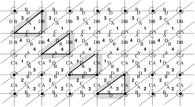
Figure 19: Boundary curves of $G_{1}$

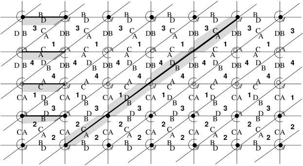
Figure 20: Boundary curves of another $G_{1}$

Next look at the solution $t_{2}=(1,0,2)$. We get a normal surface with boundary curves $C_{2}C_{3}A_{4}D_{4}D_{1}$, $B_{2}B_{2}$ and $A_{4}$ which have the homology classes $(2,-1)$, $(-4,0)$ and $(-2,0)$, respectively (see Figure 21). Then the total homology class is $(0,-1)$. Note that the edge pairs $D_{1}$ and $B_{3}$, and $C_{3}$ and $A_{1}$ cancel out.

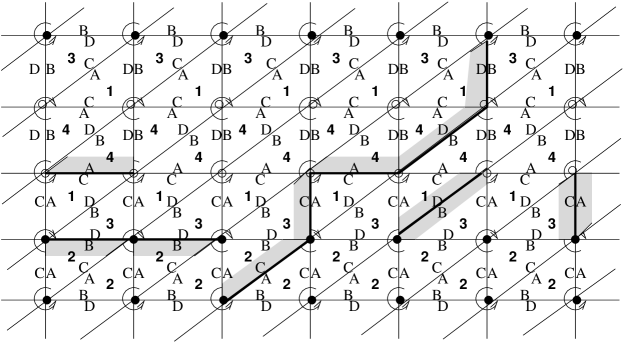
Figure 21: Boundary curves of $G_{2}$

Finally for the solution $t_{3}=(1,2,0)$, we get the following boundary curves: $D_{3}D_{3}A_{2}A_{1}B_{4}B_{3}$, $C_{2}A_{2}$ and $C_{1}C_{1}$ which have the homology class $(6,1)$, $(-2,0)$ and $(-4,0)$ (see Figure 22). The edge pair $D_{4}$ and $B_{4}$ cancels out. Hence the total homology class is $(0,1)$. Therefore as in the case of the figure–8 knot complement, the boundary map of the Gieseking manifold also has only multiples of 4 at the first component and is not onto. Note that for the first homology of the Klein bottle, the longitude is an element of order two. Hence we have found the image of the boundary map is a subgroup of index 4 of the group $\mathbb{Z}\oplus\mathbb{Z}_{2}$.

Figure 22: Boundary curves of $G_{3}$

Acknowledgements We would like to thank Stefan Tillmann for helpful conversations on spun normal surface theory and also an anonymous referee for a number of very helpful comments, which have improved the exposition. The second author is supported by a grant from the Australian Research Council.

Received:8 January 2004  Revised:29 March 2004

References

- [1] M Baker, On boundary slopes of immersed incompressible surfaces, Ann. Inst. Fourier (Grenoble) 46 (1996) 1443–1449 \MR1427132
- [2] M Baker, D Cooper, Immersed virtually-embedded boundary slopes, Top. Appl. 102 (2000) 239–252 \MR1745446
- [3] B Burton, E Kang, J H Rubinstein, Ideal triangulations of 3–manifolds III: Taut structures in low census manifolds, preprint (2002)
- [4] P Callahan, M Hildebrand, J Weeks, A census of cusped hyperbolic 3–manifolds, Math. of Comp. 68 (1999) 321–332 \MR1620219
- [5] D Coulson, O Goodman, C Hodgson, W Neumann, Computing arithmetic invariants of 3–manifolds, Experimental Math. 9 (2000) 127–152 \MR1758805
- [6] W Haken, Theorie der Normalflächen, Acta Math. 105 (1961) 245–375 \MR0141106
- [7] J Hempel, 3–manifolds, Annals of Math. Studies 86, Princeton University Press, Princeton, NJ (1976) \MR0415619
- [8] W Jaco, Lectures on three-manifold topology, CBMS Regional Conference Series in Mathematics 43. Amer. Math. Soc. Providence, R.I. (1980) \MR0565450
- [9] W Jaco, J H Rubinstein, 0–efficient triangulations of 3–manifolds, J. Differential Geom. 65 (2003) 61–168 \MR2057531
- [10] E Kang, Normal surfaces in knot complements, PhD thesis, University of Connecticut (1999)
- [11] E Kang, Normal surfaces in non-compact 3–manifolds, preprint (2001), to appear in J. Australian Math. Soc.
- [12] E Kang, J H Rubinstein, Ideal triangulations of 3–manifolds II: taut and angle structures, preprint (2002)
- [13] E Kang, J H Rubinstein, Ideal triangulations of 3–manifolds IV: immersed normal surface theory in angle structures, (in preparation)
- [14] E Kang, J H Rubinstein, Ideal triangulations of 3–manifolds V: existence of spun normal surfaces, (in preparation)
- [15] M Lackenby, Taut ideal triangulations of 3–manifolds, \gtref4200012369395 \MR1790190
- [16] E Moise, Affine structures in 3–manifolds V: the triangulation theorem and Hauptvermutung, Annals of Math. 55 (1952) 96–114 \MR0048805
- [17] W Thurston, The geometry and topology of 3–manifolds, lecture notes at Princeton University (1978)
- [18] S Tillmann, Degenerations and normal surface theory, PhD thesis, University of Melbourne (2002)
- [19] J Tollefson, Normal surface –theory, Pacific J. of Math. 183 (1998) 359–374 \MR1625962
Received:\qua8 January 2004 Revised:\qua29 March 2004