Abstract

It is conjectured by Pugh, Lins and de Melo in [7] that the system of equations

$$\begin{cases}\dot{x}=y-F(x)\\ \dot{y}=-x\end{cases}$$

has at most $n$ limit cycles when the degree of $F=2n+1$ or $2n+2$. Put $M$ for uniform upper bound of the number of limit cycles of all systems of equations of the form

$$\begin{cases}\dot{x}=y-(ax^{4}+bx^{3}+cx^{2}+dx)\\ \dot{y}=-x.\end{cases}$$

In this article, we show that $M\neq 2$. In fact, if an example with two limit cycle existed, one could give not only an example with $n+2$ limit cycles for the first system, but also one could give a counterexample to the conjecture $N(2,3)=2$ [see the conjecture $N(2,3)=2$ of F. Dumortier and C.Li, Quadratic Liénard equation with Quadratic Damping, J. Differential Equation, 139 (1997) 41 59]. We will also pose a question about complete integrability of Hamiltonian systems in ${\mathbb{R}}^{4}$ which naturally arise from planner Liénard equation. Finally, considering the Liénard equation as a complex differential equation, we suggest a related problem which is a particular case of conjecture. We also observe that the Liénard vector fields have often trivial centralizers among polynomial vector fields.

2000 AMS subject classification: 34C07.
Keywords: Limit cycles, Liénard equation.

1 Introduction

We consider Liénard equation in the form

$$\begin{cases}\dot{x}=y-F(x)\\ \dot{y}=-x\end{cases}$$ (1)

where $F(x)$ is a polynomial of degree $2n+1$ or $2n+2$. It is conjectured in [7] that this system has at most $n$ limit cycles. In particular, it was conjectured that the system

$$\begin{cases}\dot{x}=y-(ax^{4}+bx^{3}+cx^{2}+dx)\\ \dot{y}=-x\end{cases}$$ (2)

has at most one limit cycle. The phase portrait of (1) is presented in [7]. (1) has a center at the origin if and only if $F(x)$ is an even polynomial. The following useful Lemma is proved in [7]:

Lemma 1

Let $F(x)=E(x)+O(x)$ where $E$ is an even polynomial and $O$ is an odd polynomial, and that $O(x)=0$ has a unique root at $x=0$. Then system (1) does not have a closed orbit.

To prove the Lemma, it was shown that a first integral of the system

$$\begin{cases}\dot{x}=y-E(x)\\ \dot{y}=-x\end{cases}$$ (3)

that is analytic and defined on ${\mathbb{R}}^{2}-{0}$ is a monotone function along the solutions of (1). We introduce the following conjecture about the above first integral:

Conjecture 1

Let $E(x)$ be an even polynomial of degree at least 4, then there is no global analytic first integral for system (3) on ${\mathbb{R}}^{2}$.

The reason for conjecture: There are two candidates for defining a first integral, namely the square of the intersection of the solution with negative $y$ axis and the other the square of the intersection of the solution with $x$ axis. The first is well defined on ${\mathbb{R}}^{2}$ but certainly is not analytic at the origin and the second is analytic in the region of closed orbits but it can not be defined on all of ${\mathbb{R}}^{2}$. In fact, there are solutions not intersecting the $x$ axis: Consider the region surrounded by $y=\frac{-1}{x}$ and $y=0$ for $x\ggg 1$ and look at the direction field of

$$\begin{cases}\dot{x}=y-F(x)\\ \dot{y}=-x\end{cases}$$

on the boundary of this region. We conclude that there is a solution remaining in this area for all $t<0$ whenever the solution is defined. The analyticity of the second function, intersection with $x$ axis, is obtained by the fact that the 1 from $(y-E(x))dy+xdx$ is the pull back of $(y-g(x))dy+dx$ under $\pi(x,y)=(x^{2},y)$ with $E(x)=g(x^{2})$. Now, the differential equation

$$\begin{cases}\dot{x}=y-g(x)\\ \dot{y}=-1\end{cases}$$

does not have a singular point and the intersection of the orbits with $x$ axis defines an analytic function as a first integral, which we call $K(x,y)$. Then $K(x^{2},y)$ is a first integral for the original system (3). Note that putting $E(x)=x^{4}$, then the dual from of (3) is the pull back of Ricati equation, whose solution can not be determined in terms of elementary functions (This can be seen using Galois Theory, see [6]). I thank professor R. Roussarie for hinting me to this pull back. In line of the above conjecture, we propose the following question:

Question 1

Let an analytic vector field on the plane have a non degenerate center. As a rule, is it possible to define analytic first integrals globally in the domain of periodic solutions? (However, there is one locally.) In fact, using Riemann mapping theorem we can assume that the region of the center is all of ${\mathbb{R}}^{2}$.

We return to Liénard equation (1). The limit cycles of (1) correspond to fixed points of Poincaré return map. Let $F(x)$ has odd degree with positive leading coefficient. As a rule, we can not define Poincaré return map on positive $y$ semi axis. For example, if $F(x)=x^{2n+1}+2x$, in which case the singular point is a node, there is no solution starting on positive $y$ axis and returning again to this axis; see the direction field

$$\begin{cases}\dot{x}=y-(x^{2n+1}+2x)\\ \dot{y}=-x\end{cases}$$

on the semi line $y=x$ and $x>0$. Then, contrary to what is written in [7] or is pointed out in [10], we can define a Poincaré return map only in the case that origin is a weak or strong focus or in the case of existence of at least one limit cycle. In [10], it is also pointed out that Dulac’s problem is trivial for (1), that is, for any given $F(x)$, (1) has a finite number of limit cycles. Let $F(x)$ has odd degree, then $P_{0}=\lim_{y\rightarrow+\infty}P(y)$ exists and even we have $\lim_{y\rightarrow+\infty}(P(y)-P_{0})y^{i}=0$ for all $i$. Then $P$ has a finite number of fixed points. (In this work we do not use the strong approach $\lim_{y\rightarrow+\infty}y^{i}(P(y)-P_{0})=0$ and thus we do not prove it.) For the case that $F$ has even degree, the above is not trivial and one can deduce it from the results of this paper. In fact we must consider the case that $\lim_{y\rightarrow+\infty}P(y)=+\infty$. Equivalently, we have a loop at Poincaré sphere based at infinity. As a simple consequence of the above Lemma, we note that the system

$$\begin{cases}\dot{x}=y-x^{2}\\ \dot{y}=\epsilon(a-x)\end{cases}$$

does not has limit cycles for $a\neq 0$, because putting $x:=x+a$, $y:=y-a^{2}$ we will obtain

$$\begin{cases}\dot{x}=y-(x^{2}+2ax)\\ \dot{y}=-\epsilon x.\end{cases}$$

Using the Lemma, this system does not have a limit cycle. In figures on page 478 and 479 of [4], it appears that the existence of limit cycles is claimed.

2 Main Results

Theorem 1

For any $a,~{}b,~{}c$, there exists a unique $d=(a,b,c)$ such that the system (2) has a homoclinic loop in Poincaré sphere. This loop is stable if and only if the singular point is unstable.

Corollary 1

The maximum number of limit cycles of (2) can not be exactly two.

• (Proof of the theorem) For fixed $a,~{}b,~{}c,$ $a>0$, $b>0$, put $U(d)$ and $S(d)$ for intersection of unstable and stable manifolds corresponding to the topological saddle $(0,1,0)$ on the equator of Poincaré sphere. In fact $U(d)$ and $S(d)$ are similar to $P_{-}$ and $P_{+}$ on page 339 of [7], figure 3. $U(d)$ and $S(d)$ are continuous and monotone functions (as will be proved). We also prove $U(d)=S(d)$ has a unique root. First note that for $d>0$ there is no limit cycle or homoclinic loop based at infinity, using the lemma. Then we assume $d<0$, note that $U(0)>S(0)$, otherwise from the stability of the origin in (2) for $b>0$ and $d=0$, we would have a limit cycle for (2) which is a contradiction with the lemma. On the other hand, $U(d)\lll S(d)$ for $d\lll-1$ because the minimum value of $F(x)=ax^{4}+bx^{3}+cx^{2}+dx$ goes to $-\infty$ as $d\rightarrow-\infty$ and $S$ is decreasing. Now by continuity and monotonicity of $U$ and $S$ we have a unique root $d_{0}=\psi(a,b,c,)$ such that $U(d_{0})=S(d_{0})$. We must prove that $U$ and $S$ are continuous and monotone. It can be directly observed, even without using any classical theorem, that $U$, $S$ are continuous. We prove that $S$ is decreasing, similarly $U$ is increasing. Let $\gamma_{d}$ be a solution of $(2)_{d}$ that is asymptotic to the graph of $F(x)=ax^{4}+bx^{3}+cx^{2}+dx$, in $x<0$ in fact, $\gamma_{d}$ is the stable manifold for the topological saddle $(0,1,0)$ that intersects $y$ axis in $S(d)$. We prove that for $d^{\prime}<d<0$, $S(d^{\prime})>S(d)$. $\gamma_{d}$ is a curve without contact for $(2)_{d^{\prime}}$ and the direction field of $(2)_{d^{\prime}}$ on $\gamma_{d}$ is toward ”left” and the direction of $(2)_{d^{\prime}}$ on the semi line $y>0$. $x=0$, is toward ”right”. Then there is a unique orbit of $(2)_{d^{\prime}}$ that remains in the region surrounded by $\gamma_{d}$ and the semi line $x=0$, $y>0$. This orbit is a stable manifold for $(0,1,0)$ of system $(2)_{d^{\prime}}$, say; $\gamma_{d^{\prime}}$ certainly $\gamma^{\prime}_{d}$ can not intersect $\gamma_{d}$ so $\gamma_{d^{\prime}}$ will intersect negative $y$ axis in $S(d^{\prime})$ above $S(d)$. Therefore $S$ is decreasing. For the proof of the theorem it remains to prove that the loop is attractive, still assuming $a>0,~{}b>0,~{}d<0$. Before proving that the homoclinic loop is attractive we point out that, at first glance, this loop has a degenerate vertex at $(0,1,0)$, i.e. the linear part of vector field at the vertex is $\left[\begin{array}[]{cc}0&0\\ 0&0\\ \end{array}\right]$. But using weighted compactification as explained in [3], one has an elementary polycycle with two vertices, one vertex is a ”From” vertex and another is a “To”. Thus we do not have an “unbalanced polycycle” and therefore behavior of solution near the polycycle can not be easily determined. Thus, we use the following direct computation. (for definition of balanced and unbalanced polycycles, see [5] page 21.) Let $P_{0}=U(d_{0})=S(d_{0})<0$; We have a Poincaré return map $P$ defined on negative vertical section $(P_{0},0)$, we will prove that $\lim_{y\rightarrow P_{0}}P^{\prime}(y)=0$, then $P(y)-y$ is negative for $y$ near $P_{0}$. Note that considering the orbit of points near $P_{0}$ in the vertical section $(P_{0},0)$ is equivalent to considering the orbits of points $(0,\tilde{y})$ with $\tilde{y}\ggg 1$. Let $\gamma$ be the orbit of (2) corresponding to a homoclinic loop whose existence is proved above. $\gamma$ is asymptotic to the graph of $F(x)=ax^{4}+bx^{3}+cx^{2}+dx$.

  

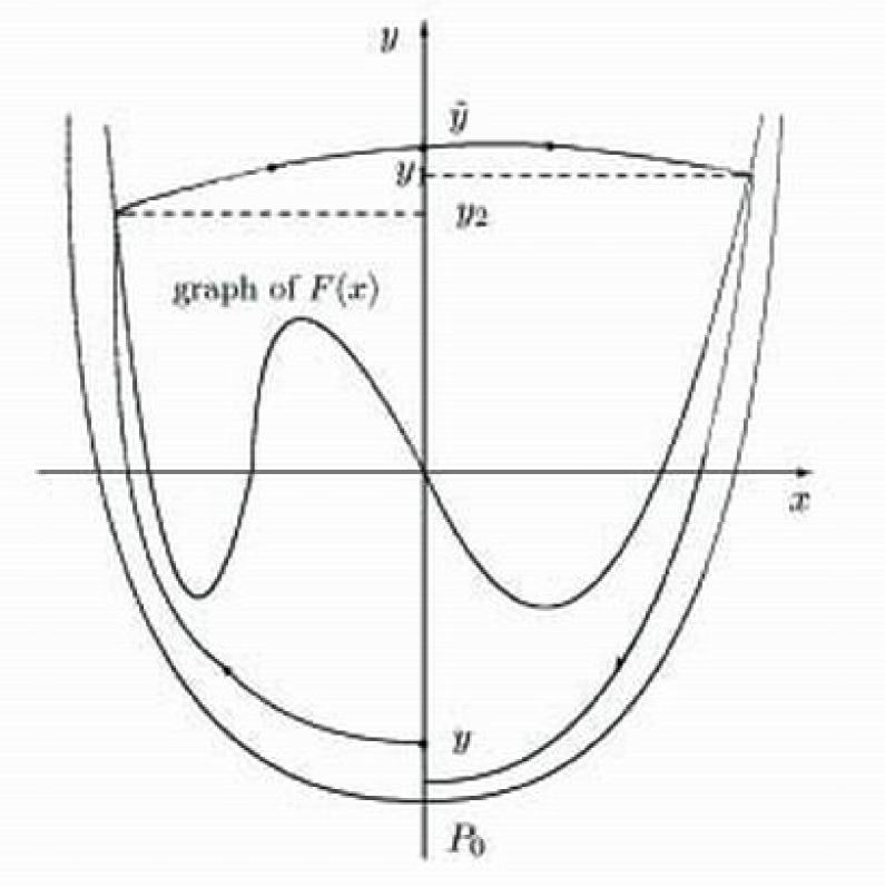
  Figure 1: $F(x)=ax^{4}+bx^{3}+cx^{2}+dx$

The orbit starting from $(0,\tilde{y})$ intersects the graph of $F$ at points with $y$ coordinates $y_{1}$ and $y_{2}$, when traced in positive and negative time direction, respectively. Recall that we want to prove $\lim_{y\rightarrow P_{0}}P^{\prime}(y)=0$; we use the following three facts:
I) There is a constant $K$ such that $|\tilde{y}-y_{1}|<K\sqrt{\tilde{y}}$ and $|\tilde{y}-y_{2}|<K\sqrt{\tilde{y}}$, where $K$ depends only on $a,b,c,d$.
II) $\gamma$ is asymptotic to the graph of $F$.
III) Let $A(y)$ and $B(y)$ two right inverse of $F(x)=ax^{4}+bx^{3}+cx^{2}+dx$, that is $F(A(y))=F(B(y))=y$ for $y\ggg 1$. Then $\lim_{y\rightarrow+\infty}(A(y)+B(y))=\frac{-b}{2a}$. (III) is a simple exercise (II) is pointed out in [7]: So we only prove the first. It suffices to prove (I), with the same notation $y_{1}$ and $y_{2}$ for the intersection of the orbit with the graph of $F(x)+1$ (in place of $F(x)$).$|\tilde{y}-y_{1}|=\frac{|\tilde{y}-y_{1}|}{\Delta x}\Delta x$, where $\Delta x$ is the $x$ coordinate of the intersection of the orbit starting from $(0,\tilde{y})$ with the graph of $F(x)+1$, then $\Delta x<K\sqrt{\tilde{y}}$ for some $K$, since the degree of $F$ is 4 and $\frac{\tilde{y}-y_{1}}{\Delta x}=\frac{-x}{y_{0}-f(x_{0})}$, where $(x_{0},y_{0})$ is a point of the trajectory starting at $(0,\tilde{y})$ and $0<x<\Delta x$ (using mean value theorem). Then $\frac{\tilde{y}-y_{1}}{\Delta x}<K\sqrt{\tilde{y}}$ and (I) is proved. Now we compute $\lim_{y\rightarrow P_{0}}P^{\prime}(y)$ (or equivalently for $\tilde{y}\ggg 1$ as stated above): $P^{\prime}(y)=\frac{y}{P(y)}exp[\int_{0}^{T(y)}``div^{\prime\prime}dt]$ where by “div” we mean the divergence of vector field (2). i.e. $-F^{\prime}(x(t))$, and $T(y)$ is the time of first return of the solution starting $(0,y)$ to negative vertical section (for the standard formula of $P^{\prime}(y)$ see [1]).

$$\int divdt=-\int F^{\prime}(x)dt=\int\frac{F^{\prime}(x)}{x}=\int\frac{-F^{\prime}(x)dr}{y-F(x)}$$

We use $\tilde{y}$ for the intersection of the solution starting at $(0,y)$ with the positive $y$ axis in positive time. We show that $\int_{0}^{T(y)}div=\int_{0}^{T(y)}-F^{\prime}(x(t))dt$ goes to $-\infty$ for $y$ near $P_{0}$. We divide $\int_{0}^{T(y)}divdt$ into three parts $I_{1}$, $I_{2}$, $I_{3}$: $I_{1}$ for the part of the integral that the orbit $\gamma_{y}$, the solution starting at $(0,y)$ for $y\in(p_{0},0)$ lice in $|x|<c$, where $c$ is a nonzero constant. $I_{2}$ corresponds to the part of $\gamma_{y}$ above the horizontal line $y=\tilde{y}-K\sqrt{\tilde{y}}$ where $K$ is the same constant which is given in (I), and $I_{3}$ is the remaining part of $I=\int_{0}^{T(y)}div$. In fact, in $I_{3}$ we compute the integral of the divergence of (2) along the part of $\gamma_{y}$ that lies below the horizontal line $y=\tilde{y}-K\sqrt{\tilde{y}}$ and outside of $|x|<c_{1}$ where in this part $\gamma_{y}$ lies between the graph of $F(x)$ and the orbit $\gamma$ which corresponds to the homoclinic loop. Note that as $\tilde{y}\rightarrow+\infty$ and consequently $y\rightarrow P_{0}$, $I_{2}$ and $I_{3}$ are very large in absolute value but $I_{1}$ remains bounded because $\int F^{\prime}(x)=\int\frac{F^{\prime}(x)dx}{y-F(x)}$. On the other hand we will see that $I_{2}+I_{3}$ goes to $-\infty$ as $y\rightarrow P_{0}$, thus we may ignore the term $I_{1}$. We could choose $K$ in (I) so that $|\frac{F^{\prime}(A(\tilde{y}))}{A(\tilde{y})}|<K\sqrt{\tilde{y}}$ where $A(\tilde{y})$ is the positive inverse of $F(x)$ for large $\tilde{y}$. There is a constant $K_{1}$ such that $|I_{2}|<K_{1}\tilde{y}$. Now we show $\frac{I_{3}}{\tilde{y}}$ to $-\infty$ as $y\rightarrow P_{0}$. Recall that $\tilde{y}$ is as in the figure. Applying III, we realize that $I_{3}$ is the integral of some function which is big in absolute value as $y\rightarrow P_{0}$ (or $\tilde{y}\rightarrow+\infty$). Generally speaking, let $g(\gamma)$ be a function such that $\lim_{y\rightarrow+\infty}g(\gamma)=+\infty$. Put $G(\gamma)=\int_{0}^{\gamma}g(s)ds$, then $\lim_{y\rightarrow+\infty}\frac{G(\gamma)}{\gamma}=+\infty$. So, it suffices to prove that $I_{3}$ is the integral of some function with respect to $\tilde{y}$, where this function goes to $-\infty$ as $\tilde{y}\rightarrow+\infty$.

$$I_{3}=\int\frac{F^{\prime}(x)}{x}dy,$$ (4)

$$\frac{F^{\prime}(x)}{x}=4ax^{2}+3bx+2c+dx.$$

We consider two parts of $\gamma_{y}$, one in $x>c$ and another in $x<-c_{1}$ since below the horizontal line $y=\tilde{y}-K\sqrt{\tilde{y}}$ the orbit $\gamma_{y}$ lies between $\gamma$ and graph of $F(x)$. Note that $\gamma$ is asymptotic to the graph of $F(x)$. Now, applying III, we will obtain $\frac{I_{3}}{y}\rightarrow-\infty$: for large values of $\tilde{y}_{1}$ the term $``\frac{d}{x}^{\prime\prime}$ in (1) can be omitted, then we must compute $-\lim_{\tilde{y}+\infty}4a(A^{2}(\tilde{y})-B^{2}(\tilde{y}))+3b(A(\tilde{y})-B(\tilde{y}))$, where $A(\tilde{y})$ and $B(\tilde{y})$ are inverses of $F(x)$ such that $F(A(\tilde{y}))=F(B(\tilde{y}))=\tilde{y}$ and $A(\tilde{y})>0$, $B(\tilde{y})<0$. We look at $-\lim_{\tilde{y}+\infty}(A(\tilde{y})-B(\tilde{y}))[4a(A(\tilde{y})-B(\tilde{y}))+3b]$. Certainly $(A(\tilde{y})-B(\tilde{y}))\rightarrow+\infty$. So, the above limit goes to $-\infty$ and $\frac{I_{3}}{\tilde{y}}\rightarrow+\infty$ as $y\rightarrow P_{0}$. This completes the proof of the theorem.

• (Proof of the corollary) From the proof of the theorem, we conclude that (2) can have an even number of limit cycles for $d\leq d_{0}=\psi(a,b,c)$ and can have odd number of limit cycles for $d_{0}<d<0$. Now let $(2)_{d}$ have exactly two limit cycles. therefore $d\leq d_{0}=\psi(a,b,c)$. If $d<d_{0}$, then $(2)_{d_{0}}$ has at least two limit cycles, counting multiplicity. It is because any closed orbit of $(2)_{d}$ is a curve without contact for $(2)_{d_{0}}$ and the direction fields of $(2)_{d_{0}}$ on this closed curve are toward the interior. But $(2)_{d_{0}}$ can not have an odd number of limit cycles. For instance let none of the two limit cycles of $(2)_{d_{0}}$ be semi stable. Then by a small perturbation $d=d_{0}-\epsilon$, (2); these two limit cycles do not die. On the other hand, we would obtain another limit cycle near the loop $\gamma$. Because for $d=d_{0}-\epsilon$, $\gamma$ is a curve without contact for $(2)_{d}$ and the direction of $(2)_{d}$ on $\gamma$ is toward the interior. Note that $\gamma$ was an attractive loop, therefore if $\epsilon$ is very small, using Poincaré Bendixson Theorem we will obtain a third limit cycle near the loop. Now any semi stable limit cycle can be replaced by two limit cycles by an appropriate perturbation $d=d_{0}\epsilon$ depending on which side of the limit cycle is stable. For instant, let $(2)_{d_{0}}$ have a semi stable limit cycle in interior of the loop then $d=d_{0}-\epsilon$ gives us two limit cycle near the semi stable ones and simultaneously one limit cycle near the loop. However the corollary is proved, we point out that the existence of 3 limit cycles for (2) easily implies the existence of 3 limit cycles for

  $$\begin{cases}\dot{x}=y-(ax^{4}+bx^{3}+cx^{2}+dx)\\ \dot{y}=-x+\epsilon x^{2}\end{cases}$$

  for small $\epsilon$. Now by a linear change of coordinates we put $\epsilon=1$, so we would obtain counterexample to the conjecture that the latter system for $\epsilon=1$ has at most 2 limit cycles. See conjecture $N(2,3)=2$ in [3].

Remark 1. For the proof of the existence of the loop $\gamma$ and also the proof of the corollary, in fact we used the rotational property of the parameter $d$ in (2), namely, any solution of $(2)_{d}$ is a curve without contact for $(2)_{d^{\prime}}$, if $d^{\prime}\neq d$. In particular, periodic solutions of $(2)_{d}$ are closed curves without contact for $(2)_{d^{\prime}}$. The simple but useful phenomenon of “rotated vector field theory” introduced by Duff, is some times used erroneously. See, for example , the investigation of

$$\begin{cases}\dot{x}=y-(ax^{4}+bx^{3}+dx)\\ \dot{y}=-x\end{cases}$$

in [8]. It is claimed that there is no limit cycle for $d<d_{0}=\psi(a,b,c)<0$, where $b>0$. In fact, the following situation that could occur, is not considered in [8]:
As we assumed above, let $a>0,~{}b>0$, for small $d<0$ we have exactly one (small) Hopf bifurcating limit cycle. It is possible that this limit cycle, before arriving to a loop situation, dies out in a semi stable limit cycle. Put $X={d|(5)_{d}{\rm hasexactlyonelimitcycle}}$, we do not necessarily have $d_{0}=infX$, where $d_{0}=\psi(a,b,0)$, correspond to loop situation. Put “i” for the above infimum. It could be $i>d_{0}$ and $(5)_{i}$ possesses a semi stable limit cycle. It is also possible that when the outermost limit cycle is dying out in the loop, the two innermost limit cycles have not arrived to each other yet. In fact [8] suggests an affirmative answer to the conjecture for system (2).

Remark 2. The homoclinic loop $\gamma$, as an orbit on the plane, not on the Poincaré sphere, divides the plane into two parts: its interior, where all solutions are complete, and its exterior, where all solutions have a finite interval of definition. Interior orbits are complete because $\gamma$ is a complete orbit by virtue of $\int dt=\int\frac{dx}{y-f(x)}$ and $\gamma$ being asymptotic to the graph of $F(x)$. The exterior points of $\gamma$ are not complete orbits because they tend to hyperbolic sink and the source on the equator of the Poincaré sphere (See [2]). Now, a trivial observation is that Liénard equation (1) can not have an isochronous center i.e. a center with a fixed period for all closed orbits surrounding it.

Remark 3. As we saw in the proof of the theorem and the corollary, the inequality $U(d)<S(d)$ or the reverse, determines oddness or evenness of the number of limit cycle. In this direction we point out that: Let $F(x)$ be an even degree polynomial with positive leading coefficient, and $U(\epsilon)$ and $S(\epsilon)$ be similar to $U(d)$ and $S(d)$ above for the system

$$\begin{cases}\dot{x}=y-F(x)\\ \dot{y}=-\epsilon x\end{cases}$$

Then $\lim_{\epsilon\rightarrow 0}U(\epsilon)=M^{+}$ and $\lim_{\epsilon\rightarrow 0}S(\epsilon)=M^{-}$ where $M^{-}$ and $M^{+}$ are minimum values of $F(x)$ on $(-\infty,0]$ and $[0,+\infty)$ resp. The proof is identical to the proof of existence of orbits passing through $U(d)$ and $S(d)$ asymptotic to the graph of $F(x)$, as in [7].

Remark 4. Note that when the degree of $F(x)$ in (1) is odd, the behavior of infinity is determined only by the sign of the leading term of $F(x)$. Then, giving an example of (2) with 3 limit cycles would give, inductively, $n+2$ limit cycles for (1), for all n.

Remark 5. Considering “flow” version of the problem of “centralizer of diffeomorphisms” described in [10] one can easily observe the following partial result. Let $L$ be the Liénard vector field similar to (1) with at least one closed orbit and $X$ be a polynomial vector field such that $[L,X]\equiv 0$, then $X=cL$ where $c$ is a constant real number. In general, let two vector fields have commuting flows and $\gamma$ be a closed orbit for one of them which does not lie in an isochronous band of closed orbits. Then $\gamma$ must be invariant by another vector field and if both vector fields are polynomials. Then either $\gamma$ is an algebraic curve or two vector fields are constant multiple of each other. But Liénard systems do not have algebraic solutions, [9]. More generally by the following proposition we have “Non existence of algebraic solution implies triviality of centralizer”.

Proposition 1

Let $M$ be the set of all polynomial vector fields on ${\mathbb{C}}^{2}$. Then $X\in M$ has trivial centralizer if $X$ dose not have an algebraic solution.

• Let $[X,Y]=0$. Then $X.Det(X,Y)=(DivX).(Det(X,Y))$, so $``Det(X,Y)=0^{\prime\prime}$ defines an algebraic curve invariant under $X$ (By $Det(X,Y)$) we mean the determinant of a 2 2 matrix whose columns are components of $X$ and $Y$).

Remark 6. The following could be a (real) generalization of formula used in proof of proposition:
Let $(M,\omega)$ be a $2n$ dimensional symplectic manifold and $X,Y$ two vector fields with the condition $[X,Y]\equiv 0$, then $X.\omega(X,Y)=n(DivX)\omega(X,Y)$. This formula is trivial for usual symplectic structure of ${\mathbb{R}}^{2}$. Further there is a local chart around each point of a two dimensional symplectic manifold that $\omega$ can be represented in the trivial form. Thus the formula is proved for arbitrary two dimensional symplectic manifold. Now, in general case we have a two dimensional symplectic submanifold $N$ of $M$, that $X$ and $Y$ are tangent to $N$. (For points $m\in M$ that $\omega(X(m),Y(m))\neq 0$, using Frobenius theorem.) From other hand $DivX_{M}=nDivX_{N}$. The investigation of points $m$ that $\omega(X(m),Y(m))=0$ is trivial. Then the proof is completed.

Question 2

Dirac introduced the following embedding of planner vector fields into Hamiltonian system in ${\mathbb{R}}^{4}:H=zP(x,y)+wQ(x,y)$. Now we consider the Hamiltonian $H=z(y-F(x))-wx$. When is this Hamiltonian completely integrable?

By completely integrable Hamiltonian, we mean that there is a first integral for the system

$$\begin{cases}\dot{x}=y-F(x)\\ \dot{y}=-x\\ \dot{z}=w-F^{\prime}(x)z\\ \dot{w}=-z\end{cases}$$

independent of $H$.
The particular case $F(x)=x^{2}$ for which (1) has a center with global first integral $\phi(x,y)=(y-x^{2}+\frac{1}{2})e^{-2y}$, suggests that when (1) does not have a center, the above Hamiltonian is not completely integrable. In fact, the function $\phi$, as above, is a first integral, independent of $H$ for above four dimensional system. Then, when (1) is not integrable, one expects that the corresponding Hamiltonian is not completely integrable. However, surprisingly, putting $F(x)=kx$, we have another first integral $yw+xz$.

Question 3

Considering (1) as a vector field on ${\mathbb{C}}^{2}$, and in line of conjecture in [7] one can think of the validity of the following two statement.
I)There are at most n different leaves containing real limit cycles.
II)There are at most n real limit cycles lying on the same leaf. By “leaf” we mean a leaf of the foliation corresponding to the equation (1) on ${\mathbb{C}}^{2}-{0}$.

Acknowledgement. The author thanks Professor S. Shahshahani for fruitful conversations. He also acknowledges the financial support of the Institute for Studies in Theoretical Physics and Mathematics.

References

- [1] A. A. Andronov et al, “Theory of Bifurcations of Dynamical System on the Plane”, Israel Program for Scientific Translation Jerusalem, 1971.
- [2] C. Chicone and J. Sotomayor, On a Class of Complete Polynomial Vector Fields in the Plane, J. Differential Equation 61 (1986), 398 418.
- [3] F. Dumortier and C. Li, Quadratic Li enard equation with Quadratic Damping, J. Differential Equation 139 (1997) 41 59.
- [4] W. Eckhause, Relaxation Oscillations Including a Standard Chase on French Ducks, In Asymptotic Analysis II, Springer Lecture Notes in Math. 985 (1983), 449 491.
- [5] Yu. S. IlYashenko “Finiteness Theorem of Limit Cycles”, Translation of Mathematical Monographs, Vol. 94, 1991.
- [6] I. Kaplansky, “An Introduction to Differential Algebra”, Herman Press, 1976.
- [7] A. Lins, W. demelo, C. C. Pugh, On Liénard Equation, Proc. Symp. Geom. and Topol. Springer Lecture Notes 597 (1977), 335 357.
- [8] Maoan. Han, Global Behavior of Limit Cycles in Rotated Vector Fields, J. Differential Equations 151 (1999), 20 35. 12
- [9] K. Odani, The limit Cycle of the Van der pol Equation is not Algebraic, J. Differential Equations 115 (1995), 146 152.
- [10] S. Smale, Mathematical Problems for Next Century, The Mathematical Intelligencer 20 (1998), 7 15.