Rigidity result for certain 3-dimensional singular spaces and their fundamental groups.

Abstract

In this paper, we introduce a particularly nice family of $CAT(-1)$ spaces, which we call hyperbolic P-manifolds. For $X^{3}$ a simple, thick hyperbolic P-manifold of dimension $3$, we show that certain subsets of the boundary at infinity of the universal cover of $X^{3}$ are characterized topologically. Straightforward consequences include a version of Mostow rigidity, as well as quasi-isometry rigidity for these spaces.

1 Introduction.

In this paper, we prove various rigidity results for certain 3-dimensional hyperbolic P-manifolds. These spaces form a family of stratified metric spaces built up from hyperbolic manifolds with boundary (a precise definition is given below). The main technical tool is an analysis of the boundary at infinity of the spaces we are interested in. We introduce the notion of a branching point in an arbitrary topological space, and show how branching points in the boundary at infinity can be used to determine both the various strata and how they are pieced together. The argument for this relies on a result which might be of independant interest: a version of the Jordan separation theorem that applies to maps $S^{1}\rightarrow S^{2}$ which are not necessarily injective. In this section, we introduce the objects we are interested in, provide some basic definitions, and state the theorems we obtain. The proof of the main theorem will be given in section 2. The various applications will be discussed in section 3. We will close the paper with a few concluding remarks and open questions in section 4.

Acknowledgments.

The results contained in this paper were part of the author’s thesis, completed at the University of Michigan, under the guidance of professor R. Spatzier. The author would like to thank his advisor for his help throughout the author’s graduate years. The author would also like to thank professor J. Heinonen for taking the time to proofread his thesis and to comment on the results contained therein. Finally, the author gratefully acknowledges the referee’s efforts in catching numerous minor errors in the first draft of this paper.

1.1 Hyperbolic P-manifolds.

Definition 1.1.

We define a closed $n$-dimensional piecewise manifold (henceforth abbreviated to P-manifold) to be a topological space which has a natural stratification into pieces which are manifolds. More precisely, we define a $1$-dimensional P-manifold to be a finite graph. An $n$-dimensional P-manifold ($n\geq 2$) is defined inductively as a closed pair $X_{n-1}\subset X_{n}$ satisfying the following conditions:

• Each connected component of $X_{n-1}$ is either an $(n-1)$-dimensional P-manifold, or an $(n-1)$-dimensional manifold.

• The closure of each connected component of $X_{n}-X_{n-1}$ is homeomorphic to a compact orientable $n$-manifold with boundary, and the homeomorphism takes the component of $X_{n}-X_{n-1}$ to the interior of the $n$-manifold; the closure of such a component will be called a chamber.

Denoting closure of the connected components of $X_{n}-X_{n-1}$ by $W_{i}$, we observe that we have a natural map $\rho:\coprod\partial W_{I}\longrightarrow X_{n-1}$ from the disjoint union of the boundary components of the chambers to the subspace $X_{n-1}$. We also require this map to be surjective, and a homeomorphism when restricted to each component. The P-manifold is said to be thick provided that each point in $X_{n-1}$ has at least three pre-images under $\rho$. We will henceforth use a superscript $X^{n}$ to refer to an $n$-dimensional P-manifold, and will reserve the use of subscripts $X_{n-1}\ldots X_{1}$ to refer to the lower dimensional strata. For a thick $n$-dimensional P-manifold, we will call the $X_{n-1}$ strata the branching locus of the P-manifold.

Intuitively, we can think of P-manifolds as being “built” by gluing manifolds with boundary together along lower dimensional pieces. Examples of P-manifolds include finite graphs and soap bubble clusters. Observe that compact manifolds can also be viewed as (non-thick) P-manifolds. Less trivial examples can be constructed more or less arbitrarily by finding families of manifolds with homeomorphic boundary and glueing them together along the boundary using arbitrary homeomorphisms. We now define the family of metrics we are interested in.

Definition 1.2.

A Riemannian metric on a 1-dimensional P-manifold (finite graph) is merely a length function on the edge set. A Riemannian metric on an $n$-dimensional P-manifold $X^{n}$ is obtained by first building a Riemannian metric on the $X_{n-1}$ subspace, then picking, for each chamber $W_{i}$ a Riemannian metric with totally geodesic boundary satisfying that the gluing map $\rho$ is an isometry. We say that a Riemannian metric on a P-manifold is hyperbolic if at each step, the metric on each $W_{i}$ is hyperbolic.

Figure 1: Example of a simple, thick P-manifold.

A hyperbolic P-manifold $X^{n}$ is automatically a locally $CAT(-1)$ space (see Chapter II.11 in Bridson-Haefliger [5]. Furthermore, the lower dimensional strata $X_{i}$ are all totally geodesic subspaces of $X^{n}$. In particular, the universal cover $\tilde{X}^{n}$ of a hyperbolic P-manifold $X^{n}$ is a $CAT(-1)$ space (so is automatically $\delta$-hyperbolic), and has a well-defined boundary at infinity $\partial^{\infty}\tilde{X}^{n}$. Finally we note that the fundamental group $\pi_{1}(X_{n})$ is a $\delta$-hyperbolic group.

We also note that examples of hyperbolic P-manifolds are easy to obtain. In dimension two, for instance, one can take multiple copies of a compact hyperbolic manifold with totally geodesic boundary, and identify the boundaries together. In higher dimension, one can similarly use the arithmetic constructions of hyperbolic manifolds (see Borel-Harish-Chandra [2]) to find hyperbolic manifolds with isometric totally geodesic boundaries. Gluing multiple copies of these together along their boundaries yield examples of hyperbolic P-manifolds. More complicated examples can be constructed by finding isometric codimension one totally geodesic submanifolds in distinct hyperbolic manifolds. Once again, cutting the manifolds along the totally geodesic submanifolds yield hyperbolic manifolds with totally geodesic boundary, which we can glue together to build hyperbolic P-manifolds (see the construction of non-arithmetic lattices by Gromov-Piatetski-Shapiro [9]).

Definition 1.3.

We say that an $n$-dimensional P-manifold $X^{n}$ is simple provided its codimension two strata is empty. In other words, the $(n-1)$-dimensional strata $X_{n-1}$ consists of a disjoint union of $(n-1)$-dimensional manifolds.

An illustration of a simple, thick P-manifold is given in figure 1. It has four chambers, and two connected components in the codimension one strata. We point out that P-manifolds show up naturally in the setting of branched coverings. Starting from a hyperbolic manifold $M$, one can take a totally geodesic codimension two subspace $N\subset M$, with the property that $N$ bounds a codimension one totally geodesic subspace $W$. One could look at a ramified cover $\bar{M}_{i}$ of $M$, of degree $i$, where the ramification is over $N$. This naturally inherits a (singular) CAT(-1) metric from the metric on $M$ (note that Gromov-Thurston [10] have shown that, when $i$ is sufficiently large, it is possible to smooth this singular metric to a negatively curved Riemannian metric). The pre-image $X\subset\bar{M}_{i}$ of the subspace $W\subset M$ will be a simple hyperbolic P-manifold, isometrically embedded in $\bar{M}_{i}$ (with respect to the singular metric). The codimension one strata in $X$ will consist of a single connected component, isometric to $N$, and there will be $i$ chambers, each isometric to $W$.

We also point out that related spaces include hyperbolic buildings. Indeed, these share the property that they are naturally stratified spaces, built out of pieces that are isometric to subsets of hyperbolic space. The difference lies in that for hyperbolic buildings, the boundary of the chambers are not totally geodesic in the space. Hyperbolic buildings have been studied by Bourdon-Pajot [4]; they obtain quasi-isometric rigidity for some 2-dimensional hyperbolic buildings (compare to our Theorem 1.3). Note that, unlike hyperbolic P-manifolds, hyperbolic buildings can only exist in low dimensions ($\leq 29$). This follows from a result of Vinberg [21], showing that compact Coxeter polyhedra do not exist in hyperbolic spaces of dimension $\geq 30$. Since the existence of such polyhedra is a pre-requisite for the existence of hyperbolic buildings, Vinberg’s result immediately implies the desired non-existence result.

Next we introduce a locally defined topological invariant. We use $\mathbb{D}^{n}$ to denote a closed $n$-dimensional disk, and $\mathbb{D}^{n}_{\circ}$ to denote its interior. We also use $\mathbb{I}$ to denote a closed interval, and $\mathbb{I}_{\circ}$ for its interior.

Definition 1.4.

Define the 1-tripod $T$ to be the topological space obtained by taking the join of a one point set with a three point set. Denote by $*$ the point in $T$ corresponding to the one point set. We define the $n$-tripod ($n\geq 2$) to be the space $T\times\mathbb{D}^{n-1}$, and call the subset $*\times\mathbb{D}^{n-1}$ the spine of the tripod $T\times\mathbb{D}^{n-1}$. The subset $*\times\mathbb{D}^{n-1}$ separates $T\times\mathbb{D}^{n-1}$ into three open sets, which we call the open leaves of the tripod. The union of an open leaf with the spine will be called a closed leaf of the spine. We say that a point $p$ in a topological space $X$ is $n$-branching provided there is a topological embedding $f:T\times\mathbb{D}^{n-1}\longrightarrow X$ such that $p\in f(*\times\mathbb{D}^{n-1}_{\circ})$.

It is clear that the property of being $n$-branching is invariant under homeomorphisms. We show some examples of branching in Figure 2. Note that, in a simple, thick P-manifold of dimension $n$, points in the codimension one strata are automatically $n$-branching. One can ask whether this property can be detected at the level of the boundary at infinity. This motivates the following:

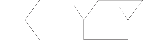
Figure 2: Examples of 1-branching and 2-branching.

Conjecture: Let $X^{n}$ be a simple, thick hyperbolic P-manifold of dimension $n$, and let $p$ be a point in the boundary at infinity of $\tilde{X}^{n}$. Then $p$ is $(n-1)$-branching if and only if $p=\gamma(\infty)$ for some geodesic ray $\gamma$ contained entirely in a connected lift of $X_{n-1}$.

One direction of the above conjecture is easy to prove (see Proposition 2.1). In the case where $n=3$, we will see that the reverse implication also holds. Note that in general, the (local) topological structure of the boundary at infinity of a $CAT(-1)$ space (or of a $\delta$-hyperbolic group) is very hard to analyze. The conjecture above says that with respect to branching, the boundary of a simple, thick hyperbolic P-manifold of dimension $n$ is particularly easy to understand.

In our proofs, we will make use of a family of nice metrics on the boundary at infinity of an arbitrary $n$-dimensional hyperbolic P-manifold (in fact, on the boundary at infinity of any CAT(-1) space).

Definition 1.5.

Given an $n$-dimensional hyperbolic P-manifold, and a basepoint $*$ in $\tilde{X}^{n}$, we can define a metric on the boundary at infinity by setting $d_{\infty}(p,q)=e^{-d(*,\gamma_{pq})}$, where $\gamma_{pq}$ is the unique geodesic joining the points $p,q$ (and $d$ denotes the distance inside $\tilde{X}_{n}$).

The fact that $d_{\infty}$ is a metric on the boundary at infinity of a proper $CAT(-1)$ space follows from Bourdon (Section 2.5 in [3]). Note that changing the basepoint from $*$ to $*^{\prime}$ changes the metric, but that for any $p,q\in\partial^{\infty}(X^{n})$, we have the inequalities:

$$A^{-1}\cdot d_{\infty,*}(p,q)\leq d_{\infty,*^{\prime}}(p,q)\leq A\cdot d_{\infty,*}(p,q)$$

where $A=e^{d(*,*^{\prime})}$, and the subscripts on the $d_{\infty}$ refers to the choice of basepoint used in defining the metric. In particular, different choices for the basepoint induce the same topology on $\partial^{\infty}\tilde{X}^{n}$, and this topology coincides with the standard topology on $\partial^{\infty}\tilde{X}^{n}$ (the quotient topology inherited from the compact-open topology in the definition of $\partial^{\infty}\tilde{X}^{n}$ as equivalence classes of geodesic rays in $\tilde{X}^{n}$). This gives us the freedom to select basepoints at our convenience when looking for topological properties of the boundary at infinity.

1.2 Statement of results, outlines of proofs.

We will start by proving the following:

Theorem 1.1.

Let $X^{3}$ be a simple, thick hyperbolic P-manifold of dimension $3$. Then a point $p\in\partial^{\infty}\tilde{X}^{3}$ is $2$-branching if and only if there is a geodesic ray $\gamma_{p}\subset\tilde{X}_{2}$ in a lift of the $2$-dimensional strata, with the property that $\gamma_{p}(\infty)=p$.

This theorem has immediate applications, in that it allows us to show several rigidity results for simple, thick hyperbolic P-manifolds of dimension $3$. The first application is a version of Mostow rigidity.

Theorem 1.2 (Mostow rigidity.).

Let $X^{3}_{1},X^{3}_{2}$ be a pair of simple, thick hyperbolic P-manifolds of dimension $3$. Assume that the fundamental groups of $X^{3}_{1}$ and $X^{3}_{2}$ are isomorphic. Then the two P-manifolds are in fact isometric (and the isometry induces the isomorphism of fundamental groups).

This is proved in subsection 3.1, but the idea of the proof is fairly straightforward: one uses the isomorphism of fundamental groups $\Phi:\pi_{1}(X_{1})\longrightarrow\pi_{1}(X_{2})$ to induce a homeomorphism $\partial^{\infty}\Phi:\partial^{\infty}\tilde{X}_{1}\longrightarrow\partial^{\infty}\tilde{X}_{2}$ between the boundaries at infinity of the respective universal covers. Theorem 1.1 implies that the subsets of the $\partial^{\infty}\tilde{X}_{i}$ corresponding to the lifts of the branching loci are homeomorphically identified. A separation argument ensures that the boundaries of the various chambers are likewise identified. One then uses the dynamics of the $\pi_{1}(X_{i})$ actions on the $\partial^{\infty}\tilde{X}_{i}$ to ensure that corresponding chambers have the same fundamental groups. Mostow rigidity for hyperbolic manifolds with boundary allows us to conclude that, in the quotient, the corresponding chambers are isometric. Finally, the dynamics also allows us to identify the gluings between the various chambers, yielding the theorem.

As a second application, we consider groups which are quasi-isometric to the fundamental group of a simple, thick hyperbolic P-manifold of dimension $3$. We obtain:

Theorem 1.3.

Let $X$ be a simple, thick hyperbolic P-manifold of dimension $3$. Let $\Gamma$ be a group quasi-isometric to $\pi_{1}(X)$. Then there exists a short exact sequence of the form:

$$1\rightarrow F\rightarrow\Gamma\rightarrow\Gamma^{\prime}\rightarrow 1$$

where $F$ is a finite group, and $\Gamma^{\prime}\leq Isom(\tilde{X})$ is a subgroup of the isometry group of $\tilde{X}$ with $\tilde{X}/\Gamma^{\prime}$ compact.

Here our argument relies on showing that any quasi-isometry of the corresponding P-manifold is in fact a bounded distance from an isometry. The key idea is that (by Theorem 1.1) any quasi-isometry is bounded distance from a quasi-isometry which preserves the chambers. For compact hyperbolic manifolds with totally geodesic boundary, a “folklore theorem” states that quasi-isometries of the universal cover are a bounded distance from isometries (note that the corresponding statement for closed hyperbolic manifolds is false); see the footnote on pg. 648 in Kapovich-Kleiner [12]. Assuming this result (whose proof we sketch out in section 3.2), we then show that the bounded distance isometries can glue together to give a global isometry which is still at a bounded distance from the original quasi-isometry. From such a statement, standard methods yield a quasi-isometry classification.

2 The main theorem.

In this section, we provide a proof of Theorem 1.1. We start by noting that one direction of the conjecture stated in the introduction is easy to prove:

Proposition 2.1.

Let $X^{n}$ a simple, thick $n$-dimensional P-manifold, and let $p$ be a point in the boundary at infinity of $\tilde{X}^{n}$. If $\gamma$ is a geodesic ray contained entirely in a connected lift $\tilde{B}$ of $X_{n-1}$, then $\gamma(\infty)$ is $(n-1)$-branching.

Proof.

This is easy to show: by the thickness hypothesis, there are at least three distinct chambers $\tilde{W}_{i}$ containing $\tilde{B}$ in their closure. For each of these chambers, we can consider the various boundary components of $\tilde{W}_{i}$. To each boundary component distinct from $\tilde{B}$, we can again use the thickness hypothesis to find chambers incident to each of the boundary components. Extending this procedure, we see that we can find three totally geodesic subset in $\tilde{X}^{n}$ glued together along the codimension one strata $\tilde{B}$. Furthermore, the simplicity assumption implies that $\tilde{B}$ is isometric to $\mathbb{H}^{n-1}$, while each of the three totally geodesic subsets is isometric to a “half” $\mathbb{H}^{n}$. This implies that, in the boundary at infinity, there are three embedded disks $\mathbb{D}^{n-1}$ glued along their boundary to $S^{n-1}\cong\partial^{\infty}\tilde{B}$. It is now immediate that $\gamma(\infty)$ is $(n-1)$-branching.

For the reverse implication, we will need a strong form of the Jordan separation theorem. The proof of this theorem is the only place where the condition $n=3$ is used.

Theorem 2.1 (Strong Jordan separation).

Let $f:S^{1}\rightarrow S^{2}$ be a continuous map, and let $I\subset S^{1}$ be the set of injective points (i.e. points $p\in S^{1}$ with the property that $f^{-1}(f(p))=\{p\}$). If $I$ contains an open set $U$, and $q\in U$, then:

• $f(S^{1})$ separates $S^{2}$ into open subsets (we write $S^{2}-f(S^{1})$ as a disjoint union $\amalg U_{i}$, with each $U_{i}$ open),

• there are precisely two open subsets $U_{1}$, $U_{2}$ in the complement of $f(S^{1})$ which contain $p:=f(q)$ in their closure.

• if $F:\mathbb{D}^{2}\rightarrow S^{2}$ is an extension of the map $f$ to the closed ball, then $F(\mathbb{D}^{2})$ surjects onto either $U_{1}$ or $U_{2}$.

Before starting with the proof, we note that this theorem clearly generalizes the classical Jordan separation theorem in the plane (corresponding to the case $I=S^{1}$). The author does not know whether the hypotheses on $I$ can be weakened to just assuming that $I$ is measurable.

Proof.

We start out by noting that the map $f(S^{1})$ cannot surject onto $S^{2}$. Since $I$ is assumed to contain an open set, we can find an $\mathbb{I}\subset I\subset S^{1}$, i.e. a (small) interval on which $f$ is injective. Since $f$ is injective on $\mathbb{I}$, one can find a small closed ball in $S^{2}$ with the property that the ball intersects $f(S^{1})$ in a subset of $f(\mathbb{I}_{\circ})$. But an imbedding of a 1-dimensional space into a 2-dimensional space has an image which must have zero measure, so in particular, there is a point in the closed ball that is not in the image of $f(\mathbb{I}_{\circ})$.

Since $f$ is not surjective, we use stereographic projection to view $f$ as a map into $\mathbb{R}^{2}$. A well known theorem (which is a consequence of the $2$-dimensional Schoenflies theorem) now tells us that, given any embedded arc in the plane, there is a homeomorphism of the plane taking the arc to a subinterval of the $x$-axis (this follows for instance from Theorem III.6.B in Bing [1]). Applying this homeomorphism we can assume that $f$ maps the interval $\mathbb{I}$ to the $x$-axis. Now let $x_{1},x_{2}$ be a pair of points lying slightly above and slightly below the image $f(\mathbb{I})$. If the points $x_{i}$ are close enough to the $x$-axis, we can find a path $\eta$ which intersects the $f(\mathbb{I})$ transversaly in a single point, joins $x_{1}$ to $x_{2}$, and has no other intersection with $f(S^{1})$. Now perturb the map $f$, away from $f(\mathbb{I})$, so that it is PL. If the perturbation is slight enough, the new map $g$ will be homotopic to $f$ in the complement of the $x_{i}$. Furthermore, $\eta$ will intersect the map $g$ transversaly in precisely one point. It is now classical that the map $g$ must represent distinct elements in $H_{1}(\mathbb{R}^{2}-x_{1})\cong\mathbb{Z}$ and $H_{1}(\mathbb{R}^{2}-x_{2})\cong\mathbb{Z}$ (and in fact, that the integers it represents differ by one). Since $g$ is homotopic to $f$ in the complement of the $x_{i}$, the same holds for the map $f$. In particular, the connected components in $S^{2}-f(S^{1})$ containing $x_{1}$ and $x_{2}$ are distinct, giving the first two claims. Furthermore, $f$ represents a non-zero class in one of the $H_{1}(\mathbb{R}^{2}-x_{i})$, giving us the third claim.

Note that geodesic rays $\gamma$ which are not asymptotic to a ray contained in a lift of the branching locus are of one of two types:

• either $\gamma$ eventually stays trapped in a $\tilde{W}_{i}$, and is not asymptotic to any boundary component, or

• $\gamma$ passes through infinitely many connected lifts $\tilde{W}_{i}$.

In the next proposition, we deal with the first of these two cases. Let us first introduce some notation. Given a point $x\in\tilde{X}^{3}$, we denote by $\pi_{x}:\partial^{\infty}\tilde{X}^{3}\longrightarrow lk(x)$ the geodesic projection from the boundary onto the link at the point $x$. Recall that the link of a point in a piece-wise hyperbolic CAT(-1) space is a small metric sphere of radius $\epsilon$ centered at the point. If $\epsilon$ is small enough, the link is unique upto homeomorphism.

We denote by $I_{x}$ the set $\{p\in lk(x)\hskip 5.0pt:\hskip 5.0pt|\pi_{x}^{-1}(p)|=1\}\subset lk(x)$, in other words, the set of points in the link where the projection map is actually injective. The importance of this set lies in that it consists of those directions (points in the boundary) where injectivity can be detected from the point $x$.

Proposition 2.2.

Let $X^{3}$ be a simple, thick 3-dimensional hyperbolic P-manifold. Let $\gamma\subset\tilde{X}^{3}$ be a geodesic ray lying entirely within a connected lift $\tilde{W}$ of a chamber $W$, and not asymptotic to any boundary component of $\tilde{W}$. Then $\gamma(\infty)$ is not 2-branching.

Proof.

We start by observing that, by our hypothesis, we can take any $x\in\gamma$ as a basepoint, and $\pi_{x}(\gamma(\infty))$ will lie within $I_{x}$ (since by hypothesis $\gamma$ lies entirely within $\tilde{W}_{i}$). Now assume, by way of contradiction, that $\gamma(\infty)\in\partial^{\infty}\tilde{X}^{3}$ is 2-branching. Then we have an injective map $f:T\times\mathbb{I}\longrightarrow\partial^{\infty}\tilde{X}^{3}$ such that $\gamma(\infty)\in f(*\times\mathbb{I}_{\circ})$. Consider the composite map $\pi_{x}\circ f:T\times\mathbb{I}\longrightarrow lk(x)$ into the link at $x$. Since $x$ lies in a chamber, we have $lk(x)\cong S^{2}$. Now note that the composite map $\pi_{x}\circ f$ must be injective on the set $(\pi_{x}\circ f)^{-1}(I_{x})$. Indeed, by the definition of $I_{x}$, those are the points $p$ in $lk(x)$ which have a unique pre-image under $\pi_{x}$. Hence, if the composite map $\pi_{x}\circ f$ has more than one pre-image at such a point $p$ , it would force the map $f$ to have two distinct pre-images at $\pi_{x}^{-1}(p)\in\partial^{\infty}\tilde{X}^{3}$, which violates our assumption that $f$ is injective.

In order to get a contradiction, we plan on showing that the composite map fails to be injective at some point in the set $I_{x}$. We start with a few observations on the structure of the set $I_{x}$.

Claim 1.

The complement of $I_{x}$ has the following properties:

• it consists of a countable union of open disks $U_{i}$ in $S^{2}$,

• the $U_{i}$ are the interiors of a family of pairwise disjoint closed disks,

• the $U_{i}$ are dense in $S^{2}$.

Proof.

If $\pi_{x}$ fails to be injective at a point $p\in lk(x)$, then there are two distinct geodesic rays emanating from $x$, in the direction $p$. Since $x$ lies within a chamber these two geodesic rays must agree up until some point, and then diverge. This forces these geodesic rays to intersect the branching locus.

This immediately tells us that the set $I_{x}$ is the projection of $\partial^{\infty}\tilde{W}$ onto the link. Note that this is a homeomorphism, and since $\partial^{\infty}\tilde{W}$ is a Sierpinski carpet, we immediately get all three claims.

Since the point $\pi_{x}(\gamma(\infty))$ lies in $I_{x}-\cup(\partial U_{i})$, we would like to get some further information about the density of the $U_{i}$ away from the set $\cup(\partial U_{i})$.

Claim 2.

For any point $p\in I_{x}-\cup(\partial U_{i})$, and any neighborhood $N_{p}$ of $p$, there exist arbitrarily small $U_{i}$ with $U_{i}\subset N_{p}$.

Proof.

By density of the $U_{i}$, we have that for any point $p\in I_{x}-\cup(\partial U_{i})$, arbitrarily small neighborhoods of $p$ must intersect an open disk. To see that arbitrary small neighborhoods actually contain an open $U_{i}$, we consider the standard measure $\mu$ on the sphere (identified with the link). Note that since the measure of the sphere is finite, for any $\epsilon>0$ there are at most finitely many $U_{i}$ with $\mu(U_{i})>\epsilon$. Since the union of the boundaries of these $U_{i}$ form a closed subset of $S^{2}$, and this subset does not contain $p$ (since we assumed $p\in I_{x}-\cup(\partial U_{i})$), we have that the distance from $p$ to the boundaries of these $U_{i}$ is positive.

In particular, for an arbitrary neighborhood $N_{p}$ of $p$, and an arbitrary $\epsilon>0$, we can find a smaller neighborhood $N_{p}^{\prime}\subset N_{p}$ with the property that any $U_{i}$ intersecting $N_{p}^{\prime}$ satisfies $\mu(U_{i})<\epsilon$. However, since the $U_{i}$ are actually round disks in $S^{2}$, we have that $diam(U_{i})<C\cdot\mu(U_{i})^{\frac{1}{2}}$ (for some uniform constant $C$), which gives us control of $diam(U_{i})$ in terms of $\mu(U_{i})$. So in particular, picking $N_{p}^{\prime}$ much smaller than $N_{p}$, we can force $diam(U_{i})$ to be much smaller than the distance from $N_{p}^{\prime}$ to the boundary of $N_{p}$. Hence $U_{i}\subset N_{p}$, completing the claim.

Claim 3.

The image $(\pi_{x}\circ f)(\partial(T\times\mathbb{I}))$ is a bounded distance away from $\pi_{x}(\gamma(\infty))$.

Proof.

First of all, observe that the boundary $\partial(T\times\mathbb{I})$ of the set $T\times\mathbb{I}$ is compact, forcing $(\pi_{x}\circ f)(\partial(T\times\mathbb{I}))$ to be compact. Since $f$ is injective by hypothesis, we must have $\gamma(\infty)\notin f(\partial(T\times\mathbb{I}))$, yielding $\pi_{x}(\gamma(\infty))\notin(\pi_{x}\circ f)(\partial(T\times\mathbb{I}))$ as we know that $\pi_{x}(\gamma(\infty))$ lies in the injectivity set $I_{x}$ . Hence the minimal distance between $\pi_{x}(\gamma(\infty))$ and $(\pi_{x}\circ f)(\partial(T\times\mathbb{I}))$ is positive.

Now recall that we need to find a point in $I_{x}$ where the composite map $\pi_{x}\circ f:T\times\mathbb{I}\rightarrow S^{2}$ fails to be injective. To do this, we start by observing the following:

Claim 4.

The image of the spine is entirely contained in $I_{x}$ (i.e. $(\pi_{x}\circ f)(*\times\mathbb{I}_{\circ})\subset I_{x}$).

Heuristically, the idea is that if the claim was false, one would find a $U_{i}$ intersecting the image of the spine. The pre-image of the boundary of this $U_{i}$ would look like a tripod $T$ within the space $T\times\mathbb{I}$ (see Figure 3). But $\partial U_{i}$ lies within the set $I_{x}$, so its pre-image should be homeomorphic to a subset of $S^{1}$.

Proof.

We argue by contradiction. If not, then there exists a point $q\in(\pi_{x}\circ f)(*\times\mathbb{I}_{\circ})$ with the property that $q\notin I_{x}$. This implies that $q$ lies in one of the open disks $U_{i}$. Note that we already have a point $p:=\pi_{x}(\gamma(\infty))$ whose image lies in $I_{x}-\cup(\partial U_{i})$.

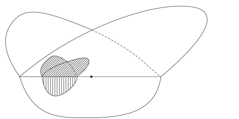
Figure 3: Pre-image of a $U_{i}$ which intersects the spine.

Now consider the pre-image $K$ of $\partial U_{i}$. Let $L_{j}$ ($1\leq j\leq 3$) be the three closed leaves of the tripod, and consider the intersection $K^{\prime}:=K\cap(L_{1}\cup L_{2})$. The set $K^{\prime}$ is the pre-image of $\partial U_{i}$ for the restriction of the map to the union $L_{1}\cup L_{2}$, hence must separate $p$ and $q$. $K^{\prime}$ is a closed subset of $L_{1}\cup L_{2}\cong\mathbb{D}^{2}$, and since $\partial U_{i}\subset I_{x}$, $K^{\prime}$ must be homeomorphic to a closed subset of $\partial U_{i}\cong S^{1}$. This implies that $K^{\prime}$ consists of either a union of intervals, or of a single $S^{1}$.

We first note that $K^{\prime}$ cannot be an $S^{1}$, for then $K^{\prime}$ would have to equal $K$ (since the map is injective on $\partial U_{i}$). One could then take a path in the third leaf joining $p$ to $q$, contradicting the fact that $K$ separates.

So we are left with dealing with the case where $K^{\prime}$ is a union of intervals. Now let $J\subset K^{\prime}$ be a subinterval that separates $p$ from $q$. Note that such an interval must exist, else $K^{\prime}$ itself would fail to separate. Now $J$ not only separates, but also locally separates $T\times\mathbb{I}$. Furthermore, $J$ cannot be contained entirely in the spine, so restricting and reparametrizing if need be, we can assume that there is a subinterval $J_{1}$ having the property that $J_{1}([0,y])\subset L_{1}$, and $J_{1}([x,1])\subset L_{2}$, where we are now viewing $J_{1}$ as a map from $\mathbb{I}$ into $L_{1}\cup L_{2}$, and $0<x\leq y<1$ (so in particular, $J_{1}([x,y])$ lies in the spine). Observe that since $J_{1}$ locally separates, we have that near $J_{1}(x)$, $L_{3}$ must map into one component of $S^{2}-\partial U_{i}$, while near $J_{1}(y)$ it must map into the other component of $S^{2}-\partial U_{i}$. This implies that there is a subinterval $J_{2}$ of $K$, lying in $L_{3}$, and separating the points near $J_{1}(x)$ from those near $J_{1}(y)$. But the union $J_{1}\cup J_{2}$ is now a subset of $K$ homeomorphic to a tripod $T$. Since $K$ is homeomorphic to a subset of $S^{1}$, this gives us a contradiction, completing the claim.

We now focus on the restriction $F_{i}$ ($1\leq i\leq 3$) of the composite map to each of the three closed leafs. Each $F_{i}$ is a map from $\mathbb{D}^{2}$ to $S^{2}$, and all three maps coincide on an interval $\mathbb{I}\subset S^{1}=\partial\mathbb{D}^{2}$ (corresponding to the spine $*\times\mathbb{I}$). From Claim 4, each of the maps $F_{i}$ is injective on $\mathbb{I}$.

Claim 5.

There is a connected open set $W\subset S^{2}$ with the property that:

• at least two of the maps $F_{i}$ surject onto $W$

• the closure of $W$ contains the point $\pi_{x}(\gamma(\infty))$

Proof.

To show this claim, we invoke the strong form of Jordan separation (Proposition 2.1). Denote by $G_{i}$ the restriction of the map $F_{i}$ to the boundary of each leaf. From the strong Jordan separation, each $G_{i}(S^{1})$ separates $S^{2}$, and there are precisely two connected open sets $U_{i},V_{i}\subset S^{2}-G_{i}(S^{1})$ which contain $G_{i}(\mathbb{I})$ in their closure. Furthermore, each of the maps $F_{i}$ surjects onto either $V_{i}$ or $U_{i}$.

Now if $r$ is small enough, we will have that the ball $D$ of radius $r$ centered at $\pi_{x}(\gamma(\infty))$ only intersects $G_{i}(\mathbb{I})$ (this follows from claim 3). In particular, each path connected component of $D-G_{i}(\mathbb{I})$ is contained in either $U_{i}$, or in $V_{i}$. Furthermore, by an argument identical to that in Proposition 2.1, there will be precisely two path connected components $U$,$V$, of $D-G_{i}(\mathbb{I})$ containing $\pi_{x}(\gamma(\infty))$ in their closure. Note that since the maps $G_{i}$ all coincide on $\mathbb{I}$, we must have (upto relabelling) $U\subset U_{i}$ and $V\subset V_{i}$ for each $i$. From the strong Jordan separation, we know that each extension $F_{i}$ surjects onto either $U_{i}$ or $V_{i}$, which implies that either $U$ or $V$ lies in the image of two of the $F_{i}$. This yields our claim.

Claim 6.

Let $V\subset S^{2}$ be a connected open set, containing the point $\pi_{x}(\gamma(\infty))$ in it’s closure. Then $V$ contains a connected open set $U_{j}$ lying in the complement of the set $I_{x}$.

Proof.

We first claim that the connected open set $V$ contains a point from $I_{x}$. Indeed, if not, then $V$ would lie entirely in the complement of $I_{x}$, hence would lie in some $U_{i}$. Since $\pi_{x}(\gamma(\infty))$ lies in the closure of $V$, it would also lie in the closure of $U_{i}$, contradicting the fact that $\gamma$ is not asymptotic to any of the boundary components of the chamber containing $\gamma$.

So not only does $V$ contain the point $\pi_{x}(\gamma(\infty))$ in its closure, it also contains some point $q$ in $I_{x}$. We claim it in fact contains a point in $I_{x}-\cup(\partial U_{i})$. If $q$ itself lies in $I_{x}-\cup(\partial U_{i})$ then we are done. The other possibility is that $q$ lies in the boundary of one of the $U_{i}$. Now since $V$ is connected, there exists a path $\eta$ joining $q$ to $\pi_{x}(\gamma(\infty))$. Now assume that $\eta\cap\big{(}I_{x}-\cup(\partial U_{i})\big{)}=\{\pi_{x}(\gamma(\infty))\}$. Let $\bar{U}_{i}$ denote the closed disks (closure of the $U_{i}$), and note that the complement of the set $I_{x}-\cup(\partial U_{i})$ is the set $\cup(\bar{U}_{i})$.

A result of Sierpinski [20] states the following: let $X$ be an arbitrary topological space, $\{C_{i}\}$ a countable collection of disjoint path connected closed subsets in $X$. Then the path connected components of $\cup C_{i}$ are precisely the individual $C_{i}$.

Applying Sierpinski’s result to the set $\cup(\bar{U}_{i})$ shows that the path connected component of this union are precisely the individual $\bar{U}_{i}$. So if $\eta\cap\big{(}I_{x}-\cup(\partial U_{i})\big{)}=\{\pi_{x}(\gamma(\infty)\}$, we see that the path $\eta$ must lie entirely within the $\bar{U}_{i}$ containing $q$. This again contradicts the fact that $\pi_{x}(\gamma(\infty))\notin\cup(\partial U_{i})$. Finally, the fact that $V$ contains a point in $I_{x}-\cup(\partial U_{i})$ allows us to invoke Claim 2, which tells us that there is some $U_{j}$ which is contained entirely within the set $V$, completing our argument.

Finally, we note that Claim 6 shows that we must have one of the connected open components $U_{j}$ of $S^{2}-I_{x}$ lying in the image of at least two distinct leaves. In particular, the boundary of the set $U_{i}$ is an $S^{1}$ which lies in the image of two distinct closed leaves. Since the boundary lies in the set of injectivity, $I_{x}$, the only way this is possible is if the spine maps to the boundary of $U_{i}$. As the map is injective on the spine, this implies that the spine $*\times\mathbb{I}$ contains an embedded copy of $S^{1}$. This gives us our contradiction, completing the proof of the proposition.

We now have to deal with the second possibility: that of geodesic rays that pass through infinitely many connected lifts $\tilde{W}_{i}$. We start by proving a few lemmas concerning separability properties for the $\tilde{B}_{i}$ and $\tilde{W}_{i}$, which will also be usefull for our applications.

Lemma 2.1.

Let $\tilde{B}_{i}$ be a connected lift of the branching locus, and let $\tilde{W}_{j}$, $\tilde{W}_{k}$ be two lifts of chambers which are both incident to $\tilde{B}_{i}$. Then $\tilde{W}_{j}-\tilde{B}_{i}$ and $\tilde{W}_{k}-\tilde{B}_{i}$ lie in different connected components of $\tilde{X}^{3}-\tilde{B}_{i}$.

Proof.

We start with a trivial observation, which will be crucial in the proof of both this lemma and the following one. Take any cyclic sequence $\tilde{W}_{0},\tilde{B}_{0},\tilde{W}_{1},\tilde{B}_{1},\ldots,\tilde{W}_{r},\tilde{B}_{r}$ of distinct connected lifts of chambers and branching locus with the property that each term is incident to the following one. Then the union of all these sets forms a totally geodesic subset of $\tilde{X}^{3}$. Furthermore, by a simple application of Seifert-Van Kampen, we find that this totally geodesic subset of a simply connected non-positively curved space has $\pi_{1}\cong\mathbb{Z}$. But this is impossible, so no such sequence can exist.

Now, assume that we have two lifts of chambers $\tilde{W}_{j}$, $\tilde{W}_{k}$ which are both incident to a connected lift $\tilde{B}_{i}$, but which lie in the same connected component of $\tilde{X}^{3}-\tilde{B}_{i}$. Then taking a geodesic joining a point in $\tilde{W}_{j}$ to a point in $\tilde{W}_{k}$ but not intersecting $\tilde{B}_{i}$, we can consider the sequence of (connected lifts of) chambers and branching locus that the geodesic passes through to get a sequence as above. But as we explained, this gives us a contradiction.

Lemma 2.2.

Let $\tilde{W}_{i}$ be a connected lift of a chamber, and let $\tilde{B}_{j}$, $\tilde{B}_{k}$ be two connected lifts of the branching locus which are both incident to $\tilde{W}_{i}$. Then $\tilde{B}_{j}$ and $\tilde{B}_{k}$ lie in different connected components of $\tilde{X}^{3}-Int(\tilde{W}_{I})$.

Proof.

This proof is identical to the previous one: just interchange the roles of the connected lifts of chambers and the connected lifts of the branching locus.

Next, we note that, in the setting we are considering, we can push the separability properties out to infinity, obtaining that the corresponding boundary points separate.

Lemma 2.3.

Let $\partial^{\infty}\tilde{B}_{i}$ be the boundary at infinity of a connected lift of the branching locus, and let $\partial^{\infty}\tilde{W}_{j}$, $\partial^{\infty}\tilde{W}_{k}$ be the boundaries at infinity of two lifts of chambers which are both incident to $\tilde{B}_{i}$. Then $\partial^{\infty}\tilde{W}_{j}-\partial^{\infty}\tilde{B}_{i}$ and $\partial^{\infty}\tilde{W}_{k}-\partial^{\infty}\tilde{B}_{i}$ lie in different connected components of $\partial^{\infty}\tilde{X}^{3}-\partial^{\infty}\tilde{B}_{i}$.

Proof.

Let $\eta:[0,1]\longrightarrow\partial^{\infty}\tilde{X}^{3}$ be a path in the boundary at infinity joining a point in $\partial^{\infty}\tilde{W}_{j}-\partial^{\infty}\tilde{B}_{i}$ to a point in $\partial^{\infty}\tilde{W}_{k}-\partial^{\infty}\tilde{B}_{I}$, which avoids $\partial^{\infty}\tilde{B}_{i}$. Fix a basepoint $p\in\tilde{B}_{i}$, and consider the pair of geodesics $\gamma_{i}:[0,\infty)\longrightarrow\tilde{X}^{3}$ ($i=0,1$) satisfying $\gamma_{i}(0)=p$, and $\gamma_{i}(\infty)=\eta(i)$.

Now observe that, by assumption, $\eta([0,1])\cap\partial^{\infty}\tilde{B}_{i}=\emptyset$, and as they are both compact subsets, this forces $d_{\infty}(\eta([0,1]),\partial^{\infty}\tilde{B}_{i})>\epsilon>0$. So let us consider a covering of $\eta([0,1])$ by open balls of radius $r=\epsilon/4$ in the compactification $\tilde{X}^{3}\cup\partial^{\infty}\tilde{X}^{3}$. Note that these open balls are all path-connected. By compactness of $\eta$, we can extract a finite subcover $\{U_{i}\}$ which still covers $\eta$. The union of these open sets form a neighborhood of $\eta$ in the compactification, which, by our choice of $r$ cannot intersect $\tilde{B}_{i}$. Furthermore, this neighborhood is connected, and for sufficiently large $t$, both $\gamma_{0}(t)$ and $\gamma_{1}(t)$ lie in the neighborhood. By concatenation of paths, we can obtain a path $\gamma$ which completely avoids $\tilde{B}_{i}$, but joins a point in $\tilde{W}_{i}$ to a point in $\tilde{W}_{j}$. However, we have already shown that the latter two subsets lie in distinct path components of $\tilde{X}^{3}-\tilde{B}_{i}$. Our claim follows.

Lemma 2.4.

Let $\partial^{\infty}\tilde{W}_{i}$ be the boundary at infinity corresponding to a connected lift of a chamber, and let $\partial^{\infty}\tilde{B}_{j}$, $\partial^{\infty}\tilde{B}_{k}$ be the boundary at infinity of two connected lifts of the branching locus which are both incident to $\tilde{W}_{i}$. Then $\partial^{\infty}\tilde{B}_{j}$ and $\partial^{\infty}\tilde{B}_{k}$ lie in different connected components of $\partial^{\infty}\tilde{X}^{3}-(\partial^{\infty}\tilde{W}_{i}-\cup\partial^{\infty}\tilde{B}_{l})$, where the union is over all $\tilde{B}_{l}$ which are boundary components of $\tilde{W}_{i}$.

Proof.

Let us start by noting that all of the sets $\partial^{\infty}\tilde{B}_{j}$ are closed subsets of $\partial^{\infty}\tilde{X}^{3}$. Let us focus on those $\tilde{B}_{l}$ which are the boundary of our $\tilde{W}_{i}$. By our previous result, each of those separates within $\tilde{X}^{3}$. So for each of them, we can consider the union of the components which do not contain $\tilde{W}_{i}$. Together with the corresponding $\tilde{B}_{l}$, these will form a countable family of closed totally geodesic subsets $C_{l}$ indexed by the boundary components of $\tilde{W}_{i}$. Consider the corresponding subsets $\partial^{\infty}C_{l}$ in $\partial^{\infty}\tilde{X}^{3}$. Since each of these $C_{l}$ is totally geodesic, the corresponding subset $\partial^{\infty}C_{l}$ is a closed subset of $\partial^{\infty}\tilde{X}^{3}$. Furthermore, their union is the whole of $\partial^{\infty}\tilde{X}^{3}-(\partial^{\infty}\tilde{W}_{i}I-\cup\partial^{\infty}\tilde{B}_{l})$. We now claim that the sets $\partial^{\infty}C_{l}$ are pairwise disjoint. But this is clear: by construction, we have that the $\partial^{\infty}\tilde{B}_{l}$ separate $\partial^{\infty}C_{l}$ from all the other $\partial^{\infty}C_{k}$. So the distance from any point $p\in\partial^{\infty}C_{l}$ to any point $q\in\partial^{\infty}C_{k}$ is at least as large as the distance between the corresponding $\partial^{\infty}\tilde{B}_{l}$ and $\partial^{\infty}\tilde{B}_{k}$. But since the two totally geodesic subsets $\tilde{B}_{l}$ and $\tilde{B}_{k}$ diverge exponentially, the sets $\partial^{\infty}\tilde{B}_{l}$ and $\partial^{\infty}\tilde{B}_{k}$ are some positive distance apart.

Finally, let us assume there is some path $\eta:\mathbb{I}\longrightarrow\partial^{\infty}\tilde{X}^{3}$ satisfying $\eta(0)\in\partial^{\infty}\tilde{B}_{j}$, $\eta(1)\in\partial^{\infty}\tilde{B}_{k}$ ($j\neq k$), and $\eta\cap\partial^{\infty}\tilde{W}_{i}=\emptyset$. Then $\eta$ is a continuous map that lies entirely in the complement of $\partial^{\infty}\tilde{W}_{i}$. Consider the pre-image of the various closed sets $\partial^{\infty}\tilde{C}_{r}$ under $\eta$. This provides a covering of the unit interval by a countable family of disjoint closed sets. Applying the result of Sierpinski [20] which was stated in the proof of Proposition 2.2 (Claim 6), this is impossible unless the covering is by a single set, consisting of a single interval. This concludes our argument.

Note that the previous two lemmas allow us to identify separability properties within the space with separability properties on the boundary at infinity. In particular, we can talk about a point within the space lying in a different component from a point at infinity (i.e. the unique geodesic joining the pair of points intersects the totally geodesic separating subset, whether this is a $\tilde{B}_{i}$ or a $\tilde{W}_{i}$). We are now ready to deal with the second case of theorem 1.1:

Proposition 2.3.

Let $X^{3}$ be a simple, thick 3-dimensional hyperbolic P-manifold. Let $\gamma\subset\tilde{X}^{3}$ be a geodesic that passes through infinitely many connected lifts $\tilde{W}_{i}$. Then $\gamma(\infty)$ is not 2-branching.

Proof.

The approach here consists of reducing to the situation covered in proposition 2.2. We start by re-indexing the various consecutive connected lifts $\tilde{W}_{i}$ that $\gamma$ passes through by the integers. Fix a basepoint $x\in\tilde{W}_{0}$ interior to the connected lift $\tilde{W}_{0}$, and lying on $\gamma$. Now assume that there is an injective map $f:T\times\mathbb{I}\longrightarrow\partial^{\infty}\tilde{X}^{3}$ with $\gamma(\infty)\in f(*\times\mathbb{I}_{\circ})$.

We start by noting that, between successive connected lifts $\tilde{W}_{i}$ and $\tilde{W}_{i+1}$ that $\gamma$ passes through, lies a connected lift of the branching locus, which we denote $\tilde{B}_{i}$. Observe that distinct connected lifts of the branching locus stay a uniformly bounded distance apart. Indeed, any minimal geodesic joining two distinct lifts of the branching locus must descend to a minimal geodesic in a $W_{i}$ with endpoints in the branching locus. But the length of any such geodesic is bounded below by half the injectivity radius of $DW_{i}$, the double of $W_{I}$ across its boundary. By setting $\delta$ to be the infimum, over all the finitely many chambers $W_{i}$, of the injectivity radius of the doubles $DW_{i}$, we have $\delta>0$. Let $K_{i}$ be the connected component of $\partial^{\infty}\tilde{X}^{3}-\partial^{\infty}\tilde{B}_{i}$ containing $\gamma(\infty)$. Then for every $p\in K_{i}$ ($i\geq 1$), we have:

$$d_{x}(p,\gamma(\infty))<e^{-\delta(i-1)}.$$

Indeed, by Lemma 2.1, $\tilde{B}_{i}$ separates $\tilde{X}^{3}$ into (at least) two totally geodesic components. Furthermore, the component containing $\gamma(\infty)$ is distinct from that containing $x$. Hence, the distance from $x$ to the geodesic joining $p$ to $\gamma(\infty)$ is at least as large as the distance from $x$ to $\tilde{B}_{i}$. But the later is bounded below by $\delta(i-1)$. Using the definition of the metric at infinity, and picking $x$ as our basepoint, our estimate follows.

Since our estimate shrinks to zero, and since the distance from $\gamma(\infty)$ to $f(\partial(T\times\mathbb{I}))$ is positive, we must have a point $q\in f(*\times\mathbb{I}_{\circ})$ satisfying $d_{x}(q,\gamma(\infty))>e^{-\delta(i-1)}$ for $i$ sufficiently large. Since $\tilde{B}_{i}$ separates, we see that for $i$ sufficiently large, $f(*\times\mathbb{I}_{\circ})$ contains points on both sides of $\partial^{\infty}\tilde{B}_{i}$. This implies that there is a point $q^{\prime}\in f(*\times\mathbb{I}_{\circ})$ that lies within some $\partial^{\infty}\tilde{W}_{k}$. But such a point corresponds to a geodesic ray lying entirely within $\tilde{W}_{k}$, and not asymptotic to any of the lifts of the branching locus. Finally, we note that any point in the image $f(*\times\mathbb{I}_{\circ})$ can be considered $2$-branching, so in particular the point $q^{\prime}$ is $2$-branching. But in the previous proposition, we showed this is impossible. Our claim follows.

Combining propositions 2.1, 2.2, and 2.3 gives us the result claimed in theorem 1.1. We round out this section by making a simple observation, which will be used in the proofs of theorem 1.2 and 1.3.

Lemma 2.5.

Let $X^{n}$ be a simple hyperbolic P-manifold of dimension at least three Let $\partial^{\infty}\tilde{B}\subset\partial^{\infty}\tilde{X}^{n}$ consist of all limit points of geodesics in the branching locus. If $n\geq 3$, then the maximal path-connected components of $\partial^{\infty}\tilde{B}$ are precisely the sets of the form $\partial^{\infty}\tilde{B}_{i}$, where $\tilde{B}_{i}\subset\tilde{B}$ is a single connected component of the lifts of the branching locus.

Proof.

Clearly, the sets $\partial^{\infty}\tilde{B}_{i}$ are closed (since the $\tilde{B}_{i}$ are totally geodesic) and path-connected (since each $\tilde{B}_{i}$ is an isometrically embedded $\mathbb{H}^{n-1}$, so the corresponding $\partial^{\infty}\tilde{B}_{i}\cong S^{n-2}$). Now let $\tilde{B}_{i},\tilde{B}_{j}$ be distinct connected components of $\tilde{B}$. We are left with showing that $\partial^{\infty}\tilde{B}_{i}\cap\partial^{\infty}\tilde{B}_{j}=\emptyset$. Consider a geodesic $\gamma$ joining $\tilde{B_{i}}$ to $\tilde{B_{j}}$. Since they are distinct connected lifts of the branching locus, this geodesic must intersect a $\tilde{W}_{k}$. By lemma 2.4, a proper subset of $\partial^{\infty}\tilde{W}_{k}$ separates $\partial^{\infty}\tilde{B}_{i}$ from $\partial^{\infty}\tilde{B}_{j}$. In particular, this forces the latter two sets to be disjoint. To conclude, we apply the result of Sierpinski [20] (stated in the proof of Proposition 2.2, Claim 6). This concludes the proof of the Lemma.

3 Applications: rigidity results.

3.1 Mostow rigidity and consequences.

In this section, we provide a proof of Mostow rigidity for simple, thick, hyperbolic P-manifolds of dimension $3$ (Theorem 1.2). We also mention some immediate consequences of the main theorem.

Proof.

We are given a pair $X_{1}$, $X_{2}$ of simple, thick, hyperbolic P-manifolds of dimension $3$, with isomorphic fundamental groups, and we want to show that the two spaces are isometric. We start by noting that our isomorphism of the fundamental groups is a quasi-isometry, so that we get an induced homeomorphism $\partial^{\infty}\Phi:\partial^{\infty}\tilde{X}_{1}\longrightarrow\partial^{\infty}\tilde{X}_{2}$ between the boundaries at infinity of the two universal covers $\tilde{X}_{1}$ and $\tilde{X}_{2}$. Let $Y_{1}\subset\partial^{\infty}\tilde{X}_{1}$, $Y_{2}\subset\partial^{\infty}\tilde{X}_{2}$ be the set of points in the respective boundaries at infinity that are $2$-branching. Note that since $\partial^{\infty}\Phi$ is a homeomorphism, and since the property of being $2$-branching is a topological invariant, we must have $(\partial^{\infty}\Phi)(Y_{1})=Y_{2}$. Let $B_{1,i}\subset\tilde{X}_{1}$, $B_{2,i}\subset\tilde{X}_{2}$ be the various connected lifts of the branching locus.

Theorem 1.1 tells us that we have the equalities $Y_{1}=\bigcup(\partial^{\infty}\tilde{B}_{1,i})$, $Y_{2}=\bigcup(\partial^{\infty}\tilde{B}_{2,i})$. In particular, $\partial^{\infty}\Phi$ must map each path connected component of $Y_{1}$ to a path connected component of $Y_{2}$. This implies (by Lemma 2.5) that $\partial^{\infty}\Phi$ induces a bijection between the lifts $\tilde{B}_{1,i}$ and the lifts $\tilde{B}_{2,i}$. Furthermore, the homeomorphism $\partial^{\infty}\Phi$ must map the complement of the set $Y_{1}$ to the complement of the set $Y_{2}$. Note that in $\partial^{\infty}\tilde{X}_{1}$ and $\partial^{\infty}\tilde{X}_{2}$, the complements of the sets $Y_{1}$, $Y_{2}$ will have path components of the following two types:

1. path-isolated points, corresponding to geodesic rays that pass through infinitely many $\tilde{W}_{i}$, and

2. non-path-isolated points, corresponding to geodesic rays that eventually lie entirely within a fixed $\tilde{W}_{i}$ (and are not asymptotic to a boundary component).

We note that there are uncountably many of the former, but only countably many path connected components of the latter. In particular, our homeomorphism cannot map a non-isolated point to an isolated point. Hence our homeomorphism provides us with a bijection from the set of connected lifts of chambers in $\tilde{X}_{1}$ to the set of connected lifts of chambers in $\tilde{X}_{2}$.

The next claim is that if a lift of a chamber $\tilde{W}_{1}\subset\tilde{X}_{1}$ corresponds to a lift of a chamber $\tilde{W}_{2}\subset X_{2}$, that they are in fact isometric. To see this, we consider the chamber $W_{1}\subset X_{1}$,$W_{2}\subset X_{2}$ whose lifts we are dealing with, and note that they have isomorphic fundamental groups. Indeed, consider the action of the fundamental groups of the two P-manifolds on their boundary at infinity. Then the fundamental group of a chamber $W_{i}$ can be identified with the stabilizer of $\tilde{W}_{i}$ for the action of $\pi_{1}(X_{1})$ as deck transformations. We would like to identify $\pi_{1}(W_{i})$ from the boundary at infinity. This is the content of the following:

Assertion: The stabilizer of the lift of a chamber $\tilde{W}_{i}$ coincides with the stabilizer of the set $\partial^{\infty}\tilde{W}_{i}$ in the boundary at infinity. The respective actions are those of $\pi_{1}(X)$ as deck transformations on $\tilde{X}$, and the corresponding induced action on the boundary at infinity.

To see this, we note that the stabilizer of $\tilde{W}_{i}$ will clearly stabilize $\partial^{\infty}\tilde{W}_{i}$. Conversely, assume that we have a non-trivial element $\alpha$ in $\pi_{1}(X)$ which stabilizes $\partial^{\infty}\tilde{W}_{i}$. Note that, the $\tilde{B}_{i}$ must be permuted by any isometry, and from Lemma 2.1 they separate $\tilde{X}$ into the various lifts of chambers. Hence it is sufficient to exhibit a point in $\tilde{W}_{i}$ whose image under $\alpha$ is also in $\tilde{W}_{i}$.

Note that if $\alpha$ stabilizes $\partial^{\infty}\tilde{W}_{i}$, then so do all its powers. Since $\alpha$ acts hyperbolically on the boundary at infinity, this implies that the sink/source of the $\alpha$ action lies in the set $\partial^{\infty}\tilde{W}_{i}$. Hence $\alpha$ stabilizes a geodesic $\gamma$ lying entirely in $\tilde{W}_{i}$ (joining the sink and source of the $\alpha$ action on the boundary at infinity). There are now two possibilities: either $\gamma$ lies in the interior of $\tilde{W}_{i}$ and we are done, or $\gamma$ lies on the boundary. If $\gamma$ lies on the boundary, then we have that $\alpha$ must stabilize that boundary component, call it $\tilde{D}$. Now pick a point $q$ in $\partial^{\infty}\tilde{W}_{i}$ which is not on $\partial^{\infty}\tilde{D}$, and let $\eta$ be a geodesic from a point in $D$ to the point $q$. Since $\alpha$ stabilizes $D$, and stabilizes $\partial^{\infty}\tilde{W}_{i}$ it maps $\eta$ to a geodesic ray emanating from a point in $D$, and having endpoint not on $\partial^{\infty}\tilde{D}$. In particular, $\alpha$ maps a point in the interior of $\tilde{W}_{i}$ (namely an interior point on the ray $\eta$) to another interior point. As we remarked earlier, this implies that $\alpha$ stabilizes $\tilde{W}_{i}$, giving us the assertion.

From the assertion, we now have the desired claim that if $\tilde{W}_{1}\subset\tilde{X}_{1}$ corresponds to a $\tilde{W}_{2}\subset\tilde{X}_{2}$, then the chambers $W_{1}$ and $W_{2}$ have isomorphic fundamental groups. Mostow rigidity for hyperbolic manifolds with boundary (see Frigerio [7]) now allows us to conclude that the $W_{1}$ is isometric to $W_{2}$, and that the isometry induces the isomorphism given above. Lifting this isometry, we see that there is an isometry of $\tilde{W}_{1}$ to $\tilde{W}_{2}$ which induces the isomorphism between the two respective stabilizers.

Next we discuss how the isometries on the lift of the chambers glue together to give a global isometry. We first need to ensure that adjacent chambers in $X_{1}$ map to adjacent chambers in $X_{2}$. Note that two chambers in $X_{1}$ are adjacent if and only if there is a unique $B_{1,i}$ separating them. But by Lemma 2.3, this can be detected on the level of the boundary at infinity. Since the $B_{1,i}$ map bijectively to the $B_{2,i}$, there will be a unique $B_{1,i}$ separating a pair of chambers if and only if there is a unique $B_{2,i}$ separating the corresponding chambers in $X_{2}$. This implies that incident chambers map to incident chambers. Finally, we can recognize the fundamental group of the common codimension one manifold $B_{i}$ in terms of the sink/source dynamics of the action of the fundamental group of each chamber on the corresponding boundary component. This also allows us to recognize the subgroups of the $\pi_{1}(W_{1,i})$ and $\pi_{1}(W_{1,j})$ that get identified. Equivariance of the homeomorphism ensures that the corresponding image groups get identified in precisely the same way, which implies that the corresponding lifts of the chambers are glued together in an equivariant, isometric manner. Finally, we see that there is an equivariant isometry between the universal covers $\tilde{X}_{1}$ and $\tilde{X}_{2}$, which gives us our desired claim. It is clear from our construction that the isometry we obtain induces the original isomorphism between the fundamental groups.

We point out two immediate (and standard) corollaries:

Corollary 3.1.

Let $X^{3}$ be a simple, thick hyperbolic P-manifold of dimension $3$, $\Gamma$ its fundamental group. Then the outer automorphism group $Out(\Gamma)$ is a finite group, isomorphic to $Isom(X^{3})$ (the isometry group of the P-manifold).

Corollary 3.2.

Let $X^{3}$ be a simple, thick hyperbolic P-manifold of dimension $3$, $\Gamma$ its fundamental group. Then $\Gamma$ is a co-Hopfian group.

Concerning corollary 3.1, we remark that Paulin [16] has shown that a $\delta$-hyperbolic group with infinite outer automorphism group splits over a virtually cyclic group. As for corollary 3.2, we point out that Sela has shown that torsion-free $\delta$-hyperbolic groups are Hopfian [18], and that a non-elementary torsion-free $\delta$-hyperbolic group is co-Hopfian if and only if it is freely indecomposable [17].

Now let $\Sigma_{3}$ consist of those groups which arise as the fundamental group of a simple, thick hyperbolic P-manifold of dimension $3$. Note that every group in $\Sigma_{3}$ arises as the fundamental group of a graph of groups, induced by the decomposition of the P-manifold into its chambers (see Serre [19] for definitions). Furthermore, the gluings between the chambers are encoded in the morphisms attached to each edge in the graph of groups. A purely group theoretic reformulation of Mostow rigidity is the following:

Corollary 3.3 (Diagram Rigidity).

Let $H_{1},H_{2}$ be groups in $\Sigma_{3}$. Then $H_{1}\cong H_{2}$ if and only if there is an isomorphism between the underlying graph of groups with the property that:

• the isomorphism takes vertex groups to isomorphic vertex groups,

• isomorphisms can be chosen between the vertex groups which intertwine all the edge morphisms.

This result essentially asserts that the “structure” of the graph of groups that yield groups in $\Sigma_{3}$ is in fact unique. For related results, we refer to Forester [8] (see also Guirardel [11]).

3.2 Quasi-isometry rigidity.

In this section, we provide a proof of Theorem 1.3, giving a quasi-isometry classification for fundamental groups of simple, thick hyperbolic P-manifolds of dimension $3$. In proving this theorem, we will use the following well known result (for a proof, see Proposition 3.1 in Farb [6]):

Lemma 3.1.

Let $X$ be a proper geodesic metric space, and assume that every quasi-isometry from $X$ to itself is in fact a bounded distance from an isometry. Furthermore, assume that a finitely generated group $G$ is quasi-isometric to $X$. Then there exists a cocompact lattice $\Gamma\subset Isom(X)$, and a finite group $F$ which fit into a short exact sequence:

$$0\longrightarrow F\longrightarrow G\longrightarrow\Gamma\longrightarrow 0$$

So to prove the theorem, it is sufficient to show that any quasi-isometry of a simple, thick P-manifold of dimension $3$ is a bounded distance away from an isometry. In order to do this, we begin by recalling a well known “folklore” result. Proofs of this have been given at various times by Farb, Kapovich, Kleiner, Leeb, Schwarz, Wilkinson, and others, though no published proof exists (both B. Kleiner and B. Farb were kind enough to e-mail us their arguments, which we sketch out below).

Proposition 3.1.

Let $M^{3}$ be a compact hyperbolic 3-manifold with totally geodesic boundary (non-empty). Then any quasi-isometry of the universal cover $\tilde{M}^{3}$ is a finite distance from an isometry.

The idea of the argument is to repeatedly reflect $\tilde{M}^{3}$ through the totally geodesic boundary components to get a copy of $\mathbb{H}^{3}$, tiled by copies of $\tilde{M}^{3}$. Now given a quasi-isometry of the original $\tilde{M}^{3}$, we can extend to a quasi-isometry of all of $\mathbb{H}^{3}$, which has the special property that it preserves the union of the boundaries (as sets). This quasi-isometry extends to a quasi-conformal homeomorphism of the boundary $S^{2}$ that interchanges certain families of $S^{1}$ (the points at infinity corresponding to the various boundaries). Using the fact that this homeomorphism preserves a family of circles containing nested circles of arbitrarily small size, one shows that the quasi-conformal homeomorphism is in fact conformal. This implies that there is an isometry of $\mathbb{H}^{3}$ which is bounded distance from the original quasi-isometry. Furthermore, by construction, this isometry preserves our original $\tilde{M}^{3}$.

Now assuming the preceding folklore theorem, we proceed to give a proof of Theorem 1.3:

Proof.

Let us start by showing our first claim: that any quasi-isometry of the universal cover $\tilde{X}$ of a simple, thick P-manifold $X$ of dimension $3$ lies a finite distance away from an isometry. Notice that our quasi-isometry induces a self-homeomorphism of the boundary at infinity $\partial^{\infty}\tilde{X}$. Once again, Theorem 1.1 implies that the induced map on the boundary at infinity acts as a permutation on the set of boundaries of connected lifts of the branching locus.

In particular, this forces our quasi-isometry to map each of the branching strata $\tilde{B}_{i}$ inside the P-manifold to within finite distance of another branching strata, call it $\tilde{B}_{i}^{\prime}$. Since under a quasi-isometry we have uniform control of the distance between the images of geodesics and actual geodesics, we see that there is a uniform upper bound on the distance between the image of $\tilde{B}_{i}$ and the strata $\tilde{B}_{i}^{\prime}$. As such, we can modify our quasi-isometry by projecting the images of each $\tilde{B}_{i}$ to the corresponding $\tilde{B}_{i}^{\prime}$. Since this projection only moves points by a bounded distance, we have that the new map is still a quasi-isometry, and is bounded distance from the one we started with.

So we have now reduced to the case where the quasi-isometry maps each $\tilde{B}_{i}$ into the corresponding $\tilde{B}_{i}^{\prime}$. Since our induced homeomorphism on the boundary also permutes the boundaries of the $\tilde{W}_{i}$, we can apply the same projection argument to ensure that our new quasi-isometry actually maps each $\tilde{W}_{i}$ strictly into a corresponding $\tilde{W}_{i}^{\prime}$. Let us denote this new quasi-isometry by $f$. Now Proposition 3.1 forces $\tilde{W}_{i}\cong\tilde{W}_{i}^{\prime}$, and the restriction of our quasi-isometry $f$ to $\tilde{W}_{i}$ is a bounded distance from an isometry $\phi_{i}:\tilde{W}_{i}\longrightarrow\tilde{W}_{i}^{\prime}$. Furthermore, as in our proof of Mostow rigidity, a separation argument ensures that incidence of the chambers $\tilde{W}_{i}$,$\tilde{W}_{j}$ forces the corresponding chambers $\tilde{W}_{i}^{\prime}$ and $\tilde{W}_{j}^{\prime}$ to be incident.

We now want to get a global isometry from the isometries on chambers. Observe that, for an incident pair of chambers $\tilde{W}_{i}$ and $\tilde{W}_{j}$, we can consider the branching strata $\tilde{W}_{i}\cap\tilde{W}_{j}$. The image of this map under $f$ is $\tilde{W}_{i}^{\prime}\cap\tilde{W}_{j}^{\prime}\cong\mathbb{H}^{2}$. Furthermore, we have a pair of isometries $\phi_{i},\phi_{j}$ from $\tilde{W}_{i}\cap\tilde{W}_{j}$ to $\tilde{W}_{i}^{\prime}\cap\tilde{W}_{j}^{\prime}$, each of which is a finite distance from the map $f$, so in particular, which must be a finite distance from each other. Considering the isometry $g:=\phi_{j}^{-1}\circ\phi_{i}:\tilde{W}_{i}\cap\tilde{W}_{j}\longrightarrow\tilde{W}_{i}\cap\tilde{W}_{j}$, we obtain an isometry of $\tilde{W}_{i}\cap\tilde{W}_{j}$ which is bounded distance from the identity. But the only isometry of $\mathbb{H}^{2}$ which is bounded distance from the identity is the identity itself. This allows us to conclude that $\phi_{i}$ and $\phi_{j}$ are exactly the same isometry when restricted to $\tilde{W}_{i}\cap\tilde{W}_{j}$, allowing us to glue them together. Since this holds for arbitrary incident chambers, we can combine all the various isometries into a globally defined isometry on $\tilde{X}$.

We are left with showing that the resulting isometry is a bounded distance from the original quasi-isometry. Note that, for the time being, we only know that on each lift of a chamber $\tilde{W}_{i}$ the isometry is bounded distance $D_{i}$ from an isometry. We still need to deal with the possibility that the individual $D_{i}$ might be tending to infinity.

This prompts the question: given that a $(C,K)$-quasi-isometry is a bounded distance from an isometry, can we obtain a uniform upper bound on how large this distance can get? We need to obtain a uniform bound for quasi-isometries of the universal cover of compact hyperbolic manifolds with (non-empty) totally geodesic boundary.

In order to answer this, we recall that, for an arbitrary $(C,K)$ quasi-isometry $f$ on a $CAT(\delta)$ space $\tilde{W}$ ($\delta<0$), there is a uniform constant $D:=D_{C,K,\delta}$ (depending solely on the constants $C,K,\delta$) with the following property. Given any bi-infinite geodesic $\gamma$, the distance between the image $f(\gamma)$ (which is referred to as a quasi-geodesic) and the bi-infinite geodesic with endpoints $\partial^{\infty}f(\gamma(\pm\infty))$ is bounded above by $D$. Naturally, if the quasi-isometry is bounded distance from an isometry $\phi$, then the latter geodesic is precisely $\phi(\gamma)$.

Now let us assume that we are dealing with a space with the property that every point has a pair of perpendicular bi-infinite geodesics $\gamma_{1},\gamma_{2}$ intersecting precisely in $p$. We will abbreviate this property to saying that a space has (PBIG). Then for our isometry, we see that $\phi(p)=\phi(\gamma_{1})\cap\phi(\gamma_{2})$, while for our quasi-isometry we only obtain $f(p)\subset f(\gamma_{1})\cap f(\gamma_{2})$. Since $f(\gamma_{i})$ lies in the $D$ neighborhood of $\phi(\gamma_{i})$, we see that $f(p)$ lies in the intersection of the $D$-neighborhoods of a pair of intersecting geodesics, which, since $\phi$ is an isometry, are in fact perpendicular geodesics. But such a neighborhood has a diameter that is uniformly bounded by some constant $D^{\prime}$ which only depends on $D$ (and hence on $C,K,\delta$).

Note that the spaces we are interested in are universal covers of compact hyperbolic manifolds with non-empty boundary, so it is not clear that the above property holds. It is easy to see that every point is contained in a bi-infinite geodesic, but it is less clear that one can find two such geodesics which are perpendicular. For the spaces we are considering, we now make the:

Assertion: There exists a constant $D^{\prime\prime}$ with the property that if $\gamma$ is an inextendable geodesic, then $d(f(\gamma),\phi(\gamma))\leq D^{\prime\prime}$.

Assuming this assertion, it is easy to obtain the upper bound we desire. Indeed, every point in $\tilde{W}$ is the intersection of a pair of perpendicular inextendable geodesics $\gamma_{1},\gamma_{2}$ (which either terminate at the boundary, or extend off to infinity). The same argument as before shows that $f(p)$ must lie in the intersection of the $D^{\prime\prime}$ neighborhoods of $\phi(\gamma_{1})$ and $\phi(\gamma_{2})$, giving uniform control of $d(f(p),\phi(p))$

To see that the desired assertion is true, we note that we only have to deal with geodesic segments with both endpoints on boundary components, or geodesic rays emanating from a boundary component (the case of bi-infinite geodesics having been discussed above). Now note that, since the boundary components have the property (PBIG) (indeed, they are totally geodesic $\mathbb{H}^{2}$’s), we have that for points $q$ on the boundary components, $d(f(q),\phi(q))\leq D^{\prime}$.

If $\gamma$ is a geodesic segment with both endpoints $q_{1},q_{2}$ on boundary components, then we have that $d(f(\gamma),\eta)\leq D$, where $\eta$ is the geodesic joining $f(q_{1})$ to $f(q_{2})$. However, we also have that $d(f(q_{i}),\phi(q_{i}))\leq D^{\prime}$, so by convexity of the distance function $d(\eta,\nu)\leq D^{\prime}$, where $\nu$ is the geodesic joining $\phi(q_{1})$ to $\phi(q_{2})$. But that geodesic is precisely $\phi(\gamma)$, so the triangle inequality yields $d(\phi(\gamma),f(\gamma))\leq D+D^{\prime}=:D^{\prime\prime}$, giving the desired upper bound for this case. The case of a geodesic ray with endpoint on a boundary component follows from an identical argument.

We conclude that we have the desired uniform bound, which implies that our gluing of the ‘piecewise’ isometries is still a bounded distance from an isometry.

Now a consequence of every quasi-isometry being finite distance from an isometry is that any group $G$ quasi-isometric to $H$ must fit into a short exact sequence:

$$0\longrightarrow F\longrightarrow G\longrightarrow\Gamma\longrightarrow 0$$

where $F$ is a finite group and $\Gamma\subset Isom(\tilde{X})$ (see Lemma 3.1). The theorem follows.

For other recent results on the quasi-isometry behavior of graphs of groups, we refer to Papasoglu [14], Papasoglu-Whyte [15], and Mosher-Sageev-Whyte [13].

4 Concluding remarks.

We note that the only place in our arguments where we use the assumption that $n=3$ is in the proof of the strong Jordan separation theorem. More specifically, we make use of the fact that the Schoenflies theorem holds in dimension $2$. Of course, this approach fails in higher dimension, as there are examples of wild embeddings of spheres in all dimensions $\geq 3$. Nevertheless, we still believe that the conjecture put forth in the introduction holds true (and in fact, that the strong Jordan separation theorem also holds in higher dimension).

A more general question would be to determine which hyperbolic P-manifolds exhibit rigidity. One would need some sort of hypotheses, as the following example shows:

Example: Let $X_{i}$ ($1\leq i\leq 3$) be simple, thick, hyperbolic P-manifolds of dimension $3$. In each $X_{i}$, let $Y_{i}\subset X_{i}$ be one of the surfaces in the $2$-dimensional strata, and let $\gamma_{i}$ be a simple closed geodesic in each $Y_{i}$. We now propose to build a thick, hyperbolic P-manifold which is not rigid. Let $G$ be a complete graph on four vertices, and $T_{i}$ be three triangles in $G$. Assign a length to each edge in such a way that the triangles $T_{i}$ have length equal to the corresponding $\gamma_{i}$.

Note that given isometries from $\gamma_{i}$ to $T_{i}$, we can form a thick, hyperbolic P-manifold by gluing the $X_{i}$ to $G$ by identifying the $\gamma_{i}$ with the $T_{i}$. Furthermore, as long as the gluing isometries are homotopic, the resulting P-manifolds will all have isomorphic fundamental group. So provided we can find two different gluings which yield non-isometric P-manifolds, we will have exhibited non-rigidity.

To do this, fix the gluing of $X_{2}$, $X_{3}$, and ‘rotate’ the gluing map for the $X_{1}$. Note that, in the surface $Y_{1}$, there are countably many geodesic segments which are perpendicular to $\gamma_{1}$ and intersect $\gamma_{1}$ precisely at their endpoints. By rotating the gluing map suitably, we can ensure that one of the resulting P-manifolds has such a geodesic segment in $Y_{1}$ emanating from a vertex of the triangle $T_{1}$, whereas another one of the resulting P-manifolds does not. It is now clear that these two P-manifolds cannot be isometric, despite the fact that they have isomorphic fundamental groups. Observe that these examples will have a non-trivial one-dimensional strata (namely the graph $G$), so do not satisfy the simplicity hypothesis of this paper.

Note that if there is no 1-dimensional strata, one cannot use the ‘rotation trick’ to get counterexamples (since the isometry group of compact hyperbolic manifolds is finite if the dimension is at least two). Perhaps the following is reasonable:

Question: Is every hyperbolic P-manifold with empty 1-dimensional strata Mostow rigid?

Other interesting questions arise from trying to further understand the (full) group of isometries $Isom(\tilde{X})$ of the universal cover of a hyperbolic P-manifold $X$. These groups will be discrete, and exhibit behavior which one would expect to be between that of tree lattices (particularly if all the chambers are isometric), and that of lattices in $SO(n,1)$.

Finally, we point out that we can define negatively curved P-manifolds by allowing metrics of negative curvature (with totally geodesic boundary) on each chamber. In this setting, the proof of Proposition 2.2 still holds (with appropriate modifications in the argument for Claim 2), and while there is no hope of a Mostow type rigidity, one can still consider the quasi-isometry question for the resulting groups. The main stumbling point lies in the (3-dimensional case of the) following:

Question: Let $M^{n}$ be a compact, negatively curved, $n$-dimensional manifold with non-empty, totally geodesic boundary, and let $\tilde{M}^{n}$ be it’s universal cover with the induced metric. Is every quasi-isometry of $\tilde{M}^{n}$ a bounded distance from an isometry?

5 Bibliography.

[1] Bing, R.H. The geometric topology of 3-manifolds. American Math. Soc., Providence, RI, 1983.

[2] Borel, A. & Harish-Chandra. Arithmetic subgroups of algebraic groups. Ann. of Math. (2) 75 (1962), pp. 485–535.

[3] Bourdon, M. Structure conforme au bord et flot geodesiques d’un $CAT(-1)$-espace. Enseign. Math. (2) 41 (1995), pp. 63–102.

[4] Bourdon, M. & Pajot, H. Rigidity of quasi-isometries for some hyperbolic buildings. Comment. Math. Helv. 75 (2000), pp. 701–736.

[5] Bridson, M.R. & Haefliger, A. Metric spaces of non-positive curvature. Springer-Verlag, Berlin, 1999.

[6] Farb, B. The quasi-isometry classification of lattices in semisimple Lie groups. Math. Res. Lett. 4 (1997), pp. 705-717.

[7] Frigerio, R. Hyperbolic manifolds with geodesic boundary which are determined by their fundamental group. preprint, http://front.math.ucdavis.edu/math.GT/0306398.

[8] Forester, M. Deformation and rigidity of simplicial group actions on trees. Geom. Topol. 6 (2002), pp. 219–267.

[9] Gromov, M. & Piatetski-Shapiro, I. Nonarithmetic groups in Lobachevsky spaces. Inst. Hautes Études Sci. Publ. Math. 66 (1988), pp. 93–103.

[10] Gromov, M. & Thurston, W. Pinching constants for hyperbolic manifolds. Invent. Math. 89 (1987), pp. 1–12.

[11] Guirardel, V. A very short proof of Forester’s rigidity result. Geom. Topol. 7 (2003), pp. 321-328.

[12] Kapovich, M. & Kleiner, B. Hyperbolic groups with low-dimensional boundary. Ann. Sci. École Norm. Sup. (4) 33 (2000), pp. 647–669.

[13] Mosher, L., Sageev, M. & Whyte, K. Quasi-actions on trees: research announcement. preprint, http://front.math.ucdavis.edu/math.GR/0005210.

[14] Papasoglu, P. Group splittings and asymptotic topology.

preprint, http://front.math.ucdavis.edu/math.GR/0201312.

[15] Papasoglu, P. & Whyte, K. Quasi-isometries between groups with infinitely many ends. Comment. Math. Helv. 77 (2002), pp. 133–144.

[16] Paulin, F. Actions de groupes sur les arbres, in Seminaire Bourbaki, Vol. 1995/96. Asterisque 241 (1997), pp. 97–137.

[17] Sela, Z. Structure and rigidity in (Gromov) hyperbolic groups and discrete groups in rank $1$ Lie groups. II. Geom. Funct. Anal. 7 (1997), pp. 561–593.

[18] Sela, Z. Endomorphisms of hyperbolic groups. I. The Hopf property. Topology 38 (1999), pp. 301–321.

[19] Serre, J.P. Trees. Springer-Verlag, Berlin, 1980.

[20] Sierpinski, W. Un théorème sur les continus. Tohoku Math. Journ. 13 (1918), pp. 300–303.

[21] Vinberg, È.B. Discrete reflection groups in Lobachevsky spaces, in Proceedings of the I.C.M. (Warsaw 1983), pp. 593–601.