Complete complex parabolic geometries

Abstract.

Complete complex parabolic geometries (including projective connections and conformal connections) are flat and homogeneous. This is the first global theorem on parabolic geometries.

1. Introduction

Cartan geometries have played a fundamental role in unifying differential geometry (see Sharpe [34]) and in the theory of complex manifolds, particularly complex surfaces (see Gunning [19]).

Theorem 1.

The only complete complex Cartan geometry modelled on a rational homogeneous space is the standard flat Cartan geometry on the ratonal homogeneous space. In particular the two most intensely studied types of complex Cartan geometries, projective connections and conformal connections, when complete are flat.

This is the first global theorem on parabolic geometries. It is also the first characterization of rational homogeneous varieties among complex manifolds which doesn’t rely on symmetries. But much more importantly, this theorem is the crucial ingredient to solve the global twistor problem for complex parabolic geometries: when can one apply a twistor transform to a parabolic geometry (see McKay [31] for that problem and its solution). The theorem is very surprising (as attested to by numerous geometers), especially by comparison with Riemannian geometry where completeness is an automatic consequence of compactness. The proof uses only classical techniques invented by Cartan.

The concept of completeness of Cartan geometries is subtle, raised explicitly for the first time by Ehresmann [15] (also see Ehresmann [16, 17], Kobayashi [25], Kobayashi & Nagano [27], Clifton [14], Blumenthal [2], Bates [1]), and plays a central role in the book of Sharpe [34], but is also clearly visible beneath the surface in numerous works of Cartan. Roughly speaking, completeness concerns the ability to compare a geometry to some notion of flat geometry, by rolling along curves. It is a transcendental concept, loosely analoguous to positivity conditions which are more familiar to algebraic geometers. Indeed the results proven here are very similar in spirit to those of Hwang & Mok [21] and Jahnke & Radloff [23, 24, 22], but with no overlap; those authors work on smooth projective algebraic varieties, and employ deep Mori theory to produce rational circles (we will define the term circle shortly), while I take advantage of completeness to build rational circles, working on any (not necessarily closed or Kähler) complex manifold, more along the lines of Hitchin [20]. They show that minimal rational curves are circles, while I show that complete circles are rational. We both start off with a Cartan connection, and show that it is flat; however, my Cartan connections include all parabolic geometries, while their Cartan connections include only those modelled on cominiscule varieties.

2. Cartan connections

We will need some theorems about Cartan geometries, mostly drawn from Sharpe [34].

Definition 1.

If ${G}_{0}\subset G$ is a closed subgroup of a Lie group and $\Gamma\subset G$ is a discrete subgroup, call the (possibly singular) space $\Gamma\backslash G/{G}_{0}$ a double coset space. If $\Gamma\subset G$ acts on the left on $G/{G}_{0}$ freely and properly, call the smooth manifold $\Gamma\backslash G/{G}_{0}$ a locally Klein geometry.

Definition 2.

A Cartan pseudogeometry on a manifold $M$, modelled on a homogeneous space $G/{G}_{0}$, is a principal right ${G}_{0}$-bundle $E\to M$, (with right ${G}_{0}$ action written $r_{g}:E\to E$ for $g\in{G}_{0}$), with a 1-form $\omega\in\Omega^{1}\left({E}\right)\otimes\mathfrak{g}$, called the Cartan pseudoconnection (where $\mathfrak{g},{\mathfrak{g}}_{0}$ are the Lie algebras of $G,{G}_{0}$), so that $\omega$ identifies each tangent space of $E$ with $\mathfrak{g}$. For each $A\in\mathfrak{g}$, let $\vec{A}$ be the vector field on $E$ satisfying $\vec{A}\mathbin{\hbox{\vrule height=1.4pt,width=4.0pt,depth=-1.0pt\vrule height=4.0pt,width=0.4pt,depth=-1.0pt}}\omega=A$. A Cartan pseudogeometry is called a Cartan geometry (and its Cartan pseudoconnection called a Cartan connection) if

$$\vec{A}=\left.\frac{d}{dt}r_{e^{tA}}\right|_{t=0}$$

for all $A\in{\mathfrak{g}}_{0}$, and $r_{g}^{*}\omega=\operatorname{Ad}_{g}^{-1}\omega$ for all $g\in{G}_{0}$.

Proposition 1 (Sharpe [34]).

A locally Klein geometry is a Cartan geometry with the left invariant Maurer–Cartan 1-form of $G$ as Cartan connection.

Definition 3.

If $M_{0}\to M_{1}$ is a local diffeomorphism, any Cartan geometry on $M_{1}$ pulls back to one on $M_{0}$, by pulling back the bundle and Cartan connection.

Definition 4.

If $\Gamma\backslash G/{G}_{0}$ is a double coset space, and $\Gamma$ has a discontinuous action on a manifold $M$, commuting with a local diffeomorphism $M\to G/{G}_{0}$, then define a Cartan geometry on $\Gamma\backslash M$ given by pulling back via $M\to G/{G}_{0}$ and then quotienting by the automorphisms of $\Gamma$. This is called a quotient of a pullback.

Definition 5.

A Cartan geometry modelled on $G/{G}_{0}$ is flat if it is locally isomorphic to $G/{G}_{0}$.

Theorem 2 (Sharpe [34]).

Every flat Cartan geometry on a connected manifold is the quotient $M=\Gamma\backslash\tilde{M}$ of a pullback $\tilde{M}\to G/{G}_{0}$, with $\Gamma\subset G$ being a subgroup of $G$, acting as deck transformations on $\tilde{M}$.

Proof.

Let $E\to M$ be any flat Cartan geometry, with Cartan connection $\omega$. Put the differential system $\omega=g^{-1}\,dg$ on the manifold $E\times G$. By the Frobenius theorem, $E\times G$ is foliated by leaves (maximal connected integral manifolds).

We have the diagonal right action of ${G}_{0}$ on $E\times G$, and the left action $g^{\prime}\left(e,g\right)=\left(e,g^{\prime}g\right)$. Because the system is invariant under both actions, these actions permute leaves.

Define vector fields $\vec{A}$ on $E\times G$ by adding the one from $E$ with the one (by the same name) from $G$. The flow of $\vec{A}$ on $G$ is defined for all times, so the vector field $\vec{A}$ on $E\times G$ has flow through a point $(e,g)$ defined for as long as the flow is defined down on $E$. These vector fields $\vec{A}$ for $A\in\mathfrak{g}$ satisfy $\omega=g^{-1}\,dg$, so the leaves contain the flow lines of the $\vec{A}$.

If $L$ is a leaf, then the set $\Lambda=G_{0}L$ (under diagonal ${G}_{0}$-action) is a union of disjoint leaves and thereby an immersed submanifold. Call such a set $\Lambda=G_{0}L$ a key. Let us show now that $G$ acts transitively on keys. Let $\Lambda_{0}$ and $\Lambda_{1}$ be two keys containing points $\left(e_{i},g_{i}\right)\in\Lambda_{i}$. Since $M$ is connected, after ${G}_{0}$-action arranges that $e_{0}$ and $e_{1}$ belong to the same path component of $E$, we can draw a path from $e_{0}$ to $e_{1}$ in $E$, consisting of finitely many flows of $\vec{A}$ vector fields; clearly such a path lifts to a path in $\Lambda_{0}$ from $\left(e_{0},g_{0}\right)$ to some point $\left(e_{1},g_{1}^{\prime}\right)$ so after $G$-action we get to $\left(e_{1},g_{1}\right)\in\Lambda_{1}$. Therefore $G$ acts transitively on keys.

We can define the holonomy group $H_{e_{0}}$ of each point $e_{0}\in E_{0}$ as the set of all $g\in G$ so that $g\Lambda=\Lambda$ for $\Lambda$ the key through $\left(e_{0},1\right)$.

Pick a key $\Lambda$. The inclusion $\Lambda\subset E\times G$ defines two local diffeomorphisms $\Lambda\to E$ and $\Lambda\to G$. Both are $\vec{A}$-equivariant. Consider the first of these diffeomorphisms. Let $F$ be a fiber of $\Lambda\to E$ over some point $e\in E$. Define local coordinates on $E$ by inverting the map $A\in\mathfrak{g}\mapsto e^{\vec{A}}e\in E$ near $A=0$. (This map is only defined near $A=0$, and is a diffeomorphism in some neighborhood, say $U$, of $0$). Then map

$$U\times F\to\Lambda$$

by $(A,f)\mapsto e^{\vec{A}}f$, clearly a local diffeomorphism. Therefore $\Lambda\to E$ is a covering map, and ${G}_{0}$-equivariant, so covers a covering map $\tilde{M}=\Lambda/{G}_{0}\to M=E/{G}_{0}$. Thus $\Lambda\to\tilde{M}$ is the pullback bundle of $E\to M$.

From now on we will pick a point $m_{0}\in M$ and a point $e_{0}\in E_{m_{0}}$, and let $\tilde{E}$ be the key passing through the point $\tilde{e}_{0}=\left(e_{0},1\right)\in E\times G$.

The map $\tilde{E}\to G$ is ${G}_{0}$-equivariant, so descends to a map $\tilde{M}\to G/{G}_{0}$. On $\tilde{E}$, $\omega=g^{-1}\,dg$, so this map is a pullback of Cartan geometries.

For each absolutely continuous loop $m(t)$ in $M$, $0\leq t\leq 1$, say with $m(0)=m(1)=m_{0}$, lift to a path $e(t)\in E$ and a path with $e(0)=e_{0}$. There is a unique lift of $e(t)$ to a path $\tilde{e}(t)\in\tilde{E}$ with $\tilde{e}(0)=\tilde{e}_{0}$. The path $e(t)$ must end at some point $e(1)=e_{0}h$, for a unique $h\in{G}_{0}$. We can then write

$$\tilde{e}(1)=\left(e_{0}h,gh\right),$$

for a unique $h\in{G}_{0}$ and $g\in G$. Let $\gamma$ be the homotopy class of the loop $m(t)$ in $\pi_{1}(M)$. We define

$$\operatorname{hol}\left(\gamma\right)=g.$$

If we have a piecewise continuously differentiable homotopy of paths, say $m(s,t)$ (thought of as a path for each fixed value of $s$) and lift to an arbitrary family of paths $e(s,t)$, say from $e(s,0)=e_{0}$ to some point $e_{0}h(s)$, for each $s$, then the lift to $\tilde{E}$ is a family of paths $\tilde{e}(s,t)$, say with $\tilde{e}(s,0)=\tilde{e}_{0}$. The other end point is somewhere

$$\tilde{e}(s,1)=\left(e_{0}h(s),g(s)h(s)\right).$$

Lying in $\tilde{E}$ ensures that this path satisfies

$$\frac{d}{ds}e_{0}h(s)\mathbin{\hbox{\vrule height=1.4pt,width=4.0pt,depth=-1.0pt\vrule height=4.0pt,width=0.4pt,depth=-1.0pt}}\omega=\left(g(s)h(s)\right)^{-1}\frac{d}{ds}\left(g(s)h(s)\right),$$

which expands out to say

$$h^{-1}\frac{dh}{ds}=h^{-1}\frac{dh}{ds}+g^{-1}\frac{dg}{ds},$$

or in other words $g(s)$ is constant. Therefore $\operatorname{hol}(\gamma)$ is well defined. It is then easy to prove that

$$\operatorname{hol}\colon\pi_{1}(M)\to H_{e_{0}}$$

is a group morphism. Let $\Delta:\tilde{E}\to G$ be the map $\Delta(e,g)=g$. Let $\pi_{1}(M)$ act on $\tilde{E}$ by

$$\gamma(e,g)=\left(e,\operatorname{hol}(\gamma)g\right).$$

The map $\Delta$ is equivariant under the $\pi_{1}(M)$-action, the right ${G}_{0}$-action, and the left $G$-action. The $\pi_{1}(M)$-action commutes with the right ${G}_{0}$-action, so descends to an action on $\tilde{M}$, transitive on the fibers of $\tilde{M}\to M$, giving the deck transformations. We can define the developing map

$$\delta\colon\left(\tilde{M},\tilde{m}_{0}\right)\to\left(G/{G}_{0},1\cdot{G}_{0}\right),$$

as the quotient of $\Delta$ by the right ${G}_{0}$-action. Then clearly

$$\delta\circ\gamma=\operatorname{hol}\left(\gamma\right)\circ\delta$$

for all $\gamma\in\pi_{1}(M)$. ∎

Warning: by definition, $\Gamma\backslash\tilde{M}$ will be smooth, but $\Gamma\backslash G/{G}_{0}$ might not be.

Definition 6 (Ehresmann [15]).

A Cartan geometry is complete if all of the $\vec{A}$ vector fields are complete.

For example, if the Cartan geometry is a pseudo-Riemannian geometry, then this definition of completeness is equivalent to the usual one (see Sharpe [34]).

Lemma 1.

If a Cartan geometry is complete, then all infinitesimal symmetries of the Cartan geometry are complete vector fields.

Proof.

Infinitesimal symmetries are vector fields $X$ on $E$ for which $r_{g*}X=X$ and $\mathcal{L}_{X}\omega=0$. The vector fields $\vec{A}$ thus satisfy $\left[\vec{A},X\right]=0$. Therefore the flows lines of $X$ are permuted by the flows of $\vec{A}$, so that the time for which the flow is defined is locally constant. But then that time can’t diminish as we move along the flow, so $X$ must be complete. ∎

Lemma 2.

Pullback via covering maps preserves and reflects completeness.

Corollary 1 (Sharpe [34]).

A Cartan geometry on a connected manifold is complete and flat just when it is locally Klein.

Warning: If the Cartan geometry we start with is modelled on $G/{G}_{0}$, then as a locally Klein geometry it might be modelled on $G^{\prime}/{G}_{0}$, for some Lie group $G^{\prime}$ with the same Lie algebra $\mathfrak{g}$ as $G$, and which also contains ${G}_{0}$ as a closed subgroup, with the same Lie algebra inclusion ${\mathfrak{g}}_{0}\subset\mathfrak{g}$; we can assume that $G^{\prime}/{G}_{0}$ is connected.

Corollary 2 (Sharpe [34], Blumenthal & Hebda [3]).

If two complete flat Cartan geometries on connected manifolds have the same model $G/{G}_{0}$, then there is a complete flat Cartan geometry on a mutual covering space, pulling back both. In particular, if both manifolds are simply connected, then their Cartan geometries are isomorphic.

Proof.

Without loss of generality, $M_{j}=G_{j}/{G}_{0}$, with $G_{j}$ playing the role of $G^{\prime}$ in the previous corollary. Build a Lie group $\tilde{G}$ covering both $G_{j}$, and containing ${G}_{0}$. ∎

Definition 7.

A group $\Gamma$ defies a group $G$ if every morphism $\Gamma\to G$ has finite image. For example, if $\Gamma$ is finite, or $G$ is finite, then $\Gamma$ defies $G$.

I have only one theorem to add to Sharpe’s collection:

Theorem 3.

A flat Cartan geometry, modelled on $G/{G}_{0}$, defined on a compact connected base manifold $M$ with fundamental group defying $G$, is a locally Klein geometry.

Proof.

Write $M=\Gamma\backslash\tilde{M}$ for some pullback $\tilde{M}\to G/{G}_{0}$. $\Gamma=\pi_{1}(M)/\pi_{1}(\tilde{M})\subset G$, and since $\pi_{1}(M)$ defies $G$, $\Gamma$ is finite, and $\tilde{M}$ is compact. The local diffeomorphism $\tilde{M}\to G/{G}_{0}$ must therefore be a covering map to its image. The bundles on which the Cartan connections live, say

are all pullbacks via covering maps, so completeness is preserved from $G/{G}_{0}$ and reflected to $M$. ∎

Let us see that this theorem brings new insight.

Corollary 3.

If $\dim G/{G}_{0}\geq 4$, then infinitely many compact manifolds bear no flat $G/{G}_{0}$-Cartan geometry.

Proof.

Construct manifolds with fundamental group defying $G$, following Massey [29]. The fundamental group can be finite or infinite, as long as it has no quotient group belonging to $G$. For example, the fundamental group could be a free product of finitely presented simple groups not belonging to $G$. ∎

2.1. Mutation

Definition 8.

A locally Klein geometry $\Gamma\backslash G^{\prime}/{G}_{0}$, where $G^{\prime}$ is a Lie group containing ${G}_{0}$ as a closed subgroup and of the same dimension as $G$ (but perhaps with a different Lie algebra) is called a mutation of $G/{G}_{0}$.

The standard example of a mutation is to take $G$ the group of rigid motions of the Euclidean plane, ${G}_{0}$ the stabilizer of a point, and let $G^{\prime}$ be the group of rigid motions of a sphere or of the hyperbolic plane. The sphere and hyperbolic plane are then viewed as “Euclidean planes of constant curvature,” although one could just as well view the Euclidean plane as a “sphere of constant negative curvature”; see Sharpe [34] for more on this picture.

Lemma 3.

Any mutation of a homogeneous space is complete.

Proof.

The vector fields $\vec{A}$ are precisely the left invariant vector fields on $G^{\prime}$, so they are complete. ∎

Definition 9.

Say that a connected homogeneous space $G/{G}_{0}$ is immutable if every connected mutation of it is locally isomorphic (and hence a locally Klein geometry $\Gamma\backslash\tilde{G}/{G}_{0}$ for some covering Lie group $\tilde{G}\to G$).

By contrast to Euclidean geometry, we will see (theorem 10) that real and complex rational homogeneous spaces are immutable.

2.2. Curvature

Lemma 4 (Sharpe [34] p.188).

Take a Cartan geometry $E\to M$ with Cartan connection $\omega$, modelled on $G/{G}_{0}$. Write the curvature as

$$\nabla\omega =d\omega+\frac{1}{2}\left[\omega,\omega\right]$$

$$=\frac{1}{2}\kappa\bar{\omega}\wedge\bar{\omega},$$

where $\bar{\omega}=\omega+{\mathfrak{g}}_{0}\in\Omega^{1}\left({\omega}\right)\otimes\left(\mathfrak{g}/{\mathfrak{g}}_{0}\right)$ is the soldering form and $\kappa:E\to\mathfrak{g}\otimes\Lambda^{2}\left({\mathfrak{g}/{\mathfrak{g}}_{0}}\right)^{*}$. Then under right ${G}_{0}$ action $r_{g}:E\to E$,

$$r_{g}^{*}\omega=\operatorname{Ad}_{g}^{-1}\omega,r_{g}^{*}\nabla\omega=\operatorname{Ad}_{g}^{-1}\nabla\omega.$$

Lemma 5.

A Cartan geometry is flat just when $\kappa=0$.

Proof.

Apply the Frobenius theorem to the equation $\omega=g^{-1}\,dg$ on $E\times G$; the resulting foliation of $E\times G$ consists of the graphs of local isomorphisms. ∎

Theorem 4 (Sharpe [34]).

A Cartan geometry is complete with constant curvature $\kappa$ just when it is a mutation.

Proof.

Taking the exterior derivative of the structure equation

$$d\omega=-\frac{1}{2}\left[\omega,\omega\right]+\frac{1}{2}\kappa\bar{\omega}\wedge\bar{\omega},$$

shows that the Lie bracket

$$\left[A,B\right]^{\prime}=\left[A,B\right]+\kappa(A,B)$$

satisfies the Jacobi identity, so is a Lie bracket for a Lie algebra $\mathfrak{g}^{\prime}$, containing $\mathfrak{g}_{0}$ as a subalgebra. The trouble is that perhaps every Lie group $G^{\prime}$ with that Lie algebra fails to contains ${G}_{0}$.

Without loss of generality, assume $\pi_{1}\left(M\right)=1$. The vector fields $\vec{A}$ satisfy $\left[\vec{A},\vec{B}\right]=\overrightarrow{[A,B]^{\prime}}$, so by Palais’ theorem [32] generate a Lie group action, of a Lie group locally diffeomorphic to $E$. Let $G^{\prime}$ be the group of Cartan geometry automorphisms of $E$. Because the Cartan geometry is complete, the infinitesimal symmetries are complete by Lemma 1. So the Lie algebra of $G^{\prime}$ is precisely the set of infinitesimal symmetries. Consider the sheaf of local infinitesimal symmetries. The monodromy of this sheaf as we move around a loop in $E$, looking at the exact sequence

$$\pi_{1}\left({G}_{0}\right)\to\pi_{1}\left(E\right)\to\pi_{1}\left(M\right)=1,$$

comes from the monodromy around loops in $\pi_{1}\left({G}_{0}\right)$. But local infinitesimal symmetries are invariant under flows of $\vec{A}$, so are invariant under the identity component of ${G}_{0}$, hence under $\pi_{1}\left({G}_{0}\right)$. Therefore the local infinitesimal symmetries (coming from the local identification of $E$ with a Lie group) extend globally, ensuring that $G^{\prime}$ is locally diffeomorphic to $E$ and acts locally transitively on $E$. Moreover, the vector fields $\vec{A}$ pull back to the left invariant vector fields on $G^{\prime}$.

The infinitesimal symmetries induce vector fields on $M$, because they are ${G}_{0}$-invariant, and they are locally transitive on $M$. Since $M$ is connected, $G^{\prime}$ acts transitively on $M$. If $g^{\prime}\in G^{\prime}$ fixes some point $e_{0}\in E$ then commuting with $\vec{A}$ flows ensures that it fixes all nearby points of $E$, and therefore fixes all nearby points of $M$, and so fixes all points of $M$, so fixes all points of $E$. Therefore $G^{\prime}$ acts on $E$ locally transitively and without fixed points.

Write $p_{j}:\left(e_{0},e_{1}\right)\in E\times E\mapsto e_{j}\in E$, and consider the exterior differential system $p_{0}^{*}\omega=p_{1}^{*}\omega$ on $E\times E$. This exterior differential system satisfies the hypotheses of the Frobenius theorem, so integral manifolds have dimension equal to the dimension of $E$. Pick any two points $e_{0},e_{1}\in E$, and let $\Lambda$ be the ${G}_{0}$-orbit of the integral manifold containing $\left(e_{0},e_{1}\right)$; so $\Lambda$ is an integral manifold, and $\vec{A}$-invariant. Therefore $p_{j}:\Lambda\to E$ are local diffeomorphisms, $\vec{A}$ and ${G}_{0}$ equivariant, so covering maps. So $p_{j}:\Lambda/{G}_{0}\to E/{G}_{0}=M$, a covering map. But $M$ is connected and simply connected, and $\Lambda/{G}_{0}$ is connected by construction, so $p_{j}:\Lambda/{G}_{0}\to M$ is a diffeomorphism, and therefore $p_{j}:\Lambda\to E$ is a diffeomorphism. So $\Lambda$ is the graph of an automorphism taking $e_{0}$ to $e_{1}$. Therefore the automorphism group $G^{\prime}$ acts transitively on $E$, and without fixed points. Pick any $e_{0}\in E$, identify $g^{\prime}\in G^{\prime}\mapsto g^{\prime}e_{0}\in E$, and map $g\in{G}_{0}\to r_{g}1\in G^{\prime}$. Check that this is a homomorphism, because automorphisms commute with the right action. Check that this is an injection, mapping ${G}_{0}\to{G}_{0}^{\prime}$, and acts simply transitively on the fiber of $E$ over $m_{0}\in M$, so ${G}_{0}={G}_{0}^{\prime}$. ∎

Remark 1.

Warning: not every homogeneous space with invariant Cartan geometry is a mutation. To be a mutation, its symmetry group $G^{\prime}$ must have the same dimension as that of the model. A homogeneous space $M=G^{\prime}/{G}_{0}^{\prime}$ bearing a $G^{\prime}$-invariant Cartan geometry $E\to M$ modelled on $G/{G}_{0}$ will frequently have $\dim G^{\prime}<\dim G$, with curvature varying on $E$, constant only on the $G^{\prime}$ orbits inside $E$, and need not be complete. For instance, the hyperbolic plane has a flat projective connection (i.e. modelled on $G=\mathbb{P}\operatorname{SL}\left({3,\mathbb{R}}\right)\to G/{G}_{0}=\mathbb{RP}^{2}$) invariant under hyperbolic isometries, but is incomplete; it is not a mutation of $\mathbb{RP}^{2}$, since the group $G^{\prime}$ (the projective automorphism group of the hyperbolic plane) is merely $\mathbb{P}\operatorname{SL}\left({2,\mathbb{R}}\right)$, too small. Similarly, the usual Riemannian metric on $\mathbb{CP}^{n}$ gives a real conformal structure, which is equivalent to a type of Cartan connection, but not a mutation of the conformal structure of $S^{2n}$ since the conformal symmetry group of $\mathbb{CP}^{n}$, which is $\mathbb{P}U(n+1)$, is much smaller than $\mathbb{P}O\left({2n+2,1}\right)$ (the conformal symmetry group of the flat conformal structure on the model $S^{2n}$).

Corollary 4.

The automorphism group of a Cartan geometry modelled on $G/{G}_{0}$ has at most $\dim G$ dimensions, and has $\dim G$ dimensions just when it is a mutation.

2.3. Torsion

Definition 10.

If $E\to M$ is a Cartan geometry modelled on $G/{G}_{0}$, and $W$ is a ${G}_{0}$-representation, let ${G}_{0}$ act on $E\times W$ on the right by $(e,w)g=\left(eg,g^{-1}w\right)$, and let $E\times_{{G}_{0}}W$ be the quotient by that action; clearly a vector bundle over $E$.

Lemma 6 (Sharpe [34]).

Define the 1-torsion $\kappa_{1}$ to be the image of the curvature under $\mathfrak{g}\to\mathfrak{g}/{\mathfrak{g}}_{0}$, i.e.

$$\kappa_{1}=\kappa+{\mathfrak{g}}_{0}\otimes\Lambda^{2}\left({\mathfrak{g}/{\mathfrak{g}}_{0}}\right)^{*}:E\to\mathfrak{g}/{\mathfrak{g}}_{0}\otimes\Lambda^{2}\left({\mathfrak{g}/{\mathfrak{g}}_{0}}\right)^{*}.$$

The tangent bundle is

$$TM=E\times_{{G}_{0}}\left(\mathfrak{g}/{\mathfrak{g}}_{0}\right)$$

and the 1-torsion is a section of $TM\otimes\Lambda^{2}\left({T^{*}M}\right).$

Let ${{\mathfrak{g}}_{0}}^{\left<{0}\right>}={\mathfrak{g}}_{0}$ and let ${{\mathfrak{g}}_{0}}^{\left<{p+1}\right>}$ be the kernel of $0\to{{\mathfrak{g}}_{0}}^{\left<{p+1}\right>}\to{{\mathfrak{g}}_{0}}^{\left<{p}\right>}\to\mathfrak{gl}\left({\mathfrak{g}/{{\mathfrak{g}}_{0}}^{\left<{p}\right>}}\right)$ and ${{\mathfrak{g}}_{0}}^{\left({p}\right)}={{\mathfrak{g}}_{0}}^{\left<{p}\right>}/{{\mathfrak{g}}_{0}}^{\left<{p+1}\right>}$. Define $\kappa_{p+1}=\kappa+{{\mathfrak{g}}_{0}}^{\left<{p}\right>}\otimes\Lambda^{2}\left({\mathfrak{g}/{\mathfrak{g}}_{0}}\right)^{*}:E\to\mathfrak{g}/{{\mathfrak{g}}_{0}}^{\left<{p}\right>}\otimes\Lambda^{2}\left({\mathfrak{g}/{\mathfrak{g}}_{0}}\right)^{*}$, so that $\kappa_{1}$ is the 1-torsion. Thus if $\kappa_{q+1}=0$ for all $q<p$ then $\kappa_{p+1}\in g^{(p-1)}\otimes\Lambda^{2}\left({\mathfrak{g}/{\mathfrak{g}}_{0}}\right)^{*}$.

Lemma 7.

If $\kappa_{q+1}=0$ for $q<p$ then $\kappa_{p+1}$ determines a section of the bundle $E\times_{{G}_{0}}{{\mathfrak{g}}_{0}}^{\left({p-1}\right)}$, which is a subbundle of $TM\otimes\operatorname{Sym}^{p}\left({T^{*}M}\right)\otimes\Lambda^{2}\left({T^{*}M}\right)$.

Proof.

Sharpe [34] gives an easy proof of the case $p=0$. Induction from there is elementary. ∎

Similarly we define groups ${{G}_{0}}^{\left<{0}\right>}={G}_{0}$ and $1\to{{G}_{0}}^{\left<{p+1}\right>}\to{{G}_{0}}^{\left<{p}\right>}\to\operatorname{GL}\left({\mathfrak{g}/{{\mathfrak{g}}_{0}}^{\left<{p}\right>}}\right)$ and ${{G}_{0}}^{\left({p}\right)}={{G}_{0}}^{\left<{p}\right>}/{{G}_{0}}^{\left<{p+1}\right>}$.

2.4. Circles

Definition 11.

Let $G/{G}_{0}$ be a homogeneous space. A circle is a compact curve in $G/{G}_{0}$ which is acted on transitively by a subgroup of $G$. Without loss of generality, assume that our circles pass through the “origin” ${G}_{0}\in G/{G}_{0}$. A Lie subgroup $K\subset G$ is called a circle subgroup if

1. its orbit in $G/{G}_{0}$ through ${G}_{0}$ is a circle, and

2. $K$ is maximal among subgroups with that circle as orbit.

Each circle is a homogeneous space $K/(K\cap{G}_{0})$. Let $E\to M$ be a Cartan geometry modelled on $G/{G}_{0}$. Let $K/(K\cap{G}_{0})$ be a circle in $G/{G}_{0}$. Let $\mathfrak{k}$ be the Lie algebra of $K$. The differential equations $\omega=0\mod\mathfrak{k}$ are holonomic, since the curvature is a semibasic 2-form. Therefore these equations foliate $E$, and their projections to $M$ are called the circles of the Cartan geometry. If $\mathfrak{g}$ has a $K\cap{G}_{0}$-invariant complement to $\mathfrak{k}$, then each $K$ circle bears a $K/(K\cap{G}_{0})$-Cartan connection, determined canonically out of $\omega$.

Warning: Sharpe [34] calls the images in $M$ of the flows of the $\vec{A}$ vector fields circles. For example, he calls a point of $M$ a circle. Cartan’s use of the term circle in conformal geometry [8] and in $CR$ geometry [10, 11] agrees with our use. For example, in flat conformal geometry on a sphere, our circles are just ordinary circles, while some of Sharpe’s circles have one point deleted, and others do not. The reader may wish to consider the group of projective transformations of projective space, where one sees clearly how the two notions of circle diverge. For more on circles, see C̆ap, Slovák and Z̆adník [7]. It will be irrelevant for our purposes as to how one might attempt to parameterize the circles.

3. Projective connections

3.1. The concept

A projective connection is a Cartan geometry modelled on projective space $\mathbb{P}^{n}=\mathbb{P}\operatorname{SL}\left({n+1,\mathbb{C}}\right)/G_{0}$ (with $G_{0}$ being the stabilizer of a point of $\mathbb{P}^{n}$). Cartan [9] shows that any connection on the tangent bundle of a manifold induces a projective connection, with two torsion-free connections inducing the same projective connection just when they have the same unparameterized geodesics. Not all projective connections arise this way but nonetheless we can use this as a helpful picture. A Riemannian manifold has a projective connection induced by its Levi-Civita connection.

The projective connection on (real or complex) projective space is complete, because the relevant flows generate the action of the projective linear group. Clearly no affine chart is complete, because the projective linear group doesn’t leave it invariant. A flat torus cannot be complete because it is covered by affine space. So projective completeness is quite strong. No real manifolds with complete real projective connections are known other than flat ones;. Corollary 1 and Theorem 4 say that the flat complete ones are the sphere and real projective space. Kobayashi & Nagano [27] conjectures that complete projective connections can only exist on compact manifolds. We will prove this, and much more, for holomorphic projective connections. Lebrun & Mason [28] gave a beautiful geometric description of the projective structures on $S^{2}$ for which all geodesics are closed, but have not addressed completeness, which is not obvious even in their examples. Their approach does not apply to general projective connections, even if all of their geodesics are closed. It is not clear whether completeness of a projective connection implies closed geodesics. Pick a geodesic on the round sphere. We can alter the metric in a neighbourhood of that geodesic to look like the metric on the torus (picture gluing two spherical caps to a cylinder). The resulting real projective structure is incomplete, but the limit as we remove the alteration is complete.

3.2. Literature

Élie Cartan [9] introduced the notion of projective connection; Kobayashi & Nagano [27], Gunning [19] and Borel [5] provide a contemporary review.

3.3. Notation

Let $e_{\mu}\in\mathbb{P}^{n}(\mu=0,\dots,n)$ be the $\mu$-th standard basis vector projectivized. Let $G=\mathbb{P}\operatorname{SL}\left({n+1,\mathbb{C}}\right)$, ${G}_{0}$ the stabilizer of the point $e_{0}$, ${G}_{1}$ the stabilizer of the projective line through $e_{0}$ and $e_{1}$, and ${G}_{+}={G}_{0}\cap{G}_{1}$. To each projective connection on a manifold $M$, Cartan associates a Cartan geometry (see Sharpe [34]), which is a principal right ${G}_{0}$-bundle $E\to M$ with a Cartan connection $\omega\in\Omega^{1}\left({E}\right)\otimes\mathfrak{g}$, which we can split up into

$$\omega=\begin{pmatrix}\omega^{0}_{0}&\omega^{0}_{j}\\ \omega^{i}_{0}&\omega^{i}_{j}\end{pmatrix},$$

(using the convention that Roman lower case indices start at 1), with the relation $\omega^{0}_{0}+\omega^{k}_{k}=0$. It is convenient to introduce the expressions

$$\omega^{i} =\omega^{i}_{0}$$

$$\omega_{i} =\omega^{0}_{i}$$

$$\gamma^{i}_{j} =\omega^{i}_{j}-\delta^{i}_{j}\omega^{0}_{0}.$$

3.4. Structure equations

There are uniquely determined functions

$$K^{i}_{jk},K_{ijk},K^{i}_{jkl}$$

so that the structure equations in table 1 are satisfied.

$$\nabla\omega^{i} =d\omega^{i}+\gamma^{i}_{j}\wedge\omega^{j}$$

$$=\frac{1}{2}K^{i}_{kl}\omega^{k}\wedge\omega^{l}$$

$$\nabla\gamma^{i}_{j} =d\gamma^{i}_{j}+\gamma^{i}_{k}\wedge\gamma^{k}_{j}-\left(\omega_{j}\delta^{i}_{k}+\omega_{k}\delta^{i}_{j}\right)\wedge\omega^{k}$$

$$=\frac{1}{2}K^{i}_{jkl}\omega^{k}\wedge\omega^{l}$$

$$\nabla\omega_{i} =d\omega_{i}-\gamma^{j}_{i}\wedge\omega_{j}$$

$$=\frac{1}{2}K_{ikl}\omega^{k}\wedge\omega^{l}$$

$$0 =K^{i}_{jk}+K^{i}_{kj}$$

$$0 =K^{i}_{jkl}+K^{i}_{jlk}$$

$$0 =K_{ikl}+K_{ilk}.$$

Table 1. The structure equations of a projective connection

The elements $h\in{{G}_{0}}^{\left({1}\right)}$ which fix not only the point $e_{0}\in\mathbb{P}^{n}$, but also the tangent space at $e_{0}$, look like

$$g=\begin{bmatrix}1&g^{0}_{j}\\ 0&\delta^{i}_{j}\end{bmatrix},$$

these equations say

$$r_{g}^{*}\begin{pmatrix}0&K_{jkl}\\ K^{i}_{kl}&K^{i}_{jkl}\\ \end{pmatrix}=\begin{pmatrix}0&K_{jkl}\\ K^{i}_{kl}&K^{i}_{jkl}\\ \end{pmatrix}+g^{0}_{m}\begin{pmatrix}0&-K^{m}_{jkl}\\ 0&K^{n}_{kl}\left(\delta^{m}_{j}\delta^{i}_{n}+\delta^{i}_{j}\delta^{m}_{n}\right)\end{pmatrix}.$$

3.5. Flatness

The canonical projective connection on $\mathbb{P}^{n}$ is given by $E=G\to M=\mathbb{P}^{n}$, with $\omega$ being the left invariant Maurer–Cartan 1-form on $G$; it is flat.

3.6. Projective connections as second order structures

Take $E\to M$ the bundle of our projective connection $\omega$. Let $FM\to M$ be the bundle of coframes of $M$, i.e. the linear isomorphisms $u:T_{m}M\to\mathbb{C}^{n}$. Following Cartan [9], we can map $E\to FM$ by the following trick: at each point of $E$, we find that $\left(\omega^{i}\right)$ is semibasic for the map $E\to M$, so descends to a $\mathbb{C}^{n}$-valued 1-form at a point of $M$, giving a coframing. A similar, but more involved, process gives a map $E\to FM^{(1)}$ to the prolongation of $FM$, as follows: Cartan shows that at each point of $E$, $\gamma^{i}_{j}$ is semibasic for the map $E\to FM$, so descends to a choice of connection at that point of $FM$ (a connection as a $\operatorname{GL}\left({n,\mathbb{C}}\right)$-bundle $FM\to M$). The bundle $FM^{(1)}\to FM$ is precisely the bundle of choices of connection, hence a map $E\to FM^{(1)}$. Finally, Cartan shows that

is a principal right ${G}_{0}$-bundle morphism.

3.7. Geodesics

Cartan points out that the geodesics of a projective connection are precisely the curves on $M$ which are the images under $E\to M$ of the flow of the vector field dual to $\omega^{1}$. Denote this vector field as $\vec{e}_{1}$. Given any immersed curve $\phi:C\to M$, we take the pullback bundle $\phi^{*}E\to C$, and inside it we find that the 1-form $\left(\omega^{i}\right)$ has rank 1. Applying the ${G}_{0}$-action, we can arrange that $\omega^{I}=0$ for $I>1$. (Henceforth, capital Roman letters designate indices $I=2,\dots,n$). Let $E_{C}\subset\phi^{*}E$ be the subset on which $\omega^{I}=0$, precisely the subset of $\phi^{*}E$ on which the map $E\to FM$ reaches only coframes $\omega^{i}$ with $\omega^{I}$ normal to $C$. Taking exterior derivative of both sides of the equation $\omega^{I}=0$, we find $\gamma^{I}_{1}=\kappa^{I}\omega^{1}$ for some functions $\kappa^{I}:E_{C}\to\mathbb{C}$. The tensor $\kappa^{I}\vec{e}_{I}\left(\omega^{1}\right)^{2}$ descends to a section of $\left(\phi^{*}TM/\phi(TC)\right)\otimes\left(T^{*}C\right)^{2}$, the geodesic curvature. A geodesic is just an immersed curve of vanishing geodesic curvature.

3.8. Rationality of geodesics

Henceforth we work in the category of holomorphic geometry unless explicitly stated otherwise.

Proposition 2.

A holomorphic projective connection on a complex manifold is complete just when its geodesics are rational curves.

Proof.

Consider the equations $\omega^{I}=\gamma^{I}_{1}=0$ on the bundle $E$. These equations are holonomic (i.e. satisfy the conditions of the Frobenius theorem), so their leaves foliate $E$. We have seen that the leaves are precisely the $E_{C}$ bundles over geodesics $C$. On $E_{C}$ the 1-forms

$$\omega^{1},\gamma^{1}_{1},\gamma^{1}_{J},\gamma^{I}_{J},\omega_{1},\omega_{J}$$

form a coframing, with the structure equations

$$d\omega^{1} =-\gamma^{1}_{1}\wedge\omega^{1}$$

$$d\gamma^{1}_{1} =2\omega_{1}\wedge\omega^{1}$$

$$d\gamma^{1}_{J} =-\gamma^{1}_{1}\wedge\gamma^{1}_{J}-\gamma^{1}_{K}\wedge\gamma^{K}_{J}+\omega_{J}\wedge\omega^{1}$$

$$d\gamma^{I}_{J} =-\gamma^{I}_{K}\wedge\gamma^{K}_{J}+\delta^{I}_{J}\omega_{1}\wedge\omega^{1}$$

$$d\omega_{1} =\gamma^{1}_{1}\wedge\omega_{1}$$

$$d\omega_{J} =\gamma^{1}_{J}\wedge\omega_{1}-\gamma^{K}_{J}\wedge\omega_{K}$$

which are the Maurer–Cartan structure equations of ${G}_{1}$, hence $E_{C}\to C$ is a flat Cartan geometry modelled on ${G}_{1}/{G}_{+}$. Note that $E_{C}\to C$ is a ${G}_{+}$ bundle, and that ${G}_{1}/{G}_{+}=\mathbb{P}^{1}$ is simply connected. By corollary 1, if the projective structure is complete, then $E_{C}\to C$ is a complete flat Cartan connection, so $C$ is covered by $\mathbb{P}^{1}$, an unramified cover, and therefore a biholomorphism.

Conversely, if the geodesic $C$ is rational, then theorem 3 proves that $E_{C}$ is a locally Klein geometry on $C$, so the vector field $\vec{e}_{1}$ is complete on $E_{C}$. These $E_{C}$ manifolds foliate $E$, so $\vec{e}_{1}$ is complete on $E$. By changing the choice of indices, we can show that $\vec{e}_{2},\dots,\vec{e}_{n}$ are also complete on $E$. ∎

Definition 12.

A geodesic $C$ is called complete when the Cartan geometry on $E_{C}$ is complete.

Proposition 3.

A geodesic is complete just when it is rational; its normal bundle is then $\mathcal{O}\left({1}\right)^{\oplus{n-1}}$.

Proof.

Let $\phi:C\to M$ be our geodesic. We have seen that completeness is equivalent to rationality. Split $\mathbb{C}^{n}=\mathbb{C}\oplus\mathbb{C}^{n-1}$. Get the structure group ${G}_{+}$ to act on $E_{C}\times\mathbb{C}^{n}$ in the obvious manner on $E_{C}$, and on $\mathbb{C}^{n}$ by taking

$$g=\begin{bmatrix}1&g^{0}_{1}&g^{0}_{J}\\ 0&g^{1}_{1}&g^{1}_{J}\\ 0&0&g^{I}_{J}\\ \end{bmatrix},$$

to act on vectors in $\mathbb{C}^{n}$ as the matrix

$$\begin{pmatrix}g^{1}_{1}&g^{1}_{J}\\ 0&g^{I}_{J}\\ \end{pmatrix}.$$

Sharpe [34] p. 188 gives an elementary demonstration that $TC=E_{C}\times_{{G}_{+}}\mathbb{C}$, and the same technique shows that

$$\phi^{*}TM =E_{C}\times_{{G}_{+}}\mathbb{C}^{n},$$

$$\phi^{*}TM/TC =E_{C}\times_{{G}_{+}}\mathbb{C}^{n-1}.$$

Because $E_{C}=E_{\mathbb{P}^{1}}$ are the same Cartan geometries, the corresponding vector bundles are isomorphic. ∎

3.9. Completeness

Theorem 5.

The only holomorphic projective connection on any complex manifold which (1) is complete or (2) has all geodesics rational is the canonical projective connection on $\mathbb{P}^{n}$.

Proof.

All geodesics must be rational, with tangent bundles $\mathcal{O}\left({2}\right)$ and normal bundles $\nu{C}=\mathcal{O}\left({1}\right)^{\oplus{n-1}}$. Because ${G}_{+}$ acts trivially on $K^{i}_{kl}$, the 1-torsion (represented by $K^{i}_{kl}$) lives in the vector bundle $\phi^{*}TM\otimes\Lambda^{2}\left({T^{*}M}\right)$, which is a sum of line bundles of the form $\mathcal{O}\left({d_{i}-d_{k}-d_{l}}\right)$, where each $d_{i},d_{k},d_{l}$ is either 1 or 2. As long as we take $k=1,$ i.e. only plug in tangent vectors to the geodesic to one of the slots in the 1-torsion, we have a section of $\phi^{*}TM\otimes T^{*}C\otimes\nu^{*}{C}$. This maps to a section of $\nu{C}\otimes T^{*}C\otimes\nu^{*}{C}$ in which the line bundles are negative, so there are no nonzero holomorphic sections. Therefore $K^{I}_{1L}=0$ for $I,L\neq 1$. This holds at every point of $E_{C}$, and varying the choice of $C$, these $E_{C}\subset E$ fill out all of $E$. By ${G}_{0}$-equivariance of $\kappa_{1}$, we must have $\kappa_{1}=\left(K^{i}_{kl}\right)=0$ everywhere. $\kappa_{2}=\left(K^{i}_{jkl}\right)$ becomes a section of the vector bundle $\phi^{*}TM\otimes\Lambda^{3}\left({T^{*}M}\right)$, and $K^{I}_{11L}=0$ by a similar argument, and then $K^{I}_{J1L}$ becomes defined, and vanishes by the same argument, and then finally $\kappa_{2}=0$ by ${G}_{0}$ equivariance. With that established, $\kappa_{3}=\left(K_{jkl}\right)$ becomes a section of $T^{*}M\otimes\Lambda^{2}\left({T^{*}M}\right)$, and in the same way one sees that $K_{jkl}=0$. Apply corollary 2 to see that our manifold is $\Gamma\backslash\mathbb{P}^{n}$ (since $\mathbb{P}^{n}$ is simply connected). $\Gamma$ is a discrete group of projective linear transformations, acting freely and properly. Every complex linear transformation has an eigenvalue, so every projective linear transformation has a fixed point, and therefore $\Gamma$ cannot act freely unless $\Gamma=\{1\}$. ∎

4. Conformal connections

Élie Cartan [9] introduced the notion of a space with conformal connection (also see Kobayashi [26]). These spaces include conformal geometries, i.e. pseudo-Riemannian geometries up to rescaling by functions. Since the line of reasoning is so similar here, it is only necessary to outline the differences between conformal connections and projective connections. Again, holomorphic conformal connections are Cartan connections modelled on $G/{G}_{0}$ where $G$ is the stabilizer of a smooth hyperquadric in projective space, i.e. the group of complex conformal transformations $G=\mathbb{P}O\left({n+2,\mathbb{C}}\right)$, and ${G}_{0}$ is the stabilizer of a point of the hyperquadric. Cartan takes the hyperquadric

$$x_{1}^{2}+\dots+x_{n}^{2}+2x_{0}x_{n+1}=0$$

inside $\mathbb{P}^{n}$, and takes ${G}_{0}$ to be the subgroup fixing the point $e_{0}$. Denote the Lie algebras of $G$ and ${G}_{0}$ by the symbols $\mathfrak{g}$ and ${\mathfrak{g}}_{0}$ respectively. A Cartan connection with this model is an ${G}_{0}$-equivariant differential form $\omega\in\Omega^{1}\left({E}\right)\otimes\mathfrak{g}$ on a principal right ${G}_{0}$-bundle $E\to M$,

$$\omega=\begin{pmatrix}\omega^{0}_{0}&\omega^{0}_{j}&\omega^{0}_{n+1}\\ \omega^{i}_{0}&\omega^{i}_{j}&\omega^{i}_{n+1}\\ \omega^{n+1}_{0}&\omega^{n+1}_{j}&\omega^{n+1}_{n+1}\end{pmatrix}$$

subject to

$$\omega^{n+1}_{0} =\omega^{0}_{n+1}=0$$

$$\omega^{n+1}_{n+1} =-\omega^{0}_{0}$$

$$\omega^{i}_{0} =-\omega^{n+1}_{i}$$

$$\omega^{i}_{n+1} =-\omega^{0}_{i}$$

$$\omega^{i}_{i} =\omega^{i}_{j}+\omega^{j}_{i}=0$$

where $i,j=1,\dots,n$. These equations tells us just that $\omega$ is valued in $\mathfrak{g}$. It is convenient to define

$$\varpi =\omega^{0}_{0}$$

$$\omega^{i} =\omega^{i}_{0}$$

$$\omega_{i} =\omega^{0}_{i}$$

$$\gamma^{i}_{j} =\omega^{i}_{j}-\delta^{i}_{j}\omega^{0}_{0}$$

so that

$$\omega=\begin{pmatrix}\varpi&\omega_{j}&0\\ \omega^{i}&\gamma^{i}_{j}+\delta^{i}_{j}\varpi&-\omega_{i}\\ 0&-\omega^{j}&-\varpi\end{pmatrix}.$$

Table 2 gives the structure equations of conformal connections.

$$\nabla\varpi =d\varpi+\omega_{k}\wedge\omega^{k}$$

$$=\frac{1}{2}K_{kl}\omega^{k}\wedge\omega^{l}$$

$$\nabla\omega^{i} =d\omega^{i}+\gamma^{i}_{j}\wedge\omega^{j}$$

$$=\frac{1}{2}K^{i}_{kl}\omega^{k}\wedge\omega^{l}$$

$$\nabla\gamma^{i}_{j} =d\gamma^{i}_{j}+\gamma^{i}_{k}\wedge\gamma^{k}_{j}+\left(\delta^{j}_{k}\omega_{i}-\delta^{i}_{j}\omega_{k}-\delta^{i}_{k}\omega_{j}\right)\wedge\omega^{k}$$

$$=\frac{1}{2}K^{i}_{jkl}\omega^{k}\wedge\omega^{l}$$

$$\nabla\omega_{j} =d\omega_{j}+\omega^{k}\wedge\gamma^{k}_{j}$$

$$=\frac{1}{2}K_{jkl}\omega^{k}\wedge\omega^{l}$$

Table 2. The structure equations of conformal connections

Each of the curvature functions $K$ is antisymmetric in the $k,l$ indices. Elements of ${{G}_{0}}^{\left({1}\right)}$ have the form

$$g=\begin{bmatrix}1&g^{0}_{j}&-\frac{1}{2}g^{0}_{k}g^{0}_{k}\\ 0&\delta^{i}_{j}&-g^{0}_{i}\\ 0&0&1\end{bmatrix}$$

and satisfy the equations in table 3.

$$r_{g}^{*}\begin{pmatrix}\varpi\\ \omega^{i}\\ \gamma^{i}_{j}\\ \omega_{j}\\ \end{pmatrix}= \begin{pmatrix}\varpi-g^{0}_{k}\omega^{k}\\ \omega^{i}\\ \gamma^{i}_{j}+\left(\delta^{i}_{k}g^{0}_{j}-\delta^{j}_{k}g^{0}_{i}+\delta^{i}_{j}g^{0}_{k}\right)\omega^{k}\\ \omega_{j}-g^{0}_{k}\gamma^{k}_{j}-\left(g^{0}_{j}g^{0}_{k}-\frac{1}{2}g^{0}_{l}g^{0}_{l}\delta_{jk}\right)\omega^{k}\end{pmatrix}$$

$$r_{g}^{*}\begin{pmatrix}K_{kl}\\ K^{i}_{kl}\\ K^{i}_{jkl}\\ K_{jkl}\\ \end{pmatrix}= \begin{pmatrix}K_{kl}\\ K^{i}_{kl}\\ K^{i}_{jkl}\\ K_{jkl}\\ \end{pmatrix}$$

$$+\begin{pmatrix}-g^{0}_{m}K^{m}_{kl}\\ 0\\ \left(\delta^{i}_{m}g^{0}_{j}-\delta^{j}_{m}g^{0}_{i}+\delta^{i}_{j}g^{0}_{m}\right)K^{m}_{kl}\\ -g^{0}_{m}K^{m}_{jkl}-\left(\delta^{i}_{m}g^{0}_{j}-\delta^{j}_{m}g^{0}_{i}+\delta^{i}_{j}g^{0}_{m}\right)K^{m}_{kl}\\ \end{pmatrix}$$

Table 3. Action of the structure group on the curvature of a conformal connection

4.1. Circles

Again, we use capital Roman letters for indices $I=2,\dots,n$. Let ${G}_{1}$ be the subgroup of $G$ fixing the rational curve $\mathbb{P}^{1}=\left(x^{I}=0\right)$ (this curve is a circle), and ${G}_{+}={G}_{0}\cap{G}_{1}$.

Lemma 8.

The normal bundle of this curve inside the hyperquadric is $\nu{\mathbb{P}^{1}}=\mathcal{O}\left({2}\right)^{\oplus{n-1}}$.

Proof.

An entirely elementary calculation in projective coordinates. ∎

The group ${G}_{1}$ has Lie algebra cut out by the equations $\omega^{I}=\gamma^{I}_{1}=\omega_{I}=0$. Take $E\to M$ any Cartan geometry modelled on the hyperquadric $G/{G}_{0}$, with Cartan connection $\omega$; Cartan [9] shows that the same equations $\omega^{I}=\gamma^{I}_{1}=\omega_{I}$ foliate $E$ by ${G}_{+}$-subbundles over curves in $M$ which he called circles. They are also circles in our sense.

Theorem 6.

The only holomorphic conformal connection on any complex manifold which is either complete or has all circles rational is the canonical flat conformal connection on a smooth hyperquadric.

Proof.

All of the line bundles appearing in the normal and tangent bundles of the circles are the same, $\mathcal{O}\left({2}\right)$, and therefore 1-torsion lives in a sum of $\mathcal{O}\left({-2}\right)$ line bundles, and similarly all higher torsions live in sums of negative line bundles. Following the same line of reasoning as we did for projective connections, this implies that our manifold is a quotient of the hyperquadric by a discrete subgroup of complex conformal transformations. But every complex conformal transformation is orthogonally diagonalisable, so leaves invariant some flag of complex subspaces, one of which intersects the hyperquadric in a pair of points. Therefore there are no smooth quotients of the hyperquadric. ∎

5. Rational homogeneous varieties

5.1. Locally Klein geometries

Linear algebra eliminated the possibility of a quotient of projective space or the hyperquadric by a discrete group $\Gamma$. A little Lie theory covers these cases and many other cases at once. Recall that a parabolic subgroup of a complex semisimple Lie group is a closed subgroup which contains a Borel (i.e. maximal connected solvable) subgroup. See Serre [33] for all of the theory of semisimple Lie algebras that will be used in this article.

Lemma 9.

There are no smooth quotients of any complex rational homogeneous variety $G/P$ by any discrete subgroup $\Gamma\subset G$ with $G$ being semisimple and $P$ being a parabolic subgroup, i.e. if $\Gamma\backslash G/P$ is a locally Klein geometry, then $\Gamma=1$.

Proof.

Each element $g\in G$ must belong to a Borel subgroup (see Borel [4] 11.10, p. 151 for proof), and all Borel subgroups are conjugate. Let $B$ be a Borel subgroup. Every parabolic subgroup contains a Borel subgroup, say $hBh^{-1}\subset P$, so $g$ fixes $h^{-1}P\in G/P$. Thus no subgroup of $G$ acts freely on $G/P$. ∎

A Cartan geometry modelled on a rational homogeneous space is called a parabolic geometry; Čap [6] explains the theory of parabolic geometries beautifully.

Corollary 5.

Every flat complete holomorphic parabolic geometry is isomorphic to its model $G/P$.

5.2. Homogeneous vector bundles

Definition 13.

If $P\subset G$ is a parabolic subgroup of a semisimple Lie group, and $W$ is a $P$-representation, the vector bundle $G\times_{P}W\to G/P$ is called a homogeneous vector bundle.

Lemma 10.

A homogeneous vector bundle $V=G\times_{P}W$ on a rational homogeneous variety $G/P$ is equivariantly trivial, $V=G/P\times W_{0}$ for $W_{0}$ a $G$-representation, just when $W$ is a $G$-representation.

Proof.

If $W$ is a $G$-representation, map $(g,w)\in G\times W\to\left(gP,gw\right)\in G/P\times W$. Check that this is $P$-equivariant, for the $P$-action $(g,w)p=\left(gp,p^{-1}w\right)$ and therefore drops to a map $G\times_{P}W\to G/P\times W$. Moreover, this map is obviously equivariant under the left $G$-actions $g^{\prime}(g,w)=\left(g^{\prime}g,w\right)$ on $G\times W$ and $g^{\prime}\left(gP,w\right)=\left(g^{\prime}gP,g^{\prime}w\right)$.

Conversely, given an equivariant isomorphism, $\Phi:G\times_{P}W\to G/P\times W_{0}$, define $\phi:G\to W^{*}\otimes W_{0}$, $\Phi(g,w)P=(gP,\phi(g)w)$. Using $\phi(1)$ to identify $W$ and $W_{0}$, the resulting $\phi$ turns $W$ into a $G$-representation, extending the action of $P$. ∎

5.3. Circles and roots

Again recall that a parabolic subgroup of a complex semisimple Lie group is a closed subgroup which contains a Borel (i.e. maximal solvable) subgroup. All Borel subgroups are conjugate, so we can stick with a specific choice of one of them. The Lie algebra $\mathfrak{p}\subset\mathfrak{g}$ of a parabolic subgroup $P\subset G$ therefore contains a Borel subalgebra $\mathfrak{b}\subset\mathfrak{g}$. With an appropriate choice of Cartan subalgebra, the Borel subalgebra consists precisely of the sum of the root spaces of the positive roots. Every parabolic subalgebra $\mathfrak{p}$, up to conjugacy, has Lie algebra given by picking a set of negative simple roots, and letting their root spaces belong to $\mathfrak{p}$. A compact complex homogeneous space $G/{G}_{0}$ with $G$ being a complex semisimple group has ${G}_{0}=P$ a parabolic subgroup, and conversely every $G/P$ is compact, and is a rational homogeneous variety; see Borel [4] and Wang [35]. The negative roots whose root spaces do not belong to $\mathfrak{p}$ will be called the omitted roots of $P$.

Lemma 11.

Suppose that $P\subset G$ is a parabolic subgroup of a semisimple Lie group with Lie algebras $\mathfrak{p}\subset\mathfrak{g}$. Then each omitted root $\alpha$ contains a root vector living in a unique copy of $\mathfrak{sl}\left({2,\mathbb{C}}\right)\subset\mathfrak{g}$. The associated connected Lie subgroup $\operatorname{SL}\left({2,\mathbb{C}}\right)_{\alpha}\subset G$ projects under $G\to G/P$ to a rational curve, i.e. a circle.

Proof.

Picture the root diagram, with the Lie algebra $\mathfrak{b}$ of $B$ represented by all of the roots on one side of a hyperplane. Take any omitted root $\alpha$. It lies on the negative side of the hyperplane. The line through that root gives a subalgebra isomorphic to $\mathfrak{sl}\left({2,\mathbb{C}}\right)$. We can see that this projects to a curve $C_{\alpha}\subset G/P$ because the root space of $\alpha$ is semibasic for the submersion. This curve is acted on (faithfully, up to a finite subgroup) by the subgroup coming from that $\mathfrak{sl}\left({2,\mathbb{C}}\right)$ Lie subalgebra. By Lie’s classification of group actions on curves (see Sharpe [34]), the only connected Lie group with Lie algebra $\mathfrak{sl}\left({2,\mathbb{C}}\right)$ which acts on a curve is $\mathbb{P}\operatorname{SL}\left({2,\mathbb{C}}\right)$ (up to taking a covering group), acting on a rational curve. So we will write $C_{\alpha}$ as $\mathbb{P}^{1}_{\alpha}$. The various roots $\alpha$ that we can pick to play this role produce a basis for the tangent space of $G/P$.

There is a very slight subtlety: the subgroup we have called $\operatorname{SL}\left({2,\mathbb{C}}\right)_{\alpha}$ might actually be isomorphic to $\mathbb{P}\operatorname{SL}\left({2,\mathbb{C}}\right)$, so we replace it by its universal cover (largely to simplify notation), which will then be an immersed subgroup $\operatorname{SL}\left({2,\mathbb{C}}\right)_{\alpha}\to G$, not necessarily embedded. ∎

If $C$ is any circle, it must be the orbit of a subgroup $K\subset G$. By Lie’s classification of group actions on curves, the solvable part of $K$ cannot act transitively on $C$, while some subgroup of the semisimple part of $K$ must act transitively and must be isomorphic to $\operatorname{SL}\left({2,\mathbb{C}}\right)$ or $\mathbb{P}\operatorname{SL}\left({2,\mathbb{C}}\right)$.

5.4. Homogeneous vector bundles on the projective line

Let $B\subset\operatorname{SL}\left({2,\mathbb{C}}\right)$ be the Borel subgroup of upper triangular matrices, and $N\subset B$ the maximal nilpotent subgroup of strictly upper triangular matrices. A homogeneous vector bundle $V$ is then obtained from each representation $W$ of $B$ by $V=\operatorname{SL}\left({2,\mathbb{C}}\right)\times_{B}W$. Moreover, it is $\operatorname{SL}\left({2,\mathbb{C}}\right)$-equivariantly trivial just when $W$ is actually a $\operatorname{SL}\left({2,\mathbb{C}}\right)$-representation. Let us examine the representations of $B$. Each one induces a representation of $A\subset B$, the maximal reductive subgroup of diagonal matrices. In particular, the bundle $\mathcal{O}\left({-1}\right)\to\mathbb{P}^{1}$ is given by taking the representation

$$\begin{pmatrix}a&b\\ 0&a^{-1}\end{pmatrix}w=aw,$$

$w\in\mathbb{C}$. More generally, the line bundle $\mathcal{O}\left({d}\right)\to\mathbb{P}^{1}$ is given by the representation

$$\begin{pmatrix}a&b\\ 0&a^{-1}\end{pmatrix}w=a^{-d}w.$$

We call a representation $W$ of $B$ elementary if the induced $A$-representation is completely reducible. An elementary representation on which $N$ acts trivially is precisely a sum of 1-dimensional representations, and the vector bundle $V$ is a sum of line bundles. More generally, any elementary representation $W$ will give rise to a Lie algebra representation of $\mathfrak{b}=\mathfrak{a}\oplus\mathfrak{n}$ on $W$, and this is determined by the matrix of integers which the element

$$H=\begin{pmatrix}1&0\\ 0&-1\end{pmatrix}\in\mathfrak{a}$$

gets mapped to, say

$$\begin{pmatrix}k_{1}\\ &k_{2}\\ &&\ddots\\ &&&k_{n}\end{pmatrix}$$

and the matrix $\rho(X)$ which the element

$$X=\begin{pmatrix}0&1\\ 0&0\end{pmatrix}\in\mathfrak{n}$$

gets mapped to, say

$$\rho(X)=\begin{pmatrix}x^{i}_{j}\end{pmatrix}.$$

Checking the commutation relations of $X$ and $H$, we find that for each $i,j$, either $k_{i}-k_{j}=2$ or $x^{i}_{j}=0$. Therefore we can divide up the indices $i=1,\dots,n$ into partitions, each partition being a maximal sequence of indices, so that (1) each index $i$ in a sequence has associated value $k_{i}$ larger by 2 than the last index, and (2) if $i$ and $j$ are indices which are adjacent in a sequence, then $x^{i}_{j}\neq 0$. The partitions will be called strings (loosely following Serre [33]). Thus every representation $W$ is a sum of indecomposable representations $W=\sum_{s}W_{s}$, a sum over strings. We draw the strings along a number line, placing vertices at the values $k_{i}$. As matrices, once we organize into a sum of strings,

$$\rho(H)=\begin{pmatrix}k_{1}\\ &k_{1}-2\\ &&\ddots\\ &&&k_{2}\\ &&&&k_{2}-2\\ &&&&&\ddots\end{pmatrix},\ \rho(X)=\begin{pmatrix}0&x_{1}\\ &0&x_{2}\\ &&\ddots&\ddots\end{pmatrix}.$$

Change to an equivalent representation, say $\rho^{\prime}=t\rho t^{-1}$ for some invertible matrix $t$, and you obtain an isomorphic vector bundle. We want to keep $\rho^{\prime}(H)$ diagonalized in strings, so we can permute the blocks coming from the various strings, and scale the eigendirections, say by

$$t=\begin{pmatrix}\lambda_{1}\\ &\lambda_{2}\\ &&\ddots\end{pmatrix}$$

This rescales these $x_{i}$ by $x_{i}^{\prime}=\lambda_{i}x_{i}\lambda_{i+1}^{-1}$. Therefore we can arrange the $x_{i}$ of each string to be anything other than $0$. In particular, for a single string that has

$$\rho(H)=\begin{pmatrix}k\\ &k-2\\ &&\ddots\end{pmatrix}$$

we will always choose to scale to arrange $x_{1}=k,x_{2}=k-1,\dots,x_{j}=k+1-j,\dots$,

$$\rho(X)=\begin{pmatrix}0&k\\ &0&k-1\\ &&\ddots&\ddots\end{pmatrix}.$$

Lemma 12.

Every indecomposible elementary representation $W$ of $B$, up to isomorphism, is obtained by taking a sequence of integers $k,k-2,\dots,k-2n$, for some $n\geq 0$, arranging them as the diagonal entries of a matrix $\rho(H)$, and arranging the numbers $k,k-1,\dots,$ above the diagonal of a matrix $\rho(X)$ whose other entries all vanish. This representation arises from a representation of $\operatorname{SL}\left({2,\mathbb{C}}\right)$ just when $k=n$, i.e. when the matrix $\rho(H)$ has entries $k,k-2,\dots,-k$. In particular, the vector bundle $V=\operatorname{SL}\left({2,\mathbb{C}}\right)\times_{B}W$ is $\operatorname{SL}\left({2,\mathbb{C}}\right)$-equivariantly trivial just when $k=n$.

Proof.

Clear from Serre [33] p. 19, taking the standard representations of $\operatorname{SL}\left({2,\mathbb{C}}\right)$. ∎

Example 1.

The vector bundle $\mathcal{O}\left({-1}\right)$ is drawn in Figure 1,

Figure 1.

showing that the string is really just a single point. On the other hand, the representation $W=\mathfrak{sl}\left({2,\mathbb{C}}\right)$ gives a trivial vector bundle, and in a picture, it gives the string in Figure 2

Figure 2.

Therefore the tensor product of these vector bundles is given by the string in Figure 3.

Figure 3.

Every $B$-invariant subspace of a string is obtained by removing some nodes on the left side of the string. The quotient by that subspace is obtained by removing the complementary nodes from the right side.

Lemma 13.

A $B$-representation $W$ is elementary just when it is isomorphic to a quotient $W=U/U_{0}$ of an $\operatorname{SL}\left({2,\mathbb{C}}\right)$-representation $U$ by a $B$-invariant subspace $U_{0}$. Clearly every elementary representation is a sum of strings.

Example 2.

The vector bundle $\mathcal{O}\left({-1}\right)\otimes\left(\operatorname{SL}\left({2,\mathbb{C}}\right)\otimes_{B}\left(\mathfrak{sl}\left({2,\mathbb{C}}\right)/\mathfrak{b}\right)\right)$ is given by the string in Figure 4

Figure 4.

and is therefore $\mathcal{O}\left({1}\right)$.

Lemma 14.

The homogeneous vector bundles obtained from elementary representations are precisely those which are sums of representations of the form $\mathcal{O}\left({d}\right)\otimes V$, where $V$ is equivariantly trivial.

Proof.

After tensoring with $\mathcal{O}\left({-d}\right)$ for an appropriate choice of $d$, we can arrange that the string sits symmetrically about the origin, so the same as for an $\operatorname{SL}\left({2,\mathbb{C}}\right)$-representation. Keep in mind that in the process we have to rescale the various $x_{i}$ discussed above, to ensure that they match the $\mathfrak{sl}\left({2,\mathbb{C}}\right)$-representation. ∎

5.5. Normal bundles of circles

Lemma 15.

Let $P\subset G$ be a parabolic subgroup of a semisimple Lie group $G$ with Lie algebras $\mathfrak{p}\subset\mathfrak{g}$. Every circle $C\subset G/P$, modulo $G$ action, is given as follows. A root $\alpha$ omitted from $P$ is chosen. The subalgebra $\mathfrak{sl}\left({2,\mathbb{C}}\right)_{\alpha}\subset\mathfrak{g}$ given as

$$\mathfrak{sl}\left({2,\mathbb{C}}\right)_{\alpha}=\mathfrak{g}^{\alpha}\oplus\mathfrak{g}{-\alpha}\oplus\left[\mathfrak{g}^{\alpha},\mathfrak{g}^{-\alpha}\right],$$

is constructed. The connected Lie subgroup of $G$ with this Lie algebra is constructed. Its universal covering group, say $\operatorname{SL}\left({2,\mathbb{C}}\right)_{\alpha}\to G$ is constructed. The subalgebra $\mathfrak{b}_{\alpha}\subset\mathfrak{sl}\left({2,\mathbb{C}}\right)_{\alpha}$,

$$\mathfrak{b}_{\alpha}=\mathfrak{g}^{-\alpha}\oplus\left[\mathfrak{g}^{\alpha},\mathfrak{g}^{-\alpha}\right],$$

is formed. Denote the associated connected subgroup as $B_{\alpha}\subset\operatorname{SL}\left({2,\mathbb{C}}\right)_{\alpha}$. Finally let $C=\mathbb{P}^{1}_{\alpha}=\operatorname{SL}\left({2,\mathbb{C}}\right)_{\alpha}/B_{\alpha}$.

Definition 14.

If $\alpha$ is a root of a Lie algebra $\mathfrak{g}$, an $\alpha$-string is a maximal sequence of roots $\beta,\beta-\alpha,\dots$ of $\mathfrak{g}$ (including the possibility that any one of these roots is allowed to be $0$). The length of a string is the number of its nodes (unrelated to the Killing metric).

Lemma 16.

Let $P\subset G$ be a parabolic subgroup of a semisimple Lie group, with Lie algebras $\mathfrak{p}\subset\mathfrak{g}$. If $\mathbb{P}^{1}_{\alpha}=\operatorname{SL}\left({2,\mathbb{C}}\right)_{\alpha}/B_{\alpha}\subset G/P$ is a circle, then

$$\left.T\left(G/P\right)\right|_{\mathbb{P}^{1}_{\alpha}}=\bigoplus_{s}\mathcal{O}\left({d_{s}}\right)^{\oplus{n_{s}}},$$

a sum over strings, where the strings are precisely the $\alpha$-strings for $\mathfrak{g}$, say

$$s=\beta,\beta-\alpha,\beta-2\alpha,\dots,$$

the rank $n_{s}$ is the number of omitted roots in the string $s$, and the degree $d_{s}$ is the number of roots in the string $s$ which are not omitted.

Proof.

The tangent bundle is $T(G/P)=G\times_{P}\left(\mathfrak{g}/\mathfrak{p}\right)$. Each $\alpha$-string is clearly a representation of $\operatorname{SL}\left({2,\mathbb{C}}\right)_{\alpha}$, so gives a trivial vector bundle. The roots that arise from $\mathfrak{g}/\mathfrak{p}$ are just the omitted ones. Shift them over by line bundles to make them into trivial bundles, i.e. shift over the strings so that they are symmetric under reflection by $\alpha$. Clearly the number of steps needed is $d_{s}$, since with this piece added the result is invariant under $\alpha$ reflection. ∎

Definition 15.

The curvature bundle on a rational homogeneous variety $G/P$ is the bundle

$$G\times_{P}\left(\mathfrak{g}\otimes\Lambda^{2}\left({\mathfrak{g}/\mathfrak{p}}\right)^{*}\right)$$

Similarly, the curvature bundle on a parabolic geometry $E\to M$ modelled on $G/P$ is

$$E\times_{P}\left(\mathfrak{g}\otimes\Lambda^{2}\left({\mathfrak{g}/\mathfrak{p}}\right)^{*}\right).$$

Corollary 6.

If $\mathbb{P}^{1}_{\alpha}=\operatorname{SL}\left({2,\mathbb{C}}\right)_{\alpha}/B_{\alpha}\subset G/P$ is a circle, then the curvature bundle restricted to $\mathbb{P}^{1}_{\alpha}$, say

$$\operatorname{SL}\left({2,\mathbb{C}}\right)_{\alpha}\times_{B_{\alpha}}\left(\mathfrak{g}\otimes\Lambda^{2}\left({\mathfrak{g}/\mathfrak{p}}\right)^{*}\right)$$

is isomorphic to

$$\bigoplus_{s}\mathcal{O}^{\oplus{\left(n_{s}+d_{s}\right)}}\otimes\Lambda^{2}\left({\bigoplus_{s^{\prime}}\mathcal{O}\left({-d_{s^{\prime}}}\right)^{\oplus{n_{s^{\prime}}}}}\right),$$

a sum over $\alpha$-strings $s,s^{\prime}$ in $\mathfrak{g}$. The sections of the curvature bundle defined on $\mathbb{P}^{1}_{\alpha}$ span a subbundle, isomorphic to the same sum, but with $s^{\prime}$ restricted to $\alpha$-strings containing no $\mathfrak{p}$-roots.

Corollary 7.

The sections $K$ of the curvature bundle which are defined everywhere on $\mathbb{P}^{1}_{\alpha}$ satisfy $v\mathbin{\hbox{\vrule height=1.4pt,width=4.0pt,depth=-1.0pt\vrule height=4.0pt,width=0.4pt,depth=-1.0pt}}K=0$ for $v\in T\mathbb{P}^{1}_{\alpha}$.

Proof.

Mapping

$$K\in\mathfrak{g}\otimes\Lambda^{2}\left({\mathfrak{g}/\mathfrak{p}}\right)^{*}\mapsto\bar{K}\in\mathfrak{g}\otimes(\mathfrak{g}/\mathfrak{p})^{*}\otimes\left(\mathfrak{sl}\left({2,\mathbb{C}}\right)_{\alpha}/\mathfrak{b}_{\alpha}\right)^{*},$$

we are stripping off all of the possible $\alpha$-strings from the third factor except for the $\alpha$-string $s^{\prime}=\alpha,0,-\alpha$, which has $d_{s^{\prime}}=2$ since $0,-\alpha$ are nonnegative roots so belong to $\mathfrak{p}$. Therefore $\bar{K}$ lies in a sum of negative degree line bundles, so vanishes. ∎

Corollary 8.

The curvature bundle on a rational homogeneous variety has no global sections.

Proof.

The circles issue forth in a basis of directions. ∎

6. Complete parabolic geometries

Theorem 7.

A parabolic geometry is complete just when all of its circles are rational.

Proof.

Let $E\to M$ be a parabolic geometry. If complete, then all of the circles can be developed onto those of the model, as we saw for projective and conformal connections, and therefore must be rational. Conversely, if all circles are rational, then the developing onto the model circles gives rise to no problems of monodromy, and clearly the circles have induced flat Cartan connections modelled on the circles of the model. The circles are rational, hence simply connected, and are flat. By Theorem 3 they are complete. The flows of the various $\vec{A}$ vector fields on $E$ for $A\in\mathfrak{sl}\left({2,\mathbb{C}}\right)_{\alpha}$ are tangent to the submanifolds $E|_{C}$ for $C$ being any $\alpha$-circle, and on each $E|_{C}$ they arise from the induced Cartan geometry. Therefore the $\vec{A}$ on $E$ are complete. ∎

Theorem 8.

In a complete parabolic geometry $E\to M$ modelled on a rational homogeneous variety $G/P$, every circle $C\subset M$ modelled on some $\mathbb{P}^{1}_{\alpha}\subset G/P$ has ambient tangent bundle $\left.TM\right|_{C}=\left.T\left(G/P\right)\right|_{\mathbb{P}^{1}_{\alpha}}$ identified by the developing map.

Proof.

The induced Cartan geometries $E|_{C}\to C$ and $G|_{\mathbb{P}^{1}_{\alpha}}\to\mathbb{P}^{1}_{\alpha}$ are isomorphic by developing (as for projective and conformal connections). The ambient tangent bundle is $TM|_{C}=E|_{C}\times_{P}\left(\mathfrak{g}/\mathfrak{p}\right)$, determined by the induced Cartan geometry. ∎

Theorem 9.

Complete parabolic geometries are isomorphic to their models, i.e. the only complete parabolic geometry modelled on $G/P$ is the standard flat one on $G/P$, modulo isomorphism.

Proof.

Let $E\to M$ be our parabolic geometry, modelled on $G\to G/P$, with $P\subset G$ having Lie algebras $\mathfrak{p}\subset G$. Let $C$ be a circle modelled on $\mathbb{P}^{1}_{\alpha}$. If complete, then all circles are rational. Thus each circle $C$ has ambient tangent bundle a sum

$$TM|_{C}=\bigoplus_{s}\mathcal{O}\left({d_{s}}\right)^{\oplus{n_{s}}}$$

over $\alpha$-strings in the root system of $\mathfrak{g}$. The curvature will then live in the curvature bundle:

$$\bigoplus_{s}\mathcal{O}^{\oplus{n_{s}+d_{s}}}\otimes\Lambda^{2}\left({\bigoplus_{s^{\prime}}\mathcal{O}\left({-d_{s^{\prime}}}\right)^{\oplus{n_{s^{\prime}}}}}\right),$$

summing over $\alpha$-strings $s$ and $s^{\prime}$. If all of the $d_{s^{\prime}}$ are positive, then there are no global sections of this bundle. More generally, global sections always live in the subbundle where $d_{s^{\prime}}=0$, a trivial bundle. One sees immediately that this subbundle is invariantly defined, since it is spanned by the global sections of the curvature bundle.

Any global section of the curvature bundle on $E\to M$ will be defined on every $\alpha$-circle, and therefore by isomorphism of the induced Cartan geometry on that $\alpha$-circle with the geometry on the model circle $\mathbb{P}^{1}_{\alpha}\subset G/P$, we induce a global section of the curvature bundle restricted to $\mathbb{P}^{1}_{\alpha}$ (perhaps not defined on all of $G/P$). But this already forces the curvature to vanish in the tangent direction of the $\alpha$-circle. Therefore curvature on $E$ vanishes in all directions. ∎

Theorem 10.

Rational homogeneous varieties are immutable.

Proof.

Any mutation is complete, and therefore isomorphic to the model. ∎

Corollary 9.

Real rational homogeneous varieties are immutable.

Proof.

Complexify the mutation. ∎

7. Flag variety connections

To see the normal bundle of a rational circle in a concrete example, consider a complete Cartan connection $\omega$ on $E\to M$, modelled on a partial flag variety, i.e. $G=\operatorname{SL}\left({n,\mathbb{C}}\right)$ and $P={G}_{0}$ is the stabilizer of a partial flag in $0\subset V_{k_{1}}\subset\dots\subset V_{k_{1}+\dots+k_{p}}\subset=\mathbb{C}^{n}$. Write

$$\omega=\begin{pmatrix}\omega^{i}_{j}\end{pmatrix}.$$

The subalgebra $\mathfrak{p}$ of $P$ sits inside $\mathfrak{g}$ as diagonal blocks of size $k_{1}\times k_{1},k_{2}\times k_{2},\dots$, together with all elements above those blocks. For any fixed choice of $i>j$ for which $\omega^{i}_{j}$ is not in such a block, look at the Lie subalgebra of $\mathfrak{sl}\left({n,\mathbb{C}}\right)$ for which all entries vanish except for those with either the upper or lower index, or both, equal to $i$ or to $j$, i.e. the 4 corners of a square inside the matrix, symmetric under transpose. The associated group has a rational orbit in the partial flag variety. The orbit is, up to conjugation, just given by fixing all subspaces in a complete flag, except for one. These rational circles stick out in “all directions” at each point of the partial flag variety, i.e. their tangent lines span the tangent space of the partial flag variety. (Perhaps surprisingly, the parabolic subgroup does not have any open orbits when it acts on tangent lines to the partial flag variety at a chosen point.)

Developing these rational circles into the Cartan geometry gives a family of rational circles in $M$. Consider the rational circle in the $\omega^{i}_{j}$ direction. Think of the matrix $\omega$ as having the parabolic subalgebra on and above the diagonal, and in the blocks down the diagonal. Then the entries below the diagonal can be thought of as the tangent space of $G/B$. The $\omega^{i}_{j}$ entry is the direction of our rational curve, which has tangent bundle $\mathcal{O}\left({2}\right)$. We think of each choice of two elements $i,j$ as determining a choice of root of $G$, the root $\omega^{j}_{j}-\omega^{i}_{i}$. The associated root space is spanned by the matrix whose entries all vanish except for $\omega^{i}_{j}$, i.e. the root spaces are the entries of the matrix $\omega$ off the diagonal. Given a root $\alpha=\omega^{j}_{j}-\omega^{i}_{i}$, and a root $\beta=\omega^{j^{\prime}}_{j^{\prime}}-\omega^{i^{\prime}}_{i^{\prime}}$, their difference $\beta-\alpha$ is also a root just when $i=i^{\prime}$ or $j=j^{\prime}$, and the difference $\beta-2\alpha$ is also a root just when $\alpha=\beta$. Therefore the entries in the same row and column, below the diagonal blocks, contribute $\mathcal{O}\left({1}\right)$ line bundles to $T(G/P)_{\mathbb{P}^{1}_{\alpha}}$, while $\omega^{i}_{j}$ contributes a single $\mathcal{O}\left({2}\right)$ line bundle; see figure 5.

Figure 5. $A_{n}=\mathfrak{sl}\left({n+1,\mathbb{C}}\right)$: Drawing the matrix $\omega$, the unshaded parts of the vertical and horizontal lines through the unshaded (lower left) dot in the matrix contribute degree 1 line bundles to the normal bundle of the circle; the unshaded dot contributes degree 2 to the tangent bundle, and nothing to the normal bundle.

The ambient tangent bundle on the rational circle coming from $\omega^{i}_{j}$ is

$$T\left(G/P\right)_{\mathbb{P}^{1}_{\alpha}}=\mathcal{O}\left({2}\right)\oplus\mathcal{O}^{\oplus{n_{0}}}\oplus\mathcal{O}\left({1}\right)^{\oplus{n_{1}}},$$

where $\alpha=\omega^{j}_{j}-\omega^{i}_{i}$ and $s$ and $t$ are chosen so that

$$k_{1}+\dots+k_{s-1} <j\leq k_{1}+\dots+k_{s},$$

$$k_{1}+\dots+k_{t-1} <i\leq k_{1}+\dots+k_{t},$$

and it then follows that the ranks are

$$n_{1} =n+k_{s+1}+\dots+k_{t-1}-1,$$

$$n_{0} =\frac{1}{2}\left(n^{2}-\left(k_{1}^{2}+\dots+k_{p}^{2}\right)\right)-n_{1}.$$

8. Spinor variety connections

The examples of normal bundles of rational circles might be important for numerous applications, so we give another example. Consider the two spinor varieties (see Fulton & Harris [18] for their definition). It is enough to check only one of them, say $\mathbb{S}^{-}\left({\mathbb{C}^{2n}}\right)$, since the geometry of circles and their normal bundles is invariant under the outer automorphism. The pattern here is similar again.

$$\omega=\begin{pmatrix}\gamma&\xi\\ \eta&-{}^{t}{\gamma}\end{pmatrix},$$

with

$$0=\eta+{}^{t}{\eta}=\xi+{}^{t}{\xi},$$

and the subalgebra $\mathfrak{p}$ given by $\eta=0$ generates a subgroup $P$, so that $G/P=\operatorname{SO}\left({2n,\mathbb{C}}\right)/P$ is the spinor variety $\mathbb{S}^{-}\left({\mathbb{C}^{2n}}\right)$. Transposition of matrices intertwines the theory of $\mathbb{S}^{-}\left({\mathbb{C}^{2n}}\right)$ with that of $\mathbb{S}^{+}\left({\mathbb{C}^{2n}}\right)$.

A circle subalgebra is given by setting all but one of the components of $\eta$ to zero, say leaving only $\eta^{i}_{j}$, for some $i>j$, setting all but two of the components of $\gamma$ to zero, leaving only $\gamma^{i}_{i}$ and $\gamma^{j}_{j}$, and setting all but one of the components of $\xi$ to zero, leaving only $\xi^{i}_{j}$, and finally setting $\gamma^{j}_{j}=\gamma^{i}_{i}$. The circle subalgebra is isomorphic to $\mathfrak{sl}\left({2,\mathbb{C}}\right)$. Its orbit in the spinor variety is therefore a rational circle. The roots of $\operatorname{SO}\left({2n,\mathbb{C}}\right)$ are $\pm\gamma^{i}_{i}\pm\gamma^{j}_{j}$ for $i\neq j$. The roots $\gamma^{i}_{i}+\gamma^{j}_{j}$ are precisely those whose root spaces live in $\gamma=\xi=0$, i.e. the directions of the tangent space $\mathfrak{g}/\mathfrak{p}$. Given any one of these roots, say $\alpha=\gamma^{i}_{i}+\gamma^{j}_{j}$, with $i>j$, and any other such root $\beta=\gamma^{i^{\prime}}_{i^{\prime}}+\gamma^{j^{\prime}}_{j^{\prime}}$, with $i^{\prime}>j^{\prime}$, the associated string is

$$\beta,\beta-\alpha,\beta-2\alpha,\dots=\gamma^{i^{\prime}}_{i^{\prime}}+\gamma^{j^{\prime}}_{j^{\prime}},\gamma^{i^{\prime}}_{i^{\prime}}+\gamma^{j^{\prime}}_{j^{\prime}}-\gamma^{i}_{i}-\gamma^{j}_{j},\dots$$

and clearly we run out of roots immediately unless $i=i^{\prime}$ or $i=j^{\prime}$ or $j=i^{\prime}$ or $j=j^{\prime}$. In such cases, we only obtain a root belonging to $\mathfrak{p}$. Moreover, we cannot make another step along the string staying on a root unless $i=i^{\prime}$ and $j=j^{\prime}$. We read off the ambient tangent bundle of the rational circle in the spinor variety:

$$T(G/P)_{\mathbb{P}^{1}_{\alpha}}=\mathcal{O}^{\oplus{p_{0}}}\oplus\mathcal{O}\left({1}\right)^{\oplus{p_{1}}}$$

where

$$p_{0} =\frac{n^{2}-3n+6}{2}+j-i$$

$$p_{1} =n+i-j-3$$

(see Figure 6).

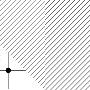
Figure 6. The spinor variety: drawing the matrix $\omega$, the vertical and horizontal lines through the lower left dot in the matrix contribute degree 1 line bundles to the normal bundle. The other unshaded stuff contributes degree 0.

9. Lagrangian–Grassmannian connections

For $G=\operatorname{Sp}\left({2n,\mathbb{C}}\right)$ the Maurer–Cartan 1-form is

$$\omega=\begin{pmatrix}\gamma&\xi\\ \eta&-{}^{t}{\gamma}\end{pmatrix}$$

where ${}^{t}{\eta}=\eta$ and ${}^{t}{\xi}=\xi$. The subalgebra $\mathfrak{p}$ given by $\omega=0$ is the Lie subalgebra of the subgroup $P$ preserving a Lagrangian $n$-plane, so $G/P$ is the Lagrangian–Grassmannian, $\operatorname{Lag}\left(\mathbb{C}^{2n}\right)$, i.e. the space of Lagrangian $n$-planes in $\mathbb{C}^{2n}$. Thus $\dim\operatorname{Lag}\left(\mathbb{C}^{2n}\right)=\frac{n(n+1)}{2}.$

Consider the circle subgroup given by setting all of the $\eta$ and $\xi$ components to $0$, except for one $\eta^{i}_{j}$ (which equals $\eta^{j}_{i}$) for some choice of $i\geq j$, the corresponding $\xi^{i}_{j}$, and $\gamma^{i}_{i}$ and $\gamma^{j}_{j}$, and finally impose the equation $\gamma^{j}_{j}=\gamma^{i}_{i}$. The circle subalgebra is isomorphic to $\mathfrak{sl}\left({2,\mathbb{C}}\right)$, and $\eta^{i}_{j}$ is semibasic, and therefore the orbit of this circle subgroup is a rational circle on the Lagrangian–Grassmannian.

The roots of $\operatorname{Sp}\left({2n,\mathbb{C}}\right)$ are $\pm\gamma^{i}_{i}\pm\gamma^{j}_{j}$ for $i\neq j$ and $\pm 2\gamma^{i}_{i}$. The roots omitted from $\mathfrak{p}$ are $\gamma^{i}_{i}+\gamma^{j}_{j}$ (where $i$ might equal $j$).

The components of $\eta$ on or under the diagonal (see Figure 7), on the same row or column as $\eta^{i}_{j}$, contribute $\mathcal{O}\left({1}\right)$ to the normal bundle, while all other $\eta$ components contribute $\mathcal{O}$, so $T(G/P)_{\mathbb{P}^{1}_{\alpha}}=\mathcal{O}\left({2}\right)\oplus\mathcal{O}^{\oplus{p_{0}}}\oplus\mathcal{O}\left({1}\right)^{\oplus{p_{1}}}$ with

$$p_{0}=\frac{n^{2}+n}{2}-p_{1},\quad p_{1}=n+i-j-1.$$

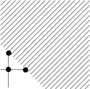
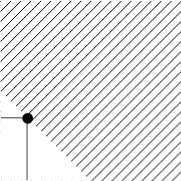
Figure 7. The Lagrangian–Grassmannian: (a) the vertical and horizontal lines through the lower left dot in the matrix contribute degree 1 line bundles to the normal bundle. (b) The count is slightly different when the root space lies on the diagonal.

10. Conclusions

Kobayashi invented invariant metrics for projective structures. For a generic Cartan geometry on a complex manifold, the circles of the model roll onto the manifold, but this rolling runs into singularities, rolling out not a rational curve but only a disk. The hyperbolic metrics on these disks are responsible for the Kobayashi metric on the manifold: define the distance between points to be the infimum distance measured along paths lying on finitely many of these disks, in their hyperbolic metrics.

On the other hand, the Cartan geometries attended to in the present article have quite degenerate Kobayashi metrics, at the opposite extreme. The next natural step is to investigate parabolic geometries which are just barely incomplete, for instance with all circles affine lines or elliptic curves. Such geometries might admit classification, although their analysis seems difficult in the absence of invariant metrics.

The approach of Jahnke & Radloff [24] should uncover the sporadic nature of curved parabolic geometries on smooth complex projective varieties. Roughly speaking, parabolic geometries appear to be rare, except perhaps on unspeakably complicated complex manifolds, and all known parabolic geometries on smooth projective varieties are flat. However, there are simple curved examples with singularities (see Hitchin [20] p. 83, example 3.3), which would appear to point the only way forward for research in parabolic geometry: curvature demands singularity.

References

- [1] Larry Bates, A symmetry completeness criterion for second-order differential equations, Proc. Amer. Math. Soc. 132 (2004), no. 6, 1785–1786 (electronic). MR MR2051142 (2005b:34076)
- [2] Robert A. Blumenthal, Cartan submersions and Cartan foliations, Illinois J. Math. 31 (1987), no. 2, 327–343. MR MR882118 (88f:53061)
- [3] Robert A. Blumenthal and James J. Hebda, The generalized Cartan-Ambrose-Hicks theorem, Geom. Dedicata 29 (1989), no. 2, 163–175. MR 90b:53035
- [4] Armand Borel, Linear algebraic groups, second ed., Graduate Texts in Mathematics, vol. 126, Springer-Verlag, New York, 1991. MR 92d:20001
- [5] by same author, Élie Cartan, Hermann Weyl et les connexions projectives, Essays on geometry and related topics, Vol. 1, 2, Monogr. Enseign. Math., vol. 38, Enseignement Math., Geneva, 2001, pp. 43–58. MR 2004a:53001
- [6] Andreas Čap, Two constructions with parabolic geometries, Proceedings of the 25th Winter School on Geometry and Physics, Srni 2005, 2005, math.DG/0504389, to appear in Rend. Circ. Mat. Palermo Suppl. ser. II, electronically available as ESI Preprint 1645, pp. 1–27.
- [7] Andreas Čap, Jan Slovák, and Vojtěch Žádník, On distinguished curves in parabolic geometries, Transform. Groups 9 (2004), no. 2, 143–166. MR MR2056534 (2005a:53042)
- [8] Élie Cartan, Les espaces à connexion conforme, Ann. Soc. Polon. Mat. 2 (1923), 171–221, Also in [13], pp. 747–797.
- [9] by same author, Sur les variétés à connection projective, Bull. Soc. Math. 52 (1924), 205–241.
- [10] by same author, Sur la géometrie pseudo–conforme des hypersurfaces de l’espace de deux variables complexes, I, Annali di Matematica Pura ed Applicata 11 (1932), 17–90, Also in [12], pp. 1232–1305.
- [11] by same author, Sur la géometrie pseudo–conforme des hypersurfaces de l’espace de deux variables complexes, II, Annali Sc. Norm. Sup. Pisa 1 (1932), 333–354, Also in [13], pp. 1217–1238.
- [12] by same author, Œuvres complètes. Partie II, second ed., Éditions du Centre National de la Recherche Scientifique (CNRS), Paris, 1984, Algèbre, systèmes différentiels et problèmes d’équivalence. [Algebra, differential systems and problems of equivalence]. MR 85g:01032b
- [13] by same author, Œuvres complètes. Partie III. Vol. 2, second ed., Éditions du Centre National de la Recherche Scientifique (CNRS), Paris, 1984, Géométrie différentielle. Divers. [Differential geometry. Miscellanea], With biographical material by Shiing Shen Chern, Claude Chevalley and J. H. C. Whitehead. MR 85g:01032d
- [14] Yeaton H. Clifton, On the completeness of Cartan connections, J. Math. Mech. 16 (1966), 569–576. MR MR0205183 (34 #5017)
- [15] Charles Ehresmann, Sur la notion d’espace complet en géométrie différentielle, C. R. Acad. Sci. Paris 202 (1936), 2033.
- [16] by same author, Sur les arcs analytique d’un espace de Cartan, C. R. Acad. Sci. Paris (1938), 1433.
- [17] by same author, Les connexions infinitésimales dans un espace fibré différentiable, Colloque de topologie (espaces fibrés), Bruxelles, 1950, Georges Thone, Liège, 1951, pp. 29–55. MR MR0042768 (13,159e)
- [18] William Fulton and Joe Harris, Representation theory, Graduate Texts in Mathematics, vol. 129, Springer-Verlag, New York, 1991, A first course, Readings in Mathematics. MR 93a:20069
- [19] R. C. Gunning, On uniformization of complex manifolds: the role of connections, Mathematical Notes, vol. 22, Princeton University Press, Princeton, N.J., 1978. MR 82e:32034
- [20] N. J. Hitchin, Complex manifolds and Einstein’s equations, Twistor geometry and nonlinear systems (Primorsko, 1980), Lecture Notes in Math., vol. 970, Springer, Berlin, 1982, pp. 73–99. MR 84i:32041
- [21] Jun-Muk Hwang and Ngaiming Mok, Uniruled projective manifolds with irreducible reductive -structures, J. Reine Angew. Math. 490 (1997), 55–64. MR MR1468924 (99h:32034)
- [22] Priska Jahnke and Ivo Radloff, Splitting jet sequences, Math. Res. Letters 11 (2004), 345–354, math.AG/0210454.
- [23] by same author, Threefolds with holomorphic normal projective connections, Math. Ann. 329 (2004), no. 3, 379–400, math.AG/0210117.
- [24] by same author, Projective threefolds with holomorphic conformal structure, Internat. J. Math. 16 (2005), no. 6, 595–607. MR MR2153485 (2006c:14062)
- [25] Shôshichi Kobayashi, Espaces à connexion de Cartan complets, Proc. Japan Acad. 30 (1954), 709–710. MR MR0069570 (16,1053d)
- [26] by same author, Transformation groups in differential geometry, Springer-Verlag, Berlin, 1995, Reprint of the 1972 edition. MR 96c:53040
- [27] Shôshichi Kobayashi and Tadashi Nagano, On projective connections, J. Math. Mech. 13 (1964), 215–235. MR 28 #2501
- [28] Claude LeBrun and L. J. Mason, Zoll manifolds and complex surfaces, J. Differential Geom. 61 (2002), no. 3, 453–535. MR 2004d:53043
- [29] William S. Massey, Algebraic topology: An introduction, Harcourt, Brace & World, Inc., New York, 1967. MR 35 #2271
- [30] Benjamin McKay, Complete projective connections, math.DG/0504082, April 2005.
- [31] by same author, Rational curves and parabolic geometries, math.DG/0603276, March 2006.
- [32] Richard S. Palais, A global formulation of the Lie theory of transformation groups, Mem. Amer. Math. Soc. No. 22 (1957), iii+123. MR 22 #12162
- [33] Jean-Pierre Serre, Complex semisimple Lie algebras, Springer Monographs in Mathematics, Springer-Verlag, Berlin, 2001, Translated from the French by G. A. Jones, Reprint of the 1987 edition. MR 2001h:17001
- [34] Richard W. Sharpe, Differential geometry, Graduate Texts in Mathematics, vol. 166, Springer-Verlag, New York, 1997, Cartan’s generalization of Klein’s Erlangen program, With a foreword by S. S. Chern. MR 98m:53033
- [35] Hsien-Chung Wang, Closed manifolds with homogeneous complex structure, Amer. J. Math. 76 (1954), 1–32. MR 16,518a