Least Angle Regression

Abstract

The purpose of model selection algorithms such as All Subsets, Forward Selection and Backward Elimination is to choose a linear model on the basis of the same set of data to which the model will be applied. Typically we have available a large collection of possible covariates from which we hope to select a parsimonious set for the efficient prediction of a response variable. Least Angle Regression (LARS), a new model selection algorithm, is a useful and less greedy version of traditional forward selection methods. Three main properties are derived: (1) A simple modification of the LARS algorithm implements the Lasso, an attractive version of ordinary least squares that constrains the sum of the absolute regression coefficients; the LARS modification calculates all possible Lasso estimates for a given problem, using an order of magnitude less computer time than previous methods. (2) A different LARS modification efficiently implements Forward Stagewise linear regression, another promising new model selection method; this connection explains the similar numerical results previously observed for the Lasso and Stagewise, and helps us understand the properties of both methods, which are seen as constrained versions of the simpler LARS algorithm. (3) A simple approximation for the degrees of freedom of a LARS estimate is available, from which we derive a $C_{p}$ estimate of prediction error; this allows a principled choice among the range of possible LARS estimates. LARS and its variants are computationally efficient: the paper describes a publicly available algorithm that requires only the same order of magnitude of computational effort as ordinary least squares applied to the full set of covariates.

, [1]T1Supported in part by NSF Grant DMS-00-72360 and NIH Grant 8R01-EB002784. , [2]T2Supported in part by NSF Grant DMS-02-04162 and NIH Grant R01-EB0011988-08. [3]T3Supported in part by NSF Grant DMS-00-72661 and NIH Grant R01-EB001988-08. and [4]T4Supported in part by NSF Grant DMS-99-71405 and NIH Grant 2R01-CA72028.

keywordAMSAMS 2000 subject classification.

1 Introduction.

Automatic model-building algorithms are familiar, and sometimes notorious, in the linear model literature: Forward Selection, Backward Elimination, All Subsets regression and various combinations are used to automatically produce “good” linear models for predicting a response $y$ on the basis of some measured covariates $x_{1},x_{2},\ldots,x_{m}$. Goodness is often defined in terms of prediction accuracy, but parsimony is another important criterion: simpler models are preferred for the sake of scientific insight into the $x-y$ relationship. Two promising recent model-building algorithms, the Lasso and Forward Stagewise linear regression, will be discussed here, and motivated in terms of a computationally simpler method called Least Angle Regression.

Least Angle Regression (LARS) relates to the classic model-selection method known as Forward Selection, or “forward stepwise regression,” described in Weisberg [(1980), Section 8.5]: given a collection of possible predictors, we select the one having largest absolute correlation with the response $y$, say $x_{j_{1}}$, and perform simple linear regression of $y$ on $x_{j_{1}}$. This leaves a residual vector orthogonal to $x_{j_{1}}$, now considered to be the response. We project the other predictors orthogonally to $x_{j_{1}}$ and repeat the selection process. After $k$ steps this results in a set of predictors $x_{j_{1}},x_{j_{2}},\ldots,x_{j_{k}}$ that are then used in the usual way to construct a $k$-parameter linear model. Forward Selection is an aggressive fitting technique that can be overly greedy, perhaps eliminating at the second step useful predictors that happen to be correlated with $x_{j_{1}}$.

Forward Stagewise, as described below, is a much more cautious version of Forward Selection, which may take thousands of tiny steps as it moves toward a final model. It turns out, and this was the original motivation for the LARS algorithm, that a simple formula allows Forward Stagewise to be implemented using fairly large steps, though not as large as a classic Forward Selection, greatly reducing the computational burden. The geometry of the algorithm, described in Section 2, suggests the name “Least Angle Regression.” It then happens that this same geometry applies to another, seemingly quite different, selection method called the Lasso [Tibshirani (1996)]. The LARS–Lasso–Stagewise connection is conceptually as well as computationally useful. The Lasso is described next, in terms of the main example used in this paper.

Table 1 shows a small part of the data for our main example.

Table 1: Diabetes study: $442$ diabetes patients were measured on $10$ baseline variables; a prediction model was desired for the response variable, a measure of disease progression one year after baseline

	AGE	SEX	BMI	BP	Serum measurements						Response
Patient	${\bf x_{1}}$	${\bf x_{2}}$	${\bf x_{3}}$	${\bf x_{4}}$	${\bf x_{5}}$	${\bf x_{6}}$	${\bf x_{7}}$	${\bf x_{8}}$	${\bf x_{9}}$	${\bf x_{10}}$	y
001	59	2	32.1	101	157	93.2	38	4	4.9	87	151
002	48	1	21.6	87	183	103.2	70	3	3.9	69	75
003	72	2	30.5	93	156	93.6	41	4	4.7	85	141
004	24	1	25.3	84	198	131.4	40	5	4.9	89	206
005	50	1	23.0	101	192	125.4	52	4	4.3	80	135
006	23	1	22.6	89	139	64.8	61	2	4.2	68	97
00 ⋮	⋮	⋮	⋮	⋮	⋮	⋮	⋮	⋮	⋮	⋮	⋮
441	36	1	30.0	95	201	125.2	42	5	5.1	85	220
442	36	1	19.6	71	250	133.2	97	3	4.6	92	57

Ten baseline variables, age, sex, body mass index, average blood pressure and six blood serum measurements, were obtained for each of $n=442$ diabetes patients, as well as the response of interest, a quantitative measure of disease progression one year after baseline. The statisticians were asked to construct a model that predicted response $y$ from covariates $x_{1},x_{2},\ldots,x_{10}$. Two hopes were evident here, that the model would produce accurate baseline predictions of response for future patients and that the form of the model would suggest which covariates were important factors in disease progression.

The Lasso is a constrained version of ordinary least squares (OLS). Let ${\bf x}_{1},{\bf x}_{2},\allowbreak\ldots,{\bf x}_{m}$ be $n$-vectors representing the covariates, $m=10$ and $n=442$ in the diabetes study, and let ${\bf y}$ be the vector of responses for the $n$ cases. By location and scale transformations we can always assume that the covariates have been standardized to have mean 0 and unit length, and that the response has mean 0,

$$\quad\sum_{i=1}^{n}y_{i}=0,\qquad\sum_{i=1}^{n}x_{ij}=0,\qquad\sum_{i=1}^{n}x_{ij}^{2}=1\qquad\mbox{for }j=1,2,\ldots,m.$$ (1)

This is assumed to be the case in the theory which follows, except that numerical results are expressed in the original units of the diabetes example.

A candidate vector of regression coefficients $\widehat{\bolds}{\beta}=(\widehat{\beta}_{1},\widehat{\beta}_{2},\ldots,\widehat{\beta}_{m})^{\prime}$ gives prediction vector $\widehat{\bolds{\mu}}$,

$$\widehat{\bolds{\mu}}=\sum_{j=1}^{m}{\bf x}_{j}\widehat{\beta}_{j}=X\widehat{\bolds}{\beta}\qquad[X_{n\times m}=({\bf x}_{1},{\bf x}_{2},\ldots,{\bf x}_{m})]$$ (2)

with total squared error

$$S(\widehat{\bolds}{\beta})=\|{\bf y}-\widehat{\bolds{\mu}}\|^{2}=\sum_{i=1}^{n}(y_{i}-\widehat{\mu}_{i})^{2}.$$ (3)

Let $T(\widehat{\bolds}{\beta})$ be the absolute norm of $\widehat{\bolds}{\beta}$,

$$T(\widehat{\bolds}{\beta})=\sum_{j=1}^{m}|\widehat{\beta}_{j}|.$$ (4)

The Lasso chooses $\widehat{\bolds}{\beta}$ by minimizing $S(\widehat{\bolds}{\beta})$ subject to a bound $t$ on $T(\widehat{\bolds}{\beta})$,

$$\mbox{{\it Lasso}:}\quad\mbox{minimize}\quad S(\widehat{\bolds}{\beta})\qquad\mbox{subject to}\quad T(\widehat{\bolds}{\beta})\leq t.$$ (5)

Quadratic programming techniques can be used to solve (5) though we will present an easier method here, closely related to the “homotopy method” of Osborne, Presnell and Turlach (2000a).

The left panel of Figure 1 shows all Lasso solutions $\widehat{\bolds}{\beta}(t)$ for the diabetes study, as $t$ increases from 0, where $\widehat{\bolds}{\beta}=0$, to $t=3460.00$, where $\widehat{\bolds}{\beta}$ equals the OLS regression vector, the constraint in (5) no longer binding. We see that the Lasso tends to shrink the OLS coefficients toward 0, more so for small values of $t$. Shrinkage often improves prediction accuracy, trading off decreased variance for increased bias as discussed in Hastie, Tibshirani and Friedman (2001).

The Lasso also has a parsimony property: for any given constraint value $t$, only a subset of the covariates have nonzero values of $\widehat{\beta}_{j}$. At $t=1000$, for example, only variables 3, 9, 4 and 7 enter the Lasso regression model (2). If this model provides adequate predictions, a crucial question considered in Section 4, the statisticians could report these four variables as the important ones.

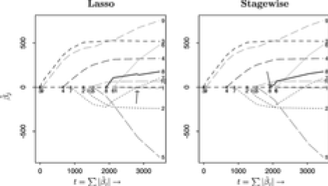
Figure 1: Estimates of regression coefficients $\widehat{\beta}_{j}$, $j=1,2,\ldots,10$, for the diabetes study. (Left panel) Lasso estimates, as a function of $t=\sum_{j}|\widehat{\beta}_{j}|$. The covariates enter the regression equation sequentially as $t$ increases, in order $j=3,9,4,7,\ldots,1$. (Right panel) The same plot for Forward Stagewise Linear Regression. The two plots are nearly identical, but differ slightly for large $t$ as shown in the track of covariate $8$.

Forward Stagewise Linear Regression, henceforth called Stagewise, is an iterative technique that begins with $\widehat{\bolds{\mu}}=0$ and builds up the regression function in successive small steps. If $\widehat{\bolds{\mu}}$ is the current Stagewise estimate, let ${\bf c}(\widehat{\bolds{\mu}})$ be the vector of current correlations

$$\widehat{\bf c}={\bf c}(\widehat{\bolds{\mu}})=X^{\prime}({\bf y}-\widehat{\bolds{\mu}}),$$ (6)

so that $\widehat{c}_{j}$ is proportional to the correlation between covariate $x_{j}$ and the current residual vector. The next step of the Stagewise algorithm is taken in the direction of the greatest current correlation,

$$\widehat{j}=\arg\max|\widehat{c}_{j}|\quad\mbox{and}\quad\widehat{\bolds{\mu}}\rightarrow\widehat{\bolds{\mu}}+\varepsilon\cdot\operatorname{sign}(\widehat{c}_{\hat{j}})\cdot{\bf x}_{\hat{j}},$$ (7)

with $\varepsilon$ some small constant. “Small” is important here: the “big” choice $\varepsilon=|\widehat{c}_{\hat{j}}|$ leads to the classic Forward Selection technique, which can be overly greedy, impulsively eliminating covariates which are correlated with $x_{\hat{j}}$. The Stagewise procedure is related to boosting and also to Friedman’s MART algorithm [Friedman (2001)]; see Section 8, as well as Hastie, Tibshirani and Friedman [(2001), Chapter 10 and Algorithm 10.4].

The right panel of Figure 1 shows the coefficient plot for Stagewise applied to the diabetes data. The estimates were built up in 6000 Stagewise steps [making $\varepsilon$ in (7) small enough to conceal the “Etch-a-Sketch” staircase seen in Figure 2, Section 2]. The striking fact is the similarity between the Lasso and Stagewise estimates. Although their definitions look completely different, the results are nearly, but not exactly, identical.

The main point of this paper is that both Lasso and Stagewise are variants of a basic procedure called Least Angle Regression, abbreviated LARS (the “S” suggesting “Lasso” and “Stagewise”). Section 2 describes the LARS algorithm while Section 3 discusses modifications that turn LARS into Lasso or Stagewise, reducing the computational burden by at least an order of magnitude for either one. Sections 5 and 6 verify the connections stated in Section 3.

Least Angle Regression is interesting in its own right, its simple structure lending itself to inferential analysis. Section 4 analyzes the “degrees of freedom” of a LARS regression estimate. This leads to a $C_{p}$ type statistic that suggests which estimate we should prefer among a collection of possibilities like those in Figure 1. A particularly simple $C_{p}$ approximation, requiring no additional computation beyond that for the $\widehat{\bolds}{\beta}$ vectors, is available for LARS.

Section 7 briefly discusses computational questions. An efficient $S$ program for all three methods, LARS, Lasso and Stagewise, is available. Section 8 elaborates on the connections with boosting.

2 The LARS algorithm.

Least Angle Regression is a stylized version of the Stagewise procedure that uses a simple mathematical formula to accelerate the computations. Only $m$ steps are required for the full set of solutions, where $m$ is the number of covariates: $m=10$ in the diabetes example compared to the 6000 steps used in the right panel of Figure 1. This section describes the LARS algorithm. Modifications of LARS that produce Lasso and Stagewise solutions are discussed in Section 3, and verified in Sections 5 and 6. Section 4 uses the simple structure of LARS to help analyze its estimation properties.

The LARS procedure works roughly as follows. As with classic Forward Selection, we start with all coefficients equal to zero, and find the predictor most correlated with the response, say $x_{j_{1}}$. We take the largest step possible in the direction of this predictor until some other predictor, say $x_{j_{2}}$, has as much correlation with the current residual. At this point LARS parts company with Forward Selection. Instead of continuing along $x_{j_{1}}$, LARS proceeds in a direction equiangular between the two predictors until a third variable $x_{j_{3}}$ earns its way into the “most correlated” set. LARS then proceeds equiangularly between $x_{j_{1}},x_{j_{2}}$ and $x_{j_{3}}$, that is, along the “least angle direction,” until a fourth variable enters, and so on.

The remainder of this section describes the algebra necessary to execute the equiangular strategy. As usual the algebraic details look more complicated than the simple underlying geometry, but they lead to the highly efficient computational algorithm described in Section 7.

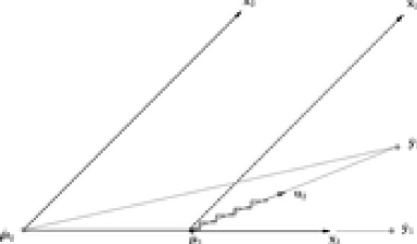
Figure 2: The LARS algorithm in the case of $m=2$ covariates; $\bar{\bf y}_{2}$ is the projection of ${\bf y}$ into ${\mathcal{L}}({\bf x}_{1},{\bf x}_{2})$. Beginning at $\widehat{\bolds{\mu}}_{0}={\bf 0}$, the residual vector $\bar{\bf y}_{2}-\widehat{\bolds{\mu}}_{0}$ has greater correlation with ${\bf x}_{1}$ than ${\bf x}_{2}$; the next LARS estimate is $\widehat{\bolds{\mu}}_{1}=\widehat{\bolds{\mu}}_{0}+\widehat{\gamma}_{1}{\bf x}_{1}$, where $\widehat{\gamma}_{1}$ is chosen such that $\bar{\bf y}_{2}-\widehat{\bolds{\mu}}_{1}$ bisects the angle between ${\bf x}_{1}$ and ${\bf x}_{2}$; then $\widehat{\bolds{\mu}}_{2}=\widehat{\bolds{\mu}}_{1}+\widehat{\gamma}_{2}{\bf u}_{2}$, where ${\bf u}_{2}$ is the unit bisector; $\widehat{\bolds{\mu}}_{2}=\bar{\bf y}_{2}$ in the case $m=2$, but not for the case $m>2$; see Figure 4. The staircase indicates a typical Stagewise path. Here LARS gives the Stagewise track as $\varepsilon\rightarrow 0$, but a modification is necessary to guarantee agreement in higher dimensions; see Section 3.2.

LARS builds up estimates $\widehat{\bolds{\mu}}=X\widehat{\bolds}{\beta}$, (2), in successive steps, each step adding one covariate to the model, so that after $k$ steps just $k$ of the $\widehat{\beta}_{j}$’s are nonzero. Figure 2 illustrates the algorithm in the situation with $m=2$ covariates, $X=({\bf x}_{1},{\bf x}_{2})$. In this case the current correlations (6) depend only on the projection $\bar{\bf y}_{2}$ of ${\bf y}$ into the linear space ${\mathcal{L}}(X)$ spanned by ${\bf x}_{1}$ and ${\bf x}_{2}$,

$${\bf c}(\widehat{\bolds{\mu}})=X^{\prime}({\bf y}-\widehat{\bolds{\mu}})=X^{\prime}(\bar{\bf y}_{2}-\widehat{\bolds{\mu}}).$$ (8)

The algorithm begins at $\widehat{\bolds{\mu}}_{0}={\bf 0}$ [remembering that the response has had its mean subtracted off, as in (1)]. Figure 2 has $\bar{\bf y}_{2}-\widehat{\bolds{\mu}}_{0}$ making a smaller angle with ${\bf x}_{1}$ than ${\bf x}_{2}$, that is, $c_{1}(\widehat{\bolds{\mu}}_{0})>c_{2}(\widehat{\bolds{\mu}}_{0})$. LARS then augments $\widehat{\bolds{\mu}}_{0}$ in the direction of ${\bf x}_{1}$, to

$$\widehat{\bolds{\mu}}_{1}=\widehat{\bolds{\mu}}_{0}+\widehat{\gamma}_{1}{\bf x}_{1}.$$ (9)

Stagewise would choose $\widehat{\gamma}_{1}$ equal to some small value $\varepsilon$, and then repeat the process many times. Classic Forward Selection would take $\widehat{\gamma}_{1}$ large enough to make $\widehat{\bolds{\mu}}_{1}$ equal $\bar{\bf y}_{1}$, the projection of ${\bf y}$ into ${\mathcal{L}}({\bf x}_{1})$. LARS uses an intermediate value of $\widehat{\gamma}_{1}$, the value that makes $\bar{\bf y}_{2}-\widehat{\bolds{\mu}}$, equally correlated with ${\bf x}_{1}$ and ${\bf x}_{2}$; that is, $\bar{\bf y}_{2}-\widehat{\bolds{\mu}}_{1}$ bisects the angle between ${\bf x}_{1}$ and ${\bf x}_{2}$, so $c_{1}(\widehat{\bolds{\mu}}_{1})=c_{2}(\widehat{\bolds{\mu}}_{1})$.

Let ${\bf u}_{2}$ be the unit vector lying along the bisector. The next LARS estimate is

$$\widehat{\bolds{\mu}}_{2}=\widehat{\bolds{\mu}}_{1}+\widehat{\gamma}_{2}{\bf u}_{2},$$ (10)

with $\widehat{\gamma}_{2}$ chosen to make $\widehat{\bolds{\mu}}_{2}=\bar{\bf y}_{2}$ in the case $m=2$. With $m>2$ covariates, $\widehat{\gamma}_{2}$ would be smaller, leading to another change of direction, as illustrated in Figure 4. The “staircase” in Figure 2 indicates a typical Stagewise path. LARS is motivated by the fact that it is easy to calculate the step sizes $\widehat{\gamma}_{1},\widehat{\gamma}_{2},\ldots$ theoretically, short-circuiting the small Stagewise steps.

Subsequent LARS steps, beyond two covariates, are taken along equiangular vectors, generalizing the bisector ${\bf u}_{2}$ in Figure 2. We assume that the covariate vectors ${\bf x}_{1},{\bf x}_{2},\ldots,{\bf x}_{m}$ are linearly independent. For ${\mathcal{A}}$ a subset of the indices $\{1,2,\ldots,m\}$, define the matrix

$$X_{\mathcal{A}}=(\cdots\,s_{j}{\bf x}_{j}\,\cdots)_{j\in{\mathcal{A}}},$$ (11)

where the signs $s_{j}$ equal $\pm 1$. Let

$${\mathcal{G}}_{\mathcal{A}}=X_{\mathcal{A}}^{\prime}X_{\mathcal{A}}\quad\mbox{and}\quad A_{\mathcal{A}}=(\bolds{1}_{\mathcal{A}}^{\prime}{\mathcal{G}}_{\mathcal{A}}^{-1}\bolds{1}_{\mathcal{A}})^{-1/2},$$ (12)

$\bolds{1}_{\mathcal{A}}$ being a vector of 1’s of length equaling $|\mathcal{A}|$, the size of ${\mathcal{A}}$. The

$$\mbox{\it equiangular vector}\quad{\bf u}_{\mathcal{A}}=X_{\mathcal{A}}w_{\mathcal{A}}\qquad\mbox{where }w_{\mathcal{A}}=A_{\mathcal{A}}G_{\mathcal{A}}^{-1}\bolds{1}_{\mathcal{A}},$$ (13)

is the unit vector making equal angles, less than $90^{\circ}$, with the columns of $X_{\mathcal{A}}$,

$$X_{\mathcal{A}}^{\prime}{\bf u}_{\mathcal{A}}=A_{\mathcal{A}}\bolds{1}_{\mathcal{A}}\quad\mbox{and}\quad\|{\bf u}_{\mathcal{A}}\|^{2}=1.$$ (14)

We can now fully describe the LARS algorithm. As with the Stagewise procedure we begin at $\widehat{\bolds{\mu}}_{0}={\bf 0}$ and build up $\widehat{\bolds{\mu}}$ by steps, larger steps in the LARS case. Suppose that $\widehat{\bolds{\mu}}_{\mathcal{A}}$ is the current LARS estimate and that

$$\widehat{\bf c}=X^{\prime}({\bf y}-\widehat{\bolds{\mu}}_{\mathcal{A}})$$ (15)

is the vector of current correlations (6). The active set ${\mathcal{A}}$ is the set of indices corresponding to covariates with the greatest absolute current correlations,

$$\widehat{C}=\max_{j}\{|\widehat{c}_{j}|\}\quad\mbox{and}\quad{\mathcal{A}}=\{j\dvtx|\widehat{c}_{j}|=\widehat{C}\}.$$ (16)

Letting

$$s_{j}=\operatorname{sign}\{\widehat{c}_{j}\}\qquad\mbox{for }j\in{\mathcal{A}},$$ (17)

we compute $X_{\mathcal{A}},A_{\mathcal{A}}$ and ${\bf u}_{\mathcal{A}}$ as in (11)–(13), and also the inner product vector

$${\bf a}\equiv X^{\prime}{\bf u}_{\mathcal{A}}.$$ (18)

Then the next step of the LARS algorithm updates $\widehat{\bolds{\mu}}_{\mathcal{A}}$, say to

$$\widehat{\bolds{\mu}}_{{\mathcal{A}}_{+}}=\widehat{\bolds{\mu}}_{\mathcal{A}}+\widehat{\gamma}{\bf u}_{\mathcal{A}},$$ (19)

where

$$\widehat{\gamma}=\min_{j\in{\mathcal{A}}^{c}}{}^{\!\!+}\biggl{\{}\frac{\widehat{C}-\widehat{c}_{j}}{A_{\mathcal{A}}-a_{j}},\frac{\widehat{C}+\widehat{c}_{j}}{A_{\mathcal{A}}+a_{j}}\biggr{\}};$$ (20)

“$\min^{+}$” indicates that the minimum is taken over only positive components within each choice of $j$ in (20).

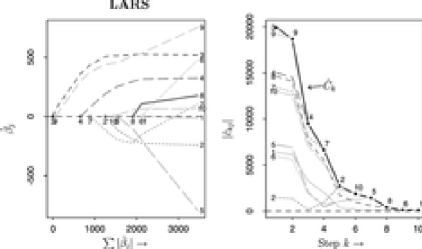
Figure 3: LARS analysis of the diabetes study: (left) estimates of regression coefficients $\widehat{\beta}_{j}$, $j=1,2,\ldots,10$; plotted versus $\sum|\widehat{\beta}_{j}|$; plot is slightly different than either Lasso or Stagewise, Figure 1; (right) absolute current correlations as function of LARS step; variables enter active set $(\ref{eqn2.9})$ in order $3,9,4,7,\ldots,1$; heavy curve shows maximum current correlation $\widehat{C}_{k}$ declining with $k$.

Formulas (19) and (20) have the following interpretation: define

$${\bolds{\mu}}(\gamma)=\widehat{\bolds{\mu}}_{\mathcal{A}}+\gamma{\bf u}_{\mathcal{A}},$$ (21)

for $\gamma>0$, so that the current correlation

$$c_{j}(\gamma)={\bf x}_{j}^{\prime}\bigl{(}{\bf y}-{\bolds{\mu}}(\gamma)\bigr{)}=\widehat{c}_{j}-\gamma a_{j}.$$ (22)

For $j\in{\mathcal{A}}$, (14)–(16) yield

$$|c_{j}(\gamma)|=\widehat{C}-\gamma A_{\mathcal{A}},$$ (23)

showing that all of the maximal absolute current correlations decline equally. For $j\in{\mathcal{A}}^{c}$, equating (22) with (23) shows that $c_{j}(\gamma)$ equals the maximal value at $\gamma=(\widehat{C}-\widehat{c}_{j})/(A_{\mathcal{A}}-a_{j})$. Likewise $-c_{j}(\gamma)$, the current correlation for the reversed covariate $-{\bf x}_{j}$, achieves maximality at $(\widehat{C}+\widehat{c}_{j})/(A_{\mathcal{A}}+a_{j})$. Therefore $\widehat{\gamma}$ in (20) is the smallest positive value of $\gamma$ such that some new index $\widehat{j}$ joins the active set; $\widehat{j}$ is the minimizing index in (20), and the new active set ${\mathcal{A}}_{+}$ is ${\mathcal{A}}\cup\{\widehat{j}\}$; the new maximum absolute correlation is $\widehat{C}_{+}=\widehat{C}-\widehat{\gamma}A_{\mathcal{A}}$.

Figure 3 concerns the LARS analysis of the diabetes data. The complete algorithm required only $m=10$ steps of procedure (15)–(20), with the variables joining the active set ${\mathcal{A}}$ in the same order as for the Lasso: $3,9,4,7,\ldots,1$. Tracks of the regression coefficients $\widehat{\beta}_{j}$ are nearly but not exactly the same as either the Lasso or Stagewise tracks of Figure 1.

The right panel shows the absolute current correlations

$$|\widehat{c}_{kj}|=|{\bf x}_{j}^{\prime}({\bf y}-\widehat{\bolds{\mu}}_{k-1})|$$ (24)

for variables $j=1,2,\ldots,10$, as a function of the LARS step $k$. The maximum correlation

$$\widehat{C}_{k}=\max\{|\widehat{c}_{kj}|\}=\widehat{C}_{k-1}-\widehat{\gamma}_{k-1}A_{k-1}$$ (25)

declines with $k$, as it must. At each step a new variable $j$ joins the active set, henceforth having $|\widehat{c}_{kj}|=\widehat{C}_{k}$. The sign $s_{j}$ of each ${\bf x}_{j}$ in (11) stays constant as the active set increases.

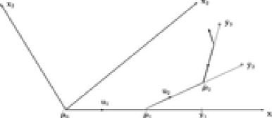
Figure 4: At each stage the LARS estimate $\widehat{\bolds{\mu}}_{k}$ approaches, but does not reach, the corresponding OLS estimate $\bar{\bf y}_{k}$.

Section 4 makes use of the relationship between Least Angle Regression and Ordinary Least Squares illustrated in Figure 4. Suppose LARS has just completed step $k-1$, giving $\widehat{\bolds{\mu}}_{k-1}$, and is embarking upon step $k$. The active set ${\mathcal{A}}_{k}$, (16), will have $k$ members, giving $X_{k},{\mathcal{G}}_{k},A_{k}$ and ${\bf u}_{k}$ as in (11)–(13) (here replacing subscript ${\mathcal{A}}$ with “$k$”). Let $\bar{\bf y}_{k}$ indicate the projection of ${\bf y}$ into ${\mathcal{L}}(X_{k})$, which, since $\widehat{\bolds{\mu}}_{k-1}\in{\mathcal{L}}(X_{k-1})$, is

$$\bar{\bf y}_{k}=\widehat{\bolds{\mu}}_{k-1}+X_{k}{\mathcal{G}}_{k}^{-1}X_{k}^{\prime}({\bf y}-\widehat{\bolds{\mu}}_{k-1})=\widehat{\bolds{\mu}}_{k-1}+\frac{\widehat{C}_{k}}{A_{k}}\ {\bf u}_{k},$$ (26)

the last equality following from (13) and the fact that the signed current correlations in ${\mathcal{A}}_{k}$ all equal $\widehat{C}_{k}$,

$$X_{k}^{\prime}({\bf y}-\widehat{\bolds{\mu}}_{k-1})=\widehat{C}_{k}\bolds{1}_{\mathcal{A}}.$$ (27)

Since ${\bf u}_{k}$ is a unit vector, (26) says that $\bar{\bf y}_{k}-\widehat{\bolds{\mu}}_{k-1}$ has length

$$\bar{\gamma}_{k}\equiv\frac{\widehat{C}_{k}}{A_{k}}.$$ (28)

Comparison with (19) shows that the LARS estimate $\widehat{\bolds{\mu}}_{k}$ lies on the line from $\widehat{\bolds{\mu}}_{k-1}$ to $\bar{\bf y}_{k}$,

$$\widehat{\bolds{\mu}}_{k}-\widehat{\bolds{\mu}}_{k-1}=\frac{\widehat{\gamma}_{k}}{\bar{\gamma}_{k}}\ (\bar{\bf y}_{k}-\widehat{\bolds{\mu}}_{k-1}).$$ (29)

It is easy to see that $\widehat{\gamma}_{k}$, (19), is always less than $\bar{\gamma}_{k}$, so that $\widehat{\bolds{\mu}}_{k}$ lies closer than $\bar{\bf y}_{k}$ to $\widehat{\bolds{\mu}}_{k-1}$. Figure 4 shows the successive LARS estimates $\widehat{\bolds{\mu}}_{k}$ always approaching but never reaching the OLS estimates $\bar{\bf y}_{k}$.

The exception is at the last stage: since ${\mathcal{A}}_{m}$ contains all covariates, (20) is not defined. By convention the algorithm takes $\widehat{\gamma}_{m}=\bar{\gamma}_{m}=\widehat{C}_{m}/A_{m}$, making $\widehat{\bolds{\mu}}_{m}=\bar{\bf y}_{m}$ and $\widehat{\bolds}{\beta}_{m}$ equal the OLS estimate for the full set of $m$ covariates.

The LARS algorithm is computationally thrifty. Organizing the calculations correctly, the computational cost for the entire $m$ steps is of the same order as that required for the usual Least Squares solution for the full set of $m$ covariates. Section 7 describes an efficient LARS program available from the authors. With the modifications described in the next section, this program also provides economical Lasso and Stagewise solutions.

3 Modified versions of Least Angle Regression.

Figures 1 and 3 show Lasso, Stagewise and LARS yielding remarkably similar estimates for the diabetes data. The similarity is no coincidence. This section describes simple modifications of the LARS algorithm that produce Lasso or Stagewise estimates. Besides improved computational efficiency, these relationships elucidate the methods’ rationale: all three algorithms can be viewed as moderately greedy forward stepwise procedures whose forward progress is determined by compromise among the currently most correlated covariates. LARS moves along the most obvious compromise direction, the equiangular vector (13), while Lasso and Stagewise put some restrictions on the equiangular strategy.

3.1 The LARS–Lasso relationship.

The full set of Lasso solutions, as shown for the diabetes study in Figure 1, can be generated by a minor modification of the LARS algorithm (15)–(20). Our main result is described here and verified in Section 5. It closely parallels the homotopy method in the papers by Osborne, Presnell and Turlach (2000a, b), though the LARS approach is somewhat more direct.

Let $\widehat{\bolds}{\beta}$ be a Lasso solution (5), with $\widehat{\bolds{\mu}}=X\widehat{\bolds}{\beta}$. Then it is easy to show that the sign of any nonzero coordinate $\widehat{\beta}_{j}$ must agree with the sign $s_{j}$ of the current correlation $\widehat{c}_{j}={\bf x}_{j}^{\prime}({\bf y}-\widehat{\bolds{\mu}})$,

$$\operatorname{sign}(\widehat{\beta}_{j})=\operatorname{sign}(\,\widehat{c}_{j})=s_{j};$$ (30)

see Lemma 5.5 of Section 5. The LARS algorithm does not enforce restriction (30), but it can easily be modified to do so.

Suppose we have just completed a LARS step, giving a new active set ${\mathcal{A}}$ as in (16), and that the corresponding LARS estimate $\widehat{\bolds{\mu}}_{\mathcal{A}}$ corresponds to a Lasso solution $\widehat{\bolds{\mu}}=X\widehat{\bolds}{\beta}$. Let

$$w_{\mathcal{A}}=A_{\mathcal{A}}{\mathcal{G}}_{\mathcal{A}}^{-1}\bolds{1}_{\mathcal{A}},$$ (31)

a vector of length the size of ${\mathcal{A}}$, and (somewhat abusing subscript notation) define $\widehat{\bf d}$ to be the $m$-vector equaling $s_{j}w_{{\mathcal{A}}j}$ for $j\in{\mathcal{A}}$ and zero elsewhere. Moving in the positive $\gamma$ direction along the LARS line (21), we see that

$${\bolds{\mu}}(\gamma)=X\bolds{\beta}(\gamma),\qquad\mbox{where }\beta_{j}(\gamma)=\widehat{\beta}_{j}+\gamma\widehat{d}_{j}$$ (32)

for $j\in{\mathcal{A}}$. Therefore $\beta_{j}(\gamma)$ will change sign at

$$\gamma_{j}=-\widehat{\beta}_{j}/\widehat{d}_{j},$$ (33)

the first such change occurring at

$$\widetilde{\gamma}=\min_{\gamma_{j}>0}\{\gamma_{j}\},$$ (34)

say for covariate $x_{\tilde{j}}$; $\widetilde{\gamma}$ equals infinity by definition if there is no $\gamma_{j}>0$.

If $\widetilde{\gamma}$ is less than $\widehat{\gamma}$, (20), then $\beta_{j}(\gamma)$ cannot be a Lasso solution for $\gamma>\widetilde{\gamma}$ since the sign restriction (30) must be violated: $\beta_{\tilde{j}}(\gamma)$ has changed sign while $c_{\tilde{j}}(\gamma)$ has not. [The continuous function $c_{\tilde{j}}(\gamma)$ cannot change sign within a single LARS step since $|c_{\tilde{j}}(\gamma)|=\widehat{C}-\gamma A_{\mathcal{A}}>0$, (23).]

If $\widetilde{\gamma}<\widehat{\gamma}$, stop the ongoing LARS step at $\gamma=\widetilde{\gamma}$ and remove $\widetilde{j}$ from the calculation of the next equiangular direction. That is,

$$\widehat{\bolds{\mu}}_{{\mathcal{A}}_{+}}=\widehat{\bolds{\mu}}_{\mathcal{A}}+\widetilde{\gamma}{\bf u}_{\mathcal{A}}\quad\mbox{and}\quad{\mathcal{A}}_{+}={\mathcal{A}}-\{\widetilde{j}\}$$ (35)

rather than (19).

Theorem 1.

Under the Lasso modification, and assuming the “one at a time” condition discussed below, the LARS algorithm yields all Lasso solutions.

The active sets ${\mathcal{A}}$ grow monotonically larger as the original LARS algorithm progresses, but the Lasso modification allows ${\mathcal{A}}$ to decrease. “One at a time” means that the increases and decreases never involve more than a single index $j$. This is the usual case for quantitative data and can always be realized by adding a little jitter to the $y$ values. Section 5 discusses tied situations.

The Lasso diagram in Figure 1 was actually calculated using the modified LARS algorithm. Modification (35) came into play only once, at the arrowed point in the left panel. There ${\mathcal{A}}$ contained all 10 indices while ${\mathcal{A}}_{+}={\mathcal{A}}-\{7\}$. Variable 7 was restored to the active set one LARS step later, the next and last step then taking $\widehat{\bolds}{\beta}$ all the way to the full OLS solution. The brief absence of variable 7 had an effect on the tracks of the others, noticeably $\widehat{\beta}_{8}$. The price of using Lasso instead of unmodified LARS comes in the form of added steps, 12 instead of 10 in this example. For the more complicated “quadratic model” of Section 4, the comparison was 103 Lasso steps versus 64 for LARS.

3.2 The LARS–Stagewise relationship.

The staircase in Figure 2 indicates how the Stagewise algorithm might proceed forward from $\widehat{\bolds{\mu}}_{1}$, a point of equal current correlations $\widehat{c}_{1}=\widehat{c}_{2}$, (15). The first small step has (randomly) selected index $j=1$, taking us to $\widehat{\bolds{\mu}}_{1}+\varepsilon{\bf x}_{1}$. Now variable 2 is more correlated,

$${\bf x}_{2}^{\prime}({\bf y}-\widehat{\bolds{\mu}}_{1}-\varepsilon{\bf x}_{1})>{\bf x}_{1}^{\prime}({\bf y}-\widehat{\bolds{\mu}}_{1}-\varepsilon{\bf x}_{1}),$$ (36)

forcing $j=2$ to be the next Stagewise choice and so on.

We will consider an idealized Stagewise procedure in which the step size $\varepsilon$ goes to zero. This collapses the staircase along the direction of the bisector ${\bf u}_{2}$ in Figure 2, making the Stagewise and LARS estimates agree. They always agree for $m=2$ covariates, but another modification is necessary for LARS to produce Stagewise estimates in general. Section 6 verifies the main result described next.

Suppose that the Stagewise procedure has taken $N$ steps of infinitesimal size $\varepsilon$ from some previous estimate $\widehat{\bolds{\mu}}$, with

$$N_{j}\equiv\#\{\mbox{steps with selected index }j\},\qquad j=1,2,\ldots,m.$$ (37)

It is easy to show, as in Lemma 6.1 of Section 6, that $N_{j}=0$ for $j$ not in the active set ${\mathcal{A}}$ defined by the current correlations ${\bf x}_{j}^{\prime}({\bf y}-\widehat{\bolds{\mu}})$, (16). Letting

$$P\equiv(N_{1},N_{2},\ldots,N_{m})/N,$$ (38)

with $P_{\mathcal{A}}$ indicating the coordinates of $P$ for $j\in{\mathcal{A}}$, the new estimate is

$${\bolds{\mu}}=\widehat{\bolds{\mu}}+N\varepsilon X_{\mathcal{A}}P_{\mathcal{A}}\qquad[(\ref{eqn2.4})].$$ (39)

(Notice that the Stagewise steps are taken along the directions $s_{j}{\bf x}_{j}$.)

The LARS algorithm (21) progresses along

$${\bolds{\mu}}_{\mathcal{A}}+\gamma X_{\mathcal{A}}w_{\mathcal{A}},\qquad\mbox{where }w_{\mathcal{A}}=A_{\mathcal{A}}{\mathcal{G}}_{\mathcal{A}}^{-1}\bolds{1}_{\mathcal{A}}\qquad[(\ref{eqn2.6})\mbox{--}(\ref{eqn3.2})].$$ (40)

Comparing (39) with (40) shows that LARS cannot agree with Stagewise if $w_{\mathcal{A}}$ has negative components, since $P_{\mathcal{A}}$ is nonnegative. To put it another way, the direction of Stagewise progress $X_{\mathcal{A}}P_{\mathcal{A}}$ must lie in the convex cone generated by the columns of $X_{\mathcal{A}}$,

$${\mathcal{C}}_{\mathcal{A}}=\Biggl{\{}{\bf v}=\sum_{j\in{\mathcal{A}}}s_{j}{\bf x}_{j}P_{j},\ P_{j}\geq 0\Biggr{\}}.$$ (41)

If ${\bf u}_{\mathcal{A}}\in{\mathcal{C}}_{\mathcal{A}}$ then there is no contradiction between (41) and (42). If not it seems natural to replace ${\bf u}_{\mathcal{A}}$ with its projection into ${\mathcal{C}}_{\mathcal{A}}$, that is, the nearest point in the convex cone.

Proceed as in (15)–(20), except with ${\bf u}_{\mathcal{A}}$ replaced by ${\bf u}_{\hat{\mathcal{B}}}$, the unit vector lying along the projection of ${\bf u}_{\mathcal{A}}$ into ${\mathcal{C}}_{\mathcal{A}}$. (See Figure 9 in Section 6.)

Theorem 2.

Under the Stagewise modification, the LARS algorithm yields all Stagewise solutions.

The vector ${\bf u}_{\hat{\mathcal{B}}}$ in the Stagewise modification is the equiangular vector (13) for the subset $\widehat{\mathcal{B}}\subseteq{\mathcal{A}}$ corresponding to the face of ${\mathcal{C}}_{\mathcal{A}}$ into which the projection falls. Stagewise is a LARS type algorithm that allows the active set to decrease by one or more indices. This happened at the arrowed point in the right panel of Figure 1: there the set ${\mathcal{A}}=\{3,9,4,7,2,10,5,8\}$ was decreased to $\widehat{\mathcal{B}}={\mathcal{A}}-\{3,7\}$. It took a total of 13 modified LARS steps to reach the full OLS solution $\bar{\bolds{\beta}}_{m}=(X^{\prime}X)^{-1}X^{\prime}{\bf y}$. The three methods, LARS, Lasso and Stagewise, always reach OLS eventually, but LARS does so in only $m$ steps while Lasso and, especially, Stagewise can take longer. For the $m=64$ quadratic model of Section 4, Stagewise took 255 steps.

According to Theorem 2 the difference between successive Stagewise–modified LARS estimates is

$$\widehat{\bolds{\mu}}_{{\mathcal{A}}_{+}}-\widehat{\bolds{\mu}}_{\mathcal{A}}=\widehat{\gamma}{\bf u}_{\hat{\mathcal{B}}}=\widehat{\gamma}X_{\hat{\mathcal{B}}}w_{\hat{\mathcal{B}}},$$ (42)

as in (42). Since ${\bf u}_{\hat{\mathcal{B}}}$ exists in the convex cone ${\mathcal{C}}_{\mathcal{A}}$, $w_{\hat{\mathcal{B}}}$ must have nonnegative components. This says that the difference of successive coefficient estimates for coordinate $j\in{\widehat{\mathcal{B}}}$ satisfies

$$\operatorname{sign}(\widehat{\beta}_{+j}-\widehat{\beta}_{j})=s_{j},$$ (43)

where $s_{j}=\operatorname{sign}\{{\bf x}_{j}^{\prime}({\bf y}-\widehat{\bolds{\mu}})\}$.

We can now make a useful comparison of the three methods:

1. Stagewise—successive differences of $\widehat{\beta}_{j}$ agree in sign with the current correlation $\widehat{c}_{j}={\bf x}_{j}^{\prime}({\bf y}-\widehat{\bolds{\mu}})$;

2. Lasso—$\widehat{\beta}_{j}$ agrees in sign with $\widehat{c}_{j}$;

3. LARS—no sign restrictions (but see Lemma 5.1 of Section 5).

From this point of view, Lasso is intermediate between the LARS and Stagewise methods.

The successive difference property (43) makes the Stagewise $\widehat{\beta}_{j}$ estimates move monotonically away from 0. Reversals are possible only if $\widehat{c}_{j}$ changes sign while $\widehat{\beta}_{j}$ is “resting” between two periods of change. This happened to variable 7 in Figure 1 between the 8th and 10th Stagewise-modified LARS steps.

3.3 Simulation study.

A small simulation study was carried out comparing the LARS, Lasso and Stagewise algorithms. The $X$ matrix for the simulation was based on the diabetes example of Table 1, but now using a “Quadratic Model” having $m=64$ predictors, including interactions and squares of the 10 original covariates:

$$\mbox{\em Quadratic Model}\quad\mbox{10 main effects},45\mbox{ interactions},9\mbox{ squares},$$ (44)

the last being the squares of each ${\bf x}_{j}$ except the dichotomous variable ${\bf x}_{2}$. The true mean vector ${\bolds{\mu}}$ for the simulation was ${\bolds{\mu}}=X\bolds{\beta}$, where $\bolds{\beta}$ was obtained by running LARS for 10 steps on the original $(X,{\bf y})$ diabetes data (agreeing in this case with the 10-step Lasso or Stagewise analysis). Subtracting ${\bolds{\mu}}$ from a centered version of the original ${\bf y}$ vector of Table 1 gave a vector $\bolds{\varepsilon}={\bf y}-{\bolds{\mu}}$ of $n=442$ residuals. The “true $R^{2}$” for this model, $\|{\bolds{\mu}}\|^{2}/(\|{\bolds{\mu}}\|^{2}+\|\bolds{\varepsilon}\|^{2})$, equaled 0.416.

100 simulated response vectors ${\bf y}^{\ast}$ were generated from the model

$${\bf y}^{\ast}={\bolds{\mu}}+\bolds{\varepsilon}^{\ast},$$ (45)

with $\bolds{\varepsilon}^{\ast}=(\varepsilon_{1}^{\ast},\varepsilon_{2}^{\ast},\ldots,\varepsilon_{n}^{\ast})$ a random sample, with replacement, from the components of $\bolds{\varepsilon}$. The LARS algorithm with $K=40$ steps was run for each simulated data set $(X,{\bf y}^{\ast})$, yielding a sequence of estimates $\widehat{\bolds{\mu}}^{(k)\ast}$, $k=1,2,\ldots,40$, and likewise using the Lasso and Stagewise algorithms.

Figure 5 compares the LARS, Lasso and Stagewise estimates. For a given estimate $\widehat{\bolds{\mu}}$ define the proportion explained $\operatorname{pe}(\widehat{\bolds{\mu}})$ to be

$$\operatorname{pe}(\widehat{\bolds{\mu}})=1-\|\widehat{\bolds{\mu}}-{\bolds{\mu}}\|^{2}/\|{\bolds{\mu}}\|^{2},$$ (46)

so $\operatorname{pe}({\bf 0})=0$ and $\operatorname{pe}({\bolds{\mu}})=1$. The solid curve graphs the average of $\operatorname{pe}(\widehat{\bolds{\mu}}^{(k)\ast})$ over the 100 simulations, versus step number $k$ for LARS, $k=1,2,\ldots,40$. The corresponding curves are graphed for Lasso and Stagewise, except that the horizontal axis is now the average number of nonzero $\widehat{\beta}_{j}^{\ast}$ terms composing $\widehat{\bolds{\mu}}^{(k)\ast}$. For example, $\widehat{\bolds{\mu}}^{(40)\ast}$ averaged 33.23 nonzero terms with Stagewise, compared to 35.83 for Lasso and 40 for LARS.

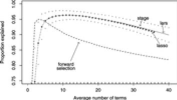
Figure 5: Simulation study comparing LARS, Lasso and Stagewise algorithms; $100$ replications of model (44)–(45). Solid curve shows average proportion explained, (46), for LARS estimates as function of number of steps $k=1,2,\ldots,40$; Lasso and Stagewise give nearly identical results; small dots indicate plus or minus one standard deviation over the $100$ simulations. Classic Forward Selection (heavy dashed curve) rises and falls more abruptly.

Figure 5’s most striking message is that the three algorithms performed almost identically, and rather well. The average proportion explained rises quickly, reaching a maximum of 0.963 at $k=10$, and then declines slowly as $k$ grows to 40. The light dots display the small standard deviation of $\operatorname{pe}(\widehat{\bolds{\mu}}^{(k)\ast})$ over the 100 simulations, roughly $\pm 0.02$. Stopping at any point between $k=5$ and 25 typically gave a $\widehat{\bolds{\mu}}^{(k)\ast}$ with true predictive $R^{2}$ about $0.40$, compared to the ideal value $0.416$ for ${\bolds{\mu}}$.

The dashed curve in Figure 5 tracks the average proportion explained by classic Forward Selection. It rises very quickly, to a maximum of $0.950$ after $k=3$ steps, and then falls back more abruptly than the LARS–Lasso–Stagewise curves. This behavior agrees with the characterization of Forward Selection as a dangerously greedy algorithm.

3.4 Other LARS modifications.

Here are a few more examples of LARS type model-building algorithms.

Constraint (5) can be strengthened to

$$\quad\mbox{minimize}\quad S(\widehat{\bolds}{\beta})\qquad\mbox{subject to}\quad T(\widehat{\bolds}{\beta})\leq t\mbox{ and all }\widehat{\beta}_{j}\geq 0.$$ (47)

This would be appropriate if the statisticians or scientists believed that the variables $x_{j}$ must enter the prediction equation in their defined directions. Situation (47) is a more difficult quadratic programming problem than (5), but it can be solved by a further modification of the Lasso-modified LARS algorithm: change $|\widehat{c}_{j}|$ to $\widehat{c}_{j}$ at both places in (16), set $s_{j}=1$ instead of (17) and change (20) to

$$\widehat{\gamma}=\min_{j\in{\mathcal{A}}^{c}}{}^{\!\!+}\biggl{\{}\frac{\widehat{C}-\widehat{c}_{j}}{A_{\mathcal{A}}-a_{j}}\biggr{\}}.$$ (48)

The positive Lasso usually does not converge to the full OLS solution $\bar{\beta}_{m}$, even for very large choices of $t$.

The changes above amount to considering the ${\bf x}_{j}$ as generating half-lines rather than full one-dimensional spaces. A positive Stagewise version can be developed in the same way, and has the property that the $\widehat{\beta}_{j}$ tracks are always monotone.

LARS–OLS hybrid.

After $k$ steps the LARS algorithm has identified a set ${\mathcal{A}}_{k}$ of covariates, for example, ${\mathcal{A}}_{4}=\{3,9,4,7\}$ in the diabetes study. Instead of $\widehat{\bolds{\beta}}_{k}$ we might prefer $\bar{\bolds{\beta}}_{k}$, the OLS coefficients based on the linear model with covariates in ${\mathcal{A}}_{k}$—using LARS to find the model but not to estimate the coefficients. Besides looking more familiar, this will always increase the usual empirical $R^{2}$ measure of fit (though not necessarily the true fitting accuracy),

$$R^{2}(\bar{\bolds{\beta}}_{k})-R^{2}(\widehat{\bolds{\beta}}_{k})=\frac{1-\rho^{2}_{k}}{\rho_{k}(2-\rho_{k})}[R^{2}(\widehat{\bolds{\beta}}_{k})-R^{2}(\widehat{\bolds{\beta}}_{k-1})],$$ (49)

where $\rho_{k}=\widehat{\gamma}_{k}/\bar{\gamma}_{k}$ as in (29).

The increases in $R^{2}$ were small in the diabetes example, on the order of 0.01 for $k\geq 4$ compared with $R^{2}\ \dot{=}\ 0.50$, which is expected from (49) since we would usually continue LARS until $R^{2}(\widehat{\bolds{\beta}}_{k})-R^{2}(\widehat{\bolds{\beta}}_{k-1})$ was small. For the same reason $\bar{\bolds{\beta}}_{k}$ and $\widehat{\bolds{\beta}}_{k}$ are likely to lie near each other as they did in the diabetes example.

Main effects first.

It is straightforward to restrict the order in which variables are allowed to enter the LARS algorithm. For example, having obtained ${\mathcal{A}}_{4}=\{3,9,4,7\}$ for the diabetes study, we might then wish to check for interactions. To do this we begin LARS again, replacing ${\bf y}$ with ${\bf y}-\widehat{\bolds{\mu}}_{4}$ and ${\bf x}$ with the $n\times 6$ matrix whose columns represent the interactions ${\bf x}_{3:9},{\bf x}_{3:4},\ldots,{\bf x}_{4:7}$.

Backward Lasso.

The Lasso–modified LARS algorithm can be run backward, starting from the full OLS solution $\bar{\bolds{\beta}}_{m}$. Assuming that all the coordinates of $\bar{\bolds{\beta}}_{m}$ are nonzero, their signs must agree with the signs $s_{j}$ that the current correlations had during the final LARS step. This allows us to calculate the last equiangular direction ${\bf u}_{\mathcal{A}}$, (11)–(13). Moving backward from $\widehat{\bolds{\mu}}_{m}=X\bar{\bolds{\beta}}_{m}$ along the line ${\bolds{\mu}}(\gamma)=\widehat{\bolds{\mu}}_{m}-\gamma{\bf u}_{\mathcal{A}}$, we eliminate from the active set the index of the first $\widehat{\beta}_{j}$ that becomes zero. Continuing backward, we keep track of all coefficients $\widehat{\beta}_{j}$ and current correlations $\widehat{c}_{j}$, following essentially the same rules for changing ${\mathcal{A}}$ as in Section 30. As in (10), (34) the calculation of $\widetilde{\gamma}$ and $\widehat{\gamma}$ is easy.

The crucial property of the Lasso that makes backward navigation possible is (30), which permits calculation of the correct equiangular direction ${\bf u}_{\mathcal{A}}$ at each step. In this sense Lasso can be just as well thought of as a backward-moving algorithm. This is not the case for LARS or Stagewise, both of which are inherently forward-moving algorithms.

4 Degrees of freedom and $C_{p}$ estimates.

Figures 1 and 3 show all possible Lasso, Stagewise or LARS estimates of the vector $\bolds{\beta}$ for the diabetes data. The scientists want just a single $\widehat{\bolds{\beta}}$ of course, so we need some rule for selecting among the possibilities. This section concerns a $C_{p}$-type selection criterion, especially as it applies to the choice of LARS estimate.

Let $\widehat{\bolds{\mu}}=g({\bf y})$ represent a formula for estimating ${\bolds{\mu}}$ from the data vector ${\bf y}$. Here, as usual in regression situations, we are considering the covariate vectors ${\bf x}_{1},{\bf x}_{2},\ldots,{\bf x}_{m}$ fixed at their observed values. We assume that given the ${\bf x}$’s, ${\bf y}$ is generated according to an homoskedastic model

$${\bf y}\sim({\bolds{\mu}},\sigma^{2}{\bf I}),$$ (50)

meaning that the components $y_{i}$ are uncorrelated, with mean $\mu_{i}$ and variance $\sigma^{2}$. Taking expectations in the identity

$$(\widehat{\mu}_{i}-\mu_{i})^{2}=(y_{i}-\widehat{\mu}_{i})^{2}-(y_{i}-\mu_{i})^{2}+2(\widehat{\mu}_{i}-\mu_{i})(y_{i}-\mu_{i}),$$ (51)

and summing over $i$, yields

$$E\biggl{\{}\frac{\|\widehat{\bolds{\mu}}-{\bolds{\mu}}\|^{2}}{\sigma^{2}}\biggr{\}}=E\biggl{\{}\frac{\|{\bf y}-\widehat{\bolds{\mu}}\|^{2}}{\sigma^{2}}-n\biggr{\}}+2\sum_{i=1}^{n}\frac{\operatorname{cov}(\widehat{\mu}_{i},y_{i})}{\sigma^{2}}.$$ (52)

The last term of (52) leads to a convenient definition of the degrees of freedom for an estimator $\widehat{\bolds{\mu}}=g({\bf y})$,

$$df_{\mu,\sigma^{2}}=\sum_{i=1}^{n}\operatorname{cov}(\widehat{\mu}_{i},y_{i})/\sigma^{2},$$ (53)

and a $C_{p}$-type risk estimation formula,

$$C_{p}(\widehat{\bolds{\mu}})=\frac{\|{\bf y}-\widehat{\bolds{\mu}}\|^{2}}{\sigma^{2}}-n+2df_{\mu,\sigma^{2}}.$$ (54)

If $\sigma^{2}$ and $df_{\mu,\sigma^{2}}$ are known, $C_{p}(\widehat{\bolds{\mu}})$ is an unbiased estimator of the true risk $E\{\|\widehat{\bolds{\mu}}-{\bolds{\mu}}\|^{2}/\sigma^{2}\}$. For linear estimators $\widehat{\bolds{\mu}}=M{\bf y}$, model (50) makes $df_{\mu,\sigma^{2}}={\rm trace}(M)$, equaling the usual definition of degrees of freedom for OLS, and coinciding with the proposal of Mallows (1973). Section 6 of Efron and Tibshirani (1997) and Section 7 of Efron (1986) discuss formulas (53) and (54) and their role in $C_{p}$, Akaike information criterion (AIC) and Stein’s unbiased risk estimated (SURE) estimation theory, a more recent reference being Ye (1998).

Practical use of $C_{p}$ formula (54) requires preliminary estimates of ${\bolds{\mu}},\sigma^{2}$ and $df_{\mu,\sigma^{2}}$. In the numerical results below, the usual OLS estimates $\bar{{\bolds{\mu}}}$ and $\bar{\sigma}^{2}$ from the full OLS model were used to calculate bootstrap estimates of $df_{\mu,\sigma^{2}}$; bootstrap samples ${\bf y}^{\ast}$ and replications $\widehat{\bolds{\mu}}^{\ast}$ were then generated according to

$${\bf y}^{\ast}\sim N(\bar{{\bolds{\mu}}},\bar{\sigma}^{2})\quad\mbox{and}\quad\widehat{\bolds{\mu}}^{\ast}=g({\bf y}^{\ast}).$$ (55)

Independently repeating (55) say $B$ times gives straightforward estimates for the covariances in (53),

$$\qquad\widehat{\operatorname}{cov}_{i}=\frac{\sum_{b=1}^{B}\widehat{\bolds{\mu}}_{i}^{\ast}(b)[\,{\bf y}_{i}^{\ast}(b)-{\bf y}_{i}^{\ast}(\cdot)]}{B-1},\qquad\mbox{where }{\bf y}^{\ast}(\cdot)=\frac{\sum_{b=1}^{B}{\bf y}^{\ast}(b)}{B},$$ (56)

and then

$$\widehat{df}=\sum_{i=1}^{n}\widehat{\operatorname}{cov}_{i}/\bar{\sigma}^{2}.$$ (57)

Normality is not crucial in (55). Nearly the same results were obtained using ${\bf y}^{\ast}=\bar{{\bolds{\mu}}}^{\ast}+{\bf e}^{\ast}$, where the components of ${\bf e}^{\ast}$ were resampled from ${\bf e}={\bf y}-\bar{{\bolds{\mu}}}$.

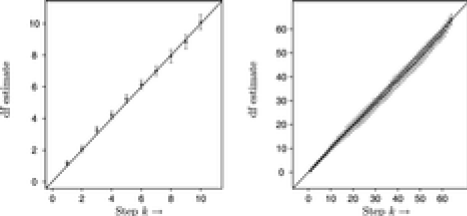
Figure 6: Degrees of freedom for LARS estimates $\widehat{{\bolds{\mu}}}_{k}$: (left) diabetes study, Table $1$, $k=1,\allowbreak 2,\ldots,m=10$; (right) quadratic model (44) for the diabetes data, $m=64$. Solid line is simple approximation $df_{k}=k$. Dashed lines are approximate $95\%$ confidence intervals for the bootstrap estimates. Each panel based on $B=500$ bootstrap replications.

The left panel of Figure 6 shows $\widehat{df}_{\!k}$ for the diabetes data LARS estimates $\widehat{{\bolds{\mu}}}_{k},k=1,2,\ldots,m=10$. It portrays a startlingly simple situation that we will call the “simple approximation,”

$$df(\widehat{{\bolds{\mu}}}_{k})\ \dot{=}\ k.$$ (58)

The right panel also applies to the diabetes data, but this time with the quadratic model (44), having $m=64$ predictors. We see that the simple approximation (58) is again accurate within the limits of the bootstrap computation (57), where $B=500$ replications were divided into 10 groups of 50 each in order to calculate Student-$t$ confidence intervals.

If (58) can be believed, and we will offer some evidence in its behalf, we can estimate the risk of a $k$-step LARS estimator $\widehat{{\bolds{\mu}}}_{k}$ by

$$C_{p}(\widehat{{\bolds{\mu}}}_{k})\ \dot{=}\ \|{\bf y}-\widehat{{\bolds{\mu}}}_{k}\|^{2}/\bar{\sigma}^{2}-n+2k.$$ (59)

The formula, which is the same as the $C_{p}$ estimate of risk for an OLS estimator based on a subset of $k$ preselected predictor vectors, has the great advantage of not requiring any further calculations beyond those for the original LARS estimates. The formula applies only to LARS, and not to Lasso or Stagewise.

Figure 7 displays $C_{p}(\widehat{\bolds{\mu}}_{k})$ as a function of $k$ for the two situations of Figure 6. Minimum $C_{p}$ was achieved at steps $k=7$ and $k=16$, respectively. Both of the minimum $C_{p}$ models looked sensible, their first several selections of “important” covariates agreeing with an earlier model based on a detailed inspection of the data assisted by medical expertise.

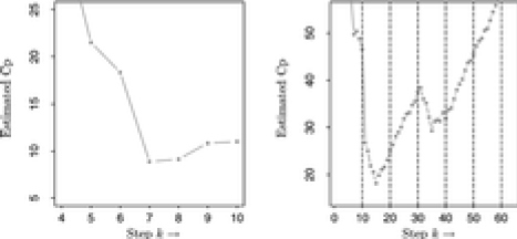
Figure 7: $C_{p}$ estimates of risk (59) for the two situations of Figure 6: (left) $m=10$ model has smallest $C_{p}$ at $k=7$; (right) $m=64$ model has smallest $C_{p}$ at $k=16$.

The simple approximation becomes a theorem in two cases.

Theorem 3.

If the covariate vectors ${\bf x}_{1},{\bf x}_{2},\ldots,{\bf x}_{m}$ are mutually orthogonal, then the $k$-step LARS estimate $\hat{\bolds{\mu}}_{k}$ has $df(\hat{\bolds{\mu}}_{k})=k$.

To state the second more general setting we introduce the following condition. For all possible subsets $X_{{\mathcal{A}}}$ of the full design matrix $X$,

$$G_{{\mathcal{A}}}^{-1}\bolds{1}_{{\mathcal{A}}}>0,$$ (60)

where the inequality is taken element-wise.

The positive cone condition holds if $X$ is orthogonal. It is strictly more general than orthogonality, but counterexamples (such as the diabetes data) show that not all design matrices $X$ satisfy it.

It is also easy to show that LARS, Lasso and Stagewise all coincide under the positive cone condition, so the degrees-of-freedom formula applies to them too in this case.

Theorem 4.

Under the positive cone condition, $df(\hat{\bolds{\mu}}_{k})=k$.

The proof, which appears later in this section, is an application of Stein’s unbiased risk estimate (SURE) [Stein (1981)]. Suppose that $g\dvtx\mathbb{R}^{n}\rightarrow\mathbb{R}^{n}$ is almost differentiable (see Remark A.1 in the Appendix) and set $\nabla\cdot g=\sum_{i=1}^{n}\partial g_{i}/\partial x_{i}.$ If ${\bf y}\sim N_{n}({\bolds{\mu}},\sigma^{2}{\bf I})$, then Stein’s formula states that

$$\sum_{i=1}^{n}\mbox{cov}(g_{i},y_{i})/\sigma^{2}=E[\nabla\cdot g({\bf y})].$$ (61)

The left-hand side is $df(g)$ for the general estimator $g({\bf y})$. Focusing specifically on LARS, it will turn out that $\nabla\cdot\hat{\bolds{\mu}}_{k}({\bf y})=k$ in all situations with probability 1, but that the continuity assumptions underlying (61) and SURE can fail in certain nonorthogonal cases where the positive cone condition does not hold.

A range of simulations suggested that the simple approximation is quite accurate even when the ${\bf x}_{j}$’s are highly correlated and that it requires concerted effort at pathology to make $df(\widehat{\bolds{\mu}}_{k})$ much different than $k$.

Stein’s formula assumes normality, ${\bf y}\sim N({\bolds{\mu}},\sigma^{2}{\bf I})$. A cruder “delta method” rationale for the simple approximation requires only homoskedasticity, (50). The geometry of Figure 4 implies

$$\widehat{\bolds{\mu}}_{k}=\bar{\bf y}_{k}-{\rm cot}_{k}\cdot\|\bar{\bf y}_{k+1}-\bar{\bf y}_{k}\|,$$ (62)

where ${\rm cot}_{k}$ is the cotangent of the angle between ${\bf u}_{k}$ and ${\bf u}_{k+1}$,

$${\rm cot}_{k}=\frac{{\bf u}_{k}^{\prime}{\bf u}_{k+1}}{[1-({\bf u}_{k}^{\prime}{\bf u}_{k+1})^{2}]^{1/2}}.$$ (63)

Let ${\bf v}_{k}$ be the unit vector orthogonal to ${\mathcal{L}}(X_{b})$, the linear space spanned by the first $k$ covariates selected by LARS, and pointing into ${\mathcal{L}}(X_{k+1})$ along the direction of $\bar{\bf y}_{k+1}-\bar{\bf y}_{k}$. For ${\bf y}^{\ast}$ near ${\bf y}$ we can reexpress (62) as a locally linear transformation,

$$\widehat{\bolds{\mu}}_{k}^{\ast}=\widehat{\bolds{\mu}}_{k}+M_{k}({\bf y}^{\ast}-{\bf y})\qquad\mbox{with }M_{k}=P_{k}-{\rm cot}_{k}\cdot{\bf u}_{k}{\bf v}_{k}^{\prime},$$ (64)

$P_{k}$ being the usual projection matrix from $\mathbb{R}^{n}$ into ${\mathcal{L}}(X_{k})$; (64) holds within a neighborhood of ${\bf y}$ such that the LARS choices ${\mathcal{L}}(X_{k})$ and ${\bf v}_{k}$ remain the same.

The matrix $M_{k}$ has trace$(M_{k})=k$. Since the trace equals the degrees of freedom for linear estimators, the simple approximation (58) is seen to be a delta method approximation to the bootstrap estimates (55) and (56).

It is clear that (58) $df(\widehat{{\bolds{\mu}}}_{k})\ \dot{=}\ k$ cannot hold for the Lasso, since the degrees of freedom is $m$ for the full model but the total number of steps taken can exceed $m$. However, we have found empirically that an intuitively plausible result holds: the degrees of freedom is well approximated by the number of nonzero predictors in the model. Specifically, starting at step 0, let $\ell(k)$ be the index of the last model in the Lasso sequence containing $k$ predictors. Then $df(\widehat{{\bolds{\mu}}}_{\ell(k)})\ \dot{=}\ k$. We do not yet have any mathematical support for this claim.

4.1 Orthogonal designs.

In the orthogonal case, we assume that ${\bf x}_{j}={\bf e}_{j}$ for $j=1,\ldots,m$. The LARS algorithm then has a particularly simple form, reducing to soft thresholding at the order statistics of the data.

To be specific, define the soft thresholding operation on a scalar $y_{1}$ at threshold $t$ by

$$\eta(y_{1};t)=\cases{y_{1}-t,&\quad\mbox{if }$y_{1}>t$,\cr 0,&\quad\mbox{if }$|y_{1}|\leq t$,\cr y_{1}+t,&\quad\mbox{if }$y_{1}<-t$.}$$

The order statistics of the absolute values of the data are denoted by

$$|y|_{(1)}\geq|y|_{(2)}\geq\cdots\geq|y|_{(n)}\geq|y|_{(n+1)}:=0.$$ (65)

We note that $y_{m+1},\ldots,y_{n}$ do not enter into the estimation procedure, and so we may as well assume that $m=n.$

Lemma 4.1.

For an orthogonal design with ${\bf x}_{j}={\bf e}_{j},j=1,\ldots,n$, the $k$th LARS estimate ($0\leq k\leq n$) is given by

$$\hat{\mu}_{k,i}({\bf y}) = \cases{y_{i}-|y|_{(k+1)},&\quad\mbox{if }$y_{i}>|y|_{(k+1)}$,\cr 0,&\quad\mbox{if }$|y_{i}|\leq|y|_{(k+1)}$,\cr y_{i}+|y|_{(k+1)},&\quad\mbox{if }$y_{i}<-|y|_{(k+1)}$,}$$ (66)

$$= \eta\bigl{(}y_{i};|y|_{(k+1)}\bigr{)}.$$ (67)

The proof is by induction, stepping through the LARS sequence. First note that the LARS parameters take a simple form in the orthogonal setting:

$$G_{\mathcal{A}}=I_{\mathcal{A}},\qquad A_{\mathcal{A}}=|{\mathcal{A}}|^{-1/2},\qquad{\bf u}_{\mathcal{A}}=|{\mathcal{A}}|^{-1/2}\bolds{1}_{\mathcal{A}},\qquad a_{k,j}=0,\qquad j\notin{\mathcal{A}}_{k}.$$

We assume for the moment that there are no ties in the order statistics (65), so that the variables enter one at a time. Let $j(l)$ be the index corresponding to the $l$th order statistic, $|y|_{(l)}=s_{l}y_{j(l)}$: we will see that ${\mathcal{A}}_{k}=\{j(1),\ldots,j(k)\}.$

We have ${\bf x}_{j}^{\prime}{\bf y}=y_{j}$, and so at the first step LARS picks variable $j(1)$ and sets $\hat{C}_{1}=|y|_{(1)}.$ It is easily seen that

$$\hat{\gamma}_{1}=\min_{j\neq j(1)}\bigl{\{}|y|_{(1)}-|y_{j}|\bigr{\}}=|y|_{(1)}-|y|_{(2)}$$

and so

$$\hat{\bolds{\mu}}_{1}=\bigl{[}|y|_{(1)}-|y|_{(2)}\bigr{]}{\bf e}_{j(1)},$$

which is precisely (66) for $k=1$.

Suppose now that step $k-1$ has been completed, so that ${\mathcal{A}}_{k}=\{j(1),\ldots,j(k)\}$ and (66) holds for $\hat{\bolds{\mu}}_{k-1}$. The current correlations $\hat{C}_{k}=|y|_{(k)}$ and $\hat{c}_{k,j}=y_{j}$ for $j\notin{\mathcal{A}}_{k}$. Since $A_{k}-a_{k,j}=k^{-1/2}$, we have

$$\hat{\gamma}_{k}=\min_{j\notin{\mathcal{A}}_{k}}k^{1/2}\bigl{\{}|y|_{(k)}-|y_{j}|\bigr{\}}$$

and

$$\hat{\gamma}_{k}{\bf u}_{k}=\bigl{[}|y|_{(k)}-|y|_{(k+1)}\bigr{]}\bolds{1}\{j\in{\mathcal{A}}_{k}\}.$$

Adding this term to $\hat{\bolds{\mu}}_{k-1}$ yields (66) for step $k$.

The argument clearly extends to the case in which there are ties in the order statistics (65): if $|y|_{(k+1)}=\cdots=|y|_{(k+r)}$, then ${\mathcal{A}}_{k}({\bf y})$ expands by $r$ variables at step $k+1$ and $\hat{\bolds{\mu}}_{k+\nu}({\bf y}),\nu=1,\ldots,r$, are all determined at the same time and are equal to $\hat{\bolds{\mu}}_{k+1}({\bf y})$.

Proof of Theorem 4 (Orthogonal case) The argument is particularly simple in this setting, and so worth giving separately. First we note from (66) that $\hat{\bolds{\mu}}_{k}$ is continuous and Lipschitz$(1)$ and so certainly almost differentiable. Hence (61) shows that we simply have to calculate $\nabla\cdot\hat{\bolds{\mu}}_{k}$. Inspection of (66) shows that

$$\nabla\cdot\hat{\bolds{\mu}}_{k} = \sum_{i}\frac{\partial\hat{\mu}_{k,i}}{\partial y_{i}}({\bf y})$$

$$= \sum_{i}I\bigl{\{}|y_{i}|>|y|_{(k+1)}\bigr{\}}=k$$

almost surely, that is, except for ties. This completes the proof.

4.2 The divergence formula.

While for the most general design matrices $X$, it can happen that $\hat{\bolds{\mu}}_{k}$ fails to be almost differentiable, we will see that the divergence formula

$$\nabla\cdot\hat{\bolds{\mu}}_{k}({\bf y})=k$$ (68)

does hold almost everywhere. Indeed, certain authors [e.g., Meyer and Woodroofe (2000)] have argued that the divergence $\nabla\cdot\widehat{{\bolds{\mu}}}$ of an estimator provides itself a useful measure of the effective dimension of a model.

Turning to LARS, we shall say that $\hat{{\bolds{\mu}}}({\bf y})$ is locally linear at a data point $y_{0}$ if there is some small open neighborhood of $y_{0}$ on which $\hat{{\bolds{\mu}}}({\bf y})=M{\bf y}$ is exactly linear. Of course, the matrix $M=M(y_{0})$ can depend on $y_{0}$—in the case of LARS, it will be seen to be constant on the interior of polygonal regions, with jumps across the boundaries. We say that a set $G$ has full measure if its complement has Lebesgue measure zero.

Lemma 4.2.

There is an open set $G_{k}$ of full measure such that, at all ${\bf y}\in G_{k}$, $\hat{{\bolds{\mu}}}_{k}({\bf y})$ is locally linear and $\nabla\cdot\hat{\bolds{\mu}}_{k}({\bf y})=k$.

We give here only the part of the proof that relates to actual calculation of the divergence in (68). The arguments establishing continuity and local linearity are delayed to the Appendix.

So, let us fix a point ${\bf y}$ in the interior of $G_{k}$. From Lemma A.1 in the Appendix, this means that near ${\bf y}$ the active set ${\mathcal{A}}_{k}({\bf y})$ is locally constant, that a single variable enters at the next step, this variable being the same near ${\bf y}$. In addition, $\hat{\bolds{\mu}}_{k}({\bf y})$ is locally linear, and hence in particular differentiable. Since $G_{k}\subset G_{l}$ for $l<k$, the same story applies at all previous steps and we have

$$\hat{\bolds{\mu}}_{k}({\bf y})=\sum_{l=1}^{k}\gamma_{l}({\bf y}){\bf u}_{l}.$$ (69)

Differentiating the $j$th component of vector $\hat{\bolds{\mu}}_{k}({\bf y})$ yields

$$\frac{\partial\hat{\mu}_{k,j}}{\partial y_{i}}({\bf y})=\sum_{l=1}^{k}\frac{\partial\gamma_{l}({\bf y})}{\partial y_{i}}u_{l,j}.$$

In particular, for the divergence

$$\nabla\cdot\hat{\bolds{\mu}}_{k}({\bf y})=\sum_{i=1}^{n}\ \frac{\partial\hat{\mu}_{k,i}}{\partial y_{i}}=\sum_{l=1}^{k}\ \langle\nabla\gamma_{l},{\bf u}_{l}\rangle,$$ (70)

the brackets indicating inner product.

The active set is ${\mathcal{A}}_{k}=\{1,2,\ldots,k\}$ and ${\bf x}_{k+1}$ is the variable to enter next. For $k\geq 2,$ write $\bolds{\delta}_{k}={\bf x}_{l}-{\bf x}_{k}$ for any choice $l<k$—as remarked in the Conventions in the Appendix, the choice of $l$ is immaterial (e.g., $l=1$ for definiteness). Let $b_{k+1}=\langle\bolds{\delta}_{k+1},{\bf u}_{k}\rangle$, which is nonzero, as argued in the proof of Lemma A.1. As shown in (A.145) in the Appendix, (2.13) can be rewritten

$$\gamma_{k}({\bf y})=b_{k+1}^{-1}\langle\bolds{\delta}_{k+1},{\bf y}-\hat{\bolds{\mu}}_{k-1}\rangle.$$ (71)

For $k\geq 2$, define the linear space of vectors equiangular with the active set

$${\mathcal{L}}_{k}={\mathcal{L}}_{k}({\bf y})=\bigl{\{}{\bf u}\dvtx\langle{\bf x}_{1},{\bf u}\rangle=\cdots=\langle{\bf x}_{k},{\bf u}\rangle\ \mbox{ for }{\bf x}_{l}\mbox{ with }l\in{\mathcal{A}}_{k}({\bf y})\bigr{\}}.$$

[We may drop the dependence on ${\bf y}$ since ${\mathcal{A}}_{k}({\bf y})$ is locally fixed.] Clearly $\mbox{dim}\,{\mathcal{L}}_{k}=n-k+1$ and

$${\bf u}_{k}\in{\mathcal{L}}_{k},\qquad{\mathcal{L}}_{k+1}\subset{\mathcal{L}}_{k}.$$ (72)

We shall now verify that, for each $k\geq 1$,

$$\langle\nabla\gamma_{k},{\bf u}_{k}\rangle=1\quad\mbox{and}\quad\langle\nabla\gamma_{k},{\bf u}\rangle=0\qquad\mbox{for }{\bf u}\in{\mathcal{L}}_{k+1}.$$ (73)

Formula (70) shows that this suffices to prove Lemma 4.2.

First, for $k=1$ we have $\gamma_{1}({\bf y})=b_{2}^{-1}\langle\bolds{\delta}_{2},{\bf y}\rangle$ and $\langle\nabla\gamma_{1},{\bf u}\rangle=b_{2}^{-1}\langle\bolds{\delta}_{2},{\bf u}\rangle$, and that

$$\langle\bolds{\delta}_{2},{\bf u}\rangle=\langle{\bf x}_{1}-{\bf x}_{2},{\bf u}\rangle=\cases{b_{2},&\quad\mbox{if } ${\bf u}={\bf u}_{1}$,\cr 0,&\quad\mbox{if } ${\bf u}\in{\mathcal{L}}_{2}$.}$$

Now, for general $k$, combine (71) and (69):

$$b_{k+1}\gamma_{k}({\bf y})=\langle\bolds{\delta}_{k+1},{\bf y}\rangle-\sum_{l=1}^{k-1}\langle\bolds{\delta}_{k+1},{\bf u}_{l}\rangle\gamma_{l}({\bf y}),$$

and hence

$$b_{k+1}\langle\nabla\gamma_{k},{\bf u}\rangle=\langle\bolds{\delta}_{k+1},{\bf u}\rangle-\sum_{l=1}^{k-1}\langle\bolds{\delta}_{k+1},{\bf u}_{l}\rangle\langle\nabla\gamma_{l},{\bf u}\rangle.$$

From the definitions of $b_{k+1}$ and ${\mathcal{L}}_{k+1}$ we have

$$\langle\bolds{\delta}_{k+1},{\bf u}\rangle=\langle{\bf x}_{l}-{\bf x}_{k+1}\rangle=\cases{b_{k+1},&\quad\mbox{if } ${\bf u}={\bf u}_{k}$,\cr 0,&\quad\mbox{if } ${\bf u}\in{\mathcal{L}}_{k+1}$.}$$

Hence the truth of (73) for step $k$ follows from its truth at step $k-1$ because of the containment properties (72).

4.3 Proof of Theorem 4.

To complete the proof of Theorem 4, we state the following regularity result, proved in the Appendix.

Lemma 4.3.

Under the positive cone condition, $\hat{\bolds{\mu}}_{k}({\bf y})$ is continuous and almost differentiable.

This guarantees that Stein’s formula (61) is valid for $\hat{\bolds{\mu}}_{k}$ under the positive cone condition, so the divergence formula of Lemma 4.2 then immediately yields Theorem 4.

5 LARS and Lasso properties.

The LARS and Lasso algorithms are described more carefully in this section, with an eye toward fully understanding their relationship. Theorem 1 of Section 3 will be verified. The latter material overlaps results in Osborne, Presnell and Turlach (2000a), particularly in their Section 4. Our point of view here allows the Lasso to be described as a quite simple modification of LARS, itself a variation of traditional Forward Selection methodology, and in this sense should be more accessible to statistical audiences. In any case we will stick to the language of regression and correlation rather than convex optimization, though some of the techniques are familiar from the optimization literature.

The results will be developed in a series of lemmas, eventually lending to a proof of Theorem 1 and its generalizations. The first three lemmas refer to attributes of the LARS procedure that are not specific to its Lasso modification.

Using notation as in (24)–(27), suppose LARS has completed step $k-1$, giving estimate $\widehat{\bolds{\mu}}_{k-1}$ and active set ${\mathcal{A}}_{k}$ for step $k$, with covariate ${\bf x}_{k}$ the newest addition to the active set.

Lemma 5.1.

If ${\bf x}_{k}$ is the only addition to the active set at the end of step $k-1$, then the coefficient vector $w_{k}=A_{k}{\mathcal{G}}_{k}^{-1}\bolds{1}_{k}$ for the equiangular vector ${\bf u}_{k}=X_{k}w_{k}$, (13), has its $k$th component $w_{kk}$ agreeing in sign with the current correlation $c_{kk}={\bf x}_{k}^{\prime}({\bf y}-\widehat{\bolds{\mu}}_{k-1})$. Moreover, the regression vector $\widehat{\bolds}{\beta}_{k}$ for $\widehat{\bolds{\mu}}_{k}=X\widehat{\bolds}{\beta}_{k}$ has its $k$th component $\widehat{\beta}_{kk}$ agreeing in sign with $c_{kk}$.

Lemma 5.1 says that new variables enter the LARS active set in the “correct” direction, a weakened version of the Lasso requirement (30). This will turn out to be a crucial connection for the LARS–Lasso relationship.

Proof of Lemma 4 The case $k=1$ is apparent. Note that since

$$X_{k}^{\prime}({\bf y}-\widehat{\bolds{\mu}}_{k-1})=\widehat{C}_{k}{\bf 1}_{k},$$

(27), from (13) we have

$$w_{k}=A_{k}\widehat{C}_{k}^{-1}[(X_{k}^{\prime}X_{k})^{-1}X_{k}^{\prime}({\bf y}-\widehat{\bolds{\mu}}_{k-1})]:=A_{k}\widehat{C}_{k}^{-1}w_{k}^{*}.$$ (74)

The term in square braces is the least squares coefficient vector in the regression of the current residual on $X_{k}$, and the term preceding it is positive.

Note also that

$$X_{k}^{\prime}({\bf y}-\bar{\bf y}_{k-1})=({\bf 0},\delta)^{\prime}\qquad\mbox{with }\delta>0,$$ (75)

since $X_{k-1}^{\prime}({\bf y}-\bar{\bf y}_{k-1})=\bf{0}$ by definition (this $\bf 0$ has $k-1$ elements), and $c_{k}(\gamma)={\bf x}_{k}^{\prime}({\bf y}-\gamma{\bf u}_{k-1})$ decreases more slowly in $\gamma$ than $c_{j}(\gamma)$ for $j\in{\mathcal{A}}_{k-1}$:

$$c_{k}(\gamma)\cases{<c_{j}(\gamma),&\quad\mbox{for }$\gamma<\widehat{\gamma}_{k-1}$,\cr=c_{j}(\gamma)=\widehat{C}_{k},&\quad\mbox{for }$\gamma=\widehat{\gamma}_{k-1}$,\cr>c_{j}(\gamma),&\quad\mbox{for }$\widehat{\gamma}_{k-1}<\gamma<\bar{\gamma}_{k-1}$.}$$ (76)

Thus

$$\widehat{w}_{k}^{*} = (X_{k}^{\prime}X_{k})^{-1}X_{k}^{\prime}({\bf y}-\bar{\bf y}_{k-1}+\bar{\bf y}_{k-1}-\widehat{\bolds{\mu}}_{k-1})$$ (77)

$$= (X_{k}^{\prime}X_{k})^{-1}\left(\begin{array}[]{c}\bf 0\\ \delta\end{array}\right)+(X_{k}^{\prime}X_{k})^{-1}X_{k}^{\prime}[(\bar{\gamma}_{k-1}-\widehat{\gamma}_{k-1}){\bf u}_{k-1}].$$ (80)

The $k$th element of $\widehat{w}^{*}_{k}$ is positive, because it is in the first term in (80) [$(X_{k}^{\prime}X_{k})$ is positive definite], and in the second term it is $0$ since ${\bf u}_{k-1}\in{\mathcal{L}}(X_{k-1})$.

This proves the first statement in Lemma 5.1. The second follows from

$$\widehat{\beta}_{kk}=\widehat{\beta}_{k-1,k}+\widehat{\gamma}_{k}w_{kk},$$ (81)

and $\widehat{\beta}_{k-1,k}=0,\ {\bf x}_{k}$ not being active before step $k$.

Our second lemma interprets the quantity $A_{\mathcal{A}}=({\bf 1}^{\prime}{\mathcal{G}}_{\mathcal{A}}^{-1}{\bf 1})^{-1/2}$, (11) and (12). Let ${\mathcal{S}}_{\mathcal{A}}$ indicate the extended simplex generated by the columns of $X_{\mathcal{A}}$,

$${\mathcal{S}}_{\mathcal{A}}=\Biggl{\{}{\bf v}=\sum_{j\in{\mathcal{A}}}s_{j}{\bf x}_{j}P_{j}\dvtx\sum_{j\in{\mathcal{A}}}P_{j}=1\Biggr{\}},$$ (82)

“extended” meaning that the coefficients $P_{j}$ are allowed to be negative.

Lemma 5.2.

The point in ${\mathcal{S}}_{\mathcal{A}}$ nearest the origin is

$${\bf v}_{\mathcal{A}}=A_{\mathcal{A}}{\bf u}_{\mathcal{A}}=A_{\mathcal{A}}X_{\mathcal{A}}w_{\mathcal{A}}\qquad\mbox{where }w_{\mathcal{A}}=A_{\mathcal{A}}{\mathcal{G}}_{\mathcal{A}}^{-1}{\bf 1}_{\mathcal{A}},$$ (83)

with length $\|{\bf v}_{\mathcal{A}}\|=A_{\mathcal{A}}$. If ${\mathcal{A}}\subseteq{\mathcal{B}}$, then $A_{\mathcal{A}}\geq A_{\mathcal{B}}$, the largest possible value being $A_{\mathcal{A}}=1$ for ${\mathcal{A}}$ a singleton.

For any ${\bf v}\in{\mathcal{S}}_{\mathcal{A}}$, the squared distance to the origin is $\|X_{\mathcal{A}}P\|^{2}=P^{\prime}{\mathcal{G}}_{\mathcal{A}}P$. Introducing a Lagrange multiplier to enforce the summation constraint, we differentiate

$$P^{\prime}{\mathcal{G}}_{\mathcal{A}}P-\lambda({\bf 1}_{\mathcal{A}}^{\prime}P-1),$$ (84)

and find that the minimizing $P_{\mathcal{A}}=\lambda{\mathcal{G}}_{\mathcal{A}}^{-1}{\bf 1}_{\mathcal{A}}$. Summing, we get $\lambda{\bf 1}_{\mathcal{A}}^{\prime}{\mathcal{G}}_{\mathcal{A}}^{-1}{\bf 1}_{\mathcal{A}}=1$, and hence

$$P_{\mathcal{A}}=A_{\mathcal{A}}^{2}{\mathcal{G}}_{\mathcal{A}}^{-1}{\bf 1}_{\mathcal{A}}=A_{\mathcal{A}}w_{\mathcal{A}}.$$ (85)

Hence ${\bf v}_{\mathcal{A}}=X_{\mathcal{A}}P_{\mathcal{A}}\in{\mathcal{S}}_{\mathcal{A}}$ and

$$\|{\bf v}_{\mathcal{A}}\|^{2}=P_{\mathcal{A}}^{\prime}{\mathcal{G}}_{\mathcal{A}}^{-1}P_{\mathcal{A}}=A_{\mathcal{A}}^{4}{\bf 1}_{\mathcal{A}}^{\prime}{\mathcal{G}}_{\mathcal{A}}^{-1}{\bf 1}_{\mathcal{A}}=A_{\mathcal{A}}^{2},$$ (86)

verifying (83). If ${\mathcal{A}}\subseteq{\mathcal{B}}$, then ${\mathcal{S}}_{\mathcal{A}}\subseteq{\mathcal{S}}_{\mathcal{B}}$, so the nearest distance $A_{\mathcal{B}}$ must be equal to or less than the nearest distance $A_{\mathcal{A}}$. $A_{\mathcal{A}}$ obviously equals $1$ if and only if ${\mathcal{A}}$ has only one member.

The LARS algorithm and its various modifications proceed in piecewise linear steps. For $m$-vectors $\widehat{\bolds}{\beta}$ and d, let

$$\bolds{\beta}(\gamma)=\widehat{\bolds}{\beta}+\gamma{\bf d}\quad\mbox{and}\quad S(\gamma)=\|{\bf y}-X\bolds{\beta}(\gamma)\|^{2}.$$ (87)

Lemma 5.3.

Letting $\widehat{\bf c}=X^{\prime}({\bf y}-X\widehat{\bolds}{\beta})$ be the current correlation vector at $\widehat{\bolds{\mu}}=X\widehat{\bolds}{\beta}$,

$$S(\gamma)-S(0)=-2\,\widehat{\bf c}^{\,\prime}{\bf d}\gamma+{\bf d}^{\prime}X^{\prime}X{\bf d}\gamma^{2}.$$ (88)

${\mathcal{S}}(\gamma)$ is a quadratic function of $\gamma$, with first two derivatives at $\gamma=0$,

$$\dot{S}(0)=-2\,\widehat{\bf c\,}^{\prime}{\bf d}\quad\mbox{and}\quad\ddot{S}(0)=2{\bf d}^{\prime}X^{\prime}X{\bf d}.$$ (89)

The remainder of this section concerns the LARS–Lasso relationship. Now $\widehat{\bolds}{\beta}=\widehat{\bolds}{\beta}(t)$ will indicate a Lasso solution (5), and likewise $\widehat{\bolds{\mu}}=\widehat{\bolds{\mu}}(t)=X\widehat{\bolds}{\beta}(t)$. Because $S(\widehat{\bolds}{\beta})$ and $T(\widehat{\bolds}{\beta})$ are both convex functions of $\widehat{\bolds}{\beta}$, with $S$ strictly convex, standard results show that $\widehat{\bolds}{\beta}(t)$ and $\widehat{\bolds{\mu}}(t)$ are unique and continuous functions of $t$.

For a given value of $t$ let

$${\mathcal{A}}=\{j\dvtx\widehat{\beta}_{j}(t)\neq 0\}.$$ (90)

We will show later that ${\mathcal{A}}$ is also the active set that determines the equiangular direction ${\bf u}_{\mathcal{A}}$, (13), for the LARS–Lasso computations.

We wish to characterize the track of the Lasso solutions $\widehat{\bolds}{\beta}(t)$ or equivalently of $\widehat{\bolds{\mu}}(t)$ as $t$ increases from 0 to its maximum effective value. Let ${\mathcal{T}}$ be an open interval of the $t$ axis, with infimum $t_{0}$, within which the set ${\mathcal{A}}$ of nonzero Lasso coefficients $\widehat{\beta}_{j}(t)$ remains constant.

Lemma 5.4.

The Lasso estimates $\widehat{\bolds{\mu}}(t)$ satisfy

$$\widehat{\bolds{\mu}}(t)=\widehat{\bolds{\mu}}(t_{0})+A_{\mathcal{A}}(t-t_{0}){\bf u}_{\mathcal{A}}$$ (91)

for $t\in{\mathcal{T}}$, where ${\bf u}_{\mathcal{A}}$ is the equiangular vector $X_{\mathcal{A}}w_{\mathcal{A}},w_{\mathcal{A}}=A_{\mathcal{A}}{\mathcal{G}}_{\mathcal{A}}^{-1}{\bf 1}_{\mathcal{A}}$, (14).

The lemma says that, for $t$ in ${\mathcal{T}}$, $\widehat{\bolds{\mu}}(t)$ moves linearly along the equiangular vector ${\bf u}_{\mathcal{A}}$ determined by ${\mathcal{A}}$. We can also state this in terms of the nonzero regression coefficients $\widehat{\beta}_{\mathcal{A}}(t)$,

$$\widehat{\beta}_{\mathcal{A}}(t)=\widehat{\beta}_{\mathcal{A}}(t_{0})+S_{\mathcal{A}}A_{\mathcal{A}}(t-t_{0})w_{\mathcal{A}},$$ (92)

where $S_{\mathcal{A}}$ is the diagonal matrix with diagonal elements $s_{j}$, $j\in{\mathcal{A}}$. [$S_{\mathcal{A}}$ is needed in (92) because definitions (11), (17) require $\widehat{\bolds{\mu}}(t)=X\widehat{\bolds}{\beta}(t)=X_{\mathcal{A}}S_{\mathcal{A}}\widehat{\beta}_{\mathcal{A}}(t)$.]

Since $\widehat{\bolds}{\beta}(t)$ satisfies (5) and has nonzero set ${\mathcal{A}}$, it also minimizes

$$S(\widehat{\beta}_{\mathcal{A}})=\|{\bf y}-X_{\mathcal{A}}S_{\mathcal{A}}\widehat{\beta}_{\mathcal{A}}\|^{2}$$ (93)

subject to

$$\sum_{\mathcal{A}}s_{j}\widehat{\beta}_{j}=t\quad\mbox{and}\quad\operatorname{sign}(\widehat{\beta}_{j})=s_{j}\qquad\mbox{for }j\in{\mathcal{A}}.$$ (94)

[The inequality in (5) can be replaced by $T(\widehat{\bolds}{\beta})=t$ as long as $t$ is less than $\sum|\bar{\beta}_{j}|$ for the full $m$-variable OLS solution $\bar{\bolds{\beta}}_{m}$.] Moreover, the fact that the minimizing point $\widehat{\beta}_{\mathcal{A}}(t)$ occurs strictly inside the simplex (94), combined with the strict convexity of $S(\widehat{\beta}_{\mathcal{A}})$, implies we can drop the second condition in (94) so that $\widehat{\beta}_{\mathcal{A}}(t)$ solves

$$\mbox{minimize}\quad\{S(\widehat{\beta}_{\mathcal{A}})\}\qquad\mbox{subject to}\quad\sum_{\mathcal{A}}s_{j}\widehat{\beta}_{j}=t.$$ (95)

Introducing a Lagrange multiplier, (95) becomes

$$\mbox{minimize}\quad\tfrac{1}{2}\|{\bf y}-X_{\mathcal{A}}S_{\mathcal{A}}\widehat{\beta}_{\mathcal{A}}\|^{2}+\lambda\sum_{\mathcal{A}}s_{j}\widehat{\beta}_{j}.$$ (96)

Differentiating we get

$$-S_{\mathcal{A}}X_{\mathcal{A}}^{\prime}({\bf y}-X_{\mathcal{A}}S_{\mathcal{A}}\widehat{\beta}_{\mathcal{A}})+\lambda S_{\mathcal{A}}{\bf 1}_{\mathcal{A}}=0.$$ (97)

Consider two values $t_{1}$ and $t_{2}$ in ${\mathcal{T}}$ with $t_{0}<t_{1}<t_{2}$. Corresponding to each of these are values for the Lagrange multiplier $\lambda$ such that $\lambda_{1}>\lambda_{2}$, and solutions $\widehat{\beta}_{\mathcal{A}}(t_{1})$ and $\widehat{\beta}_{\mathcal{A}}(t_{2})$. Inserting these into (97), differencing and premultiplying by $S_{\mathcal{A}}$ we get

$$X_{\mathcal{A}}^{\prime}X_{\mathcal{A}}S_{\mathcal{A}}\bigl{(}\widehat{\beta}_{\mathcal{A}}(t_{2})-\widehat{\beta}_{\mathcal{A}}(t_{1})\bigr{)}=(\lambda_{1}-\lambda_{2}){\bf 1}_{\mathcal{A}}.$$ (98)

Hence

$$\widehat{\beta}_{\mathcal{A}}(t_{2})-\widehat{\beta}_{\mathcal{A}}(t_{1})=(\lambda_{1}-\lambda_{2})S_{\mathcal{A}}{\mathcal{G}}_{\mathcal{A}}^{-1}{\bf 1}_{\mathcal{A}}.$$ (99)

However, $s_{\mathcal{A}}^{\prime}[(\widehat{\beta}_{\mathcal{A}}(t_{2})-\widehat{\beta}_{\mathcal{A}}(t_{1})]=t_{2}-t_{1}$ according to the Lasso definition, so

$$\qquad\quad\hskip 5.0ptt_{2}-t_{1}=(\lambda_{1}-\lambda_{2})s_{\mathcal{A}}^{\prime}S_{\mathcal{A}}{\mathcal{G}}_{\mathcal{A}}^{-1}{\bf 1}_{\mathcal{A}}=(\lambda_{1}-\lambda_{2}){\bf 1}_{\mathcal{A}}^{\prime}{\mathcal{G}}_{\mathcal{A}}^{-1}{\bf 1}_{\mathcal{A}}=(\lambda_{1}-\lambda_{2})A_{\mathcal{A}}^{-2}$$ (100)

and

$$\widehat{\beta}_{\mathcal{A}}(t_{2})-\widehat{\beta}_{\mathcal{A}}(t_{1})=S_{\mathcal{A}}A_{\mathcal{A}}^{2}(t_{2}-t_{1}){\mathcal{G}}_{\mathcal{A}}^{-1}{\bf 1}_{\mathcal{A}}=S_{\mathcal{A}}A_{\mathcal{A}}(t-t_{1})w_{\mathcal{A}}.$$ (101)

Letting $t_{2}=t$ and $t_{1}\rightarrow t_{0}$ gives (92) by the continuity of $\widehat{\bolds}{\beta}(t)$, and finally (91). Note that (91) implies that the maximum absolute correlation $\widehat{C}(t)$ equals $\widehat{C}(t_{0})-A_{\mathcal{A}}^{2}(t-t_{0})$, so that $\widehat{C}(t)$ is a piecewise linear decreasing function of the Lasso parameter $t$.

The Lasso solution $\widehat{\bolds}{\beta}(t)$ occurs on the surface of the diamond-shaped convex polytope

$${\mathcal{D}}(t)=\Bigl{\{}\bolds{\beta}\dvtx\sum|\beta_{j}|\leq t\Bigr{\}},$$ (102)

${\mathcal{D}}(t)$ increasing with $t$. Lemma 5.4 says that, for $t\in{\mathcal{T}}$, $\widehat{\bolds}{\beta}(t)$ moves linearly along edge ${\mathcal{A}}$ of the polytope, the edge having $\beta_{j}=0$ for $j\notin{\mathcal{A}}$. Moreover the regression estimates $\widehat{\bolds{\mu}}(t)$ move in the LARS equiangular direction ${\bf u}_{\mathcal{A}}$, (13). It remains to show that “${\mathcal{A}}$” changes according to the rules of Theorem 1, which is the purpose of the next three lemmas.

Lemma 5.5.

A Lasso solution $\widehat{\bolds}{\beta}$ has

$$\widehat{c}_{j}=\widehat{C}\cdot\operatorname{sign}(\widehat{\beta}_{j})\qquad\mbox{for }j\in{\mathcal{A}},$$ (103)

where $\widehat{c}_{j}$ equals the current correlation ${\bf x}_{j}^{\prime}({\bf y}-\widehat{\bolds{\mu}})={\bf x}_{j}^{\prime}({\bf y}-X\widehat{\bolds}{\beta})$. In particular, this implies that

$$\operatorname{sign}(\widehat{\beta}_{j})=\operatorname{sign}(\widehat{c}_{j})\qquad\mbox{for }j\in{\mathcal{A}}.$$ (104)

This follows immediately from (97) by noting that the $j$th element of the left-hand side is $\widehat{c}_{j}$, and the right-hand side is $\lambda\cdot\mbox{sign}(\widehat{\beta}_{j})$ for $j\in\mathcal{A}$. Likewise $\lambda=|\widehat{c}_{j}|=\widehat{C}$.

Lemma 5.6.

Within an interval ${\mathcal{T}}$ of constant nonzero set ${\mathcal{A}}$, and also at $t_{0}=\inf({\mathcal{T}})$, the Lasso current correlations $c_{j}(t)={\bf x}_{j}^{\prime}({\bf y}-\widehat{\bolds{\mu}}(t))$ satisfy

$$|c_{j}(t)|=\widehat{C}(t)\equiv\max\{|c_{\ell}(t)|\}\qquad\mbox{for }j\in{\mathcal{A}}$$

and

$$|c_{j}(t)|\leq\widehat{C}(t)\qquad\mbox{for }j\notin{\mathcal{A}}.$$ (105)

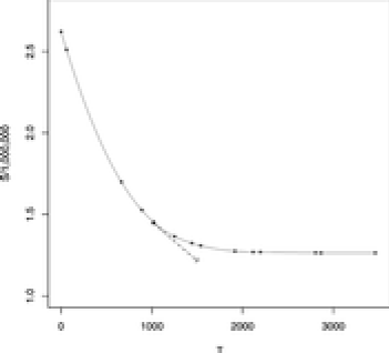
Figure 8: Plot of $S$ versus $T$ for Lasso applied to diabetes data; points indicate the $12$ modified LARS steps of Figure 1; triangle is $(T,S)$ boundary point at $t=1000$; dashed arrow is tangent at $t=1000$, negative slope $R_{t}$, (106). The $(T,S)$ curve is a decreasing, convex, quadratic spline.

Equation (103) says that the $|c_{j}(t)|$ have identical values, say $\widehat{C}_{t}$, for $j\in{\mathcal{A}}$. It remains to show that $\widehat{C}_{t}$ has the extremum properties indicated in (105). For an $m$-vector d we define $\bolds{\beta}(\gamma)=\widehat{\bolds}{\beta}(t)+\gamma{\bf d}$ and $S(\gamma)$ as in (87), likewise $T(\gamma)=\sum|\beta_{j}(\gamma)|$, and

$$R_{t}(d)=-\dot{S}(0)/\dot{T}(0).$$ (106)

Again assuming $\widehat{\beta}_{j}>0$ for $j\in{\mathcal{A}}$, by redefinition of ${\bf x}_{j}$ if necessary, (89) and (103) yield

$$R_{t}({\bf d})=2\Biggl{[}\widehat{C}_{t}\sum_{\mathcal{A}}d_{j}+\sum_{{\mathcal{A}}^{c}}c_{j}(t)d_{j}\Biggr{]}\bigg{/}\Biggl{[}\sum_{\mathcal{A}}d_{j}+\sum_{{\mathcal{A}}^{c}}|d_{j}|\Biggr{]}.\$$ (107)

If $d_{j}=0$ for $j\notin{\mathcal{A}}$, and $\sum d_{j}\neq 0$,

$$R_{t}({\bf d})=2\widehat{C}_{t},$$ (108)

while if ${\bf d}$ has only component $j$ nonzero we can make

$$R_{t}({\bf d})=2|c_{j}(t)|.$$ (109)

According to Lemma 5.4 the Lasso solutions for $t\in{\mathcal{T}}$ use $d_{\mathcal{A}}$ proportional to $w_{\mathcal{A}}$ with $d_{j}=0$ for $j\notin{\mathcal{A}}$, so

$$R_{t}\equiv R_{t}(w_{\mathcal{A}})$$ (110)

is the downward slope of the curve ($T,S(T))$ at $T=t$, and by the definition of the Lasso must maximize $R_{t}({\bf d})$. This shows that $\widehat{C}_{t}=\widehat{C}(t)$, and verifies (105), which also holds at $t_{0}=\inf({\mathcal{T}})$ by the continuity of the current correlations.

We note that Lemmas 5.4–5.6 follow relatively easily from the Karush–Kuhn–Tucker conditions for optimality for the quadratic programming Lasso problem [Osborne, Presnell and Turlach (2000a)]; we have chosen a more geometrical argument here to demonstrate the nature of the Lasso path.

Figure 8 shows the $(T,S)$ curve corresponding to the Lasso estimates in Figure 1. The arrow indicates the tangent to the curve at $t=1000$, which has downward slope $R_{1000}$. The argument above relies on the fact that $R_{t}({\bf d})$ cannot be greater than $R_{t}$, or else there would be $(T,S)$ values lying below the optimal curve. Using Lemmas 3 and 4 it can be shown that the $(T,S)$ curve is always convex, as in Figure 8, being a quadratic spline with $\dot{S}(T)=-2\widehat{C}(T)$ and $\ddot{S}(T)=2A_{\mathcal{A}}^{2}$.

We now consider in detail the choice of active set at a breakpoint of the piecewise linear Lasso path. Let $t=t_{0}$ indicate such a point, $t_{0}=\inf({\mathcal{T}})$ as in Lemma 5.6, with Lasso regression vector $\widehat{\bolds}{\beta}$, prediction estimate $\widehat{\bolds{\mu}}=X\widehat{\bolds}{\beta}$, current correlations $\widehat{\bf c}=X^{\prime}({\bf y}-\widehat{\bolds{\mu}})$, $s_{j}=\operatorname{sign}(\widehat{c}_{j})$ and maximum absolute correlation $\widehat{C}$. Define

$${\mathcal{A}}_{1}=\{j\dvtx\widehat{\beta}_{j}\neq 0\},\qquad{\mathcal{A}}_{0}=\{j\dvtx\widehat{\beta}_{j}=0\mbox{ and }|\widehat{c}_{j}|=\widehat{C}\},$$ (111)

${\mathcal{A}}_{10}={\mathcal{A}}_{1}\cup{\mathcal{A}}_{0}$ and ${\mathcal{A}}_{2}={\mathcal{A}}_{10}^{c}$, and take $\bolds{\beta}(\gamma)=\widehat{\bolds}{\beta}+\gamma{\bf d}$ for some $m$-vector d; also $S(\gamma)=\|{\bf y}-X\bolds{\beta}(\gamma)\|^{2}$ and $T(\gamma)=\sum|\beta_{j}(\gamma)|$.

Lemma 5.7.

The negative slope (106) at $t_{0}$ is bounded by $2\widehat{C}$,

$$R({\bf d})=-\dot{S}(0)/\dot{T}(0)\leq 2\widehat{C},$$ (112)

with equality only if $d_{j}=0$ for $j\in{\mathcal{A}}_{2}$. If so, the differences $\Delta S=S(\gamma)-S(0)$ and $\Delta T=T(\gamma)-T(0)$ satisfy

$$\Delta S=-2\widehat{C}\Delta T+L({\bf d})^{2}\cdot(\Delta T)^{2},$$ (113)

where

$$L({\bf d})=\|X{\bf d}/d_{+}\|.$$ (114)

We can assume $\widehat{c}_{j}\geq 0$ for all $j$, by redefinition if necessary, so $\widehat{\beta}_{j}\geq 0$ according to Lemma 5.5. Proceeding as in (107),

$$R({\bf d})=2\widehat{C}\Biggl{[}\,\sum_{{\mathcal{A}}_{10}}d_{j}+\sum_{{\mathcal{A}}_{2}}(\widehat{c}_{j}/\widehat{C})d_{j}\Biggr{]}\bigg{/}\Biggl{[}\sum_{{\mathcal{A}}_{1}}d_{j}+\sum_{{\mathcal{A}}_{0}\cup{\mathcal{A}}_{2}}|d_{j}|\Biggr{]}.$$ (115)

We need $d_{j}\geq 0$ for $j\in{\mathcal{A}}_{0}\cup{\mathcal{A}}_{2}$ in order to maximize (115), in which case

$$R({\bf d})=2\widehat{C}\Biggl{[}\,\sum_{{\mathcal{A}}_{10}}d_{j}+\sum_{{\mathcal{A}}_{2}}(\widehat{c}_{j}/\widehat{C})d_{j}\Biggr{]}\bigg{/}\Biggl{[}\,\sum_{{\mathcal{A}}_{10}}d_{j}+\sum_{{\mathcal{A}}_{2}}d_{j}\Biggr{]}.$$ (116)

This is $<2\widehat{C}$ unless $d_{j}=0$ for $j\in{\mathcal{A}}_{2}$, verifying (112), and also implying

$$T(\gamma)=T(0)+\gamma\sum_{{\mathcal{A}}_{10}}d_{j}.$$ (117)

The first term on the right-hand side of (88) is then $-2\widehat{C}(\Delta T)$, while the second term equals $({\bf d}/d_{+})^{\prime}X^{\prime}X({\bf d}/d_{+})(\Delta T)^{2}=L({\bf d})^{2}$.

Lemma 5.7 has an important consequence. Suppose that ${\mathcal{A}}$ is the current active set for the Lasso, as in (92), and that ${\mathcal{A}}\subseteq{\mathcal{A}}_{10}$. Then Lemma 5.2 says that $L({\bf d})$ is $\geq A_{\mathcal{A}}$, and (113) gives

$$\Delta S\geq-2\widehat{C}\cdot\Delta T+A_{\mathcal{A}}^{2}\cdot(\Delta T)^{2},$$ (118)

with equality if d is chosen to give the equiangular vector ${\bf u}_{\mathcal{A}}$, $d_{\mathcal{A}}=S_{\mathcal{A}}w_{\mathcal{A}}$, $d_{{\mathcal{A}}^{c}}=0$. The Lasso operates to minimize $S(T)$ so we want $\Delta S$ to be as negative as possible. Lemma 5.7 says that if the support of d is not confined to ${\mathcal{A}}_{10}$, then $\dot{S}(0)$ exceeds the optimum value $-2\widehat{C}$; if it is confined, then $\dot{S}(0)=-2\widehat{C}$ but $\ddot{S}(0)$ exceeds the minimum value $2A_{\mathcal{A}}$ unless $d_{\mathcal{A}}$ is proportional to $S_{\mathcal{A}}w_{\mathcal{A}}$ as in (92).

Suppose that $\widehat{\bolds}{\beta}$, a Lasso solution, exactly equals a $\widehat{\bolds}{\beta}$ obtained from the Lasso-modified LARS algorithm, henceforth called LARS–Lasso, as at $t=1000$ in Figures 1 and 3. We know from Lemma 5.4 that subsequent Lasso estimates will follow a linear track determined by some subset ${\mathcal{A}}$, ${\bolds{\mu}}(\gamma)=\widehat{\bolds{\mu}}+\gamma{\bf u}_{\mathcal{A}}$, and so will the LARS–Lasso estimates, but to verify Theorem 1 we need to show that “${\mathcal{A}}$” is the same set in both cases.

Lemmas 4–7 put four constraints on the Lasso choice of ${\mathcal{A}}$. Define ${\mathcal{A}}_{1}$, ${\mathcal{A}}_{0}$ and ${\mathcal{A}}_{10}$ as at (111).

Constraint 1.

${\mathcal{A}}_{1}\subseteq{\mathcal{A}}$. This follows from Lemma 5.4 since for sufficiently small $\gamma$ the subsequent Lasso coefficients (92),

$$\widehat{\beta}_{\mathcal{A}}(\gamma)=\widehat{\beta}_{\mathcal{A}}+\gamma S_{\mathcal{A}}w_{\mathcal{A}},$$ (119)

will have $\widehat{\beta}_{j}(\gamma)\neq 0,j\in{\mathcal{A}}_{1}$.

Constraint 2.

${\mathcal{A}}\subseteq{\mathcal{A}}_{10}$. Lemma 5.7, (112) shows that the Lasso choice $\widehat{\bf d}$ in $\bolds{\beta}(\gamma)=\widehat{\bolds}{\beta}+\gamma\widehat{\bf d}$ must have its nonzero support in ${\mathcal{A}}_{10}$, or equivalently that $\widehat{\bolds{\mu}}(\gamma)=\widehat{\bolds{\mu}}+\gamma{\bf u}_{\mathcal{A}}$ must have ${\bf u}_{\mathcal{A}}\in{\mathcal{L}}(X_{{\mathcal{A}}_{10}})$. (It is possible that ${\bf u}_{\mathcal{A}}$ happens to equal ${\bf u}_{\mathcal{B}}$ for some ${\mathcal{B}}\supset{\mathcal{A}}_{10}$, but that does not affect the argument below.)

Constraint 3.

$w_{\mathcal{A}}=A_{\mathcal{A}}{\mathcal{G}}_{\mathcal{A}}^{-1}{\bf 1}_{\mathcal{A}}$ cannot have $\operatorname{sign}(w_{j})\neq\operatorname{sign}(\widehat{c}_{j})$ for any coordinate $j\in{\mathcal{A}}_{0}$. If it does, then $\operatorname{sign}(\widehat{\beta}_{j}(\gamma))\neq\mbox{sign}(\widehat{c}_{j}(\gamma))$ for sufficiently small $\gamma$, violating Lemma 5.5.

Constraint 4.

Subject to Constraints 1–3, ${\mathcal{A}}$ must minimize $A_{\mathcal{A}}$. This follows from Lemma 5.7 as in (118), and the requirement that the Lasso curve $S(T)$ declines at the fastest possible rate.

Theorem 1 follows by induction: beginning at $\widehat{\bolds}{\beta}_{0}=0$, we follow the LARS–Lasso algorithm and show that at every succeeding step it must continue to agree with the Lasso definition (5). First of all, suppose that $\widehat{\bolds}{\beta}$, our hypothesized Lasso and LARS–Lasso solution, has occurred strictly within a LARS–Lasso step. Then ${\mathcal{A}}_{0}$ is empty so that Constraints 1 and 2 imply that ${\mathcal{A}}$ cannot change its current value: the equivalence between Lasso and LARS–Lasso must continue at least to the end of the step.

The one-at-a-time assumption of Theorem 1 says that at a LARS–Lasso breakpoint, ${\mathcal{A}}_{0}$ has exactly one member, say $j_{0}$, so ${\mathcal{A}}$ must equal ${\mathcal{A}}_{1}$ or ${\mathcal{A}}_{10}$. There are two cases: if $j_{0}$ has just been added to the set $\{|\widehat{c}_{j}|=\widehat{C}\}$, then Lemma 5.1 says that $\mbox{sign}(w_{j_{0}})=\operatorname{sign}(\widehat{c}_{j_{0}})$, so that Constraint 3 is not violated; the other three constraints and Lemma 5.2 imply that the Lasso choice ${\mathcal{A}}={\mathcal{A}}_{10}$ agrees with the LARS–Lasso algorithm. The other case has $j_{0}$ deleted from the active set as in (35). Now the choice ${\mathcal{A}}={\mathcal{A}}_{10}$ is ruled out by Constraint 3: it would keep $w_{\mathcal{A}}$ the same as in the previous LARS–Lasso step, and we know that that was stopped in (35) to prevent a sign contradiction at coordinate $j_{0}$. In other words, ${\mathcal{A}}={\mathcal{A}}_{1}$, in accordance with the Lasso modification of LARS. This completes the proof of Theorem 1.

A LARS–Lasso algorithm is available even if the one-at-a-time condition does not hold, but at the expense of additional computation. Suppose, for example, two new members $j_{1}$ and $j_{2}$ are added to the set $\{|\widehat{c}_{j}|=\widehat{C}\}$, so ${\mathcal{A}}_{0}=\{j_{1},j_{2}\}$. It is possible but not certain that ${\mathcal{A}}_{10}$ does not violate Constraint 3, in which case ${\mathcal{A}}={\mathcal{A}}_{10}$. However, if it does violate Constraint 3, then both possibilities ${\mathcal{A}}={\mathcal{A}}_{1}\cup\{j_{1}\}$ and ${\mathcal{A}}={\mathcal{A}}_{1}\cup\{j_{2}\}$ must be examined to see which one gives the smaller value of $A_{\mathcal{A}}$. Since one-at-a-time computations, perhaps with some added y jitter, apply to all practical situations, the LARS algorithm described in Section 7 is not equipped to handle many-at-a-time problems.

6 Stagewise properties.

The main goal of this section is to verify Theorem 2. Doing so also gives us a chance to make a more detailed comparison of the LARS and Stagewise procedures. Assume that $\widehat{\bolds}{\beta}$ is a Stagewise estimate of the regression coefficients, for example, as indicated at $\sum|\widehat{\beta}_{j}|=2000$ in the right panel of Figure 1, with prediction vector $\widehat{\bolds{\mu}}=X\widehat{\bolds}{\beta}$, current correlations $\widehat{\bf c}=X^{\prime}({\bf y}-\widehat{\bolds{\mu}})$, $\widehat{C}=\max\{|\widehat{c}_{j}|\}$ and maximal set ${\mathcal{A}}=\{j\dvtx|\widehat{c}_{j}|=\widehat{C}\}$. We must show that successive Stagewise estimates of $\bolds{\beta}$ develop according to the modified LARS algorithm of Theorem 2, henceforth called LARS–Stagewise. For convenience we can assume, by redefinition of ${\bf x}_{j}$ as $-{\bf x_{j}}$, if necessary, that the signs $s_{j}=\operatorname{sign}(\widehat{c}_{j})$ are all non-negative.

As in (37)–(39) we suppose that the Stagewise procedure (7) has taken $N$ additional $\varepsilon$-steps forward from $\widehat{\bolds{\mu}}=X\widehat{\bolds}{\beta}$, giving new prediction vector $\widehat{\bolds{\mu}}(N)$.

Lemma 6.1.

For sufficiently small $\varepsilon$, only $j\in{\mathcal{A}}$ can have $P_{j}=N_{j}/N>0$.

Letting $N\varepsilon\equiv\gamma$, $\|\widehat{\bolds{\mu}}(N)-\widehat{\bolds{\mu}}\|\leq\gamma$ so that $\widehat{\bf c}(N)=X^{\prime}({\bf y}-\widehat{\bolds{\mu}}(N))$ satisfies

$$|\widehat{c}_{j}(N)-\widehat{c}_{j}|=\bigl{|}{\bf x}_{j}^{\prime}\bigl{(}\widehat{\bolds{\mu}}(N)-\widehat{\bolds{\mu}}\bigr{)}\bigr{|}\leq\|{\bf x}_{j}\|\cdot\|\widehat{\bolds{\mu}}(N)-\widehat{\bolds{\mu}}\|\leq\gamma.$$ (120)

For $\gamma<\frac{1}{2}[\widehat{C}-\max_{{\mathcal{A}}^{c}}\{\widehat{c}_{j}\}]$, $j$ in ${\mathcal{A}}^{c}$ cannot have maximal current correlation and can never be involved in the $N$ steps.

Lemma 6.1 says that we can write the developing Stagewise prediction vector as

$$\widehat{\bolds{\mu}}(\gamma)=\widehat{\bolds{\mu}}+\gamma{\bf v},\qquad\mbox{where }{\bf v}=X_{\mathcal{A}}P_{\mathcal{A}},$$ (121)

$P_{\mathcal{A}}$ a vector of length $|{\mathcal{A}}|$, with components $N_{j}/N$ for $j\in{\mathcal{A}}$. The nature of the Stagewise procedure puts three constraints on ${\bf v}$, the most obvious of which is the following.

The vector ${\bf v}\in{\mathcal{S}}_{\mathcal{A}}^{+}$, the nonnegative simplex

$${\mathcal{S}}_{\mathcal{A}}^{+}=\Biggl{\{}{\bf v}\dvtx{\bf v}=\sum_{j\in{\mathcal{A}}}{\bf x}_{j}P_{j},P_{j}\geq 0,\sum_{j\in{\mathcal{A}}}P_{j}=1\Biggr{\}}.$$ (122)

Equivalently, $\gamma{\bf v}\in{\mathcal{C}}_{\mathcal{A}}$, the convex cone (41).

The Stagewise procedure, unlike LARS, is not required to use all of the maximal set ${\mathcal{A}}$ as the active set, and can instead restrict the nonzero coordinates $P_{j}$ to a subset ${\mathcal{B}}\subseteq{\mathcal{A}}$. Then ${\bf v}\in{\mathcal{L}}(X_{\mathcal{B}})$, the linear space spanned by the columns of $X_{\mathcal{B}}$, but not all such vectors ${\bf v}$ are allowable Stagewise forward directions.

The vector ${\bf v}$ must be proportional to the equiangular vector ${\bf u}_{\mathcal{B}}$, (13), that is, ${\bf v}={\bf v}_{\mathcal{B}}$, (83),

$${\bf v}_{\mathcal{B}}=A_{\mathcal{B}}^{2}X_{\mathcal{B}}{\mathcal{G}}_{\mathcal{B}}^{-1}{\bf 1}_{\mathcal{B}}=A_{\mathcal{B}}{\bf u}_{\mathcal{B}}.$$ (123)

Constraint II amounts to requiring that the current correlations in ${\mathcal{B}}$ decline at an equal rate: since

$$\widehat{c}_{j}(\gamma)={\bf x}_{j}^{\prime}({\bf y}-\widehat{\bolds{\mu}}-\gamma{\bf v})=\widehat{c}_{j}-\gamma{\bf x}_{j}^{\prime}{\bf v},$$ (124)

we need $X_{\mathcal{B}}^{\prime}{\bf v}=\lambda{\bf 1}_{\mathcal{B}}$ for some $\lambda>0$, implying ${\bf v}=\lambda{\mathcal{G}}_{\mathcal{B}}^{-1}{\bf 1}_{\mathcal{B}}$; choosing $\lambda=A_{\mathcal{B}}^{2}$ satisfies Constraint II. Violating Constraint II makes the current correlations $\widehat{c}_{j}(\gamma)$ unequal so that the Stagewise algorithm as defined at (7) could not proceed in direction ${\bf v}$.

Equation (123) gives $X_{\mathcal{B}}^{\prime}{\bf v}_{\mathcal{B}}=A_{\mathcal{B}}^{2}{\bf 1}_{\mathcal{B}}$, or

$${\bf x}_{j}^{\prime}{\bf v}_{\mathcal{B}}=A_{\mathcal{B}}^{2}\qquad\mbox{for }j\in{\mathcal{B}}.$$ (125)

The vector ${\bf v}={\bf v}_{\mathcal{B}}$ must satisfy

$${\bf x}_{j}^{\prime}{\bf v}_{\mathcal{B}}\geq A_{\mathcal{B}}^{2}\qquad\mbox{for }j\in{\mathcal{A}}-{\mathcal{B}}.$$ (126)

Constraint III follows from (124). It says that the current correlations for members of ${\mathcal{A}}=\{j\dvtx|\widehat{c}_{j}|=\widehat{C}\}$ not in ${\mathcal{B}}$ must decline at least as quickly as those in ${\mathcal{B}}$. If this were not true, then ${\bf v}_{\mathcal{B}}$ would not be an allowable direction for Stagewise development since variables in ${\mathcal{A}}-{\mathcal{B}}$ would immediately reenter (7).

To obtain strict inequality in (126), let ${\mathcal{B}}_{0}\subset{\mathcal{A}}-{\mathcal{B}}$ be the set of indices for which ${\bf x}_{j}^{\prime}{\bf v}_{\mathcal{B}}=A_{\mathcal{B}}^{2}$. It is easy to show that ${\bf v}_{{\mathcal{B}}\cup{\mathcal{B}}_{o}}={\bf v}_{\mathcal{B}}$. In other words, if we take ${\mathcal{B}}$ to be the largest set having a given ${\bf v}_{\mathcal{B}}$ proportional to its equiangular vector, then ${\bf x}_{j}^{\prime}{\bf v}_{\mathcal{B}}>A_{\mathcal{B}}^{2}$ for $j\in{\mathcal{A}}-{\mathcal{B}}$.

Writing $\widehat{\bolds{\mu}}(\gamma)=\widehat{\bolds{\mu}}+\gamma{\bf v}$ as in (121) presupposes that the Stagewise solutions follow a piecewise linear track. However, the presupposition can be reduced to one of piecewise differentiability by taking $\gamma$ infinitesimally small. We can always express the family of Stagewise solutions as $\widehat{\bolds}{\beta}(z)$, where the real-valued parameter $Z$ plays the role of $T$ for the Lasso, increasing from 0 to some maximum value as $\widehat{\bolds}{\beta}(z)$ goes from ${\bf 0}$ to the full OLS estimate. [The choice $Z=T$ used in Figure 1 may not necessarily yield a one-to-one mapping; $Z=S({\bf 0})-S(\widehat{\bolds}{\beta})$, the reduction in residual squared error, always does.] We suppose that the Stagewise estimate $\widehat{\bolds{\beta}}(z)$ is everywhere right differentiable with respect to $z$. Then the right derivative

$$\widehat{\bf v}=d\widehat{\bolds}{\beta}(z)/dz$$ (127)

must obey the three constraints.

The definition of the idealized Stagewise procedure in Section 3.2, in which $\varepsilon\rightarrow 0$ in rule (7), is somewhat vague but the three constraints apply to any reasonable interpretation. It turns out that the LARS–Stagewise algorithm satisfies the constraints and is unique in doing so. This is the meaning of Theorem 2. [Of course the LARS–Stagewise algorithm is also supported by direct numerical comparisons with (7), as in Figure 1’s right panel.]

If ${\bf u}_{\mathcal{A}}\in{\mathcal{C}}_{\mathcal{A}}$, then ${\bf v}={\bf v}_{\mathcal{A}}$ obviously satisfies the three constraints. The interesting situation for Theorem 2 is ${\bf u}_{\mathcal{A}}\notin{\mathcal{C}}_{\mathcal{A}}$, which we now assume to be the case. Any subset ${\mathcal{B}}\subset{\mathcal{A}}$ determines a face of the convex cone of dimension $|{\mathcal{B}}|$, the face having $P_{j}>0$ in (41) for $j\in{\mathcal{B}}$ and $P_{j}=0$ for $j\in{\mathcal{A}}-{\mathcal{B}}$. The orthogonal projection of ${\bf u}_{\mathcal{A}}$ into the linear subspace ${\mathcal{L}}(X_{\mathcal{B}})$, say $\mbox{Proj}_{{\mathcal{B}}}({\bf u}_{\mathcal{A}})$, is proportional to ${\mathcal{B}}$’s equiangular vector ${\bf u}_{\mathcal{B}}$: using (14),

$$\operatorname{Proj}_{\mathcal{B}}({\bf u}_{\mathcal{A}})=X_{\mathcal{B}}{\mathcal{G}}_{\mathcal{B}}^{-1}X_{\mathcal{B}}^{\prime}{\bf u}_{\mathcal{A}}=X_{\mathcal{B}}{\mathcal{G}}_{\mathcal{B}}^{-1}A_{\mathcal{A}}{\bf 1}_{\mathcal{B}}=(A_{\mathcal{A}}/A_{\mathcal{B}})\cdot{\bf u}_{\mathcal{B}},$$ (128)

or equivalently

$$\operatorname{Proj}_{\mathcal{B}}({\bf v}_{\mathcal{A}})=(A_{\mathcal{A}}/A_{\mathcal{B}})^{2}{\bf v}_{\mathcal{B}}.$$ (129)

The nearest point to ${\bf u}_{\mathcal{A}}$ in ${\mathcal{C}}_{\mathcal{A}}$, say $\widehat{\bf u}_{\mathcal{A}}$, is of the form $\Sigma_{\mathcal{A}}{\bf x}_{j}\widehat{P}_{j}$ with $\widehat{P}_{j}\geq 0$. Therefore $\widehat{\bf u}_{\mathcal{A}}$ exists strictly within face $\widehat{\mathcal{B}}$, where $\widehat{\mathcal{B}}=\{j\dvtx\widehat{P}_{j}>0\}$, and must equal $\mbox{Proj}_{\hat{\mathcal{B}}}({\bf u}_{\mathcal{A}})$. According to (128), $\widehat{\bf u}_{\mathcal{A}}$ is proportional to $\widehat{\mathcal{B}}$’s equiangular vector ${\bf u}_{\hat{\mathcal{B}}}$, and also to ${\bf v}_{\hat{\mathcal{B}}}=A_{\mathcal{B}}{\bf u}_{\mathcal{B}}$. In other words ${\bf v}_{\hat{\mathcal{B}}}$ satisfies Constraint II, and it obviously also satisfies Constraint I. Figure 9 schematically illustrates the geometry.

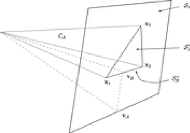
Figure 9: The geometry of the LARS–Stagewise modification.

Lemma 6.2.

The vector ${\bf v}_{\hat{\mathcal{B}}}$ satisfies Constraints I–III, and conversely if ${\bf v}$ satisfies the three constraints, then ${\bf v}={\bf v}_{\hat{\mathcal{B}}}$.

Let $\operatorname{Cos}\equiv A_{\mathcal{A}}/A_{\mathcal{B}}$ and $\operatorname{Sin}=[1-\mbox{Cos}^{2}]^{1/2}$, the latter being greater than zero by Lemma 5.2. For any face ${\mathcal{B}}\subset{\mathcal{A}}$, (128) implies

$${\bf u}_{\mathcal{A}}=\operatorname{Cos}\cdot{\bf u}_{\mathcal{B}}+\operatorname{Sin}\cdot{\bf z}_{\mathcal{B}},$$ (130)

where ${\bf z}_{\mathcal{B}}$ is a unit vector orthogonal to ${\mathcal{L}}(X_{\mathcal{B}})$, pointing away from ${\mathcal{C}}_{\mathcal{A}}$. By an $n$-dimensional coordinate rotation we can make ${\mathcal{L}}(X_{\mathcal{B}})={\mathcal{L}}({\bf c}_{1},{\bf c}_{2},\ldots,{\bf c}_{J})$, $J=|{\mathcal{B}}|$, the space of $n$-vectors with last $n-J$ coordinates zero, and also

$${\bf u}_{\mathcal{B}}=(1,{\bf 0},0,{\bf 0}),\qquad{\bf u}_{\mathcal{A}}=(\operatorname{Cos},{\bf 0},\operatorname{Sin},{\bf 0}),$$ (131)

the first ${\bf 0}$ having length $J-1$, the second 0 length $n-J-1$. Then we can write

$${\bf x}_{j}=\bigl{(}A_{\mathcal{B}},{\bf x}_{j_{2}},0,{\bf 0}\bigr{)}\qquad\mbox{for }j\in{\mathcal{B}},$$ (132)

the first coordinate $A_{\mathcal{B}}$ being required since ${\bf x}_{j}^{\prime}{\bf u}_{\mathcal{B}}=A_{\mathcal{B}}$, (14). Notice that ${\bf x}_{j}^{\prime}{\bf u}_{\mathcal{A}}=\operatorname{Cos}\cdot A_{\mathcal{B}}=A_{\mathcal{A}}$, as also required by (14).

For $\ell\in{\mathcal{A}}-{\mathcal{B}}$ denote ${\bf x}_{\ell}$ as

$${\bf x}_{\ell}=\bigl{(}x_{\ell_{1}},{\bf x}_{\ell_{2}},x_{\ell_{3}},{\bf x}_{\ell_{4}}\bigr{)},$$ (133)

so (14) yields

$$A_{\mathcal{A}}={\bf x}_{\ell}^{\prime}{\bf u}_{\mathcal{A}}=\operatorname{Cos}\cdot x_{\ell_{1}}+\operatorname{Sin}\cdot x_{\ell_{3}}.$$ (134)

Now assume ${\mathcal{B}}=\widehat{\mathcal{B}}$. In this case a separating hyperplane ${\mathcal{H}}$ orthogonal to ${\bf z}_{\hat{\mathcal{B}}}$ in (130) passes between the convex cone ${\mathcal{C}}_{\mathcal{A}}$ and ${\bf u}_{\mathcal{A}}$, through $\widehat{\bf u}_{\mathcal{A}}=\operatorname{Cos}\cdot{\bf u}_{\hat{\mathcal{B}}}$, implying $x_{\ell_{3}}\leq 0$ [i.e., ${\bf x}_{\ell}$ and ${\bf u}_{\mathcal{A}}$ are on opposite sides of ${\mathcal{H}}$, $x_{\ell_{3}}$ being negative since the corresponding coordinate of ${\bf u}_{\mathcal{A}}$, “Sin” in (131), is positive]. Equation (134) gives $\operatorname{Cos}\cdot x_{\ell_{1}}\geq A_{\mathcal{A}}=\operatorname{Cos}\cdot A_{\hat{\mathcal{B}}}$ or

$${\bf x}_{\ell}^{\prime}{\bf v}_{\hat{\mathcal{B}}}=x_{\ell}^{\prime}(A_{\hat{\mathcal{B}}}{\bf u}_{\hat{\mathcal{B}}})=A_{\hat{\mathcal{B}}}x_{\ell_{1}}\geq A_{\hat{\mathcal{B}}}^{2},$$ (135)

verifying that Constraint III is satisfied.

Conversely suppose that ${\bf v}$ satisfies Constraints I–III so that ${\bf v}\in{\mathcal{S}}_{\mathcal{A}}^{+}$ and ${\bf v}={\bf v}_{\mathcal{B}}$ for the nonzero coefficient set ${\mathcal{B}}$: ${\bf v}_{\mathcal{B}}=\Sigma_{\mathcal{B}}{\bf x}_{j}P_{j},P_{j}>0$. Let ${\mathcal{H}}$ be the hyperplane passing through $\mbox{Cos}\cdot{\bf u}_{\mathcal{B}}$ orthogonally to ${\bf z}_{\mathcal{B}}$, (128), (130). If ${\bf v}_{\mathcal{B}}\neq{\bf v}_{\hat{\mathcal{B}}}$, then at least one of the vectors ${\bf x}_{\ell}$, $\ell\in{\mathcal{A}}-{\mathcal{B}}$, must lie on the same side of ${\mathcal{H}}$ as ${\bf u}_{\mathcal{A}}$, so that $x_{\ell_{3}}>0$ (or else ${\mathcal{H}}$ would be a separating hyperplane between ${\bf u}_{\mathcal{A}}$ and ${\mathcal{C}}_{\mathcal{A}}$, and ${\bf v}_{\mathcal{B}}$ would be proportional to $\widehat{\bf u}_{\mathcal{A}}$, the nearest point to ${\bf u}_{\mathcal{A}}$ in ${\mathcal{C}}_{\mathcal{A}}$, implying ${\bf v}_{\mathcal{B}}={\bf v}_{\hat{\mathcal{B}}}$). Now (134) gives $\mbox{Cos}\cdot x_{\ell_{1}}<A_{\mathcal{A}}=\mbox{Cos}\cdot A_{\mathcal{B}}$, or

$${\bf x}_{\ell}^{\prime}{\bf v}_{\mathcal{B}}={\bf x}_{\ell}^{\prime}(A_{\mathcal{B}}{\bf u}_{\mathcal{B}})=A_{\mathcal{B}}x_{\ell_{1}}<A_{\mathcal{B}}^{2}.$$ (136)

This violates Constraint III, showing that ${\bf v}$ must equal ${\bf v}_{\hat{\mathcal{B}}}$.

Notice that the direction of advance $\widehat{\bf v}={\bf v}_{\hat{\mathcal{B}}}$ of the idealized Stagewise procedure is a function only of the current maximal set $\widehat{\mathcal{A}}=\{j\dvtx|\widehat{c}_{j}|=\widehat{C}\}$, say $\widehat{\bf v}=\phi(\widehat{\mathcal{A}}\,)$. In the language of (126),

$$\frac{d\widehat{\bolds}{\beta}(z)}{dz}=\phi(\widehat{\mathcal{A}}\,).$$ (137)

The LARS–Stagewise algorithm of Theorem 2 produces an evolving family of estimates $\widehat{\bolds}{\beta}$ that everywhere satisfies (137). This is true at every LARS–Stagewise breakpoint by the definition of the Stagewise modification. It is also true between breakpoints. Let $\widehat{\mathcal{A}}$ be the maximal set at the breakpoint, giving $\widehat{\bf v}={\bf v}_{\hat{\mathcal{B}}}=\phi(\widehat{\mathcal{A}})$. In the succeeding LARS–Stagewise interval $\widehat{\bolds{\mu}}(\gamma)=\widehat{\bolds{\mu}}+\gamma{\bf v}_{\hat{\mathcal{B}}}$, the maximal set is immediately reduced to $\widehat{\mathcal{B}}$, according to properties (125), (126) of ${\bf v}_{\hat{\mathcal{B}}}$, at which it stays during the entire interval. However, $\phi(\widehat{\mathcal{B}}\,)=\phi(\widehat{\mathcal{A}}\,)={\bf v}_{\hat{\mathcal{B}}}$ since ${\bf v}_{\hat{\mathcal{B}}}\in{\mathcal{C}}_{\hat{\mathcal{B}}}$, so the LARS–Stagewise procedure, which continues in the direction $\widehat{\bf v}$ until a new member is added to the active set, continues to obey the idealized Stagewise equation (137).

All of this shows that the LARS–Stagewise algorithm produces a legitimate version of the idealized Stagewise track. The converse of Lemma 6.2 says that there are no other versions, verifying Theorem 2.

The Stagewise procedure has its potential generality as an advantage over LARS and Lasso: it is easy to define forward Stagewise methods for a wide variety of nonlinear fitting problems, as in Hastie, Tibshirani and Friedman [(2001), Chapter 10, which begins with a Stagewise analysis of “boosting”]. Comparisons with LARS and Lasso within the linear model framework, as at the end of Section 31, help us better understand Stagewise methodology. This section’s results permit further comparisons.

Consider proceeding forward from $\widehat{\bolds{\mu}}$ along unit vector ${\bf u}$, $\widehat{\bolds{\mu}}(\gamma)=\widehat{\bolds{\mu}}+\gamma{\bf u}$, two interesting choices being the LARS direction ${\bf u}_{\hat{\mathcal{A}}}$ and the Stagewise direction $\widehat{\bolds{\mu}}_{\hat{\mathcal{B}}}$. For ${\bf u}\in{\mathcal{L}}(X_{\hat{\mathcal{A}}})$, the rate of change of $S(\gamma)=\|{\bf y}-\widehat{\bolds{\mu}}(\gamma)\|^{2}$ is

$$-\frac{\partial S(\gamma)}{\partial\gamma}\bigg{|}_{0}=2\widehat{C}\cdot\frac{{\bf u}_{\mathcal{A}}^{\prime}\cdot{\bf u}}{A_{\hat{\mathcal{A}}}},$$ (138)

(138) following quickly from (89). This shows that the LARS direction ${\bf u}_{\hat{\mathcal{A}}}$ maximizes the instantaneous decrease in $S$. The ratio

$$\frac{\partial S_{\rm Stage}(\gamma)}{\partial\gamma}\bigg{|}_{0}\,\Big{/}\,\frac{\partial S_{\rm LARS}(\gamma)}{\partial\gamma}\bigg{|}_{0}=\frac{A_{\hat{\mathcal{A}}}}{A_{\hat{\mathcal{B}}}},$$ (139)

equaling the quantity “Cos” in (134).

The comparison goes the other way for the maximum absolute correlation $\widehat{C}(\gamma)$. Proceeding as in (22),

$$-\frac{\partial\widehat{C}(\gamma)}{\partial\gamma}\bigg{|}_{0}=\min_{\hat{\mathcal{A}}}\{|x_{j}^{\prime}{\bf u}|\}.$$ (140)

The argument for Lemma 6.2, using Constraints II and III, shows that ${\bf u}_{\hat{\mathcal{B}}}$ maximizes (140) at $A_{\hat{\mathcal{B}}}$, and that

$$\frac{\partial\widehat{C}_{\rm LARS}(\gamma)}{\partial\gamma}\bigg{|}_{0}\,\Big{/}\,\frac{\partial\widehat{C}_{\rm Stage}(\gamma)}{\partial\gamma}\bigg{|}_{0}=\frac{A_{\hat{\mathcal{A}}}}{A_{\hat{\mathcal{B}}}}.$$ (141)

The original motivation for the Stagewise procedure was to minimize residual squared error within a framework of parsimonious forward search. However, (139) shows that Stagewise is less greedy than LARS in this regard, it being more accurate to describe Stagewise as striving to minimize the maximum absolute residual correlation.

7 Computations.

The entire sequence of steps in the LARS algorithm with $m<n$ variables requires $O(m^{3}+nm^{2})$ computations—the cost of a least squares fit on $m$ variables.

In detail, at the $k$th of $m$ steps, we compute $m-k$ inner products $c_{jk}$ of the nonactive ${\bf x}_{j}$ with the current residuals to identify the next active variable, and then invert the $k\times k$ matrix ${\mathcal{G}}_{k}=X_{k}^{\prime}X_{k}$ to find the next LARS direction. We do this by updating the Cholesky factorization $R_{k-1}$ of ${\mathcal{G}}_{k-1}$ found at the previous step [Golub and Van Loan (1983)]. At the final step $m$, we have computed the Cholesky $R=R_{m}$ for the full cross-product matrix, which is the dominant calculation for a least squares fit. Hence the LARS sequence can be seen as a Cholesky factorization with a guided ordering of the variables.

The computations can be reduced further by recognizing that the inner products above can be updated at each iteration using the cross-product matrix $X^{\prime}X$ and the current directions. For $m\gg n$, this strategy is counterproductive and is not used.

For the lasso modification, the computations are similar, except that occasionally one has to drop a variable, and hence downdate $R_{k}$ [costing at most $O(m^{2})$ operations per downdate]. For the stagewise modification of LARS, we need to check at each iteration that the components of $w$ are all positive. If not, one or more variables are dropped [using the inner loop of the NNLS algorithm described in Lawson and Hanson (1974)], again requiring downdating of $R_{k}$. With many correlated variables, the stagewise version can take many more steps than LARS because of frequent dropping and adding of variables, increasing the computations by a factor up to 5 or more in extreme cases.

The LARS algorithm (in any of the three states above) works gracefully for the case where there are many more variables than observations: $m\gg n$. In this case LARS terminates at the saturated least squares fit after $n-1$ variables have entered the active set [at a cost of $O(n^{3})$ operations]. (This number is $n-1$ rather than $n$, because the columns of $X$ have been mean centered, and hence it has row-rank $n-1$.) We make a few more remarks about the $m\gg n$ case in the lasso state:

1. The LARS algorithm continues to provide Lasso solutions along the way, and the final solution highlights the fact that a Lasso fit can have no more than $n-1$ (mean centered) variables with nonzero coefficients.

2. Although the model involves no more than $n-1$ variables at any time, the number of different variables ever to have entered the model during the entire sequence can be—and typically is—greater than $n-1$.

3. The model sequence, particularly near the saturated end, tends to be quite variable with respect to small changes in $\bf y$.

4. The estimation of $\sigma^{2}$ may have to depend on an auxiliary method such as nearest neighbors (since the final model is saturated). We have not investigated the accuracy of the simple approximation formula (61) for the case $m>n$.

Documented S-PLUS implementations of LARS and associated functions are available from www-stat.stanford.edu/$\sim$hastie/Papers/; the diabetes data also appears there.

8 Boosting procedures.

One motivation for studying the Forward Stagewise algorithm is its usefulness in adaptive fitting for data mining. In particular, Forward Stagewise ideas are used in “boosting,” an important class of fitting methods for data mining introduced by Freund and Schapire (1997). These methods are one of the hottest topics in the area of machine learning, and one of the most effective prediction methods in current use. Boosting can use any adaptive fitting procedure as its “base learner” (model fitter): trees are a popular choice, as implemented in CART [Breiman, Friedman, Olshen and Stone (1984)].

Friedman, Hastie and Tibshirani (2000) and Friedman (2001) studied boosting and proposed a number of procedures, the most relevant to this discussion being least squares boosting. This procedure works by successive fitting of regression trees to the current residuals. Specifically we start with the residual ${\bf r}={\bf y}$ and the fit $\hat{\bf y}=0$. We fit a tree in ${{\bf x}_{1},{\bf x}_{2},\ldots,{\bf x}_{m}}$ to the response ${\bf y}$ giving a fitted tree ${\bf t}_{1}$ (an $n$-vector of fitted values). Then we update $\hat{\bf y}$ to $\hat{\bf y}+\varepsilon\cdot{\bf t}_{1}$, ${\bf r}$ to ${\bf y}-\hat{\bf y}$ and continue for many iterations. Here $\varepsilon$ is a small positive constant. Empirical studies show that small values of $\varepsilon$ work better than $\varepsilon=1$: in fact, for prediction accuracy “the smaller the better.” The only drawback in taking very small values of $\varepsilon$ is computational slowness.

A major research question has been why boosting works so well, and specifically why is $\varepsilon$-shrinkage so important? To understand boosted trees in the present context, we think of our predictors not as our original variables ${{\bf x}_{1},{\bf x}_{2},\ldots,{\bf x}_{m}}$, but instead as the set of all trees ${\bf t}_{k}$ that could be fitted to our data. There is a strong similarity between least squares boosting and Forward Stagewise regression as defined earlier. Fitting a tree to the current residual is a numerical way of finding the “predictor” most correlated with the residual. Note, however, that the greedy algorithms used in CART do not search among all possible trees, but only a subset of them. In addition the set of all trees, including a parametrization for the predicted values in the terminal nodes, is infinite. Nevertheless one can define idealized versions of least-squares boosting that look much like Forward Stagewise regression.

Hastie, Tibshirani and Friedman (2001) noted the the striking similarity between Forward Stagewise regression and the Lasso, and conjectured that this may help explain the success of the Forward Stagewise process used in least squares boosting. That is, in some sense least squares boosting may be carrying out a Lasso fit on the infinite set of tree predictors. Note that direct computation of the Lasso via the LARS procedure would not be feasible in this setting because the number of trees is infinite and one could not compute the optimal step length. However, Forward Stagewise regression is feasible because it only need find the the most correlated predictor among the infinite set, where it approximates by numerical search.

In this paper we have established the connection between the Lasso and Forward Stagewise regression. We are now thinking about how these results can help to understand and improve boosting procedures. One such idea is a modified form of Forward Stagewise: we find the best tree as usual, but rather than taking a small step in only that tree, we take a small least squares step in all trees currently in our model. One can show that for small step sizes this procedure approximates LARS; its advantage is that it can be carried out on an infinite set of predictors such as trees.

*Appendix

Appendix A Local linearity and Lemma 4.2.

We write ${\bf x}_{l}$ with subscript $l$ for members of the active set ${\mathcal{A}}_{k}$. Thus ${\bf x}_{l}$ denotes the $l$th variable to enter, being an abuse of notation for $s_{l}{\bf x}_{j(l)}=\mbox{sgn}(\hat{c}_{j(l)}){\bf x}_{j(l)}$. Expressions ${\bf x}_{l}^{\prime}({\bf y}-\hat{\bolds{\mu}}_{k-1}({\bf y}))=\hat{C}_{k}({\bf y})$ and ${\bf x}_{l}^{\prime}{\bf u}_{k}=A_{k}$ clearly do not depend on which ${\bf x}_{l}\in{\mathcal{A}}_{k}$ we choose.

By writing $j\notin{\mathcal{A}}_{k}$, we intend that both ${\bf x}_{j}$ and $-{\bf x}_{j}$ are candidates for inclusion at the next step. One could think of negative indices $-j$ corresponding to “new” variables ${\bf x}_{-j}=-{\bf x}_{j}$.

The active set ${\mathcal{A}}_{k}({\bf y})$ depends on the data ${\bf y}$. When ${\mathcal{A}}_{k}({\bf y})$ is the same for all ${\bf y}$ in a neighborhood of ${\bf y}_{0}$, we say that ${\mathcal{A}}_{k}({\bf y})$ is locally fixed [at ${\mathcal{A}}_{k}={\mathcal{A}}_{k}({\bf y}_{0})$].

A function $g({\bf y})$ is locally Lipschitz at ${\bf y}$ if for all sufficiently small vectors $\Delta{\bf y}$,

$$\|\Delta g\|=\|g({\bf y}+\Delta{\bf y})-g({\bf y})\|\leq L\|\Delta{\bf y}\|.$$ (A.142)

If the constant $L$ applies for all ${\bf y}$, we say that $g$ is uniformly locally Lipschitz $(L)$, and the word “locally” may be dropped.

Lemma A.1.

For each $k$, $0\leq k\leq m$, there is an open set $G_{k}$ of full measure on which ${\mathcal{A}}_{k}({\bf y})$ and ${\mathcal{A}}_{k+1}({\bf y})$ are locally fixed and differ by $1$, and $\hat{\bolds{\mu}}_{k}({\bf y})$ is locally linear. The sets $G_{k}$ are decreasing as $k$ increases.

The argument is by induction. The induction hypothesis states that for each ${\bf y}_{0}\in G_{k-1}$ there is a small ball $B({\bf y}_{0})$ on which (a) the active sets ${\mathcal{A}}_{k-1}({\bf y})$ and ${\mathcal{A}}_{k}({\bf y})$ are fixed and equal to ${\mathcal{A}}_{k-1}$ and ${\mathcal{A}}_{k}$, respectively, (b) $|{\mathcal{A}}_{k}\setminus{\mathcal{A}}_{k-1}|=1$ so that the same single variable enters locally at stage $k-1$ and (c) $\hat{\bolds{\mu}}_{k-1}({\bf y})=M{\bf y}$ is linear. We construct a set $G_{k}$ with the same property.

Fix a point ${\bf y}_{0}$ and the corresponding ball $B({\bf y}_{0})\subset G_{k-1}$, on which ${\bf y}-\hat{\bolds{\mu}}_{k-1}({\bf y})={\bf y}-M{\bf y}=R{\bf y}$, say. For indices $j_{1},j_{2}\notin{\mathcal{A}}$, let $N(j_{1},j_{2})$ be the set of ${\bf y}$ for which there exists a $\gamma$ such that

$$w^{\prime}(R{\bf y}-\gamma{\bf u}_{k})={\bf x}_{j_{1}}^{\prime}(R{\bf y}-\gamma{\bf u}_{k})={\bf x}_{j_{2}}^{\prime}(R{\bf y}-\gamma{\bf u}_{k}).$$ (A.143)

Setting $\bolds{\delta}_{1}={\bf x}_{l}-{\bf x}_{j_{1}}$, the first equality may be written $\bolds{\delta}_{1}^{\prime}R{\bf y}=\gamma\bolds{\delta}_{1}^{\prime}{\bf u}_{k}$ and so when $\bolds{\delta}_{1}^{\prime}{\bf u}_{k}\neq 0$ determines

$$\gamma=\bolds{\delta}_{1}^{\prime}R{\bf y}/\bolds{\delta}_{1}^{\prime}{\bf u}_{k}=:{\bolds{\eta}}_{1}^{\prime}{\bf y}.$$

[If $\bolds{\delta}_{1}^{\prime}{\bf u}_{k}=0$, there are no qualifying ${\bf y}$, and $N(j_{1},j_{2})$ is empty.] Now using the second equality and setting $\bolds{\delta}_{2}={\bf x}_{l}-{\bf x}_{j_{2}}$, we see that $N(j_{1},j_{2})$ is contained in the set of ${\bf y}$ for which

$$\bolds{\delta}_{2}^{\prime}R{\bf y}=\eta_{1}^{\prime}{\bf y}\ \bolds{\delta}_{2}^{\prime}{\bf u}_{k}.$$

In other words, setting ${\bolds{\eta}}_{2}=R^{\prime}\bolds{\delta}_{2}-(\bolds{\delta}_{2}^{\prime}{\bf u}_{k}){\bolds{\eta}}_{1}$, we have

$$N(j_{1},j_{2})\subset\{{\bf y}\dvtx{\bolds{\eta}}_{2}^{\prime}{\bf y}=0\}.$$

If we define

$$N({\bf y}_{0})=\bigcup\{N(j_{1},j_{2})\dvtx j_{1},j_{2}\notin{\mathcal{A}},j_{1}\neq j_{2}\},$$

it is evident that $N({\bf y}_{0})$ is a finite union of hyperplanes and hence closed. For ${\bf y}\in B({\bf y}_{0})\setminus N({\bf y}_{0})$, a unique new variable joins the active set at step $k$. Near each such ${\bf y}$ the “joining” variable is locally the same and $\gamma_{k}({\bf y}){\bf u}_{k}$ is locally linear.

We then define $G_{k}\subset G_{k-1}$ as the union of such sets $B({\bf y})\setminus N({\bf y})$ over ${\bf y}\in G_{k-1}$. Thus $G_{k}$ is open and, on $G_{k}$, ${\mathcal{A}}_{k+1}({\bf y})$ is locally constant and $\hat{\bolds{\mu}}_{k}({\bf y})$ is locally linear. Thus properties (a)–(c) hold for $G_{k}$.

The same argument works for the initial case $k=0$: since $\hat{\bolds{\mu}}_{0}=0$, there is no circularity.

Finally, since the intersection of $G_{k}$ with any compact set is covered by a finite number of $B(y_{i})\setminus N(y_{i})$, it is clear that $G_{k}$ has full measure.

Lemma A.2.

Suppose that, for ${\bf y}$ near ${\bf y}_{0}$, $\hat{\bolds{\mu}}_{k-1}({\bf y})$ is continuous (resp. linear) and that ${\mathcal{A}}_{k}({\bf y})={\mathcal{A}}_{k}$. Suppose also that, at ${\bf y}_{0}$, ${\mathcal{A}}_{k+1}({\bf y}_{0})={\mathcal{A}}\cup\{k+1\}$.

Then for ${\bf y}$ near ${\bf y}_{0}$, ${\mathcal{A}}_{k+1}({\bf y})={\mathcal{A}}_{k}\cup\{k+1\}$ and $\hat{\gamma}_{k}({\bf y})$ and hence $\hat{\bolds{\mu}}_{k}({\bf y})$ are continuous (resp. linear) and uniformly Lipschitz.

Consider first the situation at ${\bf y}_{0}$, with $\widehat{C}_{k}$ and $\widehat{c}_{kj}$ defined in (25) and (24), respectively. Since $k+1\notin{\mathcal{A}}_{k}$, we have $|\hat{C}_{k}({\bf y}_{0})|>\hat{c}_{k,k+1}({\bf y}_{0})$, and $\hat{\gamma}_{k}({\bf y}_{0})>0$ satisfies

$$\qquad\hskip 3.0pt\hat{C}_{k}({\bf y}_{0})-\hat{\gamma}_{k}({\bf y}_{0})A_{k}\ \left\{\matrix{=\cr>}\right\}\ \hat{c}_{k,j}({\bf y}_{0})-\hat{\gamma}_{k}({\bf y}_{0})a_{k,j}\qquad\mbox{as }\left\{\matrix{j=k+1\cr j>k+1}.\right.$$ (A.144)

In particular, it must be that $A_{k}\neq a_{k,k+1}$, and hence

$$\hat{\gamma}_{k}({\bf y}_{0})=\frac{\hat{C}_{k}({\bf y}_{0})-\hat{c}_{k,k+1}({\bf y}_{0})}{A_{k}-a_{k,k+1}}>0.$$

Call an index $j$ admissible if $j\notin{\mathcal{A}}_{k}$ and $a_{k,j}\neq A_{k}$. For ${\bf y}$ near ${\bf y}_{0}$, this property is independent of ${\bf y}$. For admissible $j$, define

$$R_{k,j}({\bf y})=\frac{\hat{C}_{k}({\bf y})-\hat{c}_{k,j}({\bf y})}{A_{k}-a_{k,j}},$$

which is continuous (resp. linear) near ${\bf y}_{0}$ from the assumption on $\hat{\bolds{\mu}}_{k-1}.$ By definition,

$$\hat{\gamma}_{k}({\bf y})=\min_{j\in{\mathcal{P}}_{k}({\bf y})}R_{k,j}({\bf y}),$$

where

$${\mathcal{P}}_{k}({\bf y})=\{j\mbox{ admissible and }R_{k,j}({\bf y})>0\}.$$

For admissible $j$, $R_{k,j}({\bf y}_{0})\neq 0,$ and near ${\bf y}_{0}$ the functions ${\bf y}\rightarrow R_{k,j}({\bf y})$ are continuous and of fixed sign. Thus, near ${\bf y}_{0}$ the set ${\mathcal{P}}_{k}({\bf y})$ stays fixed at ${\mathcal{P}}_{k}({\bf y}_{0})$ and (A.144) implies that

$$R_{k,k+1}({\bf y})<R_{k,j}({\bf y}),\qquad j>k+1,j\in{\mathcal{P}}_{k}({\bf y}).$$

Consequently, for ${\bf y}$ near ${\bf y}_{0}$, only variable $k+1$ joins the active set, and so ${\mathcal{A}}_{k+1}({\bf y})={\mathcal{A}}_{k}\cup\{k+1\}$, and

$$\hat{\gamma}_{k}({\bf y})=R_{k,k+1}({\bf y})=\frac{({\bf x}_{l}-{\bf x}_{k+1})^{\prime}({\bf y}-\hat{\bolds{\mu}}_{k-1}({\bf y}))}{({\bf x}_{l}-{\bf x}_{k+1})^{\prime}{\bf u}_{k}}.$$ (A.145)

This representation shows that both $\hat{\gamma}_{k}({\bf y})$ and hence $\hat{\bolds{\mu}}_{k}({\bf y})=\hat{\bolds{\mu}}_{k-1}({\bf y})+\hat{\gamma}_{k}({\bf y}){\bf u}_{k}$ are continuous (resp. linear) near ${\bf y}_{0}$.

To show that $\hat{\gamma}_{k}$ is locally Lipschitz at ${\bf y}$, we set $\bolds{\delta}={\bf w}-{\bf x}_{k+1}$ and write, using notation from (A.142),

$$\Delta\hat{\gamma}_{k}=\frac{\bolds{\delta}^{\prime}(\Delta{\bf y}-\Delta\hat{\bolds{\mu}}_{k-1})}{\bolds{\delta}^{\prime}{\bf u}_{k}}.$$

As ${\bf y}$ varies, there is a finite list of vectors $({\bf x}_{l},{\bf x}_{k+1},{\bf u}_{k})$ that can occur in the denominator term $\bolds{\delta}^{\prime}{\bf u}_{k}$, and since all such terms are positive [as observed below (A.144)], they have a uniform positive lower bound, $a_{\min}$ say. Since $\|\bolds{\delta}\|\leq 2$ and $\hat{\bolds{\mu}}_{k-1}$ is Lipschitz $(L_{k-1})$ by assumption, we conclude that

$$\frac{|\Delta\hat{\gamma}_{k}|}{\|\Delta{\bf y}\|}\leq 2a_{\min}^{-1}(1+L_{k-1})=:L_{k}.$$

Appendix B Consequences of the positive cone condition.

Lemma B.1.

Suppose that $|{\mathcal{A}}_{+}|=|{\mathcal{A}}|+1$ and that $X_{{\mathcal{A}}+}=[X_{{\mathcal{A}}}\ \ {\bf x}_{+}]$ (where ${\bf x}_{+}=s_{j}{\bf x}_{j}$ for some $j\notin{\mathcal{A}}$). Let $P_{\mathcal{A}}=X_{\mathcal{A}}G_{\mathcal{A}}^{-1}X_{\mathcal{A}}^{\prime}$ denote projection on ${\rm span}(X_{\mathcal{A}}),$ so that $a={\bf x}_{+}^{\prime}P_{\mathcal{A}}{\bf x}_{+}<1.$ The $+$-component of $G_{{\mathcal{A}}+}^{-1}{\bf 1}_{{\mathcal{A}}+}$ is

$$(G_{{\mathcal{A}}+}^{-1}{\bf 1}_{{\mathcal{A}}+})_{+}=(1-a)^{-1}\biggl{(}1-\frac{{\bf x}_{+}^{\prime}{\bf u}_{\mathcal{A}}}{A_{\mathcal{A}}}\biggr{)}.$$ (B.146)

Consequently, under the positive cone condition (60),

$${\bf x}_{+}^{\prime}{\bf u}_{\mathcal{A}}<A_{\mathcal{A}}.$$ (B.147)

Write $G_{{\mathcal{A}}+}$ as a partitioned matrix

$$G_{{\mathcal{A}}+}=\pmatrix{X^{\prime}X&X^{\prime}{\bf x}_{+}\cr{\bf x}_{+}^{\prime}X&{\bf x}_{+}^{\prime}{\bf x}_{+}}=\pmatrix{A&B\cr B^{\prime}&D}.$$

Applying the formula for the inverse of a partitioned matrix [e.g., Rao (1973), page 33],

$$(G_{{\mathcal{A}}+}^{-1}{\bf 1}_{{\mathcal{A}}+})_{+}=-E^{-1}F^{\prime}{\bf 1}+E^{-1},$$

where

$$E = D-B^{\prime}A^{-1}B=1-{\bf x}_{+}^{\prime}P_{\mathcal{A}}{\bf x}_{+},$$

$$F = A^{-1}B=G_{\mathcal{A}}^{-1}X^{\prime}{\bf x}_{+},$$

from which (B.146) follows. The positive cone condition implies that $G_{{\mathcal{A}}+}^{-1}{\bf 1}_{{\mathcal{A}}+}>0$, and so (B.147) is immediate.

Appendix C Global continuity and Lemma 4.3.

We shall call ${\bf y}_{0}$ a multiple point at step $k$ if two or more variables enter at the same time. Lemma A.2 shows that such points form a set of measure zero, but they can and do cause discontinuities in $\hat{\bolds{\mu}}_{k+1}$ at ${\bf y}_{0}$ in general. We will see, however, that the positive cone condition prevents such discontinuities.

We confine our discussion to double points, hoping that these arguments will be sufficient to establish the same pattern of behavior at points of multiplicity 3 or higher. In addition, by renumbering, we shall suppose that indices $k+1$ and $k+2$ are those that are added at double point ${\bf y}_{0}$. Similarly, for convenience only, we assume that ${\mathcal{A}}_{k}({\bf y})$ is constant near ${\bf y}_{0}$. Our task then is to show that, for ${\bf y}$ near a double point ${\bf y}_{0}$, both $\hat{\bolds{\mu}}_{k}({\bf y})$ and $\hat{\bolds{\mu}}_{k+1}({\bf y})$ are continuous and uniformly locally Lipschitz.

Lemma C.1.

Suppose that ${\mathcal{A}}_{k}({\bf y})={\mathcal{A}}_{k}$ is constant near ${\bf y}_{0}$ and that ${\mathcal{A}}_{k+}({\bf y}_{0})={\mathcal{A}}_{k}\cup\{k+1,k+2\}$. Then for ${\bf y}$ near ${\bf y}_{0}$, ${\mathcal{A}}_{k+}({\bf y})\setminus{\mathcal{A}}_{k}$ can only be one of three possibilities, namely $\{k+1\},\{k+2\}$ or $\{k+1,k+2\}$. In all cases $\hat{\bolds{\mu}}_{k}({\bf y})=\hat{\bolds{\mu}}_{k-1}({\bf y})+\hat{\gamma}_{k}({\bf y}){\bf u}_{k}$ as usual, and both $\gamma_{k}({\bf y})$ and $\hat{\bolds{\mu}}_{k}({\bf y})$ are continuous and locally Lipschitz.

We use notation and tools from the proof of Lemma A.2. Since ${\bf y}_{0}$ is a double point and the positivity set ${\mathcal{P}}_{k}({\bf y})={\mathcal{P}}_{k}$ near ${\bf y}_{0}$, we have

$$0<R_{k,k+1}({\bf y}_{0})=R_{k,k+2}({\bf y}_{0})<R_{k,j}({\bf y}_{0})\qquad\mbox{for }j\in{\mathcal{P}}_{k}\setminus\{k+1,k+2\}.$$

Continuity of $R_{k,j}$ implies that near ${\bf y}_{0}$ we still have

$$0<R_{k,k+1}({\bf y}),R_{k,k+2}({\bf y})<\min\bigl{\{}R_{k,j}({\bf y});j\in{\mathcal{P}}_{k}\setminus\{k+1,k+2\}\bigr{\}}.$$

Hence ${\mathcal{A}}_{k+}\setminus{\mathcal{A}}_{k}$ must equal $\{k+1\}$ or $\{k+2\}$ or $\{k+1,k+2\}$ according as $R_{k,k+1}({\bf y})$ is less than, greater than or equal to $R_{k,k+2}({\bf y}).$ The continuity of

$$\hat{\gamma}_{k}({\bf y})=\min\{R_{k,k+1}({\bf y}),R_{k,k+2}({\bf y})\}$$

is immediate, and the local Lipschitz property follows from the arguments of Lemma A.2.

Lemma C.2.

Assume the conditions of Lemma C.1 and in addition that the positive cone condition (60) holds. Then $\hat{\bolds{\mu}}_{k+1}({\bf y})$ is continuous and locally Lipschitz near ${\bf y}_{0}$.

Since ${\bf y}_{0}$ is a double point, property (A.144) holds, but now with equality when $j=k+1$ or $k+2$ and strict inequality otherwise. In other words, there exists $\delta_{0}>0$ for which

$$\hat{C}_{k+1}({\bf y}_{0})-\hat{c}_{k+1,j}({\bf y}_{0})\cases{=0,&\quad\mbox{if }$j=k+2$,\cr\geq\delta_{0},&\quad\mbox{if }$j>k+2$.}$$

Consider a neighborhood $B({\bf y}_{0})$ of ${\bf y}_{0}$ and let $N({\bf y}_{0})$ be the set of double points in $B({\bf y}_{0})$, that is, those for which ${\mathcal{A}}_{k+1}({\bf y})\setminus{\mathcal{A}}_{k}=\{k+1,k+2\}$. We establish the convention that at such double points $\hat{\bolds{\mu}}_{k+1}({\bf y})=\hat{\bolds{\mu}}_{k}({\bf y})$; at other points ${\bf y}$ in $B({\bf y}_{0})$, $\hat{\bolds{\mu}}_{k+1}({\bf y})$ is defined by $\hat{\bolds{\mu}}_{k}({\bf y})+\hat{\gamma}_{k+1}({\bf y}){\bf u}_{k+1}$ as usual.

Now consider those ${\bf y}$ near ${\bf y}_{0}$ for which ${\mathcal{A}}_{k+1}({\bf y})\setminus{\mathcal{A}}_{k}=\{k+1\}$, and so, from the previous lemma, ${\mathcal{A}}_{k+2}({\bf y})\setminus{\mathcal{A}}_{k+1}=\{k+2\}.$ For such ${\bf y}$, continuity and the local Lipschitz property for $\hat{\bolds{\mu}}_{k}$ imply that

$$\hat{C}_{k+1}({\bf y})-\hat{c}_{k+1,j}({\bf y})\cases{=O(\|{\bf y}-{\bf y}_{0}\|),&\quad\mbox{if } $j=k+2$,\cr>\delta_{0}/2,&\quad\mbox{if } $j>k+2$.}$$

It is at this point that we use the positive cone condition (via Lemma B.1) to guarantee that $A_{k+1}>a_{k+1,k+2}.$ Also, since ${\mathcal{A}}_{k+1}({\bf y})\setminus{\mathcal{A}}_{k}=\{k+1\}$, we have

$$\hat{C}_{k+1}({\bf y})>\hat{c}_{k+1,k+2}({\bf y}).$$

These two facts together show that $k+2\in{\mathcal{P}}_{k+1}({\bf y})$ and hence that

$$\hat{\gamma}_{k+1}({\bf y})=\frac{\hat{C}_{k+1}({\bf y})-\hat{c}_{k+1,k+2}({\bf y})}{A_{k+1}-a_{k+1,k+2}}=O(\|{\bf y}-{\bf y}_{0}\|)$$

is continuous and locally Lipschitz. In particular, as ${\bf y}$ approaches $N({\bf y}_{0})$, we have $\hat{\gamma}_{k+1}({\bf y})\rightarrow 0$.

Remark 5.

We say that a function $g\dvtx\mathbb{R}^{n}\rightarrow\mathbb{R}$ is almost differentiable if it is absolutely continuous on almost all line segments parallel to the coordinate axes, and its partial derivatives (which consequently exist a.e.) are locally integrable. This definition of almost differentiability appears superficially to be weaker than that given by Stein, but it is in fact precisely the property used in his proof. Furthermore, this definition is equivalent to the standard definition of weak differentiability used in analysis.

Proof of Lemma 4.3 We have shown explicitly that $\hat{\bolds{\mu}}_{k}({\bf y})$ is continuous and uniformly locally Lipschitz near single and double points. Similar arguments extend the property to points of multiplicity 3 and higher, and so all points ${\bf y}$ are covered. Finally, absolute continuity of ${\bf y}\rightarrow\hat{\bolds{\mu}}_{k}({\bf y})$ on line segments is a simple consequence of the uniform Lipschitz property, and so $\hat{\bolds{\mu}}_{k}$ is almost differentiable.

References

- Breiman, Friedman, Olshen and Stone (1984) Breiman, L., Friedman, J., Olshen, R. and Stone, C. (1984). Classification and Regression Trees. Wadsworth, Belmont, CA. \MR726392
- Efron (1986) Efron, B. (1986). How biased is the apparent error rate of a prediction rule? J. Amer. Statist. Assoc. 81 461–470. \MR845884
- Efron and Tibshirani (1997) Efron, B. and Tibshirani, R. (1997). Improvements on cross-validation: The bootstrap method. J. Amer. Statist. Assoc. 92 548–560. \MR1467848
- Freund and Schapire (1997) Freund, Y. and Schapire, R. (1997). A decision-theoretic generalization of online learning and an application to boosting. J. Comput. System Sci. 55 119–139. \MR1473055
- Friedman (2001) Friedman, J. (2001). Greedy function approximation: A gradient boosting machine. Ann. Statist. 29 1189–1232. \MR1873328