Isometric immersions into $\mathbb{S}^{n}\times\mathbb{R}$ and $\mathbb{H}^{n}\times\mathbb{R}$
and applications to minimal surfaces

Abstract.

We give a necessary and sufficient condition for an $n$-dimensional Riemannian manifold to be isometrically immersed in $\mathbb{S}^{n}\times\mathbb{R}$ or $\mathbb{H}^{n}\times\mathbb{R}$ in terms of its first and second fundamental forms and of the projection of the vertical vector field on its tangent plane. We deduce the existence of a one-parameter family of isometric minimal deformations of a given minimal surface in $\mathbb{S}^{2}\times\mathbb{R}$ or $\mathbb{H}^{2}\times\mathbb{R}$, obtained by rotating the shape operator.

1. Introduction

It is well known that the first and second fundamental forms of a hypersurface of a Riemannian manifold satisfy two compatibility equations called the Gauss and Codazzi equations. More precisely, let $\bar{\mathcal{V}}$ be an orientable Riemannian manifold of dimension $n+1$ and ${\mathcal{V}}$ a submanifold of $\bar{\mathcal{V}}$ of dimension $n$. Let $\nabla$ (respectively, $\bar{\nabla}$) be the Riemannian connection of ${\mathcal{V}}$ (respectively, $\bar{\mathcal{V}}$), $\mathrm{R}$ (respectively, $\bar{\mathrm{R}}$) the Riemann curvature tensor of ${\mathcal{V}}$ (respectively, $\bar{\mathcal{V}}$), i.e.,

$$\mathrm{R}(X,Y)Z=\nabla_{Y}\nabla_{X}Z-\nabla_{X}\nabla_{Y}Z+\nabla_{[X,Y]}Z,$$

and $\mathrm{S}$ the shape operator of ${\mathcal{V}}$ associated to its unit normal $N$, i.e., $\mathrm{S}X=-\bar{\nabla}_{X}N$. Then the following equations hold for all vector fields $X,Y,Z$ on ${\mathcal{V}}$:

$$\mathrm{R}(X,Y)Z-\bar{\mathrm{R}}(X,Y)Z=\langle\mathrm{S}X,Z\rangle\mathrm{S}Y-\langle\mathrm{S}Y,Z\rangle\mathrm{S}X,$$

$$\nabla_{X}\mathrm{S}Y-\nabla_{Y}\mathrm{S}X-\mathrm{S}[X,Y]=\bar{\mathrm{R}}(X,Y)N.$$

These are respectively the Gauss and Codazzi equations.

In the case where $\bar{\mathcal{V}}$ is a space form, i.e., the sphere $\mathbb{S}^{n+1}$, the Euclidean space $\mathbb{R}^{n+1}$ or the hyperbolic space $\mathbb{H}^{n+1}$, these equations become the following:

(1) $$\begin{array}[]{c}\langle\mathrm{R}(X,Y)Z,W\rangle-\kappa(\langle X,Z\rangle\langle Y,W\rangle-\langle Y,Z\rangle\langle X,W\rangle)\\ =\langle\mathrm{S}X,Z\rangle\langle\mathrm{S}Y,W\rangle-\langle\mathrm{S}X,W\rangle\langle\mathrm{S}Y,Z\rangle,\end{array}$$

(2) $$\nabla_{X}\mathrm{S}Y-\nabla_{Y}\mathrm{S}X-\mathrm{S}[X,Y]=0,$$

where $\kappa$ is the sectional curvature of $\bar{\mathcal{V}}$, i.e., $\kappa=1,0,-1$ for $\mathbb{S}^{n+1}$, $\mathbb{R}^{n+1}$ and $\mathbb{H}^{n+1}$ respectively. Thus the Gauss and Codazzi equations only involve the first and second fundamental forms of ${\mathcal{V}}$; they are defined intrinsicly on ${\mathcal{V}}$ (as soon as we know $\mathrm{S}$). This comes from the fact that these ambiant spaces are isotropic. Moreover, in this case the Gauss and Codazzi equations are also sufficient conditions for an $n$-dimensional simply connected manifold to be immersed into $\bar{\mathcal{V}}$ with given first and second fundamental forms: if ${\mathcal{V}}$ is a Riemannian manifold endowed with a field $\mathrm{S}$ of symmetric operators $\mathrm{S}_{y}:\mathrm{T}_{y}{\mathcal{V}}\to\mathrm{T}_{y}{\mathcal{V}}$ such that (1) and (2) hold (where $\mathrm{R}$ denotes the Riemann curvature tensor of ${\mathcal{V}}$), then there exists an isometric immersion from ${\mathcal{V}}$ into $\bar{\mathcal{V}}$ with $\mathrm{S}$ as shape operator. The reader can refer to [Car92], and also to [Ten71] for a proof in the case of $\mathbb{R}^{n+1}$.

In the case of a general manifold $\bar{\mathcal{V}}$, the Gauss and Codazzi equations are not defined intrinsicly on ${\mathcal{V}}$, since the Riemann curvature tensor of the ambiant space $\bar{\mathcal{V}}$ is involved. Yet, in the case where $\bar{\mathcal{V}}=\mathbb{S}^{n}\times\mathbb{R}$ or $\bar{\mathcal{V}}=\mathbb{H}^{n}\times\mathbb{R}$, these equations are well defined as soon as we know:

1. the projection $T$ of the vertical vector $\frac{\partial}{\partial t}$ (corresponding to the factor $\mathbb{R}$) onto the tangent space of ${\mathcal{V}}$,

2. the normal component $\nu$ of $\frac{\partial}{\partial t}$, i.e., $\nu=\langle N,\frac{\partial}{\partial t}\rangle$.

Indeed, the Gauss and Codazzi equations become the following:

$$\begin{array}[]{lll}\mathrm{R}(X,Y)Z&=&\langle\mathrm{S}X,Z\rangle\mathrm{S}Y-\langle\mathrm{S}Y,Z\rangle\mathrm{S}X\\ &&+\kappa(\langle X,Z\rangle Y-\langle Y,Z\rangle X-\langle Y,T\rangle\langle X,Z\rangle T\\ &&-\langle X,T\rangle\langle Z,T\rangle Y+\langle X,T\rangle\langle Y,Z\rangle T+\langle Y,T\rangle\langle Z,T\rangle X),\end{array}$$

$$\nabla_{X}\mathrm{S}Y-\nabla_{Y}\mathrm{S}X-\mathrm{S}[X,Y]=\kappa\nu(\langle Y,T\rangle X-\langle X,T\rangle Y),$$

where $\kappa=1$ and $\kappa=-1$ for $\mathbb{S}^{n}\times\mathbb{R}$ and $\mathbb{H}^{n}\times\mathbb{R}$ respectively.

The Gauss equation can be formulated in the following equivalent way: the sectional curvature $K(P)$ (for the metric of ${\mathcal{V}}$) of every plane $P\subset\mathrm{T}{\mathcal{V}}$ satisfies

$$K(P)=\det\mathrm{S}_{P}+\kappa(1-||T_{P}||^{2})$$

where $\mathrm{S}_{P}$ is the restriction of $\mathrm{S}$ on $P$ and $T_{P}$ the orthogonal projection of $T$ on $P$.

The first aim of this paper is to give a necessary and sufficient condition in order that a Riemannian manifold with a symmetric operator $\mathrm{S}$ can be isometrically immersed into $\mathbb{S}^{n}\times\mathbb{R}$ or $\mathbb{H}^{n}\times\mathbb{R}$ with $\mathrm{S}$ as shape operator. More precisely, we prove the following theorem.

Theorem (theorem 3.3).

Let ${\mathcal{V}}$ be a simply connected Riemannian manifold of dimension $n$, $\mathrm{d}s^{2}$ its metric (which we also denote by $\langle\cdot,\cdot\rangle$) and $\nabla$ its Riemannian connection. Let $\mathrm{S}$ be a field of symmetric operators $\mathrm{S}_{y}:\mathrm{T}_{y}{\mathcal{V}}\to\mathrm{T}_{y}{\mathcal{V}}$, $T$ a vector field on ${\mathcal{V}}$ and $\nu$ a smooth function on ${\mathcal{V}}$ such that $||T||^{2}+\nu^{2}=1$.

Let $\mathbb{M}^{n}=\mathbb{S}^{n}$ or $\mathbb{M}^{n}=\mathbb{H}^{n}$. Assume that $(\mathrm{d}s^{2},\mathrm{S},T,\nu)$ satisfies the Gauss and Codazzi equations for $\mathbb{M}^{n}\times\mathbb{R}$ and the following equations:

$$\nabla_{X}T=\nu\mathrm{S}X,\quad\mathrm{d}\nu(X)=-\langle\mathrm{S}X,T\rangle.$$

Then there exists an isometric immersion $f:{\mathcal{V}}\to\mathbb{M}^{n}\times\mathbb{R}$ such that the shape operator with respect to the normal $N$ associated to $f$ is

$$\mathrm{d}f\circ\mathrm{S}\circ\mathrm{d}f^{-1}$$

and such that

$$\frac{\partial}{\partial t}=\mathrm{d}f(T)+\nu N.$$

Moreover the immersion is unique up to a global isometry of $\mathbb{M}^{n}\times\mathbb{R}$ preserving the orientations of both $\mathbb{M}^{n}$ and $\mathbb{R}$.

The two additional conditions come from the fact that the vertical vector field $\frac{\partial}{\partial t}$ is parallel.

The method to prove this theorem is similar to that of Tenenblat ([Ten71]): it is based on differential forms, moving frames and integrable distributions.

This work was motivated by the study of minimal surfaces in $\mathbb{S}^{2}\times\mathbb{R}$ and $\mathbb{H}^{2}\times\mathbb{R}$. There were many recent developments in the theory of these surfaces. Rosenberg ([Ros02b]) studied the geometry of minimal surfaces in $\mathbb{S}^{2}\times\mathbb{R}$, and more generally in $M\times\mathbb{R}$ where $M$ is a surface of non-negative curvature. Nelli and Rosenberg ([NR02]) studied minimal surfaces in $\mathbb{H}^{2}\times\mathbb{R}$ and proved a Jenkins-Serrin theorem. Hauswirth ([Hau03]) constructed many examples in $\mathbb{H}^{2}\times\mathbb{R}$. Meeks and Rosenberg ([MR03]) initiated the theory of minimal surfaces in $M\times\mathbb{R}$ where $M$ is a compact surface. Recently, Abresch and Rosenberg ([AR03]) extended the notion of holomorphic Hopf differential to constant mean curvature surfaces in $\mathbb{S}^{2}\times\mathbb{R}$ and $\mathbb{H}^{2}\times\mathbb{R}$; using this holomorphic differential, they proved that all immersed constant mean curvature spheres are embedded and rotational.

In this paper, we use our theorem 3.3 to prove the existence of a one-parameter family of isometric minimal deformations of a given minimal surface in $\mathbb{S}^{2}\times\mathbb{R}$ or $\mathbb{H}^{2}\times\mathbb{R}$. This family is obtained by rotating the shape operator; hence it is the analog of the associate family of a minimal surface in $\mathbb{R}^{3}$. This is the following theorem.

Theorem (theorem 4.2).

Let $\Sigma$ be a simply connected Riemann surface and $x:\Sigma\to\mathbb{M}^{2}\times\mathbb{R}$ a conformal minimal immersion. Let $N$ be the induced normal. Let $\mathrm{S}$ be the symmetric operator on $\Sigma$ induced by the shape operator of $x(\Sigma)$. Let $T$ be the vector field on $\Sigma$ such that $\mathrm{d}x(T)$ is the projection of $\frac{\partial}{\partial t}$ onto $\mathrm{T}(x(\Sigma))$. Let $\nu=\left\langle N,\frac{\partial}{\partial t}\right\rangle$.

Let $z_{0}\in\Sigma$. Then there exists a unique family $(x_{\theta})_{\theta\in\mathbb{R}}$ of conformal minimal immersions $x_{\theta}:\Sigma\to\mathbb{M}^{2}\times\mathbb{R}$ such that:

1. $x_{\theta}(z_{0})=x(z_{0})$ and $(\mathrm{d}x_{\theta})_{z_{0}}=(\mathrm{d}x)_{z_{0}}$,

2. the metrics induced on $\Sigma$ by $x$ and $x_{\theta}$ are the same,

3. the symmetric operator on $\Sigma$ induced by the shape operator of $x_{\theta}(\Sigma)$ is $e^{\theta\mathrm{J}}\mathrm{S}$,

4. $\frac{\partial}{\partial t}=\mathrm{d}x_{\theta}(e^{\theta\mathrm{J}}T)+\nu N_{\theta}$ where $N_{\theta}$ is the unit normal to $x_{\theta}$.

Moreover we have $x_{0}=x$ and the family $(x_{\theta})$ is continuous with respect to $\theta$.

In particular taking $\theta=\frac{\pi}{2}$ defines a conjugate surface; the geometric properties of conjugate surfaces in $\mathbb{M}^{2}\times\mathbb{R}$ and in $\mathbb{R}^{3}$ are similar. Finally, we give examples of conjugate surfaces. In $\mathbb{S}^{2}\times\mathbb{R}$, we show that helicoids and unduloids are conjugate. In $\mathbb{H}^{2}\times\mathbb{R}$, we show that helicoids are conjugated to catenoids or to minimal surfaces foliated by horizontal curves of constant curvature belonging to the Hauswirth family (see [Hau03]).

2. Preliminaries

Notations.

In this paper we will use the following index conventions: Latin letters $i$, $j$, etc, denote integers between $1$ and $n$, Greek letters $\alpha$, $\beta$, etc, denote integers between $0$ and $n+1$. For example, the notation $A^{i}_{j}=B^{i}_{j}$ means that this relation holds for all integers $i$, $j$ between $1$ and $n$, the notation $\sum_{\alpha}C_{\alpha}$ means $C_{0}+C_{1}+\dots+C_{n+1}$.

The set of vector fields on a Riemannian manifold ${\mathcal{V}}$ will be denoted by $\mathfrak{X}({\mathcal{V}})$.

We denote by $\frac{\partial}{\partial t}$ the unit vector giving the orientation of $\mathbb{R}$ in $\mathbb{M}^{n}\times\mathbb{R}$; we call it the vertical vector.

2.1. The compatibility equations in $\mathbb{M}^{n}\times\mathbb{R}$

Let $\mathbb{M}^{n}=\mathbb{S}^{n}$ or $\mathbb{M}^{n}=\mathbb{H}^{n}$; in the first case we set $\kappa=1$ and in the second case we set $\kappa=-1$. Let $\bar{\mathrm{R}}$ be the Riemann curvature tensor of $\mathbb{M}^{n}\times\mathbb{R}$. Let ${\mathcal{V}}$ be an oriented hypersurface of $\mathbb{M}^{n}\times\mathbb{R}$ and $N$ the unit normal to ${\mathcal{V}}$.

Proposition 2.1.

For $X,Y,Z,W\in\mathfrak{X}({\mathcal{V}})$ we have

$$\langle\bar{\mathrm{R}}(X,Y)Z,W\rangle = \kappa(\langle X,Z\rangle\langle Y,W\rangle-\langle Y,Z\rangle\langle X,W\rangle$$

$$-\langle Y,T\rangle\langle W,T\rangle\langle X,Z\rangle-\langle X,T\rangle\langle Z,T\rangle\langle Y,W\rangle$$

$$+\langle X,T\rangle\langle W,T\rangle\langle Y,Z\rangle+\langle Y,T\rangle\langle Z,T\rangle\langle X,W\rangle),$$

$$\langle\bar{\mathrm{R}}(X,Y)N,Z\rangle=\kappa\nu(\langle X,Z\rangle\langle Y,T\rangle-\langle Y,Z\rangle\langle X,T\rangle),$$

where

$$\nu=\left\langle N,\frac{\partial}{\partial t}\right\rangle$$

and $T$ is the projection of $\frac{\partial}{\partial t}$ on $\mathrm{T}{\mathcal{V}}$, i.e.,

$$T=\frac{\partial}{\partial t}-\nu N.$$

Proof.

Any vector field on $\mathbb{M}^{n}\times\mathbb{R}$ can be written $X(m,t)=(X_{\mathbb{M}^{n}}^{t}(m),X_{\mathbb{R}}^{m}(t))$ where, for each $t\in\mathbb{R}$, $X_{\mathbb{M}^{n}}^{t}$ is a vector field on $\mathbb{M}^{n}$, and, for each $m\in\mathbb{M}^{n}$, $X_{\mathbb{R}}^{m}$ is a vector field on $\mathbb{R}$. Then for $X,Y,Z,W\in\mathfrak{X}(\mathbb{M}^{n}\times\mathbb{R})$ we have

$$\langle\bar{\mathrm{R}}(X,Y)Z,W\rangle = \langle\bar{\mathrm{R}}_{\mathbb{M}^{n}}(X_{\mathbb{M}^{n}},Y_{\mathbb{M}^{n}})Z_{\mathbb{M}^{n}},W_{\mathbb{M}^{n}}\rangle$$

$$= \kappa(\langle X_{\mathbb{M}^{n}},Z_{\mathbb{M}^{n}}\rangle\langle Y_{\mathbb{M}^{n}},W_{\mathbb{M}^{n}}\rangle-\langle Y_{\mathbb{M}^{n}},Z_{\mathbb{M}^{n}}\rangle\langle X_{\mathbb{M}^{n}},W_{\mathbb{M}^{n}}\rangle).$$

We have $X_{\mathbb{M}^{n}}=X-\left\langle X,\frac{\partial}{\partial t}\right\rangle\frac{\partial}{\partial t}$. Thus, if $X\in\mathrm{T}{\mathcal{V}}$, we have $X_{\mathbb{M}^{n}}=X-\langle X,T\rangle\frac{\partial}{\partial t}$, and similar expressions for $Y,Z,W\in\mathrm{T}{\mathcal{V}}$. A computation gives the expected formula for $\langle\bar{\mathrm{R}}(X,Y)Z,W\rangle$.

Finally we have $N_{\mathbb{M}^{n}}=N-\nu\frac{\partial}{\partial t}$, so a computation gives the expected formula for $\langle\bar{\mathrm{R}}(X,Y)N,Z\rangle$. ∎

Using the fact that the vector field $\frac{\partial}{\partial t}$ is parallel, we obtain the following equations.

Proposition 2.2.

For $X\in\mathfrak{X}({\mathcal{V}})$ we have

$$\nabla_{X}T=\nu\mathrm{S}X,\quad\mathrm{d}\nu(X)=-\langle\mathrm{S}X,T\rangle.$$

Proof.

We have $\frac{\partial}{\partial t}=T+\nu N$ and $\bar{\nabla}_{X}\frac{\partial}{\partial t}=0$. Thus we get

$$0=\bar{\nabla}_{X}T+(\mathrm{d}\nu(X))N+\nu\bar{\nabla}_{X}N=\nabla_{X}T+\langle\mathrm{S}X,T\rangle N+(\mathrm{d}\nu(X))N-\nu\mathrm{S}X.$$

Taking the tangential and the normal components in this equality, we obtain the expected formulas. ∎

Remark 2.3.

In the case of an orthonormal pair $(X,Y)$ we get

$$\langle\bar{\mathrm{R}}(X,Y)X,Y\rangle=\kappa(1-\langle Y,T\rangle^{2}-\langle X,T\rangle^{2}).$$

The reader can also refer to section 3.2 in [AR03].

2.2. Moving frames

In this section we introduce some material about the technique of moving frames. The reader can also refer to [Ros02a].

Let ${\mathcal{V}}$ be a Riemannian manifold of dimension $n$, $\nabla$ its Levi-Civita connection, and $\mathrm{R}$ the Riemannian curvature tensor. Let $\mathrm{S}$ be a field of symmetric operators $\mathrm{S}_{y}:\mathrm{T}_{y}{\mathcal{V}}\to\mathrm{T}_{y}{\mathcal{V}}$. Let $(e_{1},\dots,e_{n})$ be a local orthonormal frame on ${\mathcal{V}}$ and $(\omega^{1},\dots,\omega^{n})$ the dual basis of $(e_{1},\dots,e_{n})$, i.e.,

$$\omega^{i}(e_{k})=\delta^{i}_{k}.$$

We also set

$$\omega^{n+1}=0.$$

We define the forms $\omega^{i}_{j}$, $\omega^{n+1}_{j}$, $\omega^{i}_{n+1}$ and $\omega^{n+1}_{n+1}$ on ${\mathcal{V}}$ by

$$\omega^{i}_{j}(e_{k})=\langle\nabla_{e_{k}}e_{j},e_{i}\rangle,\quad\omega^{n+1}_{j}(e_{k})=\langle\mathrm{S}e_{k},e_{j}\rangle,$$

$$\omega^{j}_{n+1}=-\omega^{n+1}_{j},\quad\omega^{n+1}_{n+1}=0.$$

Then we have

$$\nabla_{e_{k}}e_{j}=\sum_{i}\omega^{i}_{j}(e_{k})e_{i},\quad\mathrm{S}e_{k}=\sum_{j}\omega^{n+1}_{j}(e_{k})e_{j}.$$

Finally we set $R^{i}_{klj}=\langle\mathrm{R}(e_{k},e_{l})e_{j},e_{i}\rangle$.

Proposition 2.4.

We have the following formulas:

(3) $$\mathrm{d}\omega^{i}+\sum_{p}\omega^{i}_{p}\wedge\omega^{p}=0,$$

(4) $$\sum_{p}\omega^{n+1}_{p}\wedge\omega^{p}=0,$$

(5) $$\mathrm{d}\omega^{i}_{j}+\sum_{p}\omega^{i}_{p}\wedge\omega^{p}_{j}=-\frac{1}{2}\sum_{k}\sum_{l}R^{i}_{klj}\omega^{k}\wedge\omega^{l},$$

(6) $$\mathrm{d}\omega^{n+1}_{j}+\sum_{p}\omega^{n+1}_{p}\wedge\omega^{p}_{j}=\frac{1}{2}\sum_{k}\sum_{l}\langle\nabla_{e_{k}}\mathrm{S}e_{l}-\nabla_{e_{l}}\mathrm{S}e_{k}-\mathrm{S}[e_{k},e_{l}],e_{j}\rangle\omega^{k}\wedge\omega^{l}.$$

Proof.

These are well known formulas. However, since our conventions slightly differ from those of [Ten71] and [Ros02a], we give a proof for sake of clarity.

We have $\mathrm{d}\omega^{i}(e_{p},e_{q})=-\omega^{i}([e_{p},e_{q}])=-\omega^{i}(\nabla_{e_{p}}e_{q}-\nabla_{e_{q}}e_{p})=-\omega^{i}_{q}(e_{p})+\omega^{i}_{p}(e_{q})$ and $\sum_{k}\omega^{i}_{k}\wedge\omega^{k}(e_{p},e_{q})=\omega^{i}_{q}(e_{p})-\omega^{i}_{p}(e_{q})$, so (3) is proved. And we have $\sum_{k}(\omega^{n+1}_{k}\wedge\omega^{k})(e_{p},e_{q})=\omega^{n+1}_{q}(e_{p})-\omega^{n+1}_{p}(e_{q})=\langle\mathrm{S}e_{p},e_{q}\rangle-\langle\mathrm{S}e_{q},e_{p}\rangle=0$, so (4) is proved.

We have $\omega_{j}^{i}=\sum_{k}\langle e_{i},\nabla_{e_{k}}e_{j}\rangle\omega^{k}$, so

$$\mathrm{d}\omega_{j}^{i} = \sum_{k}\sum_{l}e_{l}\langle e_{i},\nabla_{e_{k}}e_{j}\rangle\omega^{l}\wedge\omega^{k}+\sum_{k}\langle e_{i},\nabla_{e_{k}}e_{j}\rangle\mathrm{d}\omega^{k}$$

$$= \sum_{k}\sum_{l}(\langle\nabla_{e_{l}}e_{i},\nabla_{e_{k}}e_{j}\rangle+\langle e_{i},\nabla_{e_{l}}\nabla_{e_{k}}e_{j}\rangle)\omega^{l}\wedge\omega^{k}$$

$$-\sum_{k}\sum_{l}\langle e_{i},\nabla_{e_{k}}e_{j}\rangle\omega_{l}^{k}\wedge\omega^{l}.$$

Moreover we have

$$\sum_{k}\sum_{l}\langle e_{i},\nabla_{e_{k}}e_{j}\rangle\omega_{l}^{k}\wedge\omega^{l} = \sum_{k}\sum_{l}\sum_{q}\langle e_{i},\nabla_{e_{k}}e_{j}\rangle\langle e_{k},\nabla_{e_{q}}e_{l}\rangle\omega^{q}\wedge\omega^{l}$$

$$= \sum_{l}\sum_{q}\langle e_{i},\nabla_{\nabla_{e_{q}}e_{l}}e_{j}\rangle\omega^{q}\wedge\omega^{l}.$$

On the other hand we have

$$\sum_{p}\omega_{p}^{i}\wedge\omega_{j}^{p} = \sum_{k}\sum_{l}\sum_{p}\langle e_{i},\nabla_{e_{l}}e_{p}\rangle\langle e_{p},\nabla_{e_{k}}e_{j}\rangle\omega^{l}\wedge\omega^{k}$$

$$= -\sum_{k}\sum_{l}\sum_{p}\langle\nabla_{e_{l}}e_{i},e_{p}\rangle\langle e_{p},\nabla_{e_{k}}e_{j}\rangle\omega^{l}\wedge\omega^{k}$$

$$= -\sum_{k}\sum_{l}\langle\nabla_{e_{l}}e_{i},\nabla_{e_{k}}e_{j}\rangle\omega^{l}\wedge\omega^{k}.$$

Thus we conclude that

$$\mathrm{d}\omega_{j}^{i}+\sum_{p}\omega_{p}^{i}\wedge\omega_{j}^{p}=\sum_{k}\sum_{l}\langle e_{i},\nabla_{e_{l}}\nabla_{e_{k}}e_{j}-\nabla_{\nabla_{e_{l}}e_{k}}e_{j}\rangle\omega^{l}\wedge\omega^{k}.$$

Adding this equality with itself after exchanging $k$ and $l$ and using the fact that $\omega^{k}\wedge\omega^{l}=-\omega^{l}\wedge\omega^{k}$, we get

$$2\left(\mathrm{d}\omega_{j}^{i}+\sum_{p}\omega_{p}^{i}\wedge\omega_{j}^{p}\right) = \sum_{k}\sum_{l}\langle e_{i},\mathrm{R}(e_{k},e_{l})e_{j}\rangle\omega^{l}\wedge\omega^{k},$$

and finally we get (5).

We have $\omega^{n+1}_{j}=\sum_{k}\langle\mathrm{S}e_{k},e_{j}\rangle\omega^{k}$, so

$$\mathrm{d}\omega^{n+1}_{j} = \sum_{k}\sum_{l}e_{l}\langle\mathrm{S}e_{k},e_{j}\rangle\omega^{l}\wedge\omega^{k}+\sum_{k}\langle\mathrm{S}e_{k},e_{j}\rangle\mathrm{d}\omega^{k}$$

$$= \sum_{k}\sum_{l}(\langle\nabla_{e_{l}}\mathrm{S}e_{k},e_{j}\rangle+\langle\mathrm{S}e_{k},\nabla_{e_{l}}e_{j}\rangle)\omega^{l}\wedge\omega^{k}-\sum_{k}\sum_{l}\langle\mathrm{S}e_{k},e_{j}\rangle\omega_{l}^{k}\wedge\omega^{l}.$$

Moreover we have

$$\sum_{k}\sum_{l}\langle\mathrm{S}e_{k},e_{j}\rangle\omega_{l}^{k}\wedge\omega^{l} = \sum_{k}\sum_{l}\sum_{q}\langle\mathrm{S}e_{k},e_{j}\rangle\langle e_{k},\nabla_{e_{q}}e_{l}\rangle\omega^{q}\wedge\omega^{l}$$

$$= \sum_{l}\sum_{q}\langle\mathrm{S}e_{j},\nabla_{e_{q}}e_{l}\rangle\omega^{q}\wedge\omega^{l}.$$

On the other hand we have

$$\sum_{p}\omega^{n+1}_{p}\wedge\omega_{j}^{p} = \sum_{k}\sum_{p}\langle\mathrm{S}e_{k},e_{p}\rangle\omega^{k}\wedge\omega_{j}^{p}$$

$$= \sum_{k}\sum_{p}\sum_{l}\langle\mathrm{S}e_{k},e_{p}\rangle\langle e_{p},\nabla_{e_{l}}e_{j}\rangle\omega^{k}\wedge\omega^{l}$$

$$= \sum_{k}\sum_{l}\langle\mathrm{S}e_{k},\nabla_{e_{l}}e_{j}\rangle\omega^{k}\wedge\omega^{l}.$$

Thus we conclude that

$$\mathrm{d}\omega^{n+1}_{j}+\sum_{p}\omega^{n+1}_{p}\wedge\omega_{j}^{p} = \sum_{k}\sum_{l}(\langle\nabla_{e_{l}}\mathrm{S}e_{k},e_{j}\rangle-\langle\mathrm{S}e_{j},\nabla_{e_{l}}e_{k}\rangle)\omega^{l}\wedge\omega^{k}$$

$$= \sum_{k}\sum_{l}\langle e_{j},\nabla_{e_{l}}\mathrm{S}e_{k}-\mathrm{S}\nabla_{e_{l}}e_{k}\rangle\omega^{l}\wedge\omega^{k}.$$

Adding this equality with itself after exchanging $k$ and $l$ and using the fact that $\omega^{k}\wedge\omega^{l}=-\omega^{l}\wedge\omega^{k}$, we get

$$2\left(\mathrm{d}\omega^{n+1}_{j}+\sum_{p}\omega^{n+1}_{p}\wedge\omega_{j}^{p}\right) = \sum_{k}\sum_{l}\langle e_{j},\nabla_{e_{l}}\mathrm{S}e_{k}-\nabla_{e_{k}}\mathrm{S}e_{l}-\mathrm{S}[e_{l},e_{k}]\rangle\omega^{l}\wedge\omega^{k},$$

and finally we get (6). ∎

2.3. Some facts about hypersurfaces of $\mathbb{S}^{n}\times\mathbb{R}$ and $\mathbb{H}^{n}\times\mathbb{R}$

In this section we consider an orientable hypersurface ${\mathcal{V}}$ of $\mathbb{M}^{n}\times\mathbb{R}$ with $\mathbb{M}^{n}=\mathbb{S}^{n}$ or $\mathbb{M}^{n}=\mathbb{H}^{n}$.

We denote by $\mathbb{L}^{p}$ the $p$-dimensional Lorentz space, i.e., $\mathbb{R}^{p}$ endowed with the quadradic form

$$-(\mathrm{d}x^{0})^{2}+(\mathrm{d}x^{1})^{2}+\dots+(\mathrm{d}x^{p-1})^{2}.$$

We will use the following inclusions: we have

$$\mathbb{S}^{n}=\{(x^{0},\dots,x^{n})\in\mathbb{R}^{n+1};(x^{0})^{2}+\sum_{i}(x^{i})^{2}=1\}$$

and so

$$\mathbb{S}^{n}\times\mathbb{R}\subset\mathbb{R}^{n+1}\times\mathbb{R}=\mathbb{R}^{n+2},$$

and we have

$$\mathbb{H}^{n}=\{(x^{0},\dots,x^{n})\in\mathbb{L}^{n+1};-(x^{0})^{2}+\sum_{i}(x^{i})^{2}=-1,x^{0}>0\}$$

and so

$$\mathbb{H}^{n}\times\mathbb{R}\subset\mathbb{L}^{n+1}\times\mathbb{R}=\mathbb{L}^{n+2}.$$

In the case of $\mathbb{S}^{n}\times\mathbb{R}$ we set $\kappa=1$ and $\mathbb{E}^{n+2}=\mathbb{R}^{n+2}$. In the case of $\mathbb{H}^{n}\times\mathbb{R}$ we set $\kappa=-1$ and $\mathbb{E}^{n+2}=\mathbb{L}^{n+2}$.

We denote by $\nabla$, $\bar{\nabla}$ and $\bar{\bar{\nabla}}$ the connections of ${\mathcal{V}}$, $\mathbb{M}^{n}\times\mathbb{R}$ and $\mathbb{E}^{n+2}$ respectively, by $\bar{N}(x)$ the normal to $\mathbb{M}^{n}\times\mathbb{R}$ in $\mathbb{E}^{n+2}$ at a point $x\in\mathbb{M}^{n}\times\mathbb{R}$, i.e.,

$$\bar{N}(x)=(x^{0},\dots,x^{n},0),$$

and by $N(x)$ the normal to ${\mathcal{V}}$ in $\mathbb{M}^{n}\times\mathbb{R}$ at a point $x\in{\mathcal{V}}$. We denote by $\mathrm{S}$ the shape operator of ${\mathcal{V}}$ in $\mathbb{M}^{n}\times\mathbb{R}$. The shape operator of $\mathbb{M}^{n}\times\mathbb{R}$ is $\bar{\mathrm{S}}X=-\kappa\mathrm{d}\bar{N}(X)=\kappa\left(-X+\left\langle X,\frac{\partial}{\partial t}\right\rangle\frac{\partial}{\partial t}\right)$; we should be careful with the sign convention in the definition of the shape operator: here we have chosen

$$\bar{\bar{\nabla}}_{X}Y=\bar{\nabla}_{X}Y+\langle\bar{\mathrm{S}}X,Y\rangle\bar{N},$$

i.e.,

$$\langle\bar{\mathrm{S}}X,Y\rangle=\kappa\langle\bar{\bar{\nabla}}_{X}Y,\bar{N}\rangle,$$

because in the case of $\mathbb{S}^{n}\times\mathbb{R}$ we have $\langle\bar{N},\bar{N}\rangle=1$ whereas in the case of $\mathbb{H}^{n}\times\mathbb{R}$ we have $\langle\bar{N},\bar{N}\rangle=-1$.

Let $(e_{1},\dots,e_{n})$ be a local orthonormal frame on ${\mathcal{V}}$, $e_{n+1}=N$ and $e_{0}=\bar{N}$ (on ${\mathcal{V}}$). We define the forms $\omega^{i}_{j}$, $\omega^{n+1}_{j}$, $\omega^{i}_{n+1}$ and $\omega^{n+1}_{n+1}$ as in section 2.2. Moreover we set

$$\omega^{0}_{\gamma}(e_{k})=\langle\bar{\mathrm{S}}e_{k},e_{\gamma}\rangle=-\kappa\langle e_{k},e_{\gamma}\rangle+\kappa\left\langle e_{k},\frac{\partial}{\partial t}\right\rangle\left\langle e_{\gamma},\frac{\partial}{\partial t}\right\rangle,$$

$$\omega^{\gamma}_{0}=-\kappa\omega^{0}_{\gamma}.$$

With these definitions we have

$$\bar{\bar{\nabla}}_{e_{k}}e_{\beta}=\sum_{\alpha}\omega^{\alpha}_{\beta}(e_{k})e_{\alpha}.$$

Let $(E_{0},\dots,E_{n+1})$ be the canonical frame of $\mathbb{E}^{n+2}$ (with $\langle E_{0},E_{0}\rangle=\kappa$ and $E_{n+1}=\frac{\partial}{\partial t}$). Let $A\in{\mathcal{M}}_{n+2}(\mathbb{R})$ be the matrix (the indices going from $0$ to $n+1$) whose columns are the coordinates of the $e_{\beta}$ in the frame $(E_{\alpha})$, i.e.,

$$e_{\beta}=\sum_{\alpha}A^{\alpha}_{\beta}E_{\alpha}.$$

Then, on the one hand we have

$$\bar{\bar{\nabla}}_{e_{k}}e_{\beta}=\sum_{\alpha}\mathrm{d}A^{\alpha}_{\beta}(e_{k})E_{\alpha},$$

and on the other hand we have

$$\bar{\bar{\nabla}}_{e_{k}}e_{\beta}=\sum_{\alpha}\sum_{\gamma}\omega^{\gamma}_{\beta}(e_{k})A^{\alpha}_{\gamma}E_{\alpha}.$$

Thus we have

$$A^{-1}\mathrm{d}A=\Omega$$

with $\Omega=(\omega^{\alpha}_{\beta})\in{\mathcal{M}}_{n+2}(\mathbb{R})$, the indices going from $0$ to $n+1$.

Setting $G=\operatorname{diag}(\kappa,1,\dots,1)\in{\mathcal{M}}_{n+2}(\mathbb{R})$, we have

$$A\in\mathrm{SO}^{+}(\mathbb{E}^{n+2}),\quad\Omega\in\mathfrak{so}(\mathbb{E}^{n+2})$$

where $\mathrm{SO}^{+}(\mathbb{E}^{n+2})$ is the connected component of $\mathrm{I}_{n+2}$ in

$$\mathrm{SO}(\mathbb{E}^{n+2})=\{Z\in{\mathcal{M}}_{n+2}(\mathbb{R});{}^{\mathrm{t}}\!ZGZ=G,\det Z=1\},$$

and where

$$\mathfrak{so}(\mathbb{E}^{n+2})=\{H\in{\mathcal{M}}_{n+2}(\mathbb{R});{}^{\mathrm{t}}\!HG+GH=0\}.$$

In the case of $\mathbb{S}^{n}\times\mathbb{R}$ we have $\mathrm{SO}^{+}(\mathbb{E}^{n+2})=\mathrm{SO}(\mathbb{R}^{n+2})$.

3. Isometric immersions into $\mathbb{S}^{n}\times\mathbb{R}$ and $\mathbb{H}^{n}\times\mathbb{R}$

3.1. The compatibility equations

We consider a simply connected Riemannian manifold ${\mathcal{V}}$ of dimension $n$. Let $\mathrm{d}s^{2}$ be the metric on ${\mathcal{V}}$ (we will also denote it by $\langle\cdot,\cdot\rangle$), $\nabla$ the Riemannian connection of ${\mathcal{V}}$ and $\mathrm{R}$ its Riemann curvature tensor. Let $\mathrm{S}$ be a field of symmetric operators $\mathrm{S}_{y}:\mathrm{T}_{y}{\mathcal{V}}\to\mathrm{T}_{y}{\mathcal{V}}$, $T$ a vector field on ${\mathcal{V}}$ such that $||T||\leqslant 1$ and $\nu$ a smooth function on ${\mathcal{V}}$ such that $\nu^{2}\leqslant 1$.

The compatibility equations for hypersurfaces in $\mathbb{S}^{n}\times\mathbb{R}$ and $\mathbb{H}^{n}\times\mathbb{R}$ established in section 2.1 suggest to introduce the following definition.

Definition 3.1.

We say that $(\mathrm{d}s^{2},\mathrm{S},T,\nu)$ satisfies the compatibility equations respectively for $\mathbb{S}^{n}\times\mathbb{R}$ and $\mathbb{H}^{n}\times\mathbb{R}$ if

$$||T||^{2}+\nu^{2}=1$$

and, for all $X,Y,Z\in\mathfrak{X}({\mathcal{V}})$,

(7) $$\begin{array}[]{lll}\mathrm{R}(X,Y)Z&=&\langle\mathrm{S}X,Z\rangle\mathrm{S}Y-\langle\mathrm{S}Y,Z\rangle\mathrm{S}X\\ &&+\kappa(\langle X,Z\rangle Y-\langle Y,Z\rangle X-\langle Y,T\rangle\langle X,Z\rangle T\\ &&-\langle X,T\rangle\langle Z,T\rangle Y+\langle X,T\rangle\langle Y,Z\rangle T+\langle Y,T\rangle\langle Z,T\rangle X),\end{array}$$

(8) $$\nabla_{X}\mathrm{S}Y-\nabla_{Y}\mathrm{S}X-\mathrm{S}[X,Y]=\kappa\nu(\langle Y,T\rangle X-\langle X,T\rangle Y),$$

(9) $$\nabla_{X}T=\nu\mathrm{S}X,$$

(10) $$\mathrm{d}\nu(X)=-\langle\mathrm{S}X,T\rangle,$$

where $\kappa=1$ and $\kappa=-1$ for $\mathbb{S}^{n}\times\mathbb{R}$ and $\mathbb{H}^{n}\times\mathbb{R}$ respectively.

Remark 3.2.

We notice that (9) implies (10) except when $\nu=0$ (by differentiating the identity $\langle T,T\rangle+\nu^{2}=1$ with respect to $X$).

3.2. Codimension $1$ isometric immersions into $\mathbb{S}^{n}\times\mathbb{R}$ and $\mathbb{H}^{n}\times\mathbb{R}$

In this section we will prove the following theorem.

Theorem 3.3.

Let ${\mathcal{V}}$ be a simply connected Riemannian manifold of dimension $n$, $\mathrm{d}s^{2}$ its metric and $\nabla$ its Riemannian connection. Let $\mathrm{S}$ be a field of symmetric operators $\mathrm{S}_{y}:\mathrm{T}_{y}{\mathcal{V}}\to\mathrm{T}_{y}{\mathcal{V}}$, $T$ a vector field on ${\mathcal{V}}$ and $\nu$ a smooth function on ${\mathcal{V}}$ such that $||T||^{2}+\nu^{2}=1$.

Let $\mathbb{M}^{n}=\mathbb{S}^{n}$ or $\mathbb{M}^{n}=\mathbb{H}^{n}$. Assume that $(\mathrm{d}s^{2},\mathrm{S},T,\nu)$ satisfies the compatibility equations for $\mathbb{M}^{n}\times\mathbb{R}$. Then there exists an isometric immersion $f:{\mathcal{V}}\to\mathbb{M}^{n}\times\mathbb{R}$ such that the shape operator with respect to the normal $N$ associated to $f$ is

$$\mathrm{d}f\circ\mathrm{S}\circ\mathrm{d}f^{-1}$$

and such that

$$\frac{\partial}{\partial t}=\mathrm{d}f(T)+\nu N.$$

Moreover the immersion is unique up to a global isometry of $\mathbb{M}^{n}\times\mathbb{R}$ preserving the orientations of both $\mathbb{M}^{n}$ and $\mathbb{R}$.

To prove this theorem, we consider a local orthonormal frame $(e_{1},\dots,e_{n})$ on ${\mathcal{V}}$ and the forms $\omega^{i}$, $\omega^{n+1}$, $\omega^{i}_{j}$, $\omega^{n+1}_{j}$, $\omega^{i}_{n+1}$ and $\omega^{n+1}_{n+1}$ as in section 2.2. We set $\mathbb{E}^{n+2}=\mathbb{R}^{n+2}$ or $\mathbb{E}^{n+2}=\mathbb{L}^{n+2}$ (according to $\mathbb{M}^{n}$). We denote by $(E_{0},\dots,E_{n+1})$ the canonical frame of $\mathbb{E}^{n+2}$ (with $\langle E_{0},E_{o}\rangle=-1$ in the case of $\mathbb{L}^{n+2}$); in particular we have $E_{n+1}=\frac{\partial}{\partial t}$. We set

$$T^{k}=\langle T,e_{k}\rangle,\quad T^{n+1}=\nu,\quad T^{0}=0.$$

Moreover we set

$$\omega^{0}_{j}(e_{k})=\kappa(T^{j}T^{k}-\delta^{k}_{j}),\quad\omega^{0}_{n+1}(e_{k})=\kappa\nu T^{k},$$

$$\omega^{i}_{0}=-\kappa\omega^{0}_{i},\quad\omega^{n+1}_{0}=-\kappa\omega^{0}_{n+1},\quad\omega^{0}_{0}=0.$$

We define the one-form $\eta$ on ${\mathcal{V}}$ by

$$\eta(X)=\langle T,X\rangle.$$

In the frame $(e_{1},\dots,e_{n})$ we have $\eta=\sum_{k}T^{k}\omega^{k}$. Finaly we define the following matrix of one-forms:

$$\Omega=(\omega^{\alpha}_{\beta})\in{\mathcal{M}}_{n+2}(\mathbb{R}),$$

the indices going from $0$ to $n+1$.

From now on we assume that the hypotheses of theorem 3.3 are satisfied. We first prove some technical lemmas that are consequences of the compatibility equations.

Lemma 3.4.

We have

$$\mathrm{d}\eta=0.$$

Proof.

We have

$$\mathrm{d}\eta(X,Y) = X\cdot\eta(Y)-Y\cdot\eta(X)-\eta([X,Y])$$

$$= \langle\nabla_{X}T,Y\rangle-\langle\nabla_{Y}T,X\rangle$$

$$= \langle\nu\mathrm{S}X,Y\rangle-\langle\nu\mathrm{S}Y,X\rangle$$

$$= 0.$$

We have used condition (9). ∎

Lemma 3.5.

We have

$$\mathrm{d}T^{\alpha}=\sum_{\gamma}T^{\gamma}\omega^{\gamma}_{\alpha}.$$

Proof.

This is a consequence of condition (9) for $\alpha=j$, of condition (10) for $\alpha=n+1$, and of the definitions for $\alpha=0$. ∎

Lemma 3.6.

We have

$$\mathrm{d}\Omega+\Omega\wedge\Omega=0.$$

Proof.

We set $\Psi=\mathrm{d}\Omega+\Omega\wedge\Omega$ and $R^{i}_{klj}=\langle\mathrm{R}(e_{k},e_{l})e_{j},e_{i}\rangle$.

By proposition 2.4 we have

$$\Psi^{i}_{j}=-\frac{1}{2}\sum_{k}\sum_{l}R^{i}_{klj}\omega^{k}\wedge\omega^{l}+\omega^{i}_{n+1}\wedge\omega^{n+1}_{j}+\omega^{i}_{0}\wedge\omega^{0}_{j}.$$

Since the Gauss equation (7) is satisfied we have

$$R^{i}_{klj}=\bar{R}^{i}_{klj}+\omega^{n+1}_{j}\wedge\omega^{n+1}_{i}(e_{k},e_{l})$$

with

$$\bar{R}^{i}_{klj}=\kappa(\delta^{k}_{j}\delta^{l}_{i}-\delta^{l}_{j}\delta^{k}_{i}-T^{l}T^{i}\delta^{k}_{j}-T^{k}T^{j}\delta^{l}_{i}+T^{k}T^{i}\delta^{l}_{j}+T^{l}T^{j}\delta^{k}_{i}).$$

On the other hand, a computation shows that $\omega^{i}_{0}\wedge\omega^{0}_{j}(e_{k},e_{l})=\bar{R}^{i}_{klj}$. Thus we have $R^{i}_{klj}=\omega^{i}_{n+1}\wedge\omega^{n+1}_{j}(e_{k},e_{l})+\omega^{i}_{0}\wedge\omega^{0}_{j}(e_{k},e_{l})$. We conclude that $\Psi^{i}_{j}=0$.

By proposition 2.4 we have

$$\Psi^{n+1}_{j}=\frac{1}{2}\sum_{k}\sum_{l}\langle\nabla_{e_{k}}\mathrm{S}e_{l}-\nabla_{e_{l}}\mathrm{S}e_{k}-\mathrm{S}[e_{k},e_{l}],e_{j}\rangle\omega^{k}\wedge\omega^{l}+\omega^{n+1}_{0}\wedge\omega^{0}_{j}.$$

Since the Codazzi equation (8) is satisfied we have

$$\langle\nabla_{e_{k}}\mathrm{S}e_{l}-\nabla_{e_{l}}\mathrm{S}e_{k}-\mathrm{S}[e_{k},e_{l}],e_{j}\rangle=\kappa(T^{l}T^{n+1}\delta^{k}_{j}-T^{k}T^{n+1}\delta^{l}_{j}).$$

On the other hand, a computation shows that $\omega^{n+1}_{0}\wedge\omega^{0}_{j}(e_{k},e_{l})=\kappa(T^{k}T^{n+1}\delta^{l}_{j}-T^{l}T^{n+1}\delta^{k}_{j})$. We conclude that $\Psi^{n+1}_{j}=0$.

We have $\omega^{0}_{j}=\kappa(T^{j}\eta-\omega^{j})$. Since $\mathrm{d}\eta=0$ (by lemma 3.4) we get

$$\mathrm{d}\omega^{0}_{j}=\kappa(\mathrm{d}T^{j}\wedge\eta-\mathrm{d}\omega^{j})=\kappa\mathrm{d}T^{j}\wedge\eta+\kappa\sum_{k}\omega^{j}_{k}\wedge\omega^{k}$$

by proposition 2.4. Thus by a straightforward computation we get

$$\Psi^{0}_{j}(e_{p},e_{q}) = \mathrm{d}\omega^{0}_{j}(e_{p},e_{q})+\sum_{k}\omega^{0}_{k}\wedge\omega^{k}_{j}(e_{p},e_{q})+\omega^{0}_{n+1}\wedge\omega^{n+1}_{j}(e_{p},e_{q})$$

$$= \kappa(\mathrm{d}T^{j}(e_{p})\eta(e_{q})-\mathrm{d}T^{j}(e_{q})\eta(e_{p})+\omega^{j}_{q}(e_{p})-\omega^{j}_{p}(e_{q}))$$

$$+\kappa\left(T^{p}\sum_{k}T^{k}\omega^{k}_{j}(e_{q})-T^{q}\sum_{k}T^{k}\omega^{k}_{j}(e_{p})-\omega^{p}_{j}(e_{q})+\omega^{q}_{j}(e_{p})\right)$$

$$+\kappa\left(T^{p}T^{n+1}\omega^{n+1}_{j}(e_{q})-T^{q}T^{n+1}\omega^{n+1}_{j}(e_{p})\right).$$

Using the definition of $\eta$ and lemma 3.5 for $\alpha=j$,we conclude that $\hat{\Psi}^{n+2}_{j}=0$.

We have $\omega^{0}_{n+1}=\kappa T^{n+1}\eta$, and so $\mathrm{d}\omega^{0}_{n+1}=\kappa\mathrm{d}T^{n+1}\wedge\eta$ by lemma 3.4. Thus by a straightforward computation we get

$$\Psi^{0}_{n+1}(e_{p},e_{q}) = \mathrm{d}\omega^{0}_{n+1}(e_{p},e_{q})+\sum_{k}\omega^{0}_{k}\wedge\omega^{k}_{n+1}(e_{p},e_{q})$$

$$= \kappa(T^{q}\mathrm{d}T^{n+1}(e_{p})-T^{p}\mathrm{d}T^{n+1}(e_{q}))$$

$$+\kappa\left(T^{p}\sum_{k}T^{k}\omega^{k}_{n+1}(e_{q})-T^{q}\sum_{k}T^{k}\omega^{k}_{n+1}(e_{p})\right)$$

$$+\kappa(-\omega^{p}_{n+1}(e_{q})+\omega^{q}_{n+1}(e_{p})).$$

The last two terms cancel because $\mathrm{S}$ is symmetric. Using lemma 3.5 for $\alpha=n+1$, we conclude that $\Psi^{0}_{n+1}=0$.

The fact that $\Psi^{0}_{0}=0$ and $\Psi^{n+1}_{n+1}=0$ is clear. We conclude by noticing that $\Psi^{i}_{n+1}=-\Psi^{n+1}_{i}=0$. ∎

For $y\in{\mathcal{V}}$, let ${\mathcal{Z}}(y)$ be the set of matrices $Z\in\mathrm{SO}^{+}(\mathbb{E}^{n+2})$ such that the coefficients of the last line of $Z$ are the $T^{\beta}(y)$. It is a manifold of dimension $\frac{n(n+1)}{2}$ (since the map $F:\mathrm{SO}^{+}(\mathbb{E}^{n+2})\to\mathbb{S}(\mathbb{E}^{n+2}),Z\mapsto(Z^{n+1}_{\beta})_{\beta}$ (i.e., $F(Z)$ is the last line of $Z$), where $\mathbb{S}(\mathbb{E}^{n+2})=\{x\in\mathbb{E}^{n+2};\langle E,E\rangle=1\}$, is a submersion).

We now prove the following proposition.

Proposition 3.7.

Assume that the compatibility equations for $\mathbb{M}^{n}\times\mathbb{R}$ are satisfied. Let $y_{0}\in{\mathcal{V}}$ and $A_{0}\in{\mathcal{Z}}(y_{0})$. Then there exist a neighbourhood $U_{1}$ of $y_{0}$ in ${\mathcal{V}}$ and a unique map $A:U_{1}\to\mathrm{SO}^{+}(\mathbb{E}^{n+2})$ such that

$$A^{-1}\mathrm{d}A=\Omega,$$

$$\forall y\in U_{1},\quad A(y)\in{\mathcal{Z}}(y),$$

$$A(y_{0})=A_{0}.$$

Proof.

Let $U$ be a coordinate neighbourhood in ${\mathcal{V}}$. The set

$${\mathcal{F}}=\{(y,Z)\in U\times\mathrm{SO}^{+}(\mathbb{E}^{n+2});Z\in{\mathcal{Z}}(y)\}$$

is a manifold of dimension $n+\frac{n(n+1)}{2}$, and

$$\mathrm{T}_{(y,Z)}{\mathcal{F}}=\{(u,\zeta)\in\mathrm{T}_{y}U\oplus\mathrm{T}_{Z}\mathrm{SO}^{+}(\mathbb{E}^{n+2});\zeta^{n+1}_{\beta}=(\mathrm{d}T^{\beta})_{y}(u)\}.$$

Indeed, in the neighbourhood of point of $U$ there exists a map $y\mapsto M(y)\in\mathrm{SO}^{+}(\mathbb{E}^{n+2})$ such that the last line of $M(y)$ is $(T^{\beta}(y))_{\beta}$, and we have $Z\in{\mathcal{Z}}(y)$ if and only if

$$ZM(y)^{-1}=\left(\begin{array}[]{cc}B&0\\ 0&1\end{array}\right)$$

for some $B\in\mathrm{SO}^{+}(\mathbb{E}^{n+1})$; then, if $\varphi$ is a local parametrization of the set of such matrices, the map $(y,v)\mapsto(y,\varphi(v)M(y))$ is a local parametrization of ${\mathcal{F}}$.

Let $Z$ denote the projection $U\times\mathrm{SO}^{+}(\mathbb{E}^{n+2})\to\mathrm{SO}^{+}(\mathbb{E}^{n+2})\subset{\mathcal{M}}_{n+2}(\mathbb{R})$. We consider on ${\mathcal{F}}$ the following matrix of $1$-forms:

$$\Theta=Z^{-1}\mathrm{d}Z-\Omega,$$

namely for $(y,Z)\in{\mathcal{F}}$ we have

$$\Theta_{(y,Z)}:\mathrm{T}_{(y,Z)}{\mathcal{F}}\to{\mathcal{M}}_{n+2}(\mathbb{R}),$$

$$\Theta_{(y,Z)}(u,\zeta)=Z^{-1}\zeta-\Omega_{y}(u).$$

We claim that, for each $(y,Z)\in{\mathcal{F}}$, the space

$${\mathcal{D}}(y,Z)=\ker\Theta_{(y,Z)}$$

has dimension $n$. We first notice that the matrix $\Theta$ belongs to $\mathfrak{so}(\mathbb{E}^{n+2})$ since $\Omega$ and $Z^{-1}\mathrm{d}Z$ do. Moreover we have

$$(Z\Theta)^{n+1}_{\beta}=\mathrm{d}Z^{n+1}_{\beta}-\sum_{\gamma}Z^{n+1}_{\gamma}\omega^{\gamma}_{\beta}=\mathrm{d}T^{\beta}-\sum_{\gamma}T^{\gamma}\omega^{\gamma}_{\beta}=0$$

by lemma 3.5. Thus the values of $\Theta_{(y,Z)}$ lie in the space

$${\mathcal{H}}=\{H\in\mathfrak{so}^{+}(\mathbb{E}^{n+2});(ZH)^{n+1}_{\beta}=0\},$$

which has dimension $\frac{n(n+1)}{2}$ (indeed, the map $F:\mathrm{SO}^{+}(\mathbb{E}^{n+2})\to\mathbb{S}(\mathbb{E}^{n+2}),Z\mapsto(Z^{n+1}_{\beta})_{\beta}$ is a submersion, and we have $H\in{\mathcal{H}}$ if and only if $ZH\in\ker(\mathrm{d}F)_{Z}$). Moreover, the space $\mathrm{T}_{(y,Z)}{\mathcal{F}}$ contains the subspace $\{(0,ZH);H\in{\mathcal{H}}\}$, and the restriction of $\Theta_{(y,Z)}$ on this subspace is the map $(0,ZH)\mapsto H$. Thus $\Theta_{(y,Z)}$ is onto ${\mathcal{H}}$, and consequently the linear map $\Theta_{(y,Z)}$ has rank $\frac{n(n+1)}{2}$. This finishes proving the claim.

We now prove that the distribution ${\mathcal{D}}$ is involutive. Using lemma 3.6 we get

$$\mathrm{d}\Theta = -Z^{-1}\mathrm{d}Z\wedge Z^{-1}\mathrm{d}Z-\mathrm{d}\Omega$$

$$= -(\Theta+\Omega)\wedge(\Theta+\Omega)-\mathrm{d}\Omega$$

$$= -\Theta\wedge\Theta-\Theta\wedge\Omega-\Omega\wedge\Theta.$$

From this formula we deduce that if $\xi_{1},\xi_{2}\in{\mathcal{D}}$, then $\mathrm{d}\Theta(\xi_{1},\xi_{2})=0$, and so $\Theta([\xi_{1},\xi_{2}])=\xi_{1}\cdot\Theta(\xi_{2})-\xi_{2}\cdot\Theta(\xi_{1})-\mathrm{d}\Theta(\xi_{1},\xi_{2})=0$, i.e., $[\xi_{1},\xi_{2}]\in{\mathcal{D}}$. Thus the distribution ${\mathcal{D}}$ is involutive, and so, by the theorem of Frobenius, it is integrable.

Let ${\mathcal{A}}$ be the integral manifold through $(y_{0},A_{0})$. If $\zeta\in\mathrm{T}_{A_{0}}\mathrm{SO}^{+}(\mathbb{E}^{n+2})$ is such that $(0,\zeta)\in\mathrm{T}_{(y_{0},A_{0})}{\mathcal{A}}={\mathcal{D}}(y_{0},A_{0})$, then we have $0=\Theta_{(y_{0},A_{0})}(0,\zeta)=A_{0}^{-1}\zeta$. This proves that

$$\mathrm{T}_{(y_{0},A_{0})}{\mathcal{A}}\cap\left(\{0\}\times\mathrm{T}_{A_{0}}\mathrm{SO}^{+}(\mathbb{E}^{n+2})\right)=\{0\}.$$

Thus the manifold ${\mathcal{A}}$ is locally the graph of a function $A:U_{1}\to\mathrm{SO}^{+}(\mathbb{E}^{n+2})$ where $U_{1}$ is a neighbourhood of $y_{0}$ in $U$. By construction, this map satisfies the properties of proposition 3.7 and is unique. ∎

We now prove the theorem.

Proof of theorem 3.3.

Let $y_{0}\in{\mathcal{V}}$, $A\in{\mathcal{Z}}(y_{0})$ and $t_{0}\in\mathbb{R}$. We consider on ${\mathcal{V}}$ a local orthonormal frame $(e_{1},\dots,e_{n})$ in the neighbourhood of $y_{0}$ and we keep the same notations. Then by proposition 3.7 there exists a unique map $A:U_{1}\to\mathrm{SO}^{+}(\mathbb{E}^{n+2})$ such that

$$A^{-1}\mathrm{d}A=\Omega,$$

$$\forall y\in U_{1},\quad A(y)\in{\mathcal{Z}}(y),$$

$$A(y_{0})=A_{0},$$

where $U_{1}$ is a neighbourhood of $y_{0}$, which we can assume simply connected.

We set $f^{0}=A^{0}_{0}$, $f^{i}=A^{i}_{0}$ and we call $f^{n+1}$ the unique function on $U_{1}$ such that $\mathrm{d}f^{n+1}=\eta$ and $f^{n+1}(y_{0})=t_{0}$ (this function exists since $U_{1}$ is simply connected and $\mathrm{d}\eta=0$). Thus we defined a map $f:U_{1}\to\mathbb{E}^{n+2}$. Since $A^{n+1}_{0}=T^{0}=0$ and $A\in\mathrm{SO}^{+}(\mathbb{E}^{n+2})$, in the case of $\mathbb{S}^{n}\times\mathbb{R}$ we have $(f^{0})^{2}+\sum_{i}(f^{i})^{2}=\sum_{\alpha}(A^{\alpha}_{0})^{2}=1$, and in the case of $\mathbb{H}^{n}\times\mathbb{R}$ we have $-(f^{0})^{2}+\sum_{i}(f^{i})^{2}=-(A^{0}_{0})^{2}+\sum_{i}(A^{i}_{0})^{2}+(A^{n+1}_{0})^{2}=-1$ and $f^{0}=A^{0}_{0}>0$. Thus in both cases we have $(f^{0},\dots,f^{n})\in\mathbb{M}^{n}$, i.e., the values of $f$ lie in $\mathbb{M}^{n}\times\mathbb{R}$.

Since $\mathrm{d}A=A\Omega$, we have, for $\alpha<n+1$,

$$\mathrm{d}f^{\alpha}(e_{k}) = \sum_{j}A^{\alpha}_{j}\omega^{j}_{0}(e_{k})+A^{\alpha}_{n+1}\omega^{n+1}_{0}(e_{k})$$

$$= \sum_{j}A^{\alpha}_{j}(\delta^{k}_{j}-T^{j}T^{k})-A^{\alpha}_{n+1}T^{n+1}T^{k}$$

$$= A^{\alpha}_{k}-T^{k}\sum_{\beta}A^{\alpha}_{\beta}A^{n+1}_{\beta}$$

$$= A^{\alpha}_{k},$$

and

$$\mathrm{d}f^{n+1}(e_{k})=\eta(e_{k})=T^{k}=A^{n+1}_{k}.$$

This means that $\mathrm{d}f(e_{k})$ is given by the colunm $k$ of the matrix $A$.

Since $A$ is an invertible matrix, $\mathrm{d}f$ has rank $n$, and so $f$ is an immersion. And since $A\in\mathrm{SO}^{+}(\mathbb{E}^{n+2})$, we have $\langle\mathrm{d}f(e_{p}),\mathrm{d}f(e_{q})\rangle=\delta^{p}_{q}$, and so $f$ is an isometry.

The columns of $A(y)$ form a direct orthonormal frame of $\mathbb{E}^{n+2}$. Columns $1$ to $n$ form a direct orthonormal frame of $\mathrm{T}_{f(y)}f({\mathcal{V}})$ and column $0$ is the projection of $f(y)$ on $\mathbb{M}^{n}\times\{0\}$, i.e., the unit normal $\bar{N}(f(y))$ to $\mathbb{M}^{n}\times\mathbb{R}$ at the point $f(y)$. Thus column $(n+1)$ is the unit normal $N(f(y))$ to $f({\mathcal{V}})$ in $\mathbb{M}^{n}\times\mathbb{R}$ at the point $f(y)$.

We set $X_{j}=\mathrm{d}f(e_{j})$. Then we have

$$\langle\mathrm{d}X_{j}(X_{k}),N\rangle = \sum_{\alpha}\mathrm{d}A^{\alpha}_{j}(e_{k})A^{\alpha}_{n+1}=\sum_{\alpha}\sum_{\gamma}A^{\alpha}_{\gamma}A^{\alpha}_{n+1}\omega^{\gamma}_{j}(e_{k})$$

$$= \omega^{n+1}_{j}(e_{k})=\langle\mathrm{S}e_{k},e_{j}\rangle.$$

This means that the shape operator of $f({\mathcal{V}})$ in $\mathbb{M}^{n}\times\mathbb{R}$ is $\mathrm{d}f\circ\mathrm{S}\circ\mathrm{d}f^{-1}$.

Finally, the coefficients of the vertical vector $\frac{\partial}{\partial t}=E_{n+1}$ in the orthonormal frame $(\bar{N},X_{1},\dots,X_{n},N)$ are given by the last line of $A$. Since $A(y)\in{\mathcal{Z}}(y)$ for all $y\in U_{2}$ we get

$$\frac{\partial}{\partial t}=\sum_{j}T^{j}X_{j}+T^{n+1}N=\mathrm{d}f(T)+\nu N.$$

We now prove that the local immersion is unique up to a global isometry of $\mathbb{M}^{n}\times\mathbb{R}$. Let $\tilde{f}:U_{3}\to\mathbb{M}^{n}\times\mathbb{R}$ be another immersion satisfying the conclusion of the theorem, where $U_{3}$ is a simply connected neighbourhood of $y_{0}$ included in $U_{1}$, let $(\tilde{X}_{\beta})$ be the associated frame (i.e., $\tilde{X}_{j}=\mathrm{d}\tilde{f}(e_{j})$, $\tilde{X}_{n+1}$ is the normal of $\tilde{f}({\mathcal{V}})$ in $\mathbb{M}^{n}\times\mathbb{R}$ and $\tilde{X}_{0}$ is the normal to $\mathbb{M}^{n}\times\mathbb{R}$ in $\mathbb{E}^{n+2}$) and let $\tilde{A}$ the matrix of the coordinates of the frame $(\tilde{X}_{\beta})$ in the frame $(E_{\alpha})$. Up to a direct isometry of $\mathbb{M}^{n}\times\mathbb{R}$, we can assume that $f(y_{0})=\tilde{f}(y_{0})$ and that the frames $(X_{\beta}(y_{0}))$ and $(\tilde{X}_{\beta}(y_{0}))$ coincide, i.e., $A(y_{0})=\tilde{A}(y_{0})$. We notice that this isometry necessarily fixes $\frac{\partial}{\partial t}$ since the $T^{\alpha}$ are the same for $x$ and $\tilde{x}$. The matrices $A$ and $\tilde{A}$ satisfy $A^{-1}\mathrm{d}A=\Omega$ and $\tilde{A}^{-1}\mathrm{d}\tilde{A}=\Omega$ (see section 2.3), $A(y),\tilde{A}(y)\in{\mathcal{Z}}(y)$ and $A(y_{0})=\tilde{A}(y_{0})$, thus by the uniqueness of the solution of the equation in proposition 3.7 we get $A(y)=\tilde{A}(y)$. Considering the columns $0$ of these matrices, we get $f^{i}=\tilde{f}^{i}$ and $f^{0}=\tilde{f}^{0}$. Finally we have $\mathrm{d}f^{n+1}=\eta=\mathrm{d}\tilde{f}^{n+1}$ and $f^{n+1}(y_{0})=\tilde{f}^{n+1}(y_{0})$, thus we have $f^{n+1}=\tilde{f}^{n+1}$. This finishes proving that $f=\tilde{f}$ on $U_{3}$.

Finally we prove that this local immersion $f$ can be extended to ${\mathcal{V}}$ in a unique way. Let $y_{1}\in{\mathcal{V}}$. Then there exists a curve $\Gamma:[0,1]\to{\mathcal{V}}$ such that $\Gamma(0)=y_{0}$ and $\Gamma(1)=y_{1}$. Each point of $\Gamma$ has a neighbourhood such that there exists an isometric immersion (unique up to an isometry of $\mathbb{M}^{n}\times\mathbb{R}$ preserving the orientations of $\mathbb{M}^{n}$ and $\mathbb{R}$) of this neighbourhood satisfying the properties of the theorem. From this family of neighbourhoods we can extract a finite family $(W_{1},\dots,W_{p})$ covering $\Gamma$ with $W_{1}=U_{1}$. Then the above uniqueness argument shows that we can extend successively the immersion $f$ to the $W_{k}$ in a unique way. In particular $f(y_{1})$ is defined. Moreover, this value $f(y_{1})$ does not depend on the choice of the curve $\Gamma$ joining $y_{0}$ to $y_{1}$ because ${\mathcal{V}}$ is simply connected. ∎

Proposition 3.8.

If $(\mathrm{d}s^{2},\mathrm{S},T,\nu)$ satisfies the compatibilty equations and correspond to an immerion $f:\Sigma\to\mathbb{M}^{n}\times\mathbb{R}$, then $(\mathrm{d}s^{2},-\mathrm{S},T,-\nu)$, $(\mathrm{d}s^{2},-\mathrm{S},-T,\nu)$ and $(\mathrm{d}s^{2},\mathrm{S},-T,-\nu)$ also satisfy the compatibilty equations and they correspond to the immersion $\sigma\circ f$ where $\sigma$ is an isometry of $\mathbb{M}^{n}\times\mathbb{R}$

1. reversing the orientation of $\mathbb{M}^{n}$ and preserving the orientation of $\mathbb{R}$ in the case of $(\mathrm{d}s^{2},-\mathrm{S},T,-\nu)$,

2. preserving the orientation of $\mathbb{M}^{n}$ and reversing the orientation of $\mathbb{R}$ in the case of $(\mathrm{d}s^{2},-\mathrm{S},-T,\nu)$,

3. reversing the orientations of both $\mathbb{M}^{n}$ and $\mathbb{R}$ in the case of $(\mathrm{d}s^{2},\mathrm{S},-T,-\nu)$.

Proof.

We deal with the first case (the two others are similar). Let $\hat{f}=\sigma\circ f$. Then the normal to $\mathbb{M}^{n}\times\mathbb{R}$ is $\sigma\circ\bar{N}$, and since $\sigma$ reverses the orientation of $\mathbb{M}^{n}\times\mathbb{R}$ the normal to $\hat{f}({\mathcal{V}})$ in $\mathbb{M}^{n}\times\mathbb{R}$ is $\hat{N}=-\sigma\circ N$. From this we deduce that $\hat{\mathrm{S}}=-\mathrm{S}$. Moreover we have $\frac{\partial}{\partial t}=\mathrm{d}f(T)+\nu N$, and so, since $\sigma$ preserves the orientation of $\mathbb{R}$ we have

$$\frac{\partial}{\partial t}=\sigma\circ\mathrm{d}f(T)+\nu\sigma\circ N=\mathrm{d}\hat{f}(T)-\nu\hat{N}.$$

We conclude that $\hat{T}=T$ and $\hat{\nu}=-\nu$. ∎

3.3. Remark: another proof in the case of $\mathbb{H}^{n}\times\mathbb{R}$

In this section we outline another proof of theorem 3.3 in the case of $\mathbb{H}^{n}\times\mathbb{R}$ that does not involve the Lorentz space. Greek letters will denote indices between $1$ and $n+1$.

We first consider an orientable hypersurface ${\mathcal{V}}$ of an $(n+1)$-dimensionnal Riemannian manifold $\bar{\mathcal{V}}$. Let $(e_{1},\dots,e_{n})$ be a local orthonormal frame on ${\mathcal{V}}$, $e_{n+1}$ the normal to ${\mathcal{V}}$, and $(E_{1},\dots,E_{n+1})$ a local orthonormal frame on $\bar{\mathcal{V}}$. We denote by $\nabla$ and $\bar{\nabla}$ the Riemannian connections on ${\mathcal{V}}$ and $\bar{\mathcal{V}}$ respectively, and by $\mathrm{S}$ the shape operator of ${\mathcal{V}}$ (with respect to the normal $e_{n+1}$). We define the forms $\omega^{\alpha}$, $\omega^{\alpha}_{\beta}$ on ${\mathcal{V}}$ as in section 2.2. Then we have

$$\bar{\nabla}_{e_{k}}e_{\beta}=\sum_{\gamma}\omega^{\gamma}_{\beta}(e_{k})e_{\gamma}.$$

Let $A\in\mathrm{SO}_{n+1}(\mathbb{R})$ be the matrix whose columns are the coordinates of the $e_{\beta}$ in the frame $(E_{\alpha})$, namely $A^{\alpha}_{\beta}=\langle e_{\beta},E_{\alpha}\rangle$. Let $\Omega=(\omega^{\alpha}_{\beta})\in{\mathcal{M}}_{n+1}(\mathbb{R})$. The matrix $A$ satisfies the following equation:

$$A^{-1}\mathrm{d}A=\Omega+L(A)$$

with

$$L(A)^{\alpha}_{\beta}=\sum_{k}\left(\sum_{\gamma,\delta,\varepsilon}A^{\varepsilon}_{\alpha}A^{\gamma}_{k}A^{\delta}_{\beta}\bar{\Gamma}_{\gamma\alpha}^{\delta}\right)\omega^{k},$$

where the $\bar{\Gamma}_{\gamma\alpha}^{\delta}$ are the Christoffel symbols of the frame $(E_{\alpha})$. Notice that these matrices have size $n+1$, whereas those of section 2.3 have size $n+2$.

We now assume that $\bar{\mathcal{V}}=\mathbb{H}^{n}\times\mathbb{R}$ and that ${\mathcal{V}}$ is a Riemannian manifold of dimension $n$ endowed with $\mathrm{S}$, $T$, $\nu$ satisfying the compatibility equations for $\mathbb{H}^{n}\times\mathbb{R}$. We consider a local orthonormal frame $(e_{1},\dots,e_{n})$ on $U\subset{\mathcal{V}}$, the associated one-forms $\omega^{\alpha}$, $\omega^{\alpha}_{\beta}$ and the matrix of one-forms $\Omega\in{\mathcal{M}}_{n+1}(\mathbb{R})$.

We use the fact that there exists an orthonormal frame on $\mathbb{H}^{n}$ whose Christoffel symbols are constant; more precisely, we can choose the frame $(E_{\alpha})$ on $\mathbb{H}^{n}\times\mathbb{R}$ such that $\bar{\Gamma}_{ij}^{i}=-\bar{\Gamma}_{ii}^{j}=\frac{1}{\sqrt{n}}$ for $i\neq j$, $i,j\leqslant n$ and all the other Christoffel symbols vanish.

The first step is to prove the following proposition, which is analogous to proposition 3.7.

Proposition 3.9.

Let $y_{0}\in{\mathcal{V}}$ and $A_{0}\in{\mathcal{Z}}(y_{0})$. Then there exist a neighbourhood $U_{1}$ of $y_{0}$ in ${\mathcal{V}}$ and a unique map $A:U_{1}\to\mathrm{SO}_{n+1}(\mathbb{R})$ such that

$$A^{-1}\mathrm{d}A=\Omega+L(A),$$

$$\forall y\in U_{1},\quad A(y)\in{\mathcal{Z}}(y),$$

$$A(y_{0})=A_{0},$$

where ${\mathcal{Z}}(y)$ is defined in a way analogous to that of section 3.2.

To prove this proposition, we introduce the form $\Theta=Z^{-1}\mathrm{d}Z-\Omega-L(Z)$ on ${\mathcal{F}}=\{(y,Z)\in U\times\mathrm{SO}_{n+1}(\mathbb{R});Z\in{\mathcal{Z}}(y)\}$; this is well defined since the Christoffel symbols are constant. A long calculation shows that the distribution ${\mathcal{D}}(y,Z)=\ker\Theta_{(y,Z)}$ is involutive. We conclude as in the proof of proposition 3.7.

The second step is to prove the following proposition.

Proposition 3.10.

Let $x_{0}\in\mathbb{H}^{n}\times\mathbb{R}$. There exist a neighbourhood $U_{2}$ of $y_{0}$ contained in $U_{1}$ and a function $f:U_{2}\to\mathbb{H}^{n}\times\mathbb{R}$ such that

$$\mathrm{d}f=(B\circ f)A\omega,$$

$$f(y_{0})=x_{0},$$

where $\omega$ is the column $(\omega^{1},\dots,\omega^{n},0)$ and, for $x\in\mathbb{H}^{n}\times\mathbb{R}$, $B(x)\in{\mathcal{M}}_{n+1}(\mathbb{R})$ is the matrix of the coordinates of the frame $(E_{\alpha}(x))$ in the frame $(\frac{\partial}{\partial x^{\alpha}})$ (we choose the upper half-space model for $\mathbb{H}^{n}$).

To prove it, we consider the form $B^{-1}\mathrm{d}x-A\omega$ on $U_{1}\times\bar{\mathcal{V}}$, and we show that its kernel again defines an involutive distribution.

The last step is to check that this map $f$ satisfies the conclusions of theorem 3.3.

4. Applications to minimal surfaces in $\mathbb{M}^{2}\times\mathbb{R}$

4.1. The associate family

Let $\mathbb{M}^{2}=\mathbb{S}^{2}$ or $\mathbb{M}^{2}=\mathbb{H}^{2}$. Let $\Sigma$ be a Riemann surface with a metric $\mathrm{d}s^{2}$ (which we also denote by $\langle\cdot,\cdot\rangle$), $\nabla$ its Riemannian connection, and $\mathrm{J}$ the rotation of angle $\frac{\pi}{2}$ on $\mathrm{T}\Sigma$. Let $\mathrm{S}$ be a field of symmetric operators $\mathrm{S}_{y}:\mathrm{T}_{y}\Sigma\to\mathrm{T}_{y}\Sigma$. Let $T$ be a vector field on $\Sigma$ and $\nu$ a smooth function on $\Sigma$ such that $||T||^{2}+\nu^{2}=1$.

Proposition 4.1.

Assume that $\mathrm{S}$ is trace-free and that $(\mathrm{d}s^{2},\mathrm{S},T,\nu)$ satisfies the compatibility equations for $\mathbb{M}^{2}\times\mathbb{R}$. For $\theta\in\mathbb{R}$ we set

$$\mathrm{S}_{\theta}=e^{\theta\mathrm{J}}\mathrm{S}=(\cos\theta)\mathrm{S}+(\sin\theta)\mathrm{J}\mathrm{S},$$

$$T_{\theta}=e^{\theta\mathrm{J}}T=(\cos\theta)T+(\sin\theta)\mathrm{J}T,$$

i.e., $\mathrm{S}_{\theta}$ and $T_{\theta}$ are obtained by rotating $\mathrm{S}$ and $T$ by the angle $\theta$.

Then $\mathrm{S}_{\theta}$ is symmetric and trace-free, $||T_{\theta}||^{2}+\nu^{2}=1$ and $(\mathrm{d}s^{2},\mathrm{S}_{\theta},T_{\theta},\nu)$ satisfies the compatibility equations for $\mathbb{M}^{2}\times\mathbb{R}$.

Proof.

The fact that $\mathrm{S}_{\theta}$ is symmetric and trace-free comes from an elementary computation. Moreover we have $||T_{\theta}||=||T||$. We notice that, since $\dim\Sigma=2$, the Gauss equation (7) is equivalent to

$$K=\det\mathrm{S}+\kappa(1-||T||^{2})$$

where $K$ is the Gauss curvature of $\mathrm{d}s^{2}$. Since $\det(e^{\theta\mathrm{J}})=1$, we have $\det\mathrm{S}_{\theta}=\det\mathrm{S}$, and so the Gauss equation is satisfied for $(\mathrm{d}s^{2},\mathrm{S}_{\theta},T_{\theta},\nu)$.

Since $e^{\theta\mathrm{J}}$ commutes with $\nabla_{X}$ (see [AR03], section 3.2) and preserves the metric, equations (9) and (10) are also satisfied for $(\mathrm{d}s^{2},\mathrm{S}_{\theta},T_{\theta},\nu)$.

To prove that the Codazzi equation (8) is satisfied by $(\mathrm{d}s^{2},\mathrm{S}_{\theta},T_{\theta},\nu)$, we first notice that, since $\nabla_{X}e^{\theta\mathrm{J}}\mathrm{S}Y-\nabla_{Y}e^{\theta\mathrm{J}}\mathrm{S}X-e^{\theta\mathrm{J}}\mathrm{S}[X,Y]=e^{\theta\mathrm{J}}(\nabla_{X}\mathrm{S}Y-\nabla_{Y}\mathrm{S}X-\mathrm{S}[X,Y])$, it suffices to prove that

$$\langle e^{\theta\mathrm{J}}T,Y\rangle X-\langle e^{\theta\mathrm{J}}T,X\rangle Y=e^{\theta\mathrm{J}}(\langle T,Y\rangle X-\langle T,X\rangle Y).$$

This is obvious at a point where $X=0$. At a point where $X\neq 0$, we can write $Y=\lambda X+\mu\mathrm{J}X$, and a computation shows that both expressions are equal to $\mu\cos\theta\langle T,\mathrm{J}X\rangle X+\mu\sin\theta\langle T,X\rangle X-\mu\cos\theta\langle T,X\rangle\mathrm{J}X+\mu\sin\theta\langle T,\mathrm{J}X\rangle\mathrm{J}X$. ∎

Theorem 4.2.

Let $\Sigma$ be a simply connected Riemann surface and $x:\Sigma\to\mathbb{M}^{2}\times\mathbb{R}$ a conformal minimal immersion. Let $N$ be the induced normal. Let $\mathrm{S}$ be the symmetric operator on $\Sigma$ induced by the shape operator of $x(\Sigma)$. Let $T$ be the vector field on $\Sigma$ such that $\mathrm{d}x(T)$ is the projection of $\frac{\partial}{\partial t}$ onto $\mathrm{T}(x(\Sigma))$. Let $\nu=\left\langle N,\frac{\partial}{\partial t}\right\rangle$.

Let $z_{0}\in\Sigma$. Then there exists a unique family $(x_{\theta})_{\theta\in\mathbb{R}}$ of conformal minimal immersions $x_{\theta}:\Sigma\to\mathbb{M}^{2}\times\mathbb{R}$ such that:

1. $x_{\theta}(z_{0})=x(z_{0})$ and $(\mathrm{d}x_{\theta})_{z_{0}}=(\mathrm{d}x)_{z_{0}}$,

2. the metrics induced on $\Sigma$ by $x$ and $x_{\theta}$ are the same,

3. the symmetric operator on $\Sigma$ induced by the shape operator of $x_{\theta}(\Sigma)$ is $e^{\theta\mathrm{J}}\mathrm{S}$,

4. $\frac{\partial}{\partial t}=\mathrm{d}x_{\theta}(e^{\theta\mathrm{J}}T)+\nu N_{\theta}$ where $N_{\theta}$ is the unit normal to $x_{\theta}$.

Moreover we have $x_{0}=x$ and the family $(x_{\theta})$ is continuous with respect to $\theta$.

The family of immersions $(x_{\theta})_{\theta\in\mathbb{R}}$ is called the associate family of the immersion $x$. The immersion $x_{\frac{\pi}{2}}$ is called the conjugate immersion of the immersion $x$. The immersion $x_{\pi}$ is called the opposite immersion of the immersion $x$.

Proof.

Let $\mathrm{d}s^{2}$ be the metric on $\Sigma$ induced by $x$. Then $(\mathrm{d}s^{2},\mathrm{S},T,\nu)$ satisfies the compatibility equations for $\mathbb{M}^{2}\times\mathbb{R}$. Thus, by proposition 4.1, $(\mathrm{d}s^{2},e^{\theta\mathrm{J}}\mathrm{S},e^{\theta\mathrm{J}}T,\nu)$ also does. Thus by theorem 3.3 there exists a unique immersion $x_{\theta}$ satisfying the properties of the theorem. The fact that $x_{0}=x$ is clear.

Finally, $(\mathrm{d}s^{2},e^{\theta\mathrm{J}}\mathrm{S},e^{\theta\mathrm{J}}T,\nu)$ defines a matrix of one-forms $\Omega_{\theta}$ and a matrix of functions $A_{\theta}$ satisfying $A_{\theta}^{-1}\mathrm{d}A_{\theta}=\Omega_{\theta}$ (by proposition 3.7). By continuity of $\Omega_{\theta}$ with respect to $\theta$ we obtain the continuity of $A_{\theta}$ with respect to $\theta$, and then the continuity of $x_{\theta}$ with respect to $\theta$. ∎

Remark 4.3.

Let $\tau:\Sigma^{\prime}\to\Sigma$ be a conformal diffeomorphism. If $\tau$ preserves the orientation, then $(x\circ\tau)_{\theta}=x_{\theta}\circ\tau$; if $\tau$ reverses the orientation, then $(x\circ\tau)_{\theta}=x_{-\theta}\circ\tau$.

In the sequel, we will speak of associate and conjugate immersions even if condition 1 is not satisfied, i.e., we will consider these notions up to isometries of $\mathbb{M}^{2}\times\mathbb{R}$ preserving the orientations of both $\mathbb{M}^{2}$ and $\mathbb{R}$.

Remark 4.4.

The opposite immersion is $x_{\pi}=\sigma\circ x$ where $\sigma$ is an isometry of $\mathbb{M}^{2}\times\mathbb{R}$ preserving the orientation of $\mathbb{M}^{2}$ and reversing the orientation of $\mathbb{R}$ (see proposition 3.8, case 2).

Remark 4.5.

This associate family for minimal immersions in $\mathbb{M}^{2}\times\mathbb{R}$ is analogous to the associate family for minimal immersions in $\mathbb{R}^{3}$. Conformal minimal immersions in $\mathbb{R}^{3}$ are given by the Weierstrass representation:

$$x(z)=x(z_{0})+\operatorname{Re}\int_{z_{0}}^{z}(1-g^{2},i(1+g^{2}),2g)\omega$$

where $g$ is a meromorphic function on $\Sigma$ (the Gauss map) and $\omega$ a holomorphic one-form. Then the associate immersions are

$$x_{\theta}(z)=x(z_{0})+\operatorname{Re}\int_{z_{0}}^{z}(1-g^{2},i(1+g^{2}),2g)e^{-i\theta}\omega.$$

Let $x=(\varphi,h):\Sigma\to\mathbb{M}^{2}\times\mathbb{R}$ be a conformal minimal immersion. Then $h$ is a real harmonic function and $\varphi$ is a harmonic map to $\mathbb{M}^{2}$. We set

$$\frac{\partial}{\partial z}=\frac{1}{2}\left(\frac{\partial}{\partial u}-i\frac{\partial}{\partial v}\right),\quad\frac{\partial}{\partial\bar{z}}=\frac{1}{2}\left(\frac{\partial}{\partial u}+i\frac{\partial}{\partial v}\right).$$

The Hopf differential of $\varphi$ is the following $2$-form (see [Ros02b]):

$$\mathrm{Q}\varphi=4\left\langle\frac{\partial\varphi}{\partial z},\frac{\partial\varphi}{\partial z}\right\rangle\mathrm{d}z^{2}=\left(\left|\left|\frac{\partial\varphi}{\partial u}\right|\right|^{2}-\left|\left|\frac{\partial\varphi}{\partial v}\right|\right|^{2}-2i\left\langle\frac{\partial\varphi}{\partial u},\frac{\partial\varphi}{\partial v}\right\rangle\right)\mathrm{d}z^{2}.$$

It is a holomorphic $2$-form on $\Sigma$, and since $x$ is conformal we have

$$\mathrm{Q}\varphi=-4\left(\frac{\partial h}{\partial z}\right)^{2}\mathrm{d}z^{2}=-(\mathrm{d}(h+ih^{*}))^{2}=-4\left\langle T,\frac{\partial x}{\partial z}\right\rangle\mathrm{d}z^{2}$$

where $h^{*}$ is the harmonic conjugate function of $h$ (i.e., $\frac{\partial h^{*}}{\partial u}=-\frac{\partial h}{\partial v}$ and $\frac{\partial h^{*}}{\partial v}=\frac{\partial h}{\partial u}$). The reader can refer to [SY97] for harmonic maps.

Proposition 4.6.

Let $x=(\varphi,h):\Sigma\to\mathbb{M}^{2}\times\mathbb{R}$ be a conformal minimal immersion, and $(x_{\theta})=((\varphi_{\theta},h_{\theta}))$ its associate family of conformal minimal immersions. Let $h^{*}$ be the harmonic conjugate of $h$. Then we have

$$h_{\theta}=(\cos\theta)h+(\sin\theta)h^{*},\quad\mathrm{Q}\varphi_{\theta}=e^{-2i\theta}\mathrm{Q}\varphi.$$

Proof.

We have

$$\frac{\partial h_{\theta}}{\partial u}=\left\langle\frac{\partial x_{\theta}}{\partial u},\frac{\partial}{\partial t}\right\rangle=\left\langle\frac{\partial}{\partial u},T_{\theta}\right\rangle = \cos\theta\left\langle\frac{\partial}{\partial u},T\right\rangle+\sin\theta\left\langle\frac{\partial}{\partial u},\mathrm{J}T\right\rangle$$

$$= \cos\theta\left\langle\frac{\partial}{\partial u},T\right\rangle-\sin\theta\left\langle\frac{\partial}{\partial v},T\right\rangle$$

$$= \cos\theta\frac{\partial h}{\partial u}-\sin\theta\frac{\partial h}{\partial v}.$$

In the same way we have $\frac{\partial h_{\theta}}{\partial v}=\cos\theta\left\langle\frac{\partial}{\partial v},T\right\rangle+\sin\theta\left\langle\frac{\partial}{\partial v},\mathrm{J}T\right\rangle=\cos\theta\frac{\partial h}{\partial v}+\sin\theta\frac{\partial h}{\partial u}$. This proves that $h_{\theta}=(\cos\theta)h+(\sin\theta)h^{*}$. The expression of $\mathrm{Q}\varphi_{\theta}$ follows immediately. ∎

Remark 4.7.

Recently, Hauswirth, Sá Earp and Toubiana ([HSET04]) defined the following notion of associated immersions in $\mathbb{H}^{2}\times\mathbb{R}$: two isometric conformal minimal immersions in $\mathbb{H}^{2}\times\mathbb{R}$ are said to be associated if their Hopf differential differ by the multiplication by some constant $e^{i\theta}$. Morover, they proved that two isometric conformal minimal immersions in $\mathbb{H}^{2}\times\mathbb{R}$ having the same Hopf differential are equal up to an isometry of $\mathbb{H}^{2}\times\mathbb{R}$. Thus the notions of associated immersions in the sense of this paper and in the sense of [HSET04] are equivalent.

In [SET04], Sá Earp and Toubiana ask the following question: if two conformal minimal immersions $x,\tilde{x}:\Sigma\to\mathbb{M}^{2}\times\mathbb{R}$ are isometric, then are they associated ? (This result holds for $\mathbb{R}^{3}$.)

Remark 4.8.

Abresch and Rosenberg ([AR03]) defined a holomorphic Hopf differential for constant mean curvature surfaces in $\mathbb{M}^{2}\times\mathbb{R}$. For minimal surfaces in $\mathbb{M}^{2}\times\mathbb{R}$, this Hopf differential is

$$Q(X,Y) = -\frac{\kappa}{2}(\langle T,X\rangle\langle T,Y\rangle-\langle T,\mathrm{J}X\rangle\langle T,\mathrm{J}Y\rangle)$$

$$+i\frac{\kappa}{2}(\langle T,\mathrm{J}X\rangle\langle T,Y\rangle+\langle T,X\rangle\langle T,\mathrm{J}Y\rangle).$$

A computation shows that

$$Q=\frac{\kappa}{2}\mathrm{Q}\varphi.$$

Proposition 4.9.

Let $x:\Sigma\to\mathbb{M}^{2}\times\mathbb{R}$ be a conformal minimal immersion. If $x$ does not define a horizontal $\mathbb{M}^{2}\times\{t\}$, then the zeros of $T$ are isolated.

Proof.

The height function $h=\langle x,\frac{\partial}{\partial t}\rangle$ satisfies $\mathrm{d}h(X)=\langle T,X\rangle$; thus the zeroes of $T$ are the zeroes of $\mathrm{d}h$. Since $h$ is harmonic, either the zeroes of $\mathrm{d}h$ are isolated or $h$ is constant. The latter case is excluded by hypothesis. ∎

Remark 4.10.

Umbilic points (i.e., zeroes of the shape operator) may be non-isolated: for example helicoids and unduloids in $\mathbb{S}^{2}\times\mathbb{R}$ have curves of umbilic points (see section 4.2).

We now give some geometric properties of conjugate surfaces.

The transformation $\mathrm{S}\mapsto\mathrm{J}\mathrm{S}$ implies that curvature lines and asymptotic lines are exchanged by conjugation (as in $\mathbb{R}^{3}$). (More generally the normal curvature and the normal torsion of a curve are swapped up to a sign.) The reader can refer to [Kar01] for geometric properties of conjugate surfaces in $\mathbb{R}^{3}$.

Moreover, the transformation $T\mapsto\mathrm{J}T$ implies the following transformation: a horizontal curve $\gamma$ along which the surface is vertical (i.e., $\nu=0$ along $\gamma$ and $\gamma^{\prime}$ is orthogonal to $T$) is mapped to vertical curve (i.e., $\nu=0$ along $\gamma$ and $\gamma^{\prime}$ is proportional to $T$), and vice versa. We also notice that a minimal surface cannot be horizontal along a horizontal curve unless the minimal surface is a horizontal $\mathbb{M}^{2}\times\{t\}$ (indeed, this would imply that $T=0$ along this curve).

Hence conjugation swaps two pairs of Schwarz reflections:

1. the symmetry with respect to a vertical plane containing a curvature line becomes the rotation with respect to a horizontal geodesic of $\mathbb{M}^{2}$, and vice versa,

2. the symmetry with respect to a horizontal plane containing a curvature line becomes the rotation with respect to a vertical straight line, and vice versa.

The first case is illustrated by a generatrix curve of an unduloid or a catenoid and a horizontal line of a helicoid; the second case is illustrated by the waist circle of an unduloid or a catenoid and the axis of a helicoid. These examples are detailed in sections 4.2 and 4.3.

4.2. Helicoids and unduloids in $\mathbb{S}^{2}\times\mathbb{R}$

Apart from the horizontal spheres $\mathbb{S}^{2}\times\{t\}$ and the vertical cylinders $\mathbb{S}^{1}\times\mathbb{R}$ ($\mathbb{S}^{1}$ being a great circle in $\mathbb{S}^{2}$), the most simple examples of minimal surfaces in $\mathbb{S}^{2}\times\mathbb{R}$ are helicoids and unduloids. Theses surfaces are described in [PR99] and [Ros02b]. They are properly embedded and foliated by circles. Unduloids are rotational and vertically periodic; helicoids are invariant by a screw motion.

Helicoids.

For $\beta\neq 0$, the helicoid ${\mathcal{H}}_{\beta}$ is given by the following conformal immersion:

$$x(u,v)=\left(\begin{array}[]{c}\sin\varphi(u)\cos\beta v\\ \sin\varphi(u)\sin\beta v\\ \cos\varphi(u)\\ v\end{array}\right),$$

where the function $\varphi$ satisfies

(11) $$\varphi^{\prime}(u)^{2}=1+\beta^{2}\sin^{2}\varphi(u),\quad\varphi^{\prime\prime}(u)=\beta^{2}\sin\varphi(u)\cos\varphi(u).$$

We can assume that $\varphi(0)=0$ and $\varphi^{\prime}(u)>0$. When $\beta>0$ we say that ${\mathcal{H}}_{\beta}$ is a right helicoid; when $\beta<0$ we say that ${\mathcal{H}}_{\beta}$ is a left helicoid.

The normal to $\mathbb{S}^{2}\times\mathbb{R}$ in $\mathbb{R}^{4}$ is

$$\bar{N}(u,v)=\left(\begin{array}[]{c}\sin\varphi(u)\cos\beta v\\ \sin\varphi(u)\sin\beta v\\ \cos\varphi(u)\\ 0\end{array}\right).$$

The normal to ${\mathcal{H}}_{\beta}$ in $\mathbb{S}^{2}\times\mathbb{R}$ is

$$N(u,v)=\frac{1}{\varphi^{\prime}(u)}\left(\begin{array}[]{c}\sin\beta v\\ -\cos\beta v\\ 0\\ \beta\sin\varphi(u)\end{array}\right).$$

We compute:

$$\left\langle\frac{\partial^{2}x}{\partial u^{2}},N\right\rangle=\left\langle\frac{\partial^{2}x}{\partial v^{2}},N\right\rangle=0,\quad\left\langle\frac{\partial^{2}x}{\partial u\partial v},N\right\rangle=-\beta\cos\varphi(u).$$

Using the fact that $\langle\mathrm{S}X,Y\rangle=\langle\mathrm{d}Y(X),N\rangle$, we compute that the matrix of $\mathrm{S}$ in the frame $(\frac{\partial}{\partial u},\frac{\partial}{\partial v})$ is the following:

$$-\frac{\beta\cos\varphi(u)}{\varphi^{\prime}(u)^{2}}\left(\begin{array}[]{cc}0&1\\ 1&0\end{array}\right).$$

In particular the points where $\cos\varphi(u)=0$ are umbilic points. We also have

$$T=\frac{1}{\varphi^{\prime}(u)^{2}}\frac{\partial}{\partial v},\quad\nu=\frac{\beta\sin\varphi(u)}{\varphi^{\prime}(u)}.$$

Remark 4.11.

When $\beta=0$, the formula defines a vertical cylinder $\mathbb{S}^{1}\times\mathbb{R}$. When $\beta\to\infty$, the surface converges to the foliation by horizontal spheres $\mathbb{S}^{2}\times\{t\}$.

Unduloids.

For $\alpha>1$ or $\alpha<-1$, the unduloid ${\mathcal{U}}_{\alpha}$ is given by the following conformal immersion:

$$x(u,v)=\left(\begin{array}[]{c}\sin\psi(u)\cos\alpha v\\ \sin\psi(u)\sin\alpha v\\ \cos\psi(u)\\ u\end{array}\right),$$

where the function $\psi$ satisfies

(12) $$1+\psi^{\prime}(u)^{2}=\alpha^{2}\sin^{2}\psi(u),\quad\psi^{\prime\prime}(u)=\alpha^{2}\sin\psi(u)\cos\psi(u).$$

We can assume that $\psi^{\prime}(0)=0$, $\psi(u)\in(0,\pi)$ and $\cos\psi(0)>0$.

The normal to ${\mathcal{U}}_{\alpha}$ in $\mathbb{S}^{2}\times\mathbb{R}$ is

$$N(u,v)=\frac{1}{\alpha\sin\psi(u)}\left(\begin{array}[]{c}-\cos\psi(u)\cos\alpha v\\ -\cos\psi(u)\sin\alpha v\\ \sin\psi(u)\\ \psi^{\prime}(u)\end{array}\right).$$

We compute that the matrix of $\mathrm{S}$ in the frame $(\frac{\partial}{\partial u},\frac{\partial}{\partial v})$ is the following:

$$-\frac{\alpha\cos\psi(u)}{1+\psi^{\prime}(u)^{2}}\left(\begin{array}[]{cc}1&0\\ 0&-1\end{array}\right).$$

In particular the points where $\cos\psi(u)=0$ are umbilic points. We also have

$$T=\frac{1}{1+\psi^{\prime}(u)^{2}}\frac{\partial}{\partial u},\quad\nu=\frac{\psi^{\prime}(u)}{\alpha\sin\psi(u)}.$$

Remark 4.12.

When $\alpha=\pm 1$, the formula defines a vertical cylinder $\mathbb{S}^{1}\times\mathbb{R}$. When $\alpha\to\infty$, the surface converges to the foliation by horizontal spheres $\mathbb{S}^{2}\times\{t\}$.

Proposition 4.13.

The conjugate surface of the unduloid ${\mathcal{U}}_{\alpha}$ is the helicoid ${\mathcal{H}}_{\beta}$ with $\alpha^{2}=1+\beta^{2}$ and $\alpha$, $\beta$ having the same sign.

Proof.

We set $y_{1}(u)=\alpha\cos\psi(u)$ and $y_{2}(u)=\beta\cos\varphi(u)$. A computation shows that both $y_{1}$ and $y_{2}$ are solutions of the following equation:

$$(y^{\prime})^{2}=(y^{2}-\alpha^{2})(y^{2}-\beta^{2}),$$

and hence of the following equation:

$$y^{\prime\prime}=y(2y^{2}-\alpha^{2}-\beta^{2}).$$

We have $\psi^{\prime}(0)=0$ and so by (12) we have $y_{1}(0)^{2}=\beta^{2}$ and thus $y_{1}^{\prime}(0)=0$, and $\varphi(0)=0$ so $y_{2}(0)=\beta$ and thus $y_{2}^{\prime}(0)=0$. Moreover, $\cos\psi(0)>0$, so $y_{1}(0)$ has the sign of $\alpha$; since $\alpha$ and $\beta$ have the same sign, we have $y_{1}(0)=\beta$. By the Cauchy-Lipschitz theorem we conclude that $y_{1}=y_{2}$. From this we deduce using (12) and (11) that $\varphi^{\prime}(u)^{2}=1+\psi^{\prime}(u)^{2}$, and thus ${\mathcal{U}}_{\alpha}$ and ${\mathcal{H}}_{\beta}$ are locally isometric, and $\mathrm{S}_{{\mathcal{H}}_{\beta}}=\mathrm{J}\mathrm{S}_{{\mathcal{U}}_{\alpha}}$ and $T_{{\mathcal{H}}_{\beta}}=\mathrm{J}T_{{\mathcal{U}}_{\alpha}}$. Finally we have $\nu_{{\mathcal{U}}_{\alpha}}=-\frac{y_{1}^{\prime}}{\alpha^{2}-y_{1}^{2}}$ and $\nu_{{\mathcal{H}}_{\beta}}=-\frac{y_{2}^{\prime}}{\alpha^{2}-y_{2}^{2}}$, so we get $\nu_{{\mathcal{H}}_{\beta}}=\nu_{{\mathcal{U}}_{\alpha}}$. ∎

Remark 4.14.

The vertical cylinder $\mathbb{S}^{1}\times\mathbb{R}$ is globally invariant by conjugation, but the vertical lines and the horizontal circles are exchanged. For example, a rectangle of height $t$ and whose basis is an arc of angle $\theta$ becomes a rectangle of height $\theta$ and whose basis is an arc of angle $t$.

The horizontal sphere $\mathbb{S}^{2}\times\{0\}$ is pointwise invariant by conjugation (since it satisfies $\mathrm{S}=0$ and $T=0$).

Remark 4.15.

The horizontal projections of helicoids and unduloids are the Gauss maps of constant mean curvature Delaunay surfaces in $\mathbb{R}^{3}$: helicoids in $\mathbb{S}^{2}\times\mathbb{R}$ come from nodoids in $\mathbb{R}^{3}$ and unduloids in $\mathbb{S}^{2}\times\mathbb{R}$ come from unduloids in $\mathbb{R}^{3}$. This correspondance is described in [Ros03].

4.3. Helicoids and generalized catenoids in $\mathbb{H}^{2}\times\mathbb{R}$

Apart from the horizontal planes $\mathbb{H}^{2}\times\{t\}$ and the vertical planes $\mathbb{H}^{1}\times\mathbb{R}$ ($\mathbb{H}^{1}$ being a geodesic of $\mathbb{H}^{2}$), the most simple examples of minimal surfaces in $\mathbb{H}^{2}\times\mathbb{R}$ are helicoids and catenoids. These surfaces are described in [PR99] and [NR02]. They are properly embedded. Catenoids are rotational; helicoids are invariant by a screw motion and foliated by geodesics of $\mathbb{H}^{2}$.

More generally, Hauswirth classified minimal surfaces in $\mathbb{H}^{2}\times\mathbb{R}$ foliated by horizontal curves of constant curvature in $\mathbb{H}^{2}$ ([Hau03]). These surfaces form a two-parameter family. This family includes, among others, catenoids, helicoids and Riemann-type examples. All the surfaces described in this section belong to the Hauswirth family.

Helicoids.

For $\beta\neq 0$, the helicoid ${\mathcal{H}}_{\beta}$ is given by the following conformal immersion:

$$x(u,v)=\left(\begin{array}[]{c}\cosh\varphi(u)\\ \sinh\varphi(u)\cos\beta v\\ \sinh\varphi(u)\sin\beta v\\ v\end{array}\right),$$

where the function $\varphi$ satisfies

(13) $$\varphi^{\prime}(u)^{2}=1+\beta^{2}\sinh^{2}\varphi(u),\quad\varphi^{\prime\prime}(u)=\beta^{2}\sinh\varphi(u)\cosh\varphi(u).$$

We can assume that $\varphi(0)=0$ and $\varphi^{\prime}(u)>0$. The function $\varphi$ is defined on a bounded interval. When $\beta>0$ we say that ${\mathcal{H}}_{\beta}$ is a right helicoid; when $\beta<0$ we say that ${\mathcal{H}}_{\beta}$ is a left helicoid.

The normal to ${\mathcal{H}}_{\beta}$ in $\mathbb{H}^{2}\times\mathbb{R}$ is

$$N(u,v)=\frac{1}{\varphi^{\prime}(u)}\left(\begin{array}[]{c}0\\ \sin\beta v\\ -\cos\beta v\\ \beta\sinh\varphi(u)\end{array}\right).$$

now $\beta>0$. we compute that the matrix of $\mathrm{S}$ in the frame $(\frac{\partial}{\partial u},\frac{\partial}{\partial v})$ is the following:

$$-\frac{\beta\cosh\varphi(u)}{\varphi^{\prime}(u)^{2}}\left(\begin{array}[]{cc}0&1\\ 1&0\end{array}\right).$$

We also have

$$T=\frac{1}{\varphi^{\prime}(u)^{2}}\frac{\partial}{\partial v},\quad\nu=\frac{\beta\sinh\varphi(u)}{\varphi^{\prime}(u)}.$$

Remark 4.16.

When $\beta=0$, the fomula defines a vertical plane $\mathbb{H}^{1}\times\mathbb{R}$. When $\beta\to\infty$, the surface converges to the foliation by horizontal planes $\mathbb{H}^{2}\times\{t\}$.

Catenoids.

For $\alpha\neq 0$, the catenoid ${\mathcal{C}}_{\alpha}$ is given by the following conformal immersion:

$$x(u,v)=\left(\begin{array}[]{c}\cosh\psi(u)\\ \sinh\psi(u)\cos\alpha v\\ \sinh\psi(u)\sin\alpha v\\ u\end{array}\right),$$

where the function $\psi$ satisfies

(14) $$1+\psi^{\prime}(u)^{2}=\alpha^{2}\sinh^{2}\psi(u),\quad\psi^{\prime\prime}(u)=\alpha^{2}\sinh\psi(u)\cosh\psi(u).$$

We can assume that $\psi^{\prime}(0)=0$ and $\psi(u)>0$. The function $\psi$ is defined on the interval $(-u_{0},u_{0})$ with

$$u_{0}=\int_{\psi(0)}^{\infty}\frac{\mathrm{d}\psi}{\sqrt{\alpha^{2}\sinh^{2}\psi-1}}=\int_{1}^{\infty}\frac{\mathrm{d}x}{\sqrt{(x^{2}+\alpha^{2})(x^{2}-1)}}.$$

Thus we have

$$u_{0}<\int_{1}^{\infty}\frac{\mathrm{d}x}{x\sqrt{x^{2}-1}}=\frac{\pi}{2}.$$

This proves that the height of the catenoid ${\mathcal{C}}_{\alpha}$ is smaller than $\pi$; moreover the height tends to $0$ when $\alpha\to\infty$ and to $\pi$ when $\alpha\to 0$ (theorem 1 in [NR02] holds for $t\in(0,\frac{\pi}{2})$). The function $\psi$ is decreasing on $(-u_{0},0)$ and increasing on $(0,u_{0})$. The waist circle is given by $u=0$.

The normal to ${\mathcal{C}}_{\alpha}$ in $\mathbb{H}^{2}\times\mathbb{R}$ is

$$N(u,v)=\frac{1}{\alpha\sinh\psi(u)}\left(\begin{array}[]{c}-\sinh\psi(u)\\ -\cosh\psi(u)\cos\alpha v\\ -\cosh\psi(u)\sin\alpha v\\ \psi^{\prime}(u)\end{array}\right).$$

We compute that the matrix of $\mathrm{S}$ in the frame $(\frac{\partial}{\partial u},\frac{\partial}{\partial v})$ is the following:

$$-\frac{\alpha\cosh\psi(u)}{1+\psi^{\prime}(u)^{2}}\left(\begin{array}[]{cc}1&0\\ 0&-1\end{array}\right).$$

We also have

$$T=\frac{1}{1+\psi^{\prime}(u)^{2}}\frac{\partial}{\partial u},\quad\nu=\frac{\psi^{\prime}(u)}{\alpha\sinh\psi(u)}.$$

A minimal surface foliated by horocycles.

We search a minimal surface such that each horizontal curve is a horocycle in $\mathbb{H}^{2}$ and such that all the horocycles have the same asymptotic point. Such a surface can be parametrized in the following way:

$$x(u,v)=\left(\begin{array}[]{c}\frac{\lambda(u)}{2}+\frac{1+f(u,v)^{2}}{2\lambda(u)}\\ f(u,v)\\ -\frac{\lambda(u)}{2}+\frac{1+f(u,v)^{2}}{2\lambda(u)}\\ u\end{array}\right)$$

with $\lambda>0$ and $\frac{\partial f}{\partial v}>0$. This immersion is conformal if and only if

$$\frac{\partial f}{\partial u}=\frac{f\lambda^{\prime}}{\lambda},\quad\left(\frac{\partial f}{\partial v}\right)^{2}=1+\left(\frac{\lambda^{\prime}}{\lambda}\right)^{2}.$$

We deduce from the second relation that $\frac{\partial^{2}f}{\partial v^{2}}=0$, and so

$$f(u,v)=\alpha(u)v+\beta(u).$$

Reporting in the first relation we get

$$\frac{\alpha^{\prime}}{\alpha}=\frac{\beta^{\prime}}{\beta}=\frac{\lambda^{\prime}}{\lambda}.$$

The immersion is minimal if and only if $\Delta x$ is proportional to the normal $\bar{N}$ to $\mathbb{H}^{2}\times\mathbb{R}$; a computation shows that this happens if and only if $(\lambda^{\prime})^{2}+\alpha^{2}\lambda^{2}=\lambda\lambda^{\prime\prime}$, i.e., if and only if $2(\lambda^{\prime})^{2}+\lambda^{2}=\lambda\lambda^{\prime\prime}$, or, equivalently,

$$\left(\frac{1}{\lambda}\right)^{\prime\prime}=-\frac{1}{\lambda}.$$

Up to a reparametrization and an isometry of $\mathbb{H}^{2}$ we can choose $\lambda(u)=\alpha(u)=\frac{1}{\cos u}$ for $u\in(-\frac{\pi}{2},\frac{\pi}{2})$ and $\beta(u)=0$. Thus we get the following proposition.

Proposition 4.17.

The map

$$x(u,v)=\left(\begin{array}[]{c}\frac{v^{2}+1}{2\cos u}+\frac{\cos u}{2}\\ \frac{v}{\cos u}\\ \frac{v^{2}-1}{2\cos u}+\frac{\cos u}{2}\\ u\end{array}\right)$$

defined for $(u,v)\in(-\frac{\pi}{2},\frac{\pi}{2})\times\mathbb{R}$ is a conformal minimal embedding such that the curves $u=u_{0}$ are horocycles in $\mathbb{H}^{2}$ having the same asymptotic point. We will denote this surface by ${\mathcal{C}}_{0}$.

Morover, the surface ${\mathcal{C}}_{0}$ is the unique one (up to isometries of $\mathbb{H}^{2}\times\mathbb{R}$) having this property.

In the upper half-plane model for $\mathbb{H}^{2}$, the curve at height $u$ of ${\mathcal{C}}_{0}$ is the horizontal Euclidean line $x_{2}=\cos u$. Figure 1 is a picture of ${\mathcal{C}}_{0}$ (in this picture the model for $\mathbb{H}^{2}$ is the Poincaré unit disk model). The surface ${\mathcal{C}}_{0}$ has height $\pi$. It is symmetric with respect to the horizontal plane $\mathbb{H}^{2}\times\{0\}$ and it is invariant by a one-parameter family of horizontal parabolic isometries.

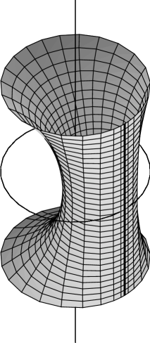
Figure 1. A minimal surface in $\mathbb{H}^{2}\times\mathbb{R}$ foliated by horocycles.

The normal to ${\mathcal{C}}_{0}$ in $\mathbb{H}^{2}\times\mathbb{R}$ is

$$N(u,v)=\left(\begin{array}[]{c}-\frac{v^{2}+1}{2}+\frac{\cos^{2}u}{2}\\ -v\\ \frac{1-v^{2}}{2}+\frac{\cos^{2}u}{2}\\ \sin u\end{array}\right).$$

We compute that the matrix of $\mathrm{S}$ in the frame $(\frac{\partial}{\partial u},\frac{\partial}{\partial v})$ is the following:

$$-\cos u\left(\begin{array}[]{cc}1&0\\ 0&-1\end{array}\right).$$

We also have

$$T=\cos^{2}u\frac{\partial}{\partial u},\quad\nu=\sin u.$$

Minimal surfaces foliated by equidistants.

For $\gamma\in(0,1)$ or $\gamma\in(-1,0)$, we consider the following immersion:

$$x(u,v)=\left(\begin{array}[]{c}\cosh\chi(u)\cosh\gamma v\\ \sinh\chi(u)\\ \cosh\chi(u)\sinh\gamma v\\ u\end{array}\right).$$

with

(15) $$1+\chi^{\prime}(u)^{2}=\gamma^{2}\cosh^{2}\chi(u),\quad\chi^{\prime\prime}(u)=\gamma^{2}\cosh\chi(u)\sinh\chi(u).$$

It is a conformal minimal immersion.

We choose $\chi$ such that $\chi^{\prime}(0)=0$ and $\chi(u)>0$. The function $\chi$ is defined on the interval $(-u_{0},u_{0})$ with

$$u_{0}=\int_{\chi(0)}^{\infty}\frac{\mathrm{d}\chi}{\sqrt{\gamma^{2}\cosh^{2}\chi-1}}=\int_{1}^{\infty}\frac{\mathrm{d}x}{\sqrt{(x^{2}-\gamma^{2})(x^{2}-1)}}.$$

Thus we have

$$u_{0}>\int_{1}^{\infty}\frac{\mathrm{d}x}{x\sqrt{x^{2}-1}}=\frac{\pi}{2}.$$

We have defined a minimal surface ${\mathcal{G}}_{\gamma}$, which we call a generalized catenoid. Its height is greater than $\pi$, tends to $\pi$ when $\gamma\to 0$ and to $+\infty$ when $\gamma\to 1$. The function $\chi$ is decreasing on $(-u_{0},0)$ and increasing on $(0,u_{0})$. The surface is symmetric with respect to the horizontal plane $\mathbb{H}^{2}\times\{0\}$ and it is invariant by a one-parameter family of horizontal hyperbolic isometries. The horizontal curves are equidistants to a geodesic in $\mathbb{H}^{2}$.

The normal to ${\mathcal{G}}_{\gamma}$ in $\mathbb{H}^{2}\times\mathbb{R}$ is

$$N(u,v)=-\frac{1}{\gamma\cosh\chi(u)}\left(\begin{array}[]{c}\sinh\chi(u)\cosh\gamma v\\ \cosh\chi(u)\\ \sinh\chi(u)\sinh\gamma v\\ -\chi^{\prime}(u)\end{array}\right).$$

We compute that the matrix of $\mathrm{S}$ in the frame $(\frac{\partial}{\partial u},\frac{\partial}{\partial v})$ is the following:

$$-\frac{\gamma\sinh\chi(u)}{1+\chi^{\prime}(u)^{2}}\left(\begin{array}[]{cc}1&0\\ 0&-1\end{array}\right).$$

We also have

$$T=\frac{1}{1+\chi^{\prime}(u)^{2}}\frac{\partial}{\partial u},\quad\nu=\frac{\chi^{\prime}(u)}{\gamma\cosh\chi(u)}.$$

Remark 4.18.

When $\gamma=\pm 1$, the formula defines a vertical plane $\mathbb{H}^{1}\times\mathbb{R}$.

Proposition 4.19.

The conjugate surface of the catenoid ${\mathcal{C}}_{\alpha}$ is the helicoid ${\mathcal{H}}_{\beta}$ with $\beta^{2}=1+\alpha^{2}$ and $\alpha$, $\beta$ having the same sign.

Proof.

We set $y_{1}(u)=\alpha\cosh\psi(u)$ and $y_{2}(u)=\beta\cosh\varphi(u)$. A computation shows that both $y_{1}$ and $y_{2}$ are solutions of the following equation:

$$(y^{\prime})^{2}=(y^{2}-\alpha^{2})(y^{2}-\beta^{2}),$$

and hence of the following equation:

$$y^{\prime\prime}=y(2y^{2}-\alpha^{2}-\beta^{2}).$$

We have $\psi^{\prime}(0)=0$ and so by (14) we have $y_{1}(0)^{2}=\beta^{2}$ and thus $y_{1}^{\prime}(0)=0$, and $\varphi(0)=0$ so $y_{2}(0)=\beta$ and thus $y_{2}^{\prime}(0)=0$. Moreover, $y_{1}(0)$ has the sign of $\alpha$, i.e., the sign of $\beta$, so we get $y_{1}(0)=\beta$. By the Cauchy-Lipschitz theorem we conclude that $y_{1}=y_{2}$ (and in particular they have the same domain of definition). From this we deduce using (14) and (13) that $\varphi^{\prime}(u)^{2}=1+\psi^{\prime}(u)^{2}$, and thus ${\mathcal{C}}_{\alpha}$ and ${\mathcal{H}}_{\beta}$ are locally isometric, $\mathrm{S}_{{\mathcal{H}}_{\beta}}=\mathrm{J}\mathrm{S}_{{\mathcal{C}}_{\alpha}}$ and $T_{{\mathcal{H}}_{\beta}}=\mathrm{J}T_{{\mathcal{C}}_{\alpha}}$. Finally we have $\nu_{{\mathcal{C}}_{\alpha}}=\frac{y_{1}^{\prime}}{y_{1}^{2}-\alpha^{2}}$ and $\nu_{{\mathcal{H}}_{\beta}}=\frac{y_{2}^{\prime}}{y_{2}^{2}-\alpha^{2}}$, so we get $\nu_{{\mathcal{H}}_{\beta}}=\nu_{{\mathcal{C}}_{\alpha}}$. ∎

Proposition 4.20.

The conjugate surface of the surface ${\mathcal{C}}_{0}$ is the helicoid ${\mathcal{H}}_{1}$.

Proof.

In the case where $\beta=1$, the function $\varphi$ satisfies $\varphi^{\prime}=\cosh\varphi$, and thus we have $\varphi(u)=\ln(\tan(\frac{u}{2}+\frac{\pi}{4}))$, $\varphi^{\prime}(u)=\frac{1}{\cos u}$ and $\sinh\varphi(u)=\tan u$. Then, using the above calculations, we easily check that ${\mathcal{C}}_{0}$ and ${\mathcal{H}}_{1}$ are locally isometric, and that $\mathrm{S}_{{\mathcal{H}}_{1}}=\mathrm{J}\mathrm{S}_{{\mathcal{C}}_{0}}$, $T_{{\mathcal{H}}_{1}}=\mathrm{J}T_{{\mathcal{C}}_{0}}$, $\nu_{{\mathcal{H}}_{1}}=\nu_{{\mathcal{C}}_{0}}$. ∎

Remark 4.21.

The conjugate surface of the surface ${\mathcal{C}}_{0}$ with the opposite orientation is the helicoid ${\mathcal{H}}_{-1}$.

Proposition 4.22.

The conjugate surface of the generalized catenoid ${\mathcal{G}}_{\gamma}$ is the helicoid ${\mathcal{H}}_{\beta}$ with $\beta^{2}+\gamma^{2}=1$ and $\beta$, $\gamma$ having the same sign.

Proof.

We set $y_{1}(u)=\gamma\sinh\chi(u)$ and $y_{2}(u)=\beta\cosh\varphi(u)$. A computation shows that both $y_{1}$ and $y_{2}$ are solutions of the following equation:

$$(y^{\prime})^{2}=(y^{2}+\gamma^{2})(y^{2}-\beta^{2}),$$

and hence of the following equation:

$$y^{\prime\prime}=y(2y^{2}+\gamma^{2}-\beta^{2}).$$

We have $\chi^{\prime}(0)=0$ and so by (15) we have $y_{1}(0)^{2}=\beta^{2}$ and thus $y_{1}^{\prime}(0)=0$, and $\varphi(0)=0$ so $y_{2}(0)=\beta$ and thus $y_{2}^{\prime}(0)=0$. Moreover, $y_{1}(0)$ has the sign of $\gamma$, i.e., the sign of $\beta$, so we get $y_{1}(0)=\beta$. By the Cauchy-Lipschitz theorem we conclude that $y_{1}=y_{2}$ (and in particular they have the same domain of definition). From this we deduce using (15) and (13) that $\varphi^{\prime}(u)^{2}=1+\chi^{\prime}(u)^{2}$, and thus ${\mathcal{G}}_{\gamma}$ and ${\mathcal{H}}_{\beta}$ are locally isometric, $\mathrm{S}_{{\mathcal{H}}_{\beta}}=\mathrm{J}\mathrm{S}_{{\mathcal{G}}_{\gamma}}$ and $T_{{\mathcal{H}}_{\beta}}=\mathrm{J}T_{{\mathcal{G}}_{\gamma}}$. Finally we have $\nu_{{\mathcal{G}}_{\gamma}}=\frac{y_{1}^{\prime}}{y_{1}^{2}+\gamma^{2}}$ and $\nu_{{\mathcal{H}}_{\beta}}=\frac{y_{2}^{\prime}}{y_{2}^{2}+\gamma^{2}}$, so we get $\nu_{{\mathcal{H}}_{\beta}}=\nu_{{\mathcal{G}}_{\gamma}}$. ∎

Remark 4.23.

This study shows that there are three types of helicoid conjugates according to the parameter of the screw-motion associated to the helicoid: the first type ones are the catenoids, which are rotational surfaces, the second type one is ${\mathcal{C}}_{0}$, which is invariant by a one-parameter family of horizontal parabolic isometries and which corresponds to a critical value of the parameter, the third type ones are the generalized catenoids, which are invariant a one-parameter family of horizontal hyperbolic isometries.

This phenomenon is very similar to what happens for the conjugate cousins in $\mathbb{H}^{3}$ of the helicoids in $\mathbb{R}^{3}$. There exists an isometric correspondance between minimal surfaces in $\mathbb{R}^{3}$ and constant mean curvature one surfaces in $\mathbb{H}^{3}$ called the cousin relation (see [Bry87] and [UY93]). Starting from a helicoid in $\mathbb{R}^{3}$, we consider its conjugate surface, which is a catenoid in $\mathbb{R}^{3}$, and then the cousin surface in $\mathbb{H}^{3}$, which is a catenoid cousin. Catenoid cousins are of three types according to the parameter of the minimal helicoid: some are rotational surfaces, one is invariant by a one-parameter family of parabolic isometries (and corresponds to a critical value of the parameter), some are invariant by a one-parameter family of hyperbolic isometries. These surfaces are described in details in [SET01] and [Ros02a].

Remark 4.24.

All the above surfaces belong to the Hauswirth family: with the notations of [Hau03], helicoids correspond to $d=0$, $c>0$, $c\neq 1$; catenoids correspond to $c=0$, $d>1$; the surface ${\mathcal{C}}_{0}$ corresponds to $c=0$, $d=1$; the surfaces ${\mathcal{G}}_{\gamma}$ correspond to $c=0$, $d\in(0,1)$.

Remark 4.25.

The vertical plane $\mathbb{H}^{1}\times\mathbb{R}$ is globally invariant by conjugation, but the vertical lines and the horizontal geodesics of $\mathbb{H}^{2}$ are exchanged. The horizontal plane $\mathbb{H}^{2}\times\{0\}$ is pointwise invariant by conjugation (since it satisfies $\mathrm{S}=0$ and $T=0$). This is similar to what happens in $\mathbb{S}^{2}\times\mathbb{R}$.

References

- [AR03] U. Abresch and H. Rosenberg. The Hopf differential for constant mean curvature surfaces in and . Preprint, 2003.
- [Bry87] R. Bryant. Surfaces of mean curvature one in hyperbolic space. Astérisque, 154–155:321–347, 1987.
- [Car92] M. do Carmo. Riemannian Geometry. Birkhäuser, 1992.
- [Hau03] L. Hauswirth. Generalized Riemann examples in three-dimensional manifolds. Preprint, 2003.
- [HSET04] L. Hauswirth, R. Sá Earp, and É. Toubiana. Minimal surfaces in . Work in progress, 2004.
- [Kar01] H. Karcher. Introduction to conjugate Plateau constructions. Preprint, 2001.
- [MR03] W. Meeks and H. Rosenberg. The theory of minimal surfaces in . Preprint, 2003.
- [NR02] B. Nelli and H. Rosenberg. Minimal surfaces in . Bull. Braz. Math. Soc., New Series, 33(2):263–292, 2002.
- [PR99] R. Pedrosa and M. Ritoré. Isoperimetric domains in the Riemannian product of a circle with a simply connected space form and applications to free boundary value problems. Indiana Univ. Math. J., 48:1357–1394, 1999.
- [Ros02a] H. Rosenberg. Bryant surfaces. In The Global Theory of Minimal Surfaces in Flat Spaces, Martina Franca, Italy 1999, Lecture Notes in Mathematics 1775. Springer, 2002.
- [Ros02b] H. Rosenberg. Minimal surfaces in . Illinois J. Math., 46(4):1177–1195, 2002.
- [Ros03] H. Rosenberg. Some recent developments in the theory of minimal surfaces in -manifolds. In 24o Colóquio Brasileiro de Matemática, Instituto de Matemática Pura e Aplicada, Rio de Janeiro. Publicações Matemáticas do IMPA, 2003.
- [SET01] R. Sá Earp and É. Toubiana. On the geometry of constant mean curvature one surfaces in hyperbolic space. Illinois J. Math., 45(2):371–401, 2001.
- [SET04] R. Sá Earp and É. Toubiana. Screw motion surfaces in and . Preprint, 2004.
- [SY97] R. Schoen and S. T. Yau. Lectures on Harmonic Maps. Conference Proceedings and Lecture Notes in Geometry and Topology, II. International Press, Cambridge, MA, 1997.
- [Ten71] K. Tenenblat. On isometric immersions of Riemannian manifolds. Bol. Soc. Brasil. Mat., 2(2):23–36, 1971.
- [UY93] M. Umehara and K. Yamada. Complete surfaces of constant mean curvature in the hyperbolic -space. Ann. of Math. (2), 137:611–638, 1993.