Diffusion local time storage

In this paper we study a storage process or a liquid queue in which the input process is the local time of a positively recurrent stationary diffusion in stationary state and the potential output takes place with a constant deterministic rate. For this storage process we find its stationary distribution and compute the joint distribution of the starting and ending times of the busy and idle periods. This work completes and extends to a more general setting the results in Mannersalo, Norros, and Salminen [9].

MSC: 60G10; 60J55; 60J60; 60K25

Keywords: Brownian motion with drift; Busy and idle periods; Diffusion processes; Palm probability; Spectrally positive Lévy processes

1 Introduction

Let $A=\{A_{t}:t\in\mathbb{R}\}$ and $B=\{B_{t}:t\in\mathbb{R}\}$ be increasing stochastic processes. We view $A$ as the input process to a storage or a buffer and $B$ as the potential output. One of the standard ways to define a storage process associated to $A$ and $B$ is via Reich’s formula (see Reich [11])

$$S_{t}:=\sup_{-\infty<s\leq t}\{A_{t}-A_{s}-(B_{t}-B_{s})\},\quad t\in\mathbb{R}.$$

We refer also to Prabhu [10] p. 114 for an approach in which the storage process is defined as a solution of a stochastic integral equation and the input process $A$ is a subordinator without drift and $B_{t}=t$. In Harrison [7] p. 14 the case in which $A$ is a Brownian motion and $B_{t}=\mu t$ is studied via Skorohod’s reflection equation. Brownian motion, although not increasing, is much analyzed input process and its appearence in these models can be motivated in different ways, see, e.g., Harrison [7] p. 30, Roberts, Mocci and Virtamo [12] p. 377, and Salminen and Norros [salminennorros01]. A new kind of a model is introduced in Mannersalo, Norros, and Salminen [9], in which the local time at 0 of a reflected Brownian motion with negative drift serves as the input process. Recall that this local time process is increasing and continuous but the points of its increase form a singular set.

In this paper, we consider a model of a storage or a fluid queue, where the input is the local time $L$ at zero of an arbitrary one-dimensional positively recurrent stationary diffusion and the potential output $B_{t}=\mu t$, $\mu>0$; thus extending the approach in [9]. Recall that any subordinator can be viewed as the inverse local time of a strong Markov process. Hence, in a sense, the local time storage models are companions of the subordinator storage models and as such interesting objects of research.

It is shown in [9] that the storage model studied therein can be obtained via a limiting procedure from some on/off processes. Especially, a priority discrete queueing system is constructed which, when in heavy traffic, leads to a storage process with local time input. The proof of weak convergence in [9] is based on the continuous mapping theorem and the interpretation of the Brownian local time as a supremum process. However, this approach is not applicable in our general case, and we do not discuss here the weak converegence aspects of our model.

Further, in [9] the joint distribution of the starting time $g_{i}$ and the ending time $d_{i}$ of an idle period and the marginal distributions of the starting time $g_{b}$ and the ending time $d_{b}$ of a busy period are obtained. The joint distribution of $g_{b}$ and $d_{b}$ is not, however, given in [9]. The aim of this paper is to fill this gap and to generalize the results to an arbitrary diffusion local time storage.

We give explicit expressions for the joint Laplace transforms of the starting and the ending times of the busy and idle periods. Surprisingly, the answers have a short simple form, expressed in terms of the Lévy-Khinchin exponent of the inverse of the local time process $L.$ By considering a marked point process obtained from the storage process $S$ we make the simple but crucial observation needed for finding the joint distributions. This observation, formulated here only for the busy period, is that the random variable $(-g_{b},d_{b})$ is identical in law with $(UV,(1-U)V)$, where $U$ has the uniform distribution on $(0,1)$ and $V$ is a positive random variable independent of $U$ having the distribution of the length of the busy period. In particular, which is important here, we show that the joint Laplace transform of such variables can be easily expressed in terms of the marginal Laplace transforms.

We remark also that in [9] the marginal distribution of $-g_{b}$ is computed by making use of Bertoin’s path decomposition theorem (see Bertoin [3]). However, in this paper we focus instead on $d_{b}$. It is seen that the formula for the first time when a spectrally positive Lévy process jumps over a level, see (3.9), can be applied to find the Laplace transform of $d_{b}.$

The paper is organized as follows. In the next section we give some definitions and construct the storage process with a diffusion local time input. It is important to verify here that our local time process has stationary increments. It is also proved that the stationary distribution of this storage process is always exponential with an atom at zero - only the value of the parameter and the size of the atom vary when the underlying diffusion is changed. In Section 3, the Laplace transform of the ending time $d_{b}$ of a busy period observed at time zero is computed. In Section 4, we find the Laplace transform of the starting time $g_{i}$ of an idle period observed at time zero. Theorem 5.1 in Section 5 can be viewed as the main result of the paper, where the joint distributions of $(-g_{b},d_{b})$ and $(-g_{i},d_{i})$ are given via their Laplace transforms. Finally, in Section 6, we discuss the case treated in [9]. In particular, we invert the Laplace transforms to obtain the joint densities of $(-g_{i},d_{i})$ and $(-g_{b},d_{b})$.

2 Definitions and preliminaries

Let $X=\{X_{t}:t\geq 0\}$ be a one-dimensional time-homogeneous, regular, conservative diffusion living in an interval $I\subseteq\mathbb{R}$. We assume, without loss of generality, that $0\in I$. The probability measure and the expectation associated with $X$ started at $x$, are denoted by $\mathbf{P}_{x}$ and $\mathbf{E}_{x}$, respectively. Recall that $X$ has a symmetric transition density with respect to its speed measure $m$:

$$\mathbf{P}_{x}(X_{t}\in dy)=p(t;x,y)m(dy)=p(t;y,x)m(dy).$$

We introduce also the Green function

$$G_{\alpha}(x,y)=\int_{0}^{\infty}e^{-\alpha t}p(t;x,y)dt,\quad x,y\in I,\>\alpha\geq 0.$$

Further, it is assumed that $X$ is positively recurrent, that is, the speed measure is finite in $I$. Denote $M:=m\{I\}<+\infty$. For more details on linear diffusions we refer to Itô and McKean [8] and Borodin and Salminen [5].

Let $X^{(1)}$ and $X^{(2)}$ be two copies of $X$. We take $X_{0}^{(1)}=X_{0}^{(2)}$ with the common distribution

$$\mathbf{P}(X_{0}^{(1)}\in dx)=\mathbf{P}(X_{0}^{(2)}\in dx)=\frac{m(dx)}{M}=:\widehat{m}(dx)$$

but otherwise we let $X^{(1)}$ and $X^{(2)}$ be independent. We remark that $\widehat{m}$ is the stationary probability distribution of $X.$ Define $Z=\{Z_{t}:t\in\mathbb{R}\}$ as

$$Z_{t}:=\left\{\begin{array}[]{cc}X_{-t}^{(1)}&\mbox{if $t\leq 0$},\\ X_{t}^{(2)}&\mbox{if $t\geq 0$}.\end{array}\right.$$

The process $Z$ thus defined is a stationary process in stationary state.

Let $\{L_{t}^{(1)}:t\geq 0\}$ and $\{L_{t}^{(2)}:t\geq 0\}$ be the local times at zero of the processes $X^{(1)}$ and $X^{(2)}$, respectively. We choose the normalization of $L^{(i)}$, $i=1,2$, with respect to the speed measure, that is,

$$L_{t}^{(i)}:=\lim_{\varepsilon\searrow 0}\frac{1}{m\{(-\varepsilon,\varepsilon)\}}\int_{0}^{t}\mathbf{1}_{(-\varepsilon,\varepsilon)}(X_{s}^{(i)})\,ds,\quad i=1,2.$$ (2.1)

Using $L^{(1)}$ and $L^{(2)}$, we define the local time process $L=\{L_{t}:t\in\mathbb{R}\}$ via

$$L_{t}:=\left\{\begin{array}[]{cc}-L_{-t}^{(1)}&\mbox{if $t\leq 0$},\\ L_{t}^{(2)}&\mbox{if $t\geq 0$}.\end{array}\right.$$

The process $L$ is an increasing continuous process passing through zero at time zero. Next we give an important property of $L$, which allows us to construct a stationary storage process.

Proposition 2.1.

The process $L$ has stationary increments, i.e., for all $t>~{}s$,

$$L_{t}-L_{s}\stackrel{{\scriptstyle d}}{{=}}L_{t-s}.$$

Moreover,

$$\mathbf{E}(L_{t})=t/M.$$ (2.2)

Proof: Consider first the case $t>s>0$. Then, using that $Z$ is a stationary process in stationary state, we have

$$\mathbf{P}(L_{t}-L_{s}\in dl) = \int_{I}\widehat{m}(dx)\mathbf{P}(L_{t}-L_{s}\in dl\,|\,Z_{s}=x)$$

$$= \int_{I}\widehat{m}(dx)\mathbf{P}_{x}(L_{t-s}\in dl)$$

$$= \mathbf{P}(L_{t-s}\in dl).$$

The case $s<t<0$ is treated similarly. Assume next that $s<0<t$. Then by the conditional independence of $X^{(1)}$ and $X^{(2)}$ given $Z_{0}$ we can write

$$\mathbf{E}(e^{-\alpha(L_{t}-L_{s})}) = \mathbf{E}(e^{-\alpha(L_{t}^{(1)}+L_{-s}^{(2)})})$$

$$= \int_{I}\widehat{m}(dx)\mathbf{E}_{x}(e^{-\alpha L_{t}^{(1)}})\mathbf{E}_{x}(e^{-\alpha L_{-s}^{(2)}}).$$

On the other hand, consider

$$\mathbf{E}(e^{-\alpha L_{t-s}}) = \mathbf{E}(e^{\alpha(L_{t-s}-L_{-s}+L_{-s})})$$

$$= \int_{I}\widehat{m}(dx)\int_{I}\mathbf{E}_{x}(e^{-\alpha L_{-s}}\,;\,Z_{-s}\in dy)\mathbf{E}(e^{\alpha(L_{t-s}-L_{-s})}\,|\,Z_{-s}=y).$$

Let now $\tau$ be an exponentially distributed random variable with parameter $\alpha$ independent of $X^{(2)}$, and define the killed process

$$X_{t}^{\bullet}:=\left\{\begin{array}[]{cc}X_{t}^{(2)}&\mbox{if $L_{t}^{(2)}<\tau$},\\ \triangle&\mbox{if $L_{t}^{(2)}\geq\tau$},\end{array}\right.$$

where $\triangle$ is a cemetery point. Then (see Borodin and Salminen [5] p. 28 or Itô and McKean [8] p. 179-183) $X_{t}^{\bullet}$ is a diffusion having the same speed measure as $X^{(2)}$. Let $p^{\bullet}(t;x,y)$ be its (symmetric) transition density with respect to $m$. We clearly have

$$\mathbf{P}_{x}(X_{t}^{\bullet}\in dy) = \mathbf{P}_{x}(X_{t}^{(2)}\in dy,L_{t}^{(2)}<\tau)$$

$$= \mathbf{E}_{x}(e^{-\alpha L_{t}^{(2)}}\,;\,X_{t}^{(2)}\in dy)$$

$$= p^{\bullet}(t;x,y)\,m(dy).$$

From the symmetry of $p^{\bullet}(t;x,y)$ it follows that

$$\int_{I}m(dx)\mathbf{E}_{x}(e^{-\alpha L_{-s}}\,;\,Z_{-s}\in dy)=m(dy)\mathbf{E}_{y}(e^{-\alpha L_{-s}}),$$

and, therefore,

$$\mathbf{E}(e^{-\alpha L_{t-s}}) = \int_{I}\widehat{m}(dy)\mathbf{E}_{y}(e^{-\alpha L_{-s}})\mathbf{E}(e^{-\alpha(L_{t-s}-L_{-s})}\,|\,Z_{-s}=y)$$

$$= \int_{I}\widehat{m}(dy)\mathbf{E}_{y}(e^{-\alpha L_{-s}})\mathbf{E}_{y}(e^{-\alpha L_{t}})$$

$$= \mathbf{E}(e^{-\alpha(L_{t}-L_{s})}),$$

as claimed. Finally, to show $(\ref{mean})$ recall the formula (see Itô and McKean [8] p. 175 or Borodin and Salminen [5] p. 21)

$$\mathbf{E}_{x}(L_{t})=\int_{0}^{t}p(s;x,0)\,ds,\quad t>0.$$

Consequently,

$$\mathbf{E}(L_{t}) = \int_{I}\widehat{m}(dx)\int_{0}^{t}ds\,p(s;x,0)$$

$$= \int_{0}^{t}ds\int_{I}\widehat{m}(dx)\,p(s;x,0)$$

$$= \int_{0}^{t}ds\int_{I}\widehat{m}(dx)\,p(s;0,x)$$

$$= t/M,$$

because

$$\int_{I}m(dx)\,p(s;0,x)=1.$$

∎

Definition 2.2.

The process $S=\{S_{t}:t\in\mathbb{R}\}$ defined as

$$S_{t}:=\sup_{-\infty<s\leq t}\{L_{t}-L_{s}-\mu(t-s)\},\quad t\in\mathbb{R}$$

is called a storage process with local time input, constant service rate $\mu$, and unbounded buffer associated with the process $Z$.

Because the process $L$ has stationary increments it follows from Definition 2.2 that $S$ is a stationary process (in stationary state). Our next task is to find its stationary distribution, that is, the distribution of $S_{0}$. Notice that $S_{0}$ is determined by the process $X^{(1)}$. With a slight and short abuse of our notations, let $\{L^{(1)}_{t}:t\geq 0\}$ be the local time of $X^{(1)}$ started at zero normalized as in $(\ref{eqloc})$. Then the process $A^{(1)}$ given by

$$A^{(1)}_{t}:=\inf\{s:L^{(1)}_{s}>t\},\quad t\geq 0$$

is a subordinator (a right-continuous increasing process on $\mathbb{R}_{+}$ with independent and stationary increments). When normalizing as in (2.1) we have (see Itô and McKean [8], p. 214) that

$$\mathbf{E}_{0}(\exp\{-\alpha A^{(1)}_{t}\})=\exp\left\{-\frac{t}{G_{\alpha}(0,0)}\right\},$$ (2.3)

and, therefore,

$$\mathbf{E}_{0}\left(\exp\{-\alpha(A^{(1)}_{t}-t/\mu)\}\right)=\exp\left\{-t\left(\frac{1}{G_{\alpha}(0,0)}-\frac{\alpha}{\mu}\right)\right\}=\exp\{t\psi(\alpha)\},$$

where the function

$$\psi(\alpha)=\frac{\alpha}{\mu}-\frac{1}{G_{\alpha}(0,0)}$$ (2.4)

is called the Lévy-Khintchin exponent of the spectrally positive Lévy process $\{A^{(1)}_{t}-t/\mu\,:\,t\geq 0\}$.

Proposition 2.3.

Assume that $\mu>1/M$, in other words $\mu>\mathbf{E}(L_{1})$. Then the equation

$$\psi(\alpha)=0$$ (2.5)

has a unique positive solution $\alpha^{*}$. Moreover,
1) $\displaystyle{\mathbf{P}(S_{0}>t|Z_{0}=x)=\mathbf{E}\left(e^{-\alpha^{*}H_{0}}|Z_{0}=x\right)e^{-\frac{\alpha^{*}}{\mu}t},\quad t\geq 0,\;x\in I}$,
where $H_{0}:=\inf\{t\geq 0:\,Z_{t}=0\}$;
2) the process $S$ is stationary with the stationary distribution given by

$$\mathbf{P}(S_{t}>y)=\frac{1}{M\mu}e^{-\frac{\alpha^{*}}{\mu}y},\quad y\geq 0,$$

and $\mathbf{P}(S_{t}=0)=1-\frac{1}{M\mu}$.

Proof: The stationarity follows from Proposition 2.1. The other claims follow from the fact that the spectrally positive Lévy process $\{A^{(1)}_{t}-t/\mu\,:\,t\geq 0\}$ drifts to $+\infty$ and its infimum is exponentially distributed in $\mathbb{R}_{-}$ with parameter $\alpha^{*}.$ For further details, see [13]. ∎

Remark 2.4.

1) The Laplace transform of $H_{0}$ appearing above can be expressed as

$$\mathbf{E}_{x}\left(e^{-\alpha H_{0}}\right)=\frac{G_{\alpha}(x,0)}{G_{\alpha}(0,0)},$$ (2.6)

cf. Borodin and Salminen [5], p. 18.
2) Recall (cf. Bingham [4] p. 720) that for $\alpha\geq\alpha^{*}$, the function $\psi(\alpha)$ is positive and increasing and, hence, has an inverse which we denote by $\alpha\mapsto\eta(\alpha)$.
3) From Proposition 2.3 it is clear that $S_{0}$, conditionally on $S_{0}>0$, is exponentially distributed with parameter $\alpha^{*}/\mu$.

We assume throughout the paper that $\mu>1/M$. Next we define the subject of our main interest in this work, the on-going busy and idle periods of $S$.

Definition 2.5.

If $S_{0}=0$ then the random variables

$$g_{i}=\sup\{t<0:S_{t}>0\}\quad\mbox{\rm and}\quad d_{i}=\inf\{t>0:S_{t}>0\}$$

are called the starting time and the ending time, respectively, of the on-going idle period at time zero. If $S_{0}>0$ then the random variables

$$g_{b}=\sup\{t<0:S_{t}=0\}\quad\mbox{\rm and}\quad d_{b}=\inf\{t>0:S_{t}=0\}$$

are called the starting time and the ending time, respectively, of the on-going busy period at time zero.

3 Busy periods

In this section we compute the Laplace transform of the ending time of the on-going busy period. It is shown in Mannersalo, Norros, and Salminen [9] using a point process view on the busy and idle periods that $-g_{b}$ and $d_{b}$ have the same law. In the present paper (in Section 5) we develop this approach in order to find the joint distribution of $-g_{b}$ and $d_{b}$.

From Proposition 2.3 it is seen that the probability that there is a busy period at time zero is $1/(M\mu)$.

Theorem 3.1.

Let $\eta$ be the inverse of $\psi$ (cf. Remark $\ref{rema1}.2$). Then

$$\mathbf{E}(e^{-\alpha d_{b}}\,|\,S_{0}>0)=\frac{\alpha^{*}}{\eta(\alpha/\mu)}.$$ (3.1)

The rest of this section is devoted to the proof of Theorem 3.1. Assuming that there is a busy period at 0 we have (cf. [9])

$$S_{t}=L_{t}-\mu t+S_{0},\quad g_{b}\leq t\leq d_{b}.$$

Let $H_{0}^{(2)}$ be the first hitting time of zero for the process $X^{(2)}$. Because

$$S_{0}=\sup_{s\leq 0}\{\mu s-L_{s}\}=\sup_{s\leq 0}\{\mu s+L_{-s}^{(1)}\}$$

it follows that $S_{0}$ and $H_{0}^{(2)}$ are conditionally independent, given $Z_{0}$ . The local time $L_{t}=0$ when $0\leq t\leq H_{0}^{(2)}$. Hence,

$$S_{t}=S_{0}-\mu t,\quad 0\leq t\leq\min\{H_{0}^{(2)},S_{0}/\mu\}.$$

To proceed consider, therefore, two cases:

1)

$S_{0}/\mu<H_{0}^{(2)}$,

2)

$S_{0}/\mu>H_{0}^{(2)}$ (see Figure 1).

In the case 1) we obviously have

$$\{S_{0}/\mu<H_{0}^{(2)}\,,\,S_{0}>0\}=\{d_{b}=S_{0}/\mu\,,\,S_{0}>0\}.$$ (3.2)

To analyze the case 2), we study in detail some relationships between $S_{0}$ and $H_{0}^{(2)}$. Firstly, introduce

$$J(\alpha,\beta):=\int_{I}m(dx)\mathbf{E}_{x}(e^{-\alpha H_{0}})\mathbf{E}_{x}(e^{-\beta H_{0}}),\quad\alpha\geq 0,\>\beta\geq 0.$$ (3.3)

Proposition 3.2.

$$\mathbf{E}\left(e^{-\alpha(S_{0}/\mu-H_{0}^{(2)})-\beta H_{0}^{(2)}}\,,\,S_{0}/\mu>H_{0}^{(2)}\right)=\frac{\alpha^{*}}{\alpha+\alpha^{*}}\frac{1}{M}J(\alpha^{*},\alpha^{*}+\beta).$$ (3.4)

Proof: Using Proposition 2.3 and the conditional independence of $S_{0}$ and $H_{0}^{(2)}$ given $Z_{0}$, we compute the joint Laplace transform as follows:

$$\mathbf{E}\left(e^{-\alpha(S_{0}/\mu-H_{0}^{(2)})-\beta H_{0}^{(2)}}\,,\,S_{0}/\mu>H_{0}^{(2)}\right)$$

$$\hskip 19.91684pt=\int_{I}\widehat{m}(dx)\mathbf{E}_{x}\left(e^{-\alpha(S_{0}/\mu-H_{0}^{(2)})-\beta H_{0}^{(2)}}\,,\,S_{0}/\mu>H_{0}^{(2)}\right)$$

$$\hskip 19.91684pt=\int_{I}\widehat{m}(dx)\int_{0}^{\infty}\mathbf{E}_{x}\left(e^{-\alpha(S_{0}/\mu-t)}e^{-\beta t}\,,\,S_{0}/\mu>t\right)\mathbf{P}_{x}(H_{0}^{(2)}\in dt)$$

$$\hskip 19.91684pt=\int_{I}\widehat{m}(dx)\int_{0}^{\infty}e^{(\alpha-\beta)t}\mathbf{P}_{x}(H_{0}^{(2)}\in dt)\int_{t}^{\infty}e^{-\alpha u}\mathbf{P}_{x}(S_{0}/\mu\in du)$$

$$\hskip 19.91684pt=\int_{I}\widehat{m}(dx)\int_{0}^{\infty}e^{(\alpha-\beta)t}\mathbf{P}_{x}(H_{0}^{(2)}\in dt)\int_{t}^{\infty}e^{-\alpha u}\alpha^{*}e^{-\alpha^{*}u}\mathbf{E}_{x}(e^{-\alpha^{*}H_{0}})du$$

$$\hskip 19.91684pt=\frac{\alpha^{*}}{\alpha+\alpha^{*}}\frac{1}{M}\int_{I}m(dx)\int_{0}^{\infty}e^{(\alpha-\beta)t}\mathbf{P}_{x}(H_{0}^{(2)}\in dt)\mathbf{E}_{x}(e^{-\alpha^{*}H_{0}})e^{-(\alpha+\alpha^{*})t}$$

$$\hskip 19.91684pt=\frac{\alpha^{*}}{\alpha+\alpha^{*}}\frac{1}{M}\int_{I}m(dx)\mathbf{E}_{x}(e^{-\alpha^{*}H_{0}})\mathbf{E}_{x}(e^{-(\alpha^{*}+\beta)H_{0}}),$$

as claimed. ∎

An immediate consequence of Proposition 3.2 is the following

Corollary 3.3.

1) The random variables $S_{0}/\mu-H_{0}^{(2)}$ and $H_{0}^{(2)}$ are conditionally independent, given that $S_{0}/\mu>H_{0}^{(2)}$.
2) The conditional distribution of $S_{0}/\mu-H_{0}^{(2)}$, given that $S_{0}/\mu>H_{0}^{(2)}$, is exponential with parameter $\alpha^{*}$.
3) $\displaystyle{\mathbf{E}\left(e^{-\alpha H_{0}^{(2)}}\,,\,S_{0}/\mu>H_{0}^{(2)}\right)=\frac{J(\alpha^{*},\alpha^{*}+\alpha)}{M}}.$
4) $\displaystyle{\mathbf{E}\left(e^{-\alpha S_{0}/\mu}\,,\,S_{0}/\mu>H_{0}^{(2)}\right)=\frac{\alpha^{*}}{\alpha+\alpha^{*}}\frac{J(\alpha^{*},\alpha^{*}+\alpha)}{M}}.$

Proposition 3.4.

The functions $J(\alpha^{*},\alpha^{*}+\alpha)$ and $\psi(\alpha)$ defined in $(\ref{j})$ and $(\ref{levy1})$, respectively, satisfy the relationship:

$$J(\alpha^{*},\alpha^{*}+\alpha)=\frac{1}{\mu}-\frac{\psi(\alpha+\alpha^{*})}{\alpha}.$$ (3.5)

Proof: Using formula $(\ref{green})$ and the Chapman-Kolmogorov equation, we compute for any positive $\alpha_{1}\neq\alpha_{2}$,

$$\int_{I}m(dx)\,\mathbf{E}_{x}(e^{-\alpha_{1}H_{0}})\mathbf{E}_{x}(e^{-\alpha_{2}H_{0}})$$

$$\hskip 5.69046pt=\int_{I}m(dx)\,G_{\alpha_{1}}(x,0)G_{\alpha_{2}}(x,0)\,/(G_{\alpha_{1}}(0,0)G_{\alpha_{2}}(0,0))$$

$$\hskip 5.69046pt=\int_{I}m(dx)\int_{0}^{\infty}dt\,e^{-\alpha_{1}t}p(t;x,0)\int_{0}^{\infty}ds\,e^{-\alpha_{2}s}p(s;x,0)/(G_{\alpha_{1}}(0,0)G_{\alpha_{2}}(0,0))$$

$$\hskip 5.69046pt=\int_{0}^{\infty}dt\int_{0}^{\infty}ds\,e^{-\alpha_{1}t-\alpha_{2}s}\int_{I}m(dx)p(t;x,0)p(s;x,0)/(G_{\alpha_{1}}(0,0)G_{\alpha_{2}}(0,0))$$

$$\hskip 5.69046pt=\int_{0}^{\infty}dt\int_{0}^{\infty}ds\,e^{-\alpha_{1}t-\alpha_{2}s}p(t+s,0,0)\,/(G_{\alpha_{1}}(0,0)G_{\alpha_{2}}(0,0))$$

$$\hskip 5.69046pt=\int_{0}^{\infty}du\,\left(\int_{0}^{u}e^{(\alpha_{1}-\alpha_{2})s}ds\right)e^{-\alpha_{1}u}p(u;0,0)\,/(G_{\alpha_{1}}(0,0)G_{\alpha_{2}}(0,0))$$

$$\hskip 5.69046pt=\frac{1}{\alpha_{1}-\alpha_{2}}\int_{0}^{\infty}(e^{-\alpha_{2}u}-e^{-\alpha_{1}u})p(u;0,0)du\,/(G_{\alpha_{1}}(0,0)G_{\alpha_{2}}(0,0))$$

$$\hskip 5.69046pt=\frac{1}{\alpha_{1}-\alpha_{2}}\left(\frac{1}{G_{\alpha_{1}}(0,0)}-\frac{1}{G_{\alpha_{2}}(0,0)}\right).$$

Since

$$\frac{1}{G_{\alpha}(0,0)}=\frac{\alpha}{\mu}-\psi(\alpha),$$

we have

$$J(\alpha_{1},\alpha_{2})=\frac{1}{\mu}-\frac{\psi(\alpha_{1})-\psi(\alpha_{2})}{\alpha_{1}-\alpha_{2}}.$$ (3.6)

Substituting $\alpha^{*}$ for $\alpha_{1}$ and $\alpha+\alpha^{*}$ for $\alpha_{2}$ in $(\ref{ipsi})$ and using that $\psi(\alpha^{*})=0$ give $(\ref{I})$. ∎

To proceed with the proof of Theorem 3.1 write

$$\mathbf{E}(e^{-\alpha d_{b}}\,|\,S_{0}>0) = \mathbf{E}(e^{-\alpha d_{b}}\,,\,S_{0}/\mu<H_{0}^{(2)}\,|\,S_{0}>0)$$ (3.7)

$$\hskip 5.69046pt+\,\mathbf{E}(e^{-\alpha d_{b}}\,,\,S_{0}/\mu>H_{0}^{(2)}\,|\,S_{0}>0).$$

For the first term we obtain by $(\ref{dbs})$, Corollary $\ref{cor1}.4$, and Proposition 2.3

$$\mathbf{E}(e^{-\alpha d_{b}}\,,\,S_{0}/\mu<H_{0}^{(2)}\,|\,S_{0}>0)$$

$$\hskip 19.91684pt=\mathbf{E}(e^{-\alpha S_{0}/\mu}\,,\,S_{0}/\mu<H_{0}^{(2)}\,|\,S_{0}>0)$$

$$\hskip 19.91684pt=\mathbf{E}(e^{-\alpha S_{0}/\mu}\,|\,S_{0}>0)-\mathbf{E}(e^{-\alpha S_{0}/\mu}\,,\,S_{0}/\mu>H_{0}^{(2)}\,|\,S_{0}>0)$$

$$\hskip 19.91684pt=\mathbf{E}(e^{-\alpha S_{0}/\mu}\,|\,S_{0}>0)-\frac{\mathbf{E}(e^{-\alpha S_{0}/\mu}\,,\,S_{0}/\mu>H_{0}^{(2)})}{\mathbf{P}(S_{0}>0)}$$

$$\hskip 19.91684pt=\frac{\alpha^{*}}{\alpha+\alpha^{*}}\big{(}1-\mu J(\alpha^{*},\alpha^{*}+\alpha)\big{)}.$$ (3.8)

To compute the second term in $(\ref{dbsumma})$ consider the process

$$\widetilde{X}=\{X_{H_{0}^{(2)}+t}:t\geq 0\}.$$

By the strong Markov property $\widetilde{X}$ has the same law as $X^{(2)}$ started at zero. Let $\widetilde{L}=\{\widetilde{L_{t}}:t\geq 0\}$ be the local time at zero of $\widetilde{X}$, that is, the local time of $X^{(2)}$ started at zero. Let $\widetilde{A}$ be the right continuous inverse of $\widetilde{L}$ and introduce

$$T^{+}_{t}:=\inf\{s:\widetilde{A}_{s}-s/\mu>t\},\quad t>0.$$

Observe next that in the case $S_{0}/\mu>H_{0}^{(2)}$ (see Figure 1) we have

$$d_{b}=\frac{1}{\mu}\,T^{+}_{S_{0}/\mu-H_{0}^{(2)}}+\frac{S_{0}}{\mu}.$$

Using this representation and conditional independence stated in Corollary $\ref{cor1}.1$, it is seen that

$$\mathbf{E}\left(e^{-\alpha d_{b}}\,,\,S_{0}/\mu>H_{0}^{(2)}\,\big{|}\,S_{0}>0\right)$$

$$\hskip 19.91684pt=\mathbf{E}\left(e^{-\alpha d_{b}}\,\big{|}\,S_{0}/\mu>H_{0}^{(2)}\right)\mathbf{P}\left(S_{0}/\mu>H_{0}^{(2)}\,\big{|}\,S_{0}>0\right)$$

$$\hskip 19.91684pt=\mathbf{E}\left(\exp\left\{-\alpha\left(\frac{1}{\mu}\,T^{+}_{S_{0}/\mu-H_{0}^{(2)}}+\frac{S_{0}}{\mu}\right)\right\}\,\Big{|}\,S_{0}/\mu>H_{0}^{(2)}\right)$$

$$\hskip 48.36958pt\times\mathbf{P}\left(S_{0}/\mu>H_{0}^{(2)}\,\big{|}\,S_{0}>0\right)$$

$$\hskip 19.91684pt=\mathbf{E}\left(\exp\left\{-\alpha\left(\frac{1}{\mu}\,T^{+}_{S_{0}/\mu-H_{0}^{(2)}}+\frac{S_{0}}{\mu}-H_{0}^{(2)}\right)\right\}\,\Big{|}\,S_{0}/\mu>H_{0}^{(2)}\right)$$

$$\hskip 48.36958pt\times\mathbf{E}\left(e^{-\alpha H_{0}^{(2)}}\,\big{|}\,S_{0}/\mu>H_{0}^{(2)}\right)\mathbf{P}\left(S_{0}/\mu>H_{0}^{(2)}\,\big{|}\,S_{0}>0\right)$$

$$\hskip 19.91684pt=\mathbf{E}\left(\exp\left\{-\alpha\left(\frac{1}{\mu}\,T^{+}_{S_{0}/\mu-H_{0}^{(2)}}+\frac{S_{0}}{\mu}-H_{0}^{(2)}\right)\right\}\,\Big{|}\,S_{0}/\mu>H_{0}^{(2)}\right)$$

$$\hskip 48.36958pt\times\mathbf{E}\left(e^{-\alpha H_{0}^{(2)}}\,,\,S_{0}/\mu>H_{0}^{(2)}\right)\big{/}\,\mathbf{P}\left(S_{0}>0\right).$$

From Corollary $\ref{cor1}.2$ and the fact that $T^{+}$ is independent of $S_{0}$ and $H_{0}^{(2)}$, we obtain

$$\mathbf{E}\left(\exp\left\{-\alpha\left(\frac{1}{\mu}T^{+}_{S_{0}/\mu-H_{0}^{(2)}}+S_{0}/\mu-H_{0}^{(2)}\right)\right\}\,\Big{|}\,S_{0}/\mu>H_{0}^{(2)}\right)$$

$$\hskip 19.91684pt=\int_{0}^{\infty}\mathbf{E}\left(\exp\left\{-\frac{\alpha}{\mu}T^{+}_{t}-\alpha t\right\}\right)\mathbf{P}\left(S_{0}/\mu-H_{0}^{(2)}\in dt\,\big{|}\,S_{0}/\mu>H_{0}^{(2)}\right)$$

$$\hskip 19.91684pt=\alpha^{*}\int_{0}^{\infty}\mathbf{E}\left(\exp\left\{-\frac{\alpha}{\mu}T^{+}_{t}\right\}\right)e^{-(\alpha+\alpha^{*})t}\,dt.$$

To compute the last integral we recall the following formula for the double Laplace transform of the first time when the spectrally positive Lévy process $\{\widetilde{A}_{s}-s/\mu\,:\,s\geq 0\}$ jumps over the level $t>0$ (see Bingham [4], p. 732):

$$\int_{0}^{\infty}\mathbf{E}\left(e^{-\gamma T^{+}_{t}}\right)e^{-\beta t}dt=\frac{1}{\beta}\left(1-\frac{\gamma\,(\eta(\gamma)-\beta)}{\eta(\gamma)(\gamma-\psi(\beta))}\right),$$ (3.9)

where $\alpha\mapsto\psi(\alpha)$ is given by $(\ref{levy1})$ and $\alpha\mapsto\eta(\alpha)$ is the inverse of $\psi(\alpha),\>\alpha\geq\alpha^{*}$. Combining this with the results of Proposition 2.3 and Corollary 3.3 yields

$$\mathbf{E}\left(e^{-\alpha d_{b}}\,,\,S_{0}/\mu>H_{0}^{(2)}\,\big{|}\,S_{0}>0\right)$$

$$\hskip 14.22636pt=\frac{\alpha^{*}}{\alpha+\alpha^{*}}\left(1-\frac{\frac{\alpha}{\mu}\left(\eta(\frac{\alpha}{\mu})-(\alpha+\alpha^{*})\right)}{\eta(\frac{\alpha}{\mu})\left(\frac{\alpha}{\mu}-\psi(\alpha+\alpha^{*})\right)}\right)\mu\,J(\alpha^{*},\alpha^{*}+\alpha).$$ (3.10)

Finally, recalling $(\ref{dbsumma})$, putting $(\ref{formula2})$ together with $(\ref{lap1})$, and using $(\ref{I})$ complete the proof of Theorem 3.1.

Figure 1: The on-going busy period at time zero.

4 Idle periods

Let $H_{0}^{(1)}$ be the first hitting time of zero for the process $X^{(1)}$ and introduce

$$\xi:=\sup_{t\leq 0}\{\mu t-L_{-H_{0}^{(1)}+t}\}.$$

By the strong Markov property of $X^{(1)}$ and Proposition $\ref{rasprs0}.1$, the random variable $\xi$ is exponentially distributed with parameter $\alpha^{*}/\mu$ (cf. Remark $\ref{rema1}.3$) and independent of $H_{0}^{(1)}$. The local time $L_{t}$ is equal to zero when $-H_{0}^{(1)}\leq t\leq 0$, and for these values of $t$

$$S_{t}=\sup_{s\leq 0}\{\mu s-L_{s+t}\}.$$

Since $\xi=S_{-H_{0}^{(1)}}>0$ it is clear that $-H_{0}^{(1)}\leq g_{i}\leq 0$, as displayed in Figure 2. Further, we have (see Figure 2) that

$$\{S_{0}=0\}=\{\xi/\mu<H_{0}^{(1)}\},$$

and that the conditional distribution of $-g_{i}$, given that $S_{0}=0$, is the same as the conditional distribution of $H_{0}^{(1)}-\xi/\mu$, given that $\xi/\mu<H_{0}^{(1)}$.

Theorem 4.1.

For $\alpha\neq\alpha^{*}$,

$$\mathbf{E}(e^{\alpha g_{i}}\,|\,S_{0}=0)=\frac{1}{\alpha}\frac{\mu\alpha^{*}\psi(\alpha)}{(M\mu-1)(\alpha-\alpha^{*})}.$$ (4.1)

Proof: Using the independence of $\xi/\mu$ and $H_{0}^{(1)}$ and $(\ref{ipsi})$, we compute

$$\mathbf{E}(e^{\alpha g_{i}}\,,\,S_{0}=0)$$

$$\hskip 14.22636pt=\mathbf{E}(e^{-\alpha(H_{0}^{(1)}-\xi/\mu)}\,,\,\xi/\mu<H_{0}^{(1)})$$

$$\hskip 14.22636pt=\int_{I}\widehat{m}(dx)\,\mathbf{E}_{x}(e^{-\alpha(H_{0}^{(1)}-\xi/\mu)}\,,\,\xi/\mu<H_{0}^{(1)})$$

$$\hskip 14.22636pt=\int_{I}\widehat{m}(dx)\int_{0}^{\infty}\mathbf{P}_{x}(H_{0}^{(1)}\in dt)e^{-\alpha t}\mathbf{E}_{0}(e^{\alpha\xi/\mu}\,,\,\xi/\mu<t)$$

$$\hskip 14.22636pt=\int_{I}\widehat{m}(dx)\int_{0}^{\infty}\mathbf{P}_{x}(H_{0}^{(1)}\in dt)e^{-\alpha t}\frac{\alpha^{*}}{\alpha^{*}-\alpha}(1-e^{-(\alpha^{*}-\alpha)t})$$

$$\hskip 14.22636pt=\frac{\alpha^{*}}{M(\alpha^{*}-\alpha)}\int_{I}m(dx)\left(\mathbf{E}_{x}(e^{-\alpha H_{0}})-\mathbf{E}_{x}(e^{-\alpha^{*}H_{0}})\right)$$

$$\hskip 14.22636pt=\frac{\alpha^{*}}{M(\alpha^{*}-\alpha)}\left(\frac{1}{\mu}-\frac{\psi(\alpha)}{\alpha}-\frac{1}{\mu}+\frac{\psi(\alpha^{*})}{\alpha^{*}}\right)$$

$$\hskip 14.22636pt=\frac{\alpha^{*}\psi(\alpha)}{M\alpha(\alpha-\alpha^{*})}.$$

Noting that

$$\mathbf{P}(S_{0}=0)=1-\frac{1}{M\mu}$$

gives $(\ref{theorem2f})$. ∎

Remark 4.2.

In case $\alpha=\alpha^{*}$, $(\ref{theorem2f})$ should be read as

$$\mathbf{E}(e^{\alpha^{*}g_{i}}\,|\,S_{0}=0)=\frac{\mu}{M\mu-1}\psi^{\prime}(\alpha^{*}).$$

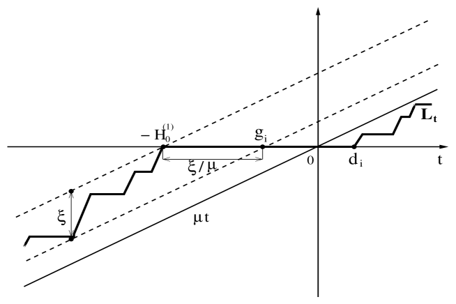
Figure 2: The on-going idle period at time zero.

5 The joint distribution of the starting and the ending times of the on-going busy and idle periods

In this section, as our main result, we compute the joint distribution of the starting time and the ending time of the busy and idle periods. We remark that it is possible to compute the joint distribution directly in the case of the idle period, but we have not been able to do this in the busy period case. To resolve this difficulty we use the theory of Palm probability and properties of a special class of two-dimensional random variables to show that it is enough to know only the Laplace transforms of $d_{b}$ (respectively, $-g_{i}$) in order to obtain the joint Laplace transforms of $d_{b}$ and $-g_{b}$ (respectively, $d_{i}$ and $-g_{i}$).

Theorem 5.1.

1) For $\alpha\neq\beta$,

$$\mathbf{E}\left(e^{\alpha g_{b}-\beta d_{b}}\,|\,S_{0}>0\right)=\frac{\alpha^{*}}{\alpha-\beta}\left(\frac{\alpha}{\eta(\alpha/\mu)}-\frac{\beta}{\eta(\beta/\mu)}\right).$$ (5.1)

2) For $\alpha\neq\beta$,

$$\mathbf{E}\left(e^{\alpha g_{i}-\beta d_{i}}\,|\,S_{0}=0\right)=\frac{\alpha^{*}\mu}{(M\mu-1)(\alpha-\beta)}\left(\frac{\psi(\alpha)}{\alpha-\alpha^{*}}-\frac{\psi(\beta)}{\beta-\alpha^{*}}\right).$$ (5.2)

Remark 5.2.

Letting $\beta\to\alpha$ in $(\ref{jointbusy})$ and $(\ref{jointidle})$ gives us the Laplace transforms of the lengths of the busy and idle periods

$$\mathbf{E}\left(e^{-\alpha(d_{b}-g_{b})}\,|\,S_{0}>0\right)=\alpha^{*}\frac{d}{d\alpha}\left(\frac{\alpha}{\eta(\alpha/\mu)}\right)$$

and

$$\mathbf{E}\left(e^{-\alpha(d_{i}-g_{i})}\,|\,S_{0}>0\right)=\frac{\alpha^{*}\mu}{M\mu-1}\frac{d}{d\alpha}\left(\frac{\psi(\alpha)}{\alpha-\alpha^{*}}\right),$$

respectively.

To prove Theorem 5.1 we use the point process approach to the storage process $S$ proposed in Mannersalo, Norros, and Salminen [9]. When $S$ hits zero it stays there for a positive amount of time a.s. Hence, we can construct from $S$ a stationary marked point process $N=\{(T_{n},Z_{n}):n\in\mathbb{Z}\}$ with a finite intensity $\lambda$, where for every $n$, $T_{n}$ and $T_{n+1}$ are the starting and ending times, respectively, of an idle or a busy period and $Z_{n}$ is the mark associated with point $T_{n}$. We let $Z_{n}=0$ if $T_{n}$ is a starting point for an idle period, otherwise $Z_{n}=1$. Let $\mathbf{P}_{N}$ and $\mathcal{F}$ denote the probability measure and the natural $\sigma$-algebra, respectively, induced by $N$. We assume that $\{T_{n}:n\in\mathbb{Z}\}$ are ordered so that $-\infty<\cdots<T_{-1}<T_{0}\leq 0<T_{1}<T_{2}<\cdots+\infty$. Let $\theta_{t}$ be the shift operator and $\mathbf{P}_{N}^{0}$ the Palm probability, which is related to the probability measure $\mathbf{P}_{N}$ via Ryll-Nardzewski and Slivnyak’s formula:

$$\mathbf{P}_{N}(A)=\lambda\int_{0}^{\infty}\mathbf{P}_{N}^{0}(T_{1}>t,\theta_{t}\in A)\,dt,\quad A\in\mathcal{F}.$$ (5.3)

Recall that the Palm probability $\mathbf{P}_{N}$ can be interpreted as the conditional probability, given that there is a point at time zero, i.e.,

$$\mathbf{P}_{N}^{0}(\{T_{0}=0\})=1.$$ (5.4)

For more details about these concepts, see Baccelli and Brémaud [1] or Mannersalo, Norros, and Salminen [9]. From relationship (5.3) we obtain now the following property of the joint distribution of $T_{0}$ and $T_{1}$.

Proposition 5.3.

For $z=0$ or $1$ and $v\geq 0,\>w\geq 0$,

$$\mathbf{P}(T_{1}>v,-T_{0}>w,\,Z_{0}=z)=\lambda\int_{v+w}^{\infty}\mathbf{P}_{N}^{0}(T_{1}>t,\,Z_{0}=z)\,dt.$$ (5.5)

Proof: To establish formula $(\ref{eqtt1})$ we only need to take $A=\{T_{1}>v,-T_{0}>w,\,Z_{0}=z\}$ in (5.3) and use that for all $t\in[0,T_{1})$,

$$Z_{0}\circ\theta_{t}=Z_{0},$$

$$T_{1}\circ\theta_{t}=T_{1}-t,$$

and

$$-T_{0}\circ\theta_{t}=t$$

$\mathbf{P}_{N}^{0}$-a.s. (for $T_{0}$, see ($\ref{eqp})$). ∎

Consider now the on-going busy period of $S$. There are obvious analogous formulas for the idle period. By (5.5), we obtain

$$\mathbf{P}(-g_{b}>v,d_{b}>w\,,\,S_{0}>0) = \mathbf{P}(T_{1}>v,-T_{0}>w\,,\,Z_{0}=1)$$ (5.6)

$$= \lambda\int_{v+w}^{\infty}\mathbf{P}_{N}^{0}(T_{1}>u\,,\,Z_{0}=1)\,du.$$

Consequently, letting

$$F_{b}^{c}(v,w):=\mathbf{P}(-g_{b}>v,d_{b}>w\,|\,S_{0}>0)$$

it is seen that

$$F_{b}^{c}(v,w)=F_{b}^{c}(v+w,0).$$ (5.7)

Two-dimensional positive random variables with the property $(\ref{fk})$ form a special class of random variables studied, e.g., in Salminen and Vallois [14]. The alternative definition of this class, denoted by $\mathcal{K}$, is as follows.

Definition 5.4.

A two-dimensional positive random variable $(X,Y)$ belongs to the class $\mathcal{K}$ if $(X,Y)$ has the same distribution as $(UV,(1-U)V)$, where the random variable $U$ has the uniform distribution on $(0,1)$, and $V$ is an arbitrary positive random variable independent of $U$.

Remark 5.5.

In reliability theory the functions with the property $(\ref{fk})$ are called Schur-constant functions (see, e.g., Bassan and Spizzichino [2]).

The next proposition describes the structure of the joint density of an element in $\mathcal{K}$ (for the proof, see Salminen and Vallois [14]).

Proposition 5.6.

Let $(X,Y)\in\mathcal{K}$ be such that there exists the density $F^{\prime}_{V}(v)=:p(v)$. Then

$$\mathbf{P}(X\in dx,Y\in dy)=f(x+y)\,dx\,dy,$$

where

$$f(v)=v^{-1}p(v),\quad v>0.$$

We have also the following characterization of elements in the class $\mathcal{K}$ in terms of the Laplace transforms.

Proposition 5.7.

Let $X$ and $Y$ be positive random variables. Then $(X,Y)\in\mathcal{K}$ if and only if there exists a positive random variable $V$ such that for all $\alpha\neq\beta$,

$$\mathbf{E}\left(e^{-\alpha X-\beta Y}\right)=\frac{1}{\alpha-\beta}\int_{\beta}^{\alpha}\mathbf{E}\left(e^{-\gamma V}\right)d\gamma.$$ (5.8)

In particular, $V\stackrel{{\scriptstyle d}}{{=}}X+Y$.

Proof: $\Rightarrow)$ Let $(X,Y)\in\mathcal{K}$. Then there exists a positive $V$ such that

$$(X,Y)\stackrel{{\scriptstyle d}}{{=}}(UV,(1-U)V),$$

where $U\sim U(0,1)$ is independent of $V$. Taking $\alpha>\beta$ we compute

$$\mathbf{E}\left(e^{-\alpha X-\beta Y}\right) = \mathbf{E}\left(e^{-\alpha UV-\beta(1-U)V}\right)$$

$$= \mathbf{E}\left(e^{-(\alpha-\beta)UV-\beta V}\right)$$

$$= \int_{0}^{\infty}\mathbf{E}\left(e^{-(\alpha-\beta)Uv-\beta v}\right)F_{V}(dv)$$

$$= \frac{1}{\alpha-\beta}\int_{0}^{\infty}\frac{e^{-\beta v}-e^{-\alpha v}}{v}F_{V}(dv)$$

$$= \frac{1}{\alpha-\beta}\int_{0}^{\infty}\left(\int_{\beta}^{\alpha}e^{-v\gamma}d\gamma\right)F_{V}(dv)$$

$$= \frac{1}{\alpha-\beta}\int_{\beta}^{\alpha}\mathbf{E}\left(e^{-\gamma V}\right)d\gamma,$$

as claimed in $(\ref{formulakl})$.
$\Leftarrow)$ Now suppose that we have a pair $(X,Y)$ of random variables such that $(\ref{formulakl})$ holds. Letting $\alpha\to\beta$ in $(\ref{formulakl})$ and using the continuity of the Laplace transforms, we get that $X+Y$ has the same law as $V$. Further, let $U\sim U(0,1)$ be independent of $V$. Then $(UV,(1-U)V)\in\mathcal{K}$ and by the sufficiency part of the proof, for $\alpha\neq\beta$,

$$\mathbf{E}\left(e^{-\alpha UV-\beta(1-U)V}\right)=\frac{1}{\alpha-\beta}\int_{\beta}^{\alpha}\mathbf{E}\left(e^{-tV}\right)dt.$$

Hence, by uniqueness of the Laplace transforms

$$(X,Y)\stackrel{{\scriptstyle d}}{{=}}(UV,(1-U)V)\in\mathcal{K}.$$

This completes the proof. ∎

Remark 5.8.

If $(X,Y)\in\mathcal{K}$ and the Laplace transform of $X$ is known, we can easily compute the joint Laplace transform. Indeed, denote $I(\alpha):=\int_{0}^{\alpha}\mathbf{E}\left(e^{-\gamma V}\right)d\gamma$. Then setting $\beta=0$ in formula $(\ref{formulakl})$, we get

$$\mathbf{E}\left(e^{-\alpha X}\right)=\frac{1}{\alpha}I(\alpha)$$

and hence,

$$\mathbf{E}\left(e^{-\alpha X-\beta Y}\right) = \frac{1}{\alpha-\beta}\int_{\beta}^{\alpha}\mathbf{E}\left(e^{-\gamma V}\right)d\gamma$$

$$= \frac{1}{\alpha-\beta}\left(I(\alpha)-I(\beta)\right).$$

We conclude now the proof of Theorem 5.1. By $(\ref{eqtt1})$, the two-dimensional random variable $(-g_{b},d_{b})\in\mathcal{K}$ and the marginal Laplace transform of $d_{b}$ is given by $(\ref{formula1})$. Hence we can use Remark 5.8 to get the joint distribution of $-g_{b}$ and $d_{b}$. From Theorem 3.1 we have

$$\mathbf{E}(e^{-\alpha d_{b}}\,|\,S_{0}>0)=\frac{\alpha^{*}}{\eta(\alpha/\mu)}.$$

Therefore, the joint Laplace transform of $-g_{b}$ and $d_{b}$ is

$$\mathbf{E}(e^{\alpha g_{b}-\beta d_{b}}\,|\,S_{0}>0)=\frac{\alpha^{*}}{\alpha-\beta}\left(\frac{\alpha}{\eta(\alpha/\mu)}-\frac{\beta}{\eta(\beta/\mu)}\right).$$

The corresponding formula for $(-g_{i},d_{i})$ is obtained similarly. The proof of Theorem 5.1 is now complete.

6 Example: reflected Brownian motion with negative drift

Let $Z=\{Z_{t}:t\in\mathbb{R}\}$ be a reflected Brownian motion with drift $-c<0$ in stationary state living on $I=[0,\infty)$. Let

$$S_{t}:=\sup_{s\leq t}\{L_{t}-L_{s}-(t-s)\}$$

be the local time storage process (as introduced in Section 2), associated with $Z$. In this case we have

$$m(dx)=2e^{-2cx}dx,$$

and $M:=m\{I\}=1/c$. The storage process $S$ is well-defined if and only if $0<c<1$. For a reflected Brownian motion with drift $-c$ the Green function at $(0,0)$ is

$$G_{\alpha}(0,0)=\frac{1}{\sqrt{2\alpha+c^{2}}-c},$$

and the function $\psi$ (cf. (2.4)) takes the form

$$\psi(\alpha)=\alpha-\sqrt{2\alpha+c^{2}}+c,\quad\alpha\geq 0$$

Hence,

$$\alpha^{*}=2(1-c)$$

and

$$\eta(\alpha)=\alpha+1-c+\sqrt{2\alpha+(1-c)^{2}}.$$

Using $(\ref{jointbusy})$, we compute

$$\mathbf{E}\left(e^{\alpha g_{b}-\beta d_{b}}\,|\,S_{0}>0\right)$$

$$\hskip 5.69046pt=\frac{2(1-c)}{\alpha-\beta}\left(\frac{\alpha}{\alpha+1-c+\sqrt{2\alpha+(1-c)^{2}}}-\frac{\beta}{\beta+1-c+\sqrt{2\beta+(1-c)^{2}}}\right)$$

$$\hskip 5.69046pt=\frac{1}{\alpha-\beta}\left(\frac{4(1-c)}{\sqrt{2\beta+(1-c)^{2}}+1+c}-\frac{4(1-c)}{\sqrt{2\alpha+(1-c)^{2}}+1+c}\right)$$

$$\hskip 5.69046pt=\frac{8(1-c)}{\sqrt{2\alpha+(1-c)^{2}}+\sqrt{2\beta+(1-c)^{2}}}$$

$$\hskip 42.67912pt\times\frac{1}{(\sqrt{2\alpha+(1-c)^{2}}+1+c)(\sqrt{2\beta+(1-c)^{2}}+1+c)}$$

$$\hskip 5.69046pt=:F(\alpha,\beta;1-c).$$ (6.1)

For the on-going idle period at zero, using $(\ref{jointidle})$, we obtain after some cancellations that

$$\mathbf{E}\left(e^{\alpha g_{i}-\beta d_{i}}\,|\,S_{0}>0\right)=F(\alpha,\beta;c).$$

This formula can also be found in [9] but $(\ref{busybrown})$ is a new result.

To find the joint density of $(-g_{b},d_{b})$, given that $S_{0}>0$, first find the density of $V:=-g_{b}+d_{b}$, given that $S_{0}>0$. Setting $\beta=\alpha$ in the right-hand side of $(\ref{busybrown})$, we get

$$\mathbf{E}\left(e^{-\alpha(d_{b}-g_{b})}\,|\,S_{0}>0\right)=\frac{4(1-c)}{\sqrt{2\alpha+(1-c)^{2}}(\sqrt{2\alpha+(1-c)^{2}}+1+c)^{2}}.$$ (6.2)

Taking the inverse Laplace transform of $(\ref{lapv})$ (cf. Erd lyi [6], p. 234) we obtain the density of the length of the busy period $d_{b}-g_{b}$, given that $S_{0}>0$, as

$$p_{c}(v)=2(1-c)\sqrt{\frac{2v}{\pi}}e^{-\frac{(1-c)^{2}}{2}v}-4(1-c^{2})ve^{2cv}\Phi\left(-\frac{1+c}{2}\sqrt{v}\right),\;v>0,$$

where $\Phi(v)$ is the standard normal distribution function. Note that the density of the length of the idle period $d_{i}-g_{i}$, given that $S_{0}=0$, is $p_{1-c}(v),\,v>0$. Using Proposition 5.6, we get the joint density of the starting and the ending points of the busy period as

$$\mathbf{P}(-g_{b}\in dx,d_{b}\in dy\,|\,S_{0}>0)$$

$$\hskip 19.91684pt=2(1-c)\sqrt{\frac{2}{\pi(x+y)}}e^{-\frac{(1-c)^{2}}{2}(x+y)}$$

$$\hskip 34.14322pt-4(1-c^{2})e^{2c(x+y)}\Phi\left(-\frac{1+c}{2}\sqrt{x+y}\right)\,dx\,dy.$$

Acknowledgements

The authors thank Ilkka Norros for a short but stimulating discussion, and Bruno Bassan and Fabio Spizzichino for pointing out the connection of the class $\mathcal{K}$ and the Schur-constant functions.

References

[1]
F. Baccelli and P. Brémaud.
Elements of Queueing Theory. Second edition.
Springer Verlag, Berlin Heidelberg New York, 2003.
[2]
B. Bassan and F. Spizzichino.
Stochastic comparisons for residual lifetimes and bayesian notions of
multivariate ageing.
Adv. Appl. Prob., 31:1078–1094, 1999.
[3]
J. Bertoin.
Sur la décomposition de la trajectoire d’un processus de Lévy
spectralement positif en son minimum.
Ann. Inst. Henri Poincaré, 27(4):537–548, 1991.
[4]
N.H. Bingham.
Fluctuation theory in continuous time.
Adv. in Appl. Probab., 7:705–766, 1975.
[5]
A.N. Borodin and P. Salminen.
Handbook of Brownian Motion – Facts and Formulae, 2nd
edition.
Birkhäuser, Basel, Boston, Berlin, 2002.
[6]
A. Erdélyi.
Tables of Integral Transforms.
McGraw-Hill, New York, 1954.
[7]
J.M. Harrison.
Brownian Motion and Stochastic Flow Systems.
Wiley, New York, 1985.
[8]
K. Itô and H.P. McKean.
Diffusion Processes and Their Sample Paths.
Springer Verlag, Berlin, Heidelberg, 1974.
[9]
P. Mannersalo, I. Norros, and P. Salminen.
A storage process with local time input.
To appear in Queueing Systems, 2003.
[10]
N. U. Prabhu.
Stochastic Storage Processes.
Springer Verlag, New York, Berlin, Heidelberg, 1998.
2nd edition.
[11]
E. Reich.
On the integrodifferential equation of Takács I.
Annals of Mathematical Statistics, 29:563–570, 1958.
[12]
J. Roberts, U. Mocci, and J. Virtamo, editors.
Broadband Network Teletraffic.
Number 1155 in Lecture Notes in Computer Science. Springer, 1996.
[13]
P. Salminen.
On the distribution of diffusion local time.
Statistics and Probability Letters, 18:219–225, 1993.
[14]
P. Salminen and P. Vallois.
On first range times for linear diffusions.
To appear in J. Theoretical Probab.