Collision Free Motion Planning on Graphs

Abstract.

A topological theory initiated in [4], [5] uses methods of algebraic topology to estimate numerically the character of instabilities arising in motion planning algorithms. The present paper studies random motion planning algorithms and reveals how the topology of the robot’s configuration space influences their structure. We prove that the topological complexity of motion planning ${\rm\bf{TC}}(X)$ coincides with the minimal $n$ such that there exists an $n$-valued random motion planning algorithm for the system; here $X$ denotes the configuration space. We study in detail the problem of collision free motion of several objects on a graph $\Gamma$. We describe an explicit motion planning algorithm for this problem. We prove that if $\Gamma$ is a tree and if the number of objects is large enough, then the topological complexity of this motion planning problem equals $2m(\Gamma)+1$ where $m(\Gamma)$ is the number of the essential vertices of $\Gamma$. It turns out (in contrast with the results on the collision free control of many objects in space [7]) that the topological complexity is independent of the number of particles.

1. Introduction

Algorithmic motion planning in robotics is a well established discipline which provides (1) a wide variety of general-purpose efficient theoretical algorithms, (2) more efficient algorithms designed for a number of special situations and (3) some practical solutions which work reasonably well in fairly involved scenarios. We refer to [14] for a recent survey and to [11] for a comprehensive textbook.

In general, one is given a moving system $R$ with $k$ degrees of freedom and a two or three-dimensional workspace $V$. The geometry of $R$ and of $V$ is given in advance which determines the configuration space of the system, $X$. The latter is a subset of $\mathbf{R}^{k}$ consisting of all placements (or configurations) of the system $R$, each represented by a tuple of $k$ real parameters, such that in this placement $R$ lies fully in $V$. For simplicity we may restrict our attention to a single connected component of $R$, the one containing a prescribed initial placement of $R$.

Being a subset of the Euclidean space $\mathbf{R}^{k}$, the configuration space $X$ naturally inherits its topology. Many questions of control theory depend solely on the configuration space $X$ viewed as a topological space. One of the advantages of this approach is that different control problems could be treated simultaneously for all systems having homeomorphic configuration spaces. It is well-known that any real analytic manifold can be realized as the configuration space of a simple mechanical system (linkage). Therefore topological questions of robotics lead to interesting new topological invariants of abstract manifolds.

We are interested in motion planning algorithms which work as follows: the algorithm gets as its input the present and the desired states of the system and it produces as the output a continuous motion of the system from its current state to the desired state. It turns out that the topology of the configuration space of the system imposes important restrictions on the discontinuities of the robot motion as a function of the input data. We emphasize that these are not discontinuities of the robot motion as a function of time. The discontinuities which we study here are in the way the decision (the whole motion) depends on the input data.

The approach to the motion planning problem described in [4], [5] was initially inspired by my discussions with Dan Halperin and Micha Sharir in 2000. It was also influenced by the well-known previous work of S. Smale [15] on algorithms of finding roots of algebraic equations.

Our results on topological robotics were published in mathematical journals [4], [5], [6] and in [7]. They led to an interesting new topological invariant ${\rm\bf{TC}}(X)$ of topological spaces. In robotics applications, the number ${\rm\bf{TC}}(X)$ has at least three different appearances. Firstly, it is the minimal number of domains of continuity of any motion planning algorithm for a system having $X$ as its configuration space. Secondly, it is the minimal order of instability (see [5]) which have motion planning algorithms in $X$. The third interpretation (see §6 below) allows to measure ${\rm\bf{TC}}(X)$ while relying on random motion planning algorithms: we show that ${\rm\bf{TC}}(X)$ is the minimal integer $n$ such that there exists an $n$ valued random motion planning algorithm for the system.

The main part of the paper is devoted to a very specific motion planning problem: simultaneous control of many objects whose motion is restricted by a graph and the goal is to construct a motion planning algorithm avoiding collisions between the objects. This problem was initially studied by R. Ghrist, D. Koditschek and A. Abrams [8], [9], [1]. We calculate here the topological complexity of the problem and describe an explicit motion planning algorithm solving it.

For convenience of the reader we have included sections §§2 - 5 which give a brief description of some results of [4], [5] used later in this paper.

2. Motion Planning Algorithms

Consider a mechanical system (robot) controlled by a motion planning algorithm. It is supposed to function as follows: an operator introduces into the computer of the system the current and the desired states of the system and the motion planning algorithm determines a continuous motion of the system from its current state to the desired state.

Let $X$ be the configuration space of the system. We will always assume that $X$ is path connected, i.e. any pair of points $A,B\in X$ may be joined by a continuous path $\gamma$ in $X$. This means that it is possible to bring our system, by a continuous movement, from any given configuration $A$ to any given configuration $B$. This assumption does not represent a restriction since in practical situations when the natural configuration space of a given system has several connected components, we may simply restrict our attention to one of them.

Given two points $A,B\in X$, one wants to connect them by a path in $X$; this path represents a continuous motion of the system from one state to the other. A motion planning algorithm is a rule (algorithm) that takes pairs of configurations $(A,B)\in X\times X$ as an input and produces a continuous path in $X$ from $A$ to $B$ as an output.

Let $PX$ denote the space of all continuous paths $\gamma:[0,1]\to X$, equipped with the compact-open topology, and let $\pi:PX\to X\times X$ be the map assigning the end points to a path: $\pi(\gamma)=(\gamma(0),\gamma(1))$. Rephrasing the above discussion we see that a motion planning algorithm is a section of this fibration

(1) $$s:X\times X\to PX,\quad\pi\circ s=1_{X\times X}.$$

Here $1_{X\times X}:X\times X\to X\times X$ denotes the identity map. The algorithm associates the curve $s(A,B)(t)$, where $t\in[0,1]$, with any two given configurations of the system $A,B\in X$.

Given a mechanical system, one asks does there exist a continuous motion planning algorithm for it? In other words, whether it is possible to find a continuous section (1). The answer is negative in most cases as the following theorem proven in [4] states:

Theorem 1.

A globally defined continuous motion planning algorithm (1) exists if and only if the configuration space $X$ of the system is contractible.

3. Topological Complexity of Motion Planning Algorithms

In view of Theorem 1, one expects that in general a motion planning algorithm is only piecewise continuous. The following definition describes an important class of piecewise continuous motion planning algorithms having finitely many domains of continuity:

Definition 1.

Let $X$ be a path-connected topological space. A motion planning algorithm (1) is called tame if there exist finitely many subsets

(2) $$F_{1},\dots,F_{k}\subset X\times X$$

such that the following conditions are satisfied:

1. the sets $F_{1},\dots,F_{k}$ are pairwise disjoint $F_{i}\cap F_{j}=\emptyset$, $i\not=j$, and cover $X\times X$, i.e. $X\times X=F_{1}\cup F_{2}\cup\dots\cup F_{k};$

2. each restriction $s|_{F_{j}}$ is continuous;

3. each set $F_{j}$ is an ENR (see below).

Condition (a) means that the sets $F_{1},\dots,F_{k}$ partition the total space of all possible pairs $X\times X$. Condition (b) is the major continuity assumption. Condition (c) is technical, it allows to avoid pathological (exotic) decompositions. Recall, a topological space $Y$ is called an Euclidean Neighborhood Retract (ENR) if it is homeomorphic to a subset of a Euclidean space $Y^{\prime}\subset{\mathbf{R}}^{n}$, such that $Y^{\prime}$ is a retract of some open neighborhood $Y^{\prime}\subset U\subset{\mathbf{R}}^{n}$; in other words, $U\subset{\mathbf{R}}^{n}$ is open and there exists a continuous map $r:U\to Y^{\prime}$ such that $r(y)=y$ for all $y\in Y^{\prime}$. Such a continuous map $r$ is called a retraction.

It is well-known that all manifolds and polyhedra are ENRs.

For a given algorithm (1) there may exist many different decompositions (2) satisfying the conditions of Definition 1.

Definition 2.

The topological complexity of a tame motion planning algorithm $s:X\times X\to PX$, $\pi\circ s=1_{X\times X}$ is defined as the minimal number $k$ of domains of continuity $F_{j}$ which appear in Definition 1.

Given a concrete mechanical system one wishes to construct motion planning algorithms for it with the minimal possible topological complexity. The problem clearly depends only on the topology of the configuration space $X$ of the system. This leads to the following purely topological notion:

Definition 3.

Let $X$ be a path-connected topological space. The topological complexity of $X$ is defined as the minimal topological complexity of motion planning algorithms in $X$.

The topological complexity of a topological space $X$ coincides (for nice spaces $X$) with the invariant ${\rm\bf{TC}}(X)$ which was introduced in [4]. Its definition (which is more convenient from the purely topological point of view) appears in the following section.

4. Topological Invariant ${\rm\bf{TC}}(X)$

Definition 4.

Let $X$ be a path-connected topological space. The number ${\rm\bf{TC}}(X)$ is defined as the minimal integer $r$ such that the Cartesian product $X\times X$ can be covered by $r$ open subsets

(3) $$X\times X=U_{1}\cup U_{2}\cup\dots\cup U_{r},$$

such that for any $i=1,2,\dots,r$ there exists a continuous map

(4) $$s_{i}:U_{i}\to PX\quad\mbox{with}\quad\pi\circ s_{i}=1_{U_{i}}.$$

If no such $r$ exists, we set ${\rm\bf{TC}}(X)=\infty$.

It is shown in [4] that ${\rm\bf{TC}}(X)$ depends only on the homotopy type of $X$.

The invariant ${\rm\bf{TC}}(X)$ admits an upper bound [4]:

(5) $${\rm\bf{TC}}(X)\leq 2\dim X+1.$$

The number ${\rm\bf{TC}}(X)$ was computed in [4],[5],[6], [7] for a number of important configuration spaces appearing in robotics.

Theorem 2.

Let $X$ be a connected smooth manifold. Then the topological complexity of $X$ (cf. Definition 3) coincided with ${\rm\bf{TC}}(X)$ (cf. Definition 4).

We refer to [5] for a proof.

A lower bound for ${\rm\bf{TC}}(X)$ is based on the knowledge of the cohomology algebra of $X$. To describe this result (which will be used later in this paper) we first observe that the singular cohomology $H^{\ast}(X;{\mathbf{R}})=H^{\ast}(X)$ is a graded ${\mathbf{R}}$-algebra with the multiplication

(6) $$\cup:H^{\ast}(X)\otimes H^{\ast}(X)\to H^{\ast}(X)$$

given by the cup-product, see [3], [16]. The tensor product $H^{\ast}(X)\otimes H^{\ast}(X)$ is again a graded ${\mathbf{R}}$-algebra with the multiplication

(7) $$(u_{1}\otimes v_{1})\cdot(u_{2}\otimes v_{2})=(-1)^{|v_{1}|\cdot|u_{2}|}\,u_{1}u_{2}\otimes v_{1}v_{2}.$$

Here $|v_{1}|$ and $|u_{2}|$ denote the degrees of cohomology classes $v_{1}$ and $u_{2}$ correspondingly. The cup-product (6) is an algebra homomorphism.

Definition 5.

The kernel of homomorphism (6) is called the ideal of the zero-divisors of $H^{\ast}(X)$. The zero-divisors-cup-length of $H^{\ast}(X)$ is the length of the longest nontrivial product in the ideal of the zero-divisors of $H^{\ast}(X)$.

The next result is the main cohomological lower bound for the topological complexity.

Theorem 3.

${\rm\bf{TC}}(X)$ is greater than the zero-divisors-cup-length of the cohomology algebra $H^{\ast}(X)$.

See [4] for a proof.

As an illustration we state the following result from [5] which is relevant for the sequel:

Theorem 4.

Let $X$ be a connected graph. Then

(11) $${\rm\bf{TC}}(X)=\left\{\begin{array}[]{lll}1,&\mbox{if}&b_{1}(X)=0,\\ 2,&\mbox{if}&b_{1}(X)=1,\\ 3,&\mbox{if}&b_{1}(X)\geq 2.\end{array}\right.$$

Here $b_{1}(X)$ denotes the first Betti number of $X$.

5. Order of Instability

Besides the number of domains of continuity, the motion planning algorithms could be characterized by their orders of instability.

Let $s:X\times X\to PX$, $\pi\circ s=1_{X\times X}$ be a tame motion planning algorithm (cf. Definition 1). Let $F_{1},\dots,F_{k}\subset X\times X$ be pairwise disjoint subsets as in Definition 1, i.e. such that $s|_{F_{j}}$ is continuous, each $F_{j}$ is an ENR and union of the sets $F_{j}$ equals $X\times X$.

Definition 6.

The order of instability of a motion planning algorithm $s$ is defined as the smallest integer $r$ such that the subsets $F_{1},\dots,F_{k}\subset X\times X$ as above could be constructed in such a way that for any sequence of $r+1$ indices $1\leq i_{1}<i_{2}<\dots<i_{r+1}\leq k$ one has

(12) $$\bar{F}_{i_{1}}\cap\bar{F}_{i_{2}}\cap\dots\cap\bar{F}_{i_{r+1}}=\emptyset.$$

Here $\bar{F}_{j}$ denotes the closure of $F_{j}$ in $X\times X$.

The order of instability represents a very important functional characteristic of a motion planning algorithm. If the order of instability equals $r$ then there exists a pair of initial - final configurations $(A,B)\in F_{j}$ such that arbitrarily close to $(A,B)$ there exist $r-1$ pairs of configurations $(A_{1},B_{1})$, $(A_{2},B_{2})$, $\dots$, $(A_{r-1},B_{r-1})$ (which are all distinct small perturbations of $(A,B)$), belonging to distinct sets $F_{i}$, $i\not=j$. This means that small perturbations of the input data $(A,B)$ may lead to $r$ essentially distinct motions given by the motion planning algorithm $s$.

In practical situations one prefers to have motion planning algorithms with order of instability as low as possible.

Theorem 5.

Let $X$ be a connected smooth manifold. Then the order of instability of any tame motion planning algorithm (1) is at least ${\rm\bf{TC}}(X)$. Moreover, there exists a motion planning algorithm with the order of instability ${\rm\bf{TC}}(X)$.

This theorem proven in [5] gives yet another way the topological invariant ${\rm\bf{TC}}(X)$ appears in robotics. In the next section we explain how the topological quantity ${\rm\bf{TC}}(X)$ shows in random algorithms.

6. Random Motion Planning Algorithms

According to Theorem 1, deterministic continuous motion planning algorithms $s:X\times X\to PX$ exist only when the configuration space $X$ is contractible. Instead, one may work with random algorithms solving the motion planning problem.

Let $X$ be a path-connected topological space. A random $n$-valued path $\sigma$ in $X$ starting at $A\in X$ and ending at $B\in X$ is given by an ordered sequence of paths $\gamma_{1},\dots,\gamma_{n}\in PX$ and an ordered sequence of real numbers $p_{1},\dots,p_{n}\in[0,1]$ such that each $\gamma_{j}:[0,1]\to X$ is a continuous path in $X$ starting at $A=\gamma_{j}(0)$ and ending at $B=\gamma_{j}(1)$, and

$$p_{j}\geq 0,\quad p_{1}+p_{2}+\dots+p_{n}=1.$$

One thinks of the paths $\gamma_{1},\dots,\gamma_{n}$ as of the states of $\sigma$ and of the number $p_{j}$ as being the probability that the random path $\sigma$ is in state $\gamma_{j}$. Random path $\sigma$ as above will be written as a formal linear combination

(13) $$\sigma=p_{1}\gamma_{1}+p_{2}\gamma_{2}+\dots+p_{n}\gamma_{n}.$$

Equality between $n$-valued random paths is understood as follows: the random path (13) is equivalent to $\sigma^{\prime}=p^{\prime}_{1}\gamma^{\prime}_{1}+p^{\prime}_{2}\gamma^{\prime}_{2}+\dots+p^{\prime}_{n}\gamma^{\prime}_{n}$ iff $p_{j}=p^{\prime}_{j}$ for all $j=1,\dots,n$ and, besides, $\gamma_{j}=\gamma^{\prime}_{j}$ for all indices $j$ with $p_{j}\not=0$. In other words the path $\gamma_{j}$ which appears with the zero probability $p_{j}=0$ could be replaced by any other path starting at $A$ and ending at $B$.

We denote by $P_{n}X$ the space of all $n$-valued random paths in $X$. The space $P_{n}X$ has a natural topology: it is a factor-space of a subspace of the Cartesian product of $n$ copies of $PX\times[0,1]$. Note that the space $P_{1}X$ coincides with $PX$. The canonical map

(14) $$\pi:P_{n}X\to X\times X$$

assigns to a random path its initial and end points. Map (14) is continuous.

Definition 7.

An $n$-valued random motion planning algorithm is defined as a continuous map

(15) $$s:X\times X\to P_{n}X$$

such that $\pi\circ s=1_{X\times X}$.

Given a pair $(A,B)\in X\times X$, the output of the algorithm

(16) $$s(A,B)=p_{1}\gamma_{1}+\dots+p_{n}\gamma_{n}$$

is an ordered probability distribution on the paths between $A$ and $B$. In other words, the algorithm $s$ produces the motion $\gamma_{j}$ with probability $p_{j}$ where $j=1,\dots,n$.

Theorem 6.

Let $X$ be a path-connected metric space. Then the minimal integer $n$ such that there exists an $n$-valued random motion planning algorithm $s:X\times X\to P_{n}X$ in $X$ coincides with ${\rm\bf{TC}}(X)$.

Proof.

The following proof is an adjustment of the proof of Proposition 2 from [13]. Assume that there exists an $n$-valued random motion planning algorithm $s:X\times X\to P_{n}X$ in $X$. The right hand side of formula (16) defines continuous real valued functions $p_{j}:X\times X\to[0,1]$, where $j=1,\dots,n$. Let $U_{j}$ denote the open set $p_{j}^{-1}(0,1]\subset X\times X$. The sets $U_{1},\dots,U_{n}$ form an open covering of $X\times X$. Setting $s_{j}(A,B)=\gamma_{j}$, one gets a continuous map $s_{j}:U_{j}\to PX$ with $\pi\circ s_{i}=1_{U_{j}}$. Hence, $n\geq{\rm\bf{TC}}(X)$ according to the definition of ${\rm\bf{TC}}(X)$.

Conversely, setting $k={\rm\bf{TC}}(X)$, we obtain that there exists an open cover $U_{1},\dots,U_{k}\subset X\times X$ and a sequence of continuous maps $s_{i}:U_{i}\to PX$ where $\pi\circ s_{i}=1_{U_{i}}$, $i=1,\dots,k$. Extend $s_{i}$ to an arbitrary (possibly discontinuous) mapping

$$S_{i}:X\times X\to PX$$

satisfying $\pi\circ S_{i}=1_{X\times X}$. This can be done without any difficulty; it amounts in making a choice of a connecting path for any pair of points $(A,B)\in X\times X-U_{i}$. Next, one may find a continuous partition of unity subordinate to the open cover $U_{1},\dots,U_{k}$. It is a sequence of continuous functions $p_{1},\dots,p_{k}:X\times X\to[0,1]$ such that for any pair $(A,B)\in X\times X$ one has

$$p_{1}(A,B)+p_{2}(A,B)+\dots+p_{k}(A,B)=1$$

and the closure of the set $p_{i}^{-1}(0,1]$ is contained in $U_{i}$. We obtain a continuous $k$-valued random motion planning algorithm $s:X\times X\to P_{n}X$ given by the following explicit formula

(17) $$s(A,B)=p_{1}(A,B)S_{1}(A,B)+\dots+p_{k}(A,B)S_{k}(A,B).$$

The continuity of $s$ follows from the continuity of the maps $S_{i}$ restricted to the domains $p_{i}^{-1}(0,1]$. This completes the proof. ∎

7. Configuration Spaces of Graphs

Let $\Gamma$ be a connected finite graph. The symbol $F(\Gamma,n)$ denotes the configuration space of $n$ distinct particles on $\Gamma$. In other words, $F(\Gamma,n)$ is the subset of the Cartesian product

$$\underbrace{\Gamma\times\Gamma\times\dots\times\Gamma}_{n\,\,\mbox{\scriptsize times}}=\Gamma^{\times n}$$

consisting of configurations $(x_{1},x_{2},\dots,x_{n})$ where $x_{i}\in\Gamma$ and $x_{i}\not=x_{j}$ for $i\not=j$. The topology of $F(\Gamma,n)$ is induced from its embedding into $\Gamma^{\times n}$.

Configuration spaces of graphs were studied by R. Ghrist, D. Koditschek and A. Abrams, see [8], [9], [1].

To illustrate the importance of these configuration spaces for robotics one may mention the control problems where a number of automated guided vehicles (AGV) have to move along a network of floor wires [9]. The motion of the vehicles must be safe: it should be organized so that the collisions do not occur. If $n$ is the number of AGV then the natural configuration space of this problem is $F(\Gamma,n)$ where $\Gamma$ is a graph. Here we idealize reality by assuming that the vehicles have size 0 (i.e. they are points). Although this assumption simplifies our discussion, it is in fact irrelevant for the topological problems which we study.

The first question to ask is whether the configuration space $F(\Gamma,n)$ is connected. Clearly $F(\Gamma,n)$ is disconnected if $\Gamma=[0,1]$ is a closed interval (and $n\geq 2$) or if $\Gamma=S^{1}$ is the circle and $n\geq 3$. These are the only examples of this kind as the following simple lemma claims:

Lemma 7.

Let $\Gamma$ be a connected finite graph having at least one essential vertex Then the configuration space $F(\Gamma,n)$ is connected.

An essential vertex is a vertex which is incident to 3 or more edges.

One of the main results of topological robotics states that the configuration spaces $F(\Gamma,n)$ are aspherical; see [8].

For the topological complexity of the configuration spaces one has:

Theorem 8.

Let $\Gamma$ be a connected graph having an essential vertex. Then the topological complexity of $F(\Gamma,n)$ satisfies

(18) $${\rm\bf{TC}}(F(\Gamma,n))\leq 2m(\Gamma)+1,$$

where $m(\Gamma)$ denotes the number of essential vertices in $\Gamma$.

Proof.

By a theorem of R. Ghrist [8], the configuration space $F(\Gamma,n)$ has homotopy type of a cell complex of dimension $\leq m(\Gamma)$. Combining this result with the theorem about the homotopy invariance of ${\rm\bf{TC}}(X)$ (see Theorem 3 in [4]) and the with the upper bound (5) one gets (18). ∎

We prove below that equality holds in (18) in many cases.

We shall also see examples where (18) holds as a strict inequality.

8. A Motion Planning Algorithm in $F(\Gamma,n)$

In this section $\Gamma$ denotes a tree having an essential vertex.

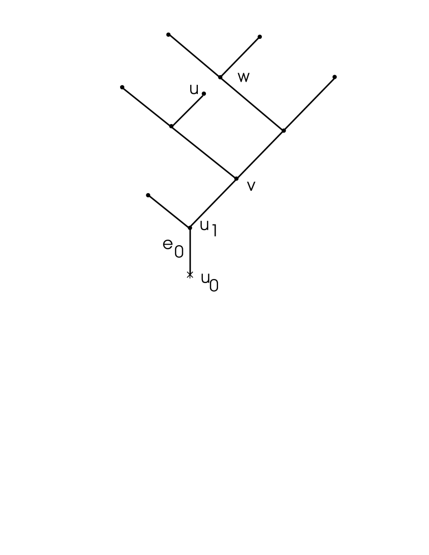
Figure 1. A partial order between the points of the tree.

Fix a univalent vertex $u_{0}\in\Gamma$ which will be called the root. Any point in $\Gamma$ can be connected by a path to the root $u_{0}$ and this connecting path is unique up to homotopy. The choice of the root determines a partial order on $\Gamma$: we say that $x\succ y$, where $x,y\in\Gamma$ if any path from $x$ to the root $u_{0}$ passes through $y$. Of course, $\succ$ is only a partial order, i.e. there may exist pairs $x,y\in\Gamma$ such that neither $x\succ y$, nor $y\succ x$. On Figure 1 we see $u\succ v$ and $w\succ v$ however the points $u$ and $w$ are not comparable.

Let $e_{0}\subset\Gamma$ denote the root edge of $\Gamma$.

Fix a configuration $\alpha_{0}\in F(\Gamma,n)$ of $n$ distinct points lying on $e_{0}$ and a continuous collision free motion connecting (in $F(\Gamma,n)$) any pair of permutations of $\alpha_{0}$. Such motions exist as we assume that $\Gamma$ has an essential vertex and hence the configuration space $F(\Gamma,n)$ is connected (see Lemma 7).

The algorithm works as follows. Let $\alpha=(A_{1},A_{2},\dots,A_{n})\in F(\Gamma,n)$ and $\beta=(B_{1},B_{2},\dots,B_{n})\in F(\Gamma,n)$ be two given configurations of $n$ distinct points on $\Gamma$. Let $A_{i_{1}},\dots,A_{i_{r}}$ be all the minimal elements (with respect to the order $\succ$) of the set of points of $\alpha$. Here the notation is such that $i_{1}<i_{2}<\dots<i_{r}$. First we move the point $A_{i_{1}}$ down to an interior point of the root edge $e_{0}$. Next we move $A_{i_{2}}$ to the root edge $e_{0}$ and we continue moving similarly the following points $A_{i_{3}},\dots,A_{i_{r}}$.

As a result, after this first stage of the algorithm, all the minimal points of $\alpha$ are transferred onto the root edge $e_{0}$. On the second stage we find the minimal set among the remaining points of $\alpha$ and move them down, one after another, to the edge $e_{0}$. Repeating in this way we find continuous collision free motion of all the points of $\alpha$ moving them onto the interior of the root edge $e_{0}$. We obtain a configuration of points $\alpha^{\prime}=(A_{1}^{\prime},\dots,A^{\prime}_{n})$ which all lie in the interior of the root edge $e_{0}$, in certain order.

For points lying on the root edge $e_{0}$ the partial order $\succ$ is a linear order. Given a configuration $A=(A_{1},\dots,A_{n})$ where all points $A_{i}$ lie on the edge $e_{0}$, there exists a unique permutation $\alpha:\{1,\dots,n\}\to\{1,\dots,n\}$ such that $A_{\alpha_{n}}\succ A_{\alpha_{n-1}}\succ\dots\succ A_{\alpha_{1}}.$ This permutation describes the order of the points on the edge. It is obvious that any two configurations having the same permutation can be connected by a continuous collision free path such that no points leave $e_{0}$ in the process of motion.

Applying the similar procedure to configuration $\beta$ we obtain a configuration $\beta^{\prime}=(B^{\prime}_{1},\dots,B^{\prime}_{n})\in F(\Gamma,n)$ connected to $\beta$ by a continuous collision free motion, such that $B^{\prime}_{i}\in{\rm{Int}}(e_{0})$ for all $j=1,\dots,n$.

Next we apply one of the precomputed permutational motions which takes $\alpha^{\prime}$ to a configuration $\alpha^{\prime\prime}$ which also lies in the interior of $e_{0}$ and has the same order as the configuration $\beta^{\prime}$.

Finally, the output of the algorithm is the concatenation of (1) the motion from $\alpha$ to $\alpha^{\prime}$; (2) the motion from $\alpha^{\prime}$ to $\alpha^{\prime\prime}$; (3) the obvious motion from $\alpha^{\prime\prime}$ to $\beta^{\prime}$; and (4) the reverse of the motion $\beta\to\beta^{\prime}$. The motion (3) exists since both $\alpha^{\prime\prime}$ and $\beta^{\prime}$ lie on $e_{0}$ and have the same order.

The above algorithm is discontinuous: if one of the points $A_{j}$ is a vertex then a small perturbation of $A_{j}$ may lead to a different set of minimal points and hence to a completely different motion. Note that the vertices of $T$ which have valence one or two do not cause discontinuity.

Let $S_{i}\subset F(\Gamma,2)$ denote the set of all configurations $\alpha=(A_{1},\dots,A_{n})$ such that precisely $i$ points among $A_{j}$ are essential vertices of $\Gamma$. If we restrict the above algorithm on the pairs $(A,B)\in S_{i}\times S_{j}$ then the result is a continuous function of the input. The sets $S_{i}\times S_{j}$ and $S_{i+1}\times S_{j-1}$ are disjoint and each of the sets contain no limit points of the other. This follows since the closure of $S_{i}$ is contained in the union of the sets $S_{j}$ with $j\geq i$. We may define

$$Y_{k}=\bigcup_{i+j=k}S_{i}\times S_{j},\quad k=0,1,\dots,2m(\Gamma)$$

where $m(\Gamma)$ denotes the number of the essential vertices of $\Gamma$. The algorithm described above is continuous when restricted on each set $Y_{k}$. Hence we obtain:

Corollary 9.

The topological complexity of the algorithm described above is less than or equal to $2m(\Gamma)+1$ where $m(\Gamma)$ denotes the number of the essential vertices of $\Gamma$.

9. The Main Result

Our main result which will be proven later in this paper states:

Theorem 10.

Let $\Gamma$ be a tree having an essential vertex. Let $n$ be an integer satisfying $n\geq 2m(\Gamma)$ where $m(\Gamma)$ denotes the number of essential vertices of $\Gamma$. In the case $n=2$ we will additionally assume that the tree $\Gamma$ is not homeomorphic to the letter $Y$ viewed as a subset of the plane $\mathbf{R}^{2}$. Then the upper bound (18) is exact, i.e.

(19) $${\rm\bf{TC}}(F(\Gamma,n))=2m(\Gamma)+1.$$

We conjecture that this theorem holds for any connected graph $\Gamma$ having $\geq 2$ essential vertices without assuming that $\Gamma$ is a tree and for any number of particles $n\geq 2m(\Gamma)$.

If $\Gamma$ is homeomorphic to the letter $Y$ then $m(\Gamma)=1$ and $F(\Gamma,2)$ is homotopy equivalent to the circle $S^{1}$. Hence in this case ${\rm\bf{TC}}(F(\Gamma,2))=2$, see [4]. The equality (19) fails in this case.

From Theorem 12 of the next section and Theorem 4 it follows that for any tree $\Gamma$ one has

(23) $${\rm\bf{TC}}(F(\Gamma,2))=\left\{\begin{array}[]{ll}2,&\,\mbox{if $\Gamma$ is homeomorphic to the letter $Y$},\\ \\ 3,&\,\mbox{otherwise.}\end{array}\right.$$

This example shows that the assumption $n\geq 2m(\Gamma)$ of Theorem 10 cannot be removed: if $\Gamma$ is a tree with $m(\Gamma)\geq 2$ then (19) would give ${\rm\bf{TC}}(F(\Gamma,2))=2m(\Gamma)+1\geq 5$ contradicting (23).

Here are some more examples. For the graphs $K_{5}$ and $K_{3,3}$ (see Figure 2) one has

(24) $${\rm\bf{TC}}(F(K_{5},2))={\rm\bf{TC}}(F(K_{3,3},2))=5.$$

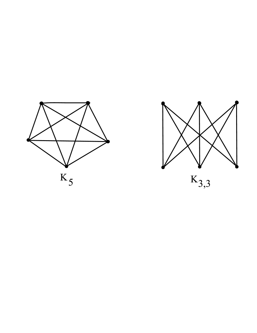
Figure 2. Graphs $K_{5}$ and $K_{3,3}$.

This follows by combining a theorem of A. Abrams [1] (stating that the spaces $F(K_{5},2)$ and $F(K_{3,3},2)$ are homotopy equivalent to closed orientable surfaces of genus 6 and 4, correspondingly) with Theorem 9 from [4] computing the invariant ${\rm\bf{TC}}$ for the surfaces. In these examples the equality(19) is again violated.

10. Configuration Spaces of Two Particles

In the present section we explicitly describe the topology of the configuration spaces $F(\Gamma,2)$ and $B(\Gamma,2)=F(\Gamma,2)/{\mathbf{Z}}_{2}$ where $\Gamma$ is a tree. The latter space is the quotient of $F(\Gamma,2)$ with respect to the involution interchanging the particles. The results of this section are used in the proof of Theorem 10.

Theorem 11.

Let $\Gamma$ be a tree having an essential vertex. Then the space $B(\Gamma,2)$ is homotopy equivalent to the wedge of

(25) $$\frac{1}{2}\sum_{v}(\eta(v)-1)(\eta(v)-2)$$

circles where $v$ runs over the vertices of $\Gamma$ and the symbol $\eta(v)$ denotes the number of edges incident to the vertex $v$.

Note that only essential vertices $v$ contribute nonzero summands to (25).

In the next theorem we identify the equivariant homotopy type of $F(\Gamma,2)$ with respect to the canonical involution interchanging the labels of the particles. Fix a univalent root vertex $u_{0}$ of $\Gamma$. Then any vertex $v\not=u_{0}$ has a well-defined single descending edge which is incident to it. It is the edge connecting $v$ with the root vertex: removing the descending edge makes $v$ and $u_{0}$ lying in different connected components. The other $\eta(v)-1$ edges incident to the vertex $v$ will be called ascending.

Theorem 12.

Let $\Gamma$ be a tree having an essential vertex. Then the space $F(\Gamma,2)$ is homotopy equivalent to the wedge of

(26) $$\sum_{v}(\eta(v)-1)(\eta(v)-2)-1$$

circles where $v$ runs over the vertices of $\Gamma$. Moreover, the ${\mathbf{Z}}_{2}$-equivariant homotopy type of $F(\Gamma,2)$ can be described as follows. Consider a 1-dimensional cell complex $Y_{\Gamma}$ having two vertices $A$ and $B$ and a number of 1-dimensional cells connecting $A$ to $B$, each labelled by an ordered pair of distinct ascending edges of $\Gamma$ incident to an essential vertex $v\in\Gamma$. In total there are $\sum_{v}(\eta(v)-1)(\eta(v)-2)$ such 1-cells. The complex $Y_{\Gamma}$ has an involution $T:Y_{\Gamma}\to Y_{\Gamma}$ which takes $A$ to $B$ and which takes the edge with the label $(e_{i},e_{j})$ to the edge with the label $(e_{j},e_{i})$. Then $F(\Gamma,2)$ and $Y_{\Gamma}$ are ${\mathbf{Z}}_{2}$-equivariantly homotopy equivalent.

Figure 3 illustrates the construction of the cell complex $Y_{\Gamma}$.

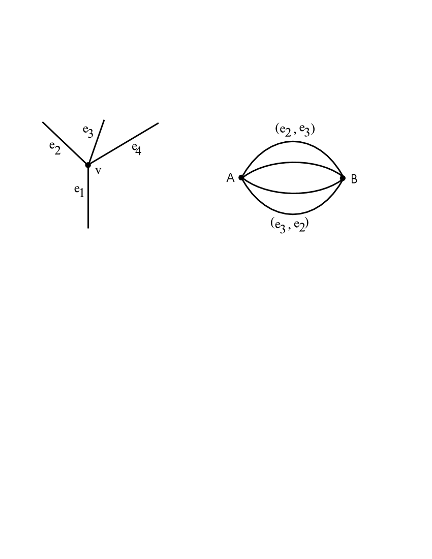
Figure 3. Descending edge $e_{1}$ and ascending edges $e_{2}$, $e_{3}$, $e_{4}$ incident to a vertex $v$ (left) and a part of the cell complex $Y_{\Gamma}$ (right).

The complex $Y_{\Gamma}$ can also be described as follows. Consider the standard unit sphere $S^{2}\subset\mathbf{R}^{3}$ given by the equation $x^{2}+y^{2}+z^{2}=1$. Let $P_{\phi}$ denotes the 2-dimensional plane spanned by the vectors $(0,0,1)$ and $(\cos\phi,\sin\phi,0)$. The intersection $P_{\phi}\cap S^{2}$ is a circle $S_{\phi}^{1}$ containing the North and the South poles $(0,0,\pm 1)$. Set $\phi_{i}=\frac{i\pi}{n}$ where $i=0,1,\dots,n-1$ and

$$n=1/2\cdot\sum_{v}\eta(v)-1)(\eta(v)-2),$$

the sum taken over the vertices of $\Gamma$. Then

(27) $$Y_{\Gamma}=\bigcup_{i=0}^{n-1}S^{1}_{\phi_{i}}.$$

The latter space is viewed with the standard antipodal involution.

11. Sketch of Proof of Theorem 10.

First we consider the special case when the tree $\Gamma$ has a single essential vertex, $m(\Gamma)=1$. Then, by a theorem of R. Ghrist [8], the configuration space $F(\Gamma,n)$ has homotopy type of a wedge of

(28) $$1+[(n-1)(\eta-2)-1]\cdot\frac{(n+\eta+2)!}{(\eta-1)!}$$

circles where $\eta=\eta(v)$ denotes the number of edges incident to the essential vertex. Using Theorem 4 we find that the topological complexity of the configuration space $F(\Gamma,n)$ equals either 2 or 3 depending on whether the number of circles in the wedge is 1 or $>1$. It is easy to see that (28) equals 1 if and only if $\eta=3$ and $n=2$. Since this possibility is excluded by our assumption we find that ${\rm\bf{TC}}(F(\Gamma,n))=3$ for $m(\Gamma)=1$.

The proof in the case $m(\Gamma)>1$ uses the following lemma:

Lemma 13.

Let $X$ be a topological space and let

(29) $$u_{1},\dots,u_{m},w_{1},\dots,w_{m}\in H^{1}(X)$$

be cohomology classes (where $H^{\ast}(X)=H^{\ast}(X;\mathbf{k})$ and ${\mathbf{k}}$ is a field) satisfying

(30) $$u_{i}w_{j}=0,\quad i,j=1,\dots,m,$$

and such that their cup-products $u_{1}\dots u_{m}$ and $w_{1}\dots w_{m}\in H^{m}(X)$ are linearly independent. Then

(31) $${\rm\bf{TC}}(X)\geq 2m+1.$$

Proof.

Consider the classes $\bar{u}_{i}=1\otimes u_{i}-u_{i}\otimes 1$ and $\bar{w}_{j}=1\otimes w_{j}-w_{j}\otimes 1$ lying in the tensor product $H^{\ast}(X)\otimes H^{\ast}(X)$. The classes $\bar{u}_{i}$ and $\bar{w}_{j}$ are zero-divisors. The product of all these classes in $H^{\ast}(X)\otimes H^{\ast}(X)$ equals

(32) $$\prod_{i=1}^{m}\bar{u}_{i}\cdot\prod_{j=1}^{m}\bar{w}_{j}\,=\,\pm\prod_{i=1}^{m}u_{i}\otimes\prod_{j=1}^{m}w_{j}\,\pm\,\prod_{j=1}^{m}w_{j}\otimes\prod_{i=1}^{m}u_{i}.$$

Since the classes $\prod_{i=1}^{m}u_{i}$ and $\prod_{j=1}^{m}w_{j}$ are linearly independent we may find two linear functionals $\phi,\psi:H^{m}(X)\to\mathbf{k}$ such that $\phi(\prod_{i=1}^{m}u_{i})\not=0$ and $\phi(\prod_{j=1}^{m}w_{j})=0$ while $\psi(\prod_{j=1}^{m}w_{j})\not=0$ and $\psi(\prod_{i=1}^{m}u_{i})=0$. Using (32) we see that applying $\phi\otimes\psi$ to the product (32) is nonzero which proves the non-triviality of the product (32). Hence we have a nontrivial product of $2m$ zero divisors. Applying Theorem 3 gives the desired result. ∎

Assume now that $\Gamma$ is a tree having $m(\Gamma)\geq 2$ essential vertices.

Let $v_{1},\dots,v_{m}$ be the essential vertices of $\Gamma$. The space $F(\Gamma,2)$ is homotopy equivalent to a wedge of circles (cf. Theorem 12). For any index $i=1,2,\dots,m$ we fix a nonzero cohomology class $\alpha_{i}\in H^{1}(F(\Gamma,2))$ with the only condition that it vanishes on all the circles in the wedge except the circles associated with the vertex $v_{i}$, see formula (26).

We define two continuous maps

$$\Phi_{i}:F(\Gamma,n)\to F(\Gamma,2),\quad\Psi_{i}:F(\Gamma,n)\to F(\Gamma,2),$$

where $i=1,2,\dots,m$ and

(39) $$\begin{array}[]{lll}\Phi_{i}(x_{1},\dots,x_{n})&=(x_{2i-1},x_{2i}),&\\ \\ \Psi_{i}(x_{1},\dots,x_{n})&=\left\{\begin{array}[]{ll}(x_{2i+1},x_{2i+2}),&\,\mbox{for}\,i=1,\dots,m-1,\\ \\ (x_{1},x_{2}),&\,\mbox{for}\,i=m.\end{array}\right.\end{array}$$

Finally we denote

(40) $$v_{i}=\Phi^{\ast}_{i}(\alpha_{i})\in H^{1}(F(\Gamma,n)),\quad w_{i}=\Psi_{i}^{\ast}(\alpha_{i})\in H^{1}(F(\Gamma,n)).$$

One checks that the conditions of Lemma 13 are satisfied for the constructed cohomology classes, i.e. the cup-products $u_{1}\cdots u_{m}$ and $w_{1}\cdots w_{m}$ are linearly independent and $u_{i}w_{j}=0$. Applying Lemma 13 completes the proof.

The full details will appear elsewhere.

12. Conclusion

The topological invariant ${\rm\bf{TC}}(X)$ imposes important restrictions on the structure of motion planning algorithms for the mechanical systems having $X$ as their configuration space. ${\rm\bf{TC}}(X)$ bounds from below the order of instability of deterministic motion planning algorithms. We prove in this paper that the number ${\rm\bf{TC}}(X)$ equals the minimal integer $k$ such that there exists a $k$-valued random motion planning algorithm in $X$.

The motion planning algorithm in the configuration space $F(\Gamma,n)$ of $n$ distinct points on a tree $\Gamma$ which is described in §8 has the minimal possible topological complexity, as Theorem 10 states. This algorithm may be used in practical control problems when several objects have to be moved along a tree $\Gamma$ avoiding collisions.

We observe that for a large number of particles $n$, the topological complexity of this algorithm depends only on the tree $\Gamma$ and does not depend on the number of the moving objects $n$.

This result could be compared with the earlier results of [7] which gives the topological complexity of the motion planning problem of many objects in the space $\mathbf{R}^{3}$ and on the plane $\mathbf{R}^{2}$. The topological complexity of the motion planning algorithms in these situations depends linearly on the number of particles; it equals $2n-2$ for $F(\mathbf{R}^{2},n)$ and is $2n-1$ for $F(\mathbf{R}^{3},n)$.

We obtain: for a large number of objects which must be simultaneously controlled avoiding collisions, a great simplification can be achieved by restricting the motion of the objects to a one-dimensional net.

This result may potentially have practical applications in some traffic control problems.

References

- [1] Abrams A. (2002) Configuration spaces of colored graphs. Geometriae Dedicata 92, 185 – 194
- [2] Dold A. (1972) Lectures on Algebraic Topology. Springer - Verlag.
- [3] Dubrovin B., Novikov S. P. and Fomenko A. T. (1984) Modern Geometry; Methods of the Homology Theory. Springer-Verlag.
- [4] Farber M. (2003) Topological Complexity of Motion Planning. Discrete and Computational Geometry 29, 211–221
- [5] Farber M. (2004) Instabilities of Robot Motion. Topology and its Applications (to appear). Available as preprint cs.RO/0205015.
- [6] Farber M, Tabachnikov S., Yuzvinsky S. (2003) Topological Robotics: Motion Planning in Projective Spaces. ”International Mathematical Research Notices” 34, 1853–1870
- [7] Farber M., Yuzvinsky S. (2004) Topological Robotics: Subspace Arrangements and Collision Free Motion Planning. To appear in AMS volume dedicated to S.P.Novikov’s 65th birthday. Available as preprint math.AT/0210115
- [8] Ghrist R. (2001) Configuration spaces and braid groups on graphs in robotics. Knots, braids, and mapping class groups – papers dedicated to Joan S. Birman, AMS/IP Stud. Adv. Math. 24, Amer. Math. Soc., Providence, 29 – 40
- [9] Ghrist R., Koditschek D. (2002) Safe cooperative robot dynamics on graphs. SIAM J. Control Optim. 40, 1556 – 1575
- [10] Halperin D., Sharir M. (1995) Arrangements and their applications in robotics: recent developments. The Algorithmic Foundations of Robotics. K. Goldberg, D. Halperin, J.C. Latombe and R. Wilson eds., Boston, MA, 495 - 511
- [11] Latombe J.-C. (1991) Robot Motion Planning. Kluwer Academic Publishers
- [12] Schwartz J. T., Sharir M. (1983) On the piano movers’ problem: II. General techniques for computing topological properties of real algebraic manifolds. Adv. Appl. Math., 4, 298–351
- [13] Schwarz A.S. (1966) The genus of a fiber space. Amer. Math. Sci. Transl. 55, 49- 140
- [14] Sharir M. (1997) Algorithmic motion planning. Handbook of Discrete and Computational Geometry. J.E. Goodman, J. O’Rourke eds. CRC Press, Boca Raton, FL, 733 - 754
- [15] Smale S. (1987) On the topology of algorithms, I. J. of Complexity, 3, 81-89.
- [16] Spanier E.(1966) Algebraic Topology.
Index
- essential vertex §7
- order of instability §1
- random motion planning algorithm Collision Free Motion Planning on Graphs, Definition 7
- random path §6