Application of the Wavelet Transform with a Piecewise Linear Basis to the Evaluation of the Hankel Transform

Abstract

A method for computing the Hankel transform is proposed whereby the letter is reduced to a sum by representing the integrand as a smooth function times a Bessel function. The smooth function is replaced by its wavelet decomposition with a basis such its scalar product with the Bessel function is calculated analytically. The result is represented as a series, with the coefficients strongly depending on the local behavior of the function being transformed. The application of the method is demonstrated by an example illustrated with plots.

The Hankel transform has found a wide variety of applications related to problems in mathematical physics that possess an axial symmetry (see [1]). The transforms of the zeroth ($n=0$) and first ($n=1$) kind,

$$\begin{array}[]{c}F_{n}(p)=\int\limits^{\infty}_{0}f(r)J_{n}(pr)rdr,\\ f(r)=\int\limits^{\infty}_{0}F_{n}(r)J_{n}(pr)pdp.\end{array}$$ (1)

are used most frequently. This is explained by the fact that, in Heaviside’s calculus, the Laplace operator as applied to a function is equivalent to multiplication in the Laplace transform space:

$$\left(\frac{d^{2}}{dr^{2}}+\frac{1}{r}\frac{d}{dr}\right)f(r)\longleftrightarrow-p^{2}F_{0}(p),\qquad\left(\frac{d^{2}}{dr^{2}}+\frac{1}{r}\frac{d}{dr}-\frac{1}{r^{2}}\right)f(r)\longleftrightarrow-p^{2}F_{1}(p),$$

In practice, however, this method encounters a number of difficulties. One of them is that integrals of type (1) cannot frequently be evaluated analytically in finite form. Moreover, on computer, the function being transformed is specified as a set of numbers. Thus, an important task is to develop numerical methods for computing the Hankel transform with allowance made for the fact that $J_{n}(pr)$ is a rapidly oscillating function for large values of $p$ (or $r$). Two approaches to the solution of this problem are available in the literature. The first is the fast Hankel transform, which was originally proposed in [2] and has been improved up to the present (e.g., see Appendix B in [3] and the references therein). This approach involves making a substitution and scaling, which reduce the problem to logarithmic coordinates and the fast Fourier transform. This method applies to tabulated functions, but it involves conventional errors arising when a nonperiodic function is replaced by its periodic extension. Additionally, the method is sensitive to the smoothness of functions in the space of logarithmic coordinates. An efficient algorithm (also based on the fast Fourier transform) was proposed for commuting the discrete Hankel (Fourier–Bessel) transform in [4]. It was noted in [4] that the algorithm is applicable in the case of an integral transform approximated by a sum. Another method (see [5]) involves the representation of the integrand as the product of a smooth function approximated by a set of polynomials and an oscillating function such that the integral of its product with the polynomial can be computed analytically. The accuracy of this approach is limited primarily by the accuracy of the polynomial approximation of the function to be transformed.

The basic idea behind our method is similar to that in [5]. However, instead of a single approximation of the smooth factor, we apply its multiscale decomposition with respect to a function basis that takes into account the local properties of the function being transformed. Moreover, the scalar product of basis functions must be calculated analytically.

These conditions are satisfied by some spline wavelet decompositions, which have been intensively studied in recent years (e.g., see [6–8]). Let $g(r)$ be a function in $L^{2}(R)$. Then it can be represented as a series

$$g(r)=\sum_{j\in Z}\sum_{k\in Z}d_{jk}\psi_{jk}(r),$$ (2)

where $\psi_{jk}(r)=2^{j/2}\psi{2^{j}r-k}$ are basis functions with step $k$ and scale $j$ that satisfy the conditions of spatial localization and self-similarity under scale changes. The latter means that all $\psi_{jk}$ are formed by contracting and translating a single function $\psi$.

Since the direct and inverse Hankel transforms (1) are symmetric, we restrict our consideration to the direct transform and set $g(r)=f(r)r$ for simplicity. Substituting (2) into the integral gives

$$F_{n}(p)=\sum_{j\in Z}\sum_{k\in Z}d_{jk}\int\limits^{\infty}_{0}\psi_{jk}(r)J_{n}{pr}dr.$$ (3)

Consider piecewise linear wavelets. Suppose that the basis wavelet is the piecewise linear function

$$\psi(r)=\sum_{m}\frac{r-mh}{h}b_{m+1}-\frac{r-(m+1)h}{-h}b_{m},$$

where $b_{m}$ are the values at the junction points and $h$ is the minimum step.

The limits of summation are determined by the type of the wavelet chosen. In particular, as a basis, one can use the Battle–Lemarie $\psi^{B,2}$ and Strömberg $\psi^{St,2}$ orthogonal wavelets [6], which are an infinite set of linear segments, or one can apply semiorthogonal or biorthogonal bases with a compact support consisting of $M$ segments. Examples of the latter are B-spline semiorthogonal wavelets [8], biorthogonal wavelets obtained by applying the lifting scheme [9], and BlaC-wavelets (Blending of Linear and Constant) [10], which combine a piecewise linear and a piecewise constant function. Note that the Battle– Lemarie and Strömberg bases rapidly decay at infinity, even though they have no compact support. Thus, they can be truncated to $M$ segments in practical computations. Applying the integration formulas of [11], we find that the Hankel transform is equivalent to a sum:

$$\begin{array}[]{l}F_{0}(p)=\frac{1}{p}\sum\limits_{j\in Z}{\sum\limits_{k\in Z}{2^{j/2}}}d_{jk}\sum\limits_{m}{\left({(b_{k+1}-b_{k})\left[{(k+m+1)J_{1}(2^{-j}(k+m+1)hp)-}\right.}\right.}\\ \left.{-(k+m)J_{1}(2^{-j}(k+m)ph)}\right]+\left[{(k+m+1)b_{k}-(k+m)b_{k+1}}\right]\times\\ \left\{{(k+m+1)J_{0}(2^{-j}(k+m+1)hp)}\right.-(k+m)J_{0}(2^{-j}(k+m)ph)+\\ \left.{\left.{\frac{\pi}{2}\left[{(k+m+1)D(2^{-j}(k+m+1)hp)-(k+m)D(2^{-j}(k+m)ph)}\right]}\right\}}\right)\\ \end{array}$$ (4)

$$\begin{array}[]{l}F_{1}(p)=\frac{1}{p}\sum\limits_{j\in Z}{\sum\limits_{k\in Z}{2^{j/2}}}d_{jk}\sum\limits_{m}{\left({\frac{{\pi(b_{k+1}-b_{k})}}{2}\left[{(k+m+1)D(2^{-j}(k+m+1)hp)-}\right.}\right.}\\ \left.{-(k+m)D(2^{-j}(k+m)ph)}\right]+\left[{(k+m+1)b_{k}-(k+m)b_{k+1}}\right]\times\\ \left.{\left\{{(k+m+1)J_{0}(2^{-j}(k+m)hp)}\right.\left.{-(k+m)J_{0}(2^{-j}(k+m+1)ph)}\right\}}\right)\\ \end{array}$$ (5)

where $D(x)=H_{0}(x)J_{1}(x)-H_{1}(x)J_{0}(x)$ and $H_{0,1}$ are Struve functions [11].

Thus, if the function being transformed (which is completely characterized by its coefficients [6–8]) has a finite-form definite integral of its product with a linear function, then series (4) and (5) are an exact representation of the Hankel transform as a sum. Note that for sufficiently smooth functions strongly varying only in small ranges of their arguments, most of the $d$-coefficients in (4) and (5) are small for high levels of resolution $j$. This makes it possible to derive an approximate numerical Hankel transform from multiscale analysis, in which case compactly supported bases have a significant advantage, because they avoid additional errors associated with the finite length of the function ranges used in numerical computations. Suppose that the function to be transformed is specified as a set of $N$ points, which are interpreted as its projection on an interval onto the space of scaling functions of resolution $J\leq\log_{2}N$. Then (2) is replaced by the series

$$g(r)=\sum_{j=0}^{J}\sum{k}d_{jk}\psi_{jk}(r)+\sum_{k}s_{Jk}\varphi{Jk}(r),$$

where $\varphi_{0k}$ is a scaling function of a coarser resolution. In the computations, one can use only those of the coefficients $d_{jk}$ that are greater than a prescribed small number $\varepsilon$. The accuracy of the approximation of $g$ by a truncated function $g_{\varepsilon}$ [7] is defined as $\Delta=\left(\|g-g_{\varepsilon}\|\right)^{1/2}=\left(\left\|\sum d_{jk}^{*}\psi_{jk}\right\|^{2}\right)^{2}$ . Taking into account the orthogonality of the basis wavelets, we obtain $\Delta\leq\varepsilon n_{0}^{1/2}$, where $n_{0}$ is the number of discarded coefficients $d_{jk}^{*}\leq\varepsilon$. The resulting set contains wide bands of zeros in the domain where the function is smooth and an increased number of coefficients in the domain where it undergoes abrupt changes. Since the basis wavelet functions are narrowly localized, this implies a high degree of adaptivity in choosing an interpolation grid. Series (4) and (5) preserve their form when the limits in $j$ and $k$ are changed or terms are added that correspond to scalar products with scaling functions representable in a similar form.

Thus, the integral transforms have been reduced to sums. For small arguments of the Bessel function, they can be computed by conventional codes and, for large arguments, by applying algorithms developed, for example, in [4].

Numerical computations in the case where $g(r)$ is defined analytically are interesting on their own. For this purpose, we can use an inverse version of the lifting scheme [9] for piecewise linear basis functions. Let a function be defined on the interval $[0,\quad 1]$ (this can always be achieved by suitable scaling). This interval is bisected (the crudest approximation) and the lifting scheme is applied to a set of three function values (at the endpoints and the middle of the interval) to obtain the first iterates

$$\gamma_{00}=g\left(\frac{1}{2}\right)-\frac{1}{2}\sum_{k=0}^{1}g(k),\qquad\lambda_{k}=g(k)+\frac{1}{4}\gamma_{00},$$

$$V_{0}(x)=\sum_{k=0}^{1}\lambda_{k}\varphi_{0k}(x),\qquad W_{0}(x)=\gamma_{00}\psi_{00}(x),\qquad g(x)\approx V_{0}(x)+W_{0}(x).$$

If the detailed coefficient $\gamma_{00}$ is not small, then the set is supplemented with the values of $g(r)$ calculated at the middle points of each half-interval, and the next iterates are computed as follows. Calculate the detailed coefficient of coarser level $J$:

$$\gamma_{jk}=g\left[2^{-(J+k)}(2k+1)\right]-V_{0}\left[2^{-(J+k)}(2k+1)\right]-W_{J-1}\left[2^{-(J+k)}(2k+1)\right].$$

By using this relation, the detailed coefficients of the preceding levels and the approximation coefficients are updated to give

$$\gamma_{jk}=\gamma_{jk}-W_{J}\left(2^{-(J+1)}(2k+1)\right),\quad,j=\overline{0,J-1},$$

$$\gamma_{jk}=\gamma_{jk}-W_{J}\left(2^{-(J+1)}(2k+1)\right).$$

Here $W_{J}$ means all corresponding levels of the wavelet transform of difference between $g(r)$ and the transform of level $J-1$.

The current representation of the function being decomposed is formed by

$$\sum\limits_{k=0}^{1}{\lambda_{k}\varphi_{0k}(x),\quad W_{j}(x)=}\sum\limits_{j=0}^{J}{\sum\limits_{k=0}^{2^{j}-1}{\gamma_{jk}\psi_{jk}(x),\quad g(x)\approx V_{0}(x)+\sum\limits_{j=0}^{J}{W_{j}(x);}}}$$

Here, the scaling function and the basis wavelet are given by

$$\varphi_{0k}(x)=\Lambda(x-k),\quad\phi(x)=\Lambda(2x-1)-\frac{1}{4}\Lambda(x)-\frac{1}{4}\Lambda(x-1),$$

where $\Lambda(x)=\max\{0,1-|x|\}$.

As an example, we consider a function that has an exact first-kind Hankel transform:

$$f(r)=re^{-ar^{2}},\quad F_{1}(p)=\frac{p}{(2a^{2})^{2}}\exp\left(-\frac{p^{2}}{4a^{2}}\right).$$

Let $a=0.4$. Then the basic nonzero part of the function is concentrated on the interval $[0,\quad 8]$. By making the substitution $r^{*}=r/8$, this interval is transformed into a unit interval, and the above procedures for wavelet decomposition with updating and the Hankel transform (5) are applied to $g(r^{*})=f(r^{*})r^{*}$.

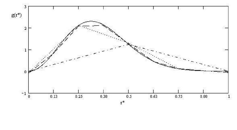
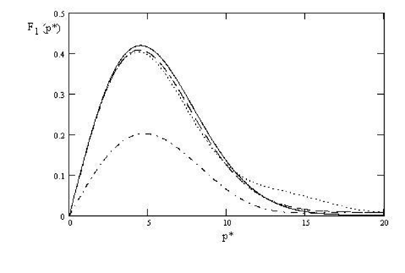
Figure 1:

Figure 2:

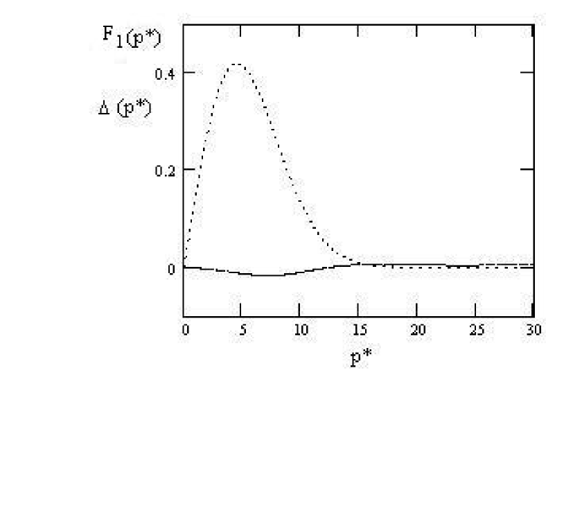
Figure 3:

Figure 1 shows the plot of $g(r^{*})$ (solid curve) and its wavelet representations at the zeroth (dot-and-dash), first (dotted), and second (dashed) levels. The corresponding curves in Fig. 2 plot the exact and approximate Hankel transforms in these cases. It can be seen that even this small number of levels provides an adequate pattern (except for the zeroth approximation, which gives a rather crude representation of the original function because of using the function value at the middle point of the interval). The next level provides a good approximation for most of the curve, except for large values of $p^{*}$. This domain is corrected by the second approximation. Figure 3 shows the absolute error for this level, $\Delta(p^{*})$, which is equal to the difference between the approximate (dotted) and exact (solid) solutions against the background of the exact transform. It can be seen that the absolute error is fairly small in the entire domain shown in the figure and does not increase sharply with $p^{*}$. The computed solution is as accurate as that obtained by linear approximation at the same nodes. However, our method provides rough estimation over the entire domain of the function, with subsequent refinement over intervals of interest. An improved accuracy in this approach can be achieved not only by increasing the number of decomposition levels taken into account but also by using a basis with unequally spaced nodes adapted to the behavior of the function to be transformed.

References

- [1] C. J. Tranter, Integral Transforms in Mathematical Physics (Methuen, London, 1951).
- [2] A. E. Siegman, Optics. Lett., No. 1, 13 (1977).
- [3] A. J. S. Hamilton, Mon. Not. R. Astron. Soc. 312, 257 (2000).
- [4] Ya. M. Zhileikin and A. B. Kukarkin, Zh. Vychisl. Mat. Mat. Fiz. 35, 1128 (1995).
- [5] R. Barakat and E. Parshall, Appl. Math. Lett., No. 5, 21 (1996).
- [6] S. B. Stechkin and I. Ya. Novikov, Usp Mat. Nauk 53, 53 (1998).
- [7] I. N. Dremin, O. V. Ivanov, and V. A. Nechitailo, Usp. Fiz. Nauk 171, 465 (2001).
- [8] C. K. Chui, An Introduction to Wavelets (Academic, Boston 1992; Mir, Moscow, 2001).
- [9] W. Sweldens, in ”Proceedings of Wavelet Applications in Signal and Image Processing III” SPIE Proceedings Series 2569 (SPIE, Bellingham, 1995), p. 68.
- [10] G.-P. Bonneau, S. Hahmann, and G. M. Nielson, in ”Proceedings of VIS’96,” (ACM, New York, 1996), p. 43.
- [11] Handbook of Mathematical Functions, with Formulas, Graphs, and Mathematical Tables, Ed. by M. Abramowitz and I. A. Stegun (Dover, New York, 1972).