Abstract

Suppose that $N$ is a geometrically finite orientable hyperbolic $3$-manifold. Let ${\mathcal{P}}(N,\underline{\alpha})$ be the space of all geometrically finite hyperbolic structures on $N$ whose convex core is bent along a set $\underline{\alpha}$ of simple closed curves. We prove that the map which associates to each structure in ${\mathcal{P}}(N,\underline{\alpha})$ the lengths of the curves in the bending locus $\underline{\alpha}$ is one-to-one. If $\underline{\alpha}$ is maximal, the traces of the curves in $\underline{\alpha}$ are local parameters for the representation space ${\mathcal{R}}(N)$.

Key words: convex structure, cone manifold, bending lamination

1 Introduction

This paper is about the parameterization of convex structures on hyperbolic $3$-manifolds. We show that the space of structures whose bending locus is a fixed set of closed curves $\underline{\alpha}=\{{\alpha}_{1},\ldots,{\alpha}_{n}\}$ is parameterized by the hyperbolic lengths $\{l_{{\alpha}_{1}},\ldots,l_{{\alpha}_{n}}\}$ and moreover, that when $\underline{\alpha}$ is maximal, the complex lengths (or traces) of the same set of curves are local holomorphic parameters for the ambient deformation space.

Suppose that $N(G)={\mathbb{H}}^{3}/G$ is a hyperbolic $3$-manifold such that $G$ is geometrically finite with non-empty regular set and such that its convex core $V=V(G)$ has finite but non-zero volume. The boundary of $V$ is always a pleated surface, with bending locus a geodesic lamination $pl(G)$. Assume that $V(G)$ has no rank-$2$ cusps. All our main results hold without this assumption, but writing down the proofs in full generality does not seem to warrant all the additional comments and notation entailed. If $V$ has rank-$1$ cusps, compactify $V$ by removing a horoball neighborhood of each cusp. The interior of the resulting manifold $\bar{N}(G)$ is homeomorphic to ${\mathbb{H}}^{3}/G$. The boundary of $\bar{N}(G)$ consists of closed surfaces obtained from ${\partial}V$ by removing horospherical neighborhoods of matched pairs of punctures and replacing them with annuli, see Figure 1. Denote by $\underline{\alpha}_{P}(G)$ the collection of core curves of these annuli.

Now let $\bar{N}$ be a compact orientable $3$-manifold whose interior $N$ admits a complete hyperbolic structure. Assume that the boundary ${\partial}\bar{N}$ is non-empty and that it contains no tori. Let $\underline{{\alpha}}=\{{\alpha}_{1},\ldots,{\alpha}_{m}\}$ be a collection of disjoint, homotopically distinct simple closed curves on ${\partial}\bar{N}$. In this paper we investigate hyperbolic $3$-manifolds ${\mathbb{H}}^{3}/G$ such that $\bar{N}(G)$ is homeomorphic to $\bar{N}$ and such that the bending locus of ${\partial}V$, together with the set $\underline{\alpha}_{P}(G)$ of core curves of the annuli described above, consists exactly of the curves in $\underline{\alpha}$. Denote by $\mathcal{P}^{+}(N,\underline{\alpha})$ the space of all such structures, topologized as a subset of the representation space $\mathcal{R}(N)=Hom(\pi_{1}(N),SL(2,{\mathbb{C}}))/SL(2,{\mathbb{C}})$, where $Hom(\pi_{1}(N),SL(2,{\mathbb{C}}))$ is the space of homomorphisms from $\pi_{1}(N)$ to $SL(2,{\mathbb{C}})$ and $SL(2,{\mathbb{C}})$ acts by conjugation. More generally, define the pleating variety ${\mathcal{P}}(N,\underline{\alpha})$ to be the space of structures for which the bending locus of ${\partial}V$ and $\underline{\alpha}_{P}(G)$ are contained in, but not necessarily equal to, $\underline{\alpha}$. We refer to a structure in ${\mathcal{P}}(N,\underline{\alpha})$ as a convex structure on $(\bar{N},\underline{\alpha})$. We emphasize that structures in ${\mathcal{P}}(N,\underline{\alpha})$ must have convex cores with finite non-zero volume, thus excluding the possibility that the group $G$ is Fuchsian.

For ${\alpha}_{i}\in\underline{\alpha}$, let $\theta_{i}$ be the exterior bending angle along ${\alpha}_{i}$, measured so that $\theta_{i}=0$ when ${\alpha}_{i}$ is contained in a totally geodesic part of ${\partial}V$, and set $\theta_{i}=\pi$ when ${\alpha}_{i}\in\underline{\alpha}_{P}(G)$. Then $\mathcal{P}^{+}(N,\underline{\alpha})$ is the subset of ${\mathcal{P}}(N,\underline{\alpha})$ on which $\theta_{i}>0$ for all $i$.

In [5], Bonahon and Otal gave necessary and sufficient conditions for the existence of a convex structure with a given set of bending angles. They show:

Theorem 1.1 (Angle parameterization)

Let $\Theta:{\mathcal{P}}^{+}(N,\underline{\alpha})\rightarrow{\mathbb{R}}^{n}$ be the map which associates to each structure $\sigma$ the bending angles $(\theta_{1}(\sigma),\ldots,\theta_{n}({\sigma}))$ of the curves in the bending locus $\underline{\alpha}=\{{\alpha}_{1},\ldots,{\alpha}_{n}\}$. Then $\Theta$ is a diffeomorphism onto a convex subset of $(0,\pi]^{n}$.

Moreover, the image is entirely specified by the topology of $\bar{N}$ and the curve system $\underline{\alpha}$. Reformulating their conditions topologically, we show in Theorem 2.4 that $\mathcal{P}^{+}(N,\underline{\alpha})$ is non-empty exactly when the curves $\underline{\alpha}$ form a doubly incompressible system on ${\partial}\bar{N}$, see Section 2.3. Thus their result shows that, provided these topological conditions are satisfied, ${\mathcal{P}}^{+}(N,\underline{\alpha})$ is a submanifold of $\mathcal{R}(N)$ of real dimension equal to the number of curves in $\underline{\alpha}$, and that the bending angles uniquely determine the hyperbolic structure on $N$.

In this paper we prove an analogous parameterization theorem for ${\mathcal{P}}(N,\underline{\alpha})$ in which we replace the angles along the bending lines by their lengths.

Theorem A (Length parameterization)

Let $L:{\mathcal{P}}(N,\underline{\alpha})\rightarrow{\mathbb{R}}^{n}$ be the map which associates to each structure $\sigma$ the hyperbolic lengths $(l_{{\alpha}_{1}}(\sigma),\ldots,l_{{\alpha}_{n}}({\sigma}))$ of the curves in the bending locus $\underline{\alpha}=\{{\alpha}_{1},\ldots,{\alpha}_{n}\}$. Then $L$ is an injective local diffeomorphism.

This follows from our stronger result that any combination of lengths and angles also works:

Theorem B (Mixed parameterization)

For any ordering of the curves $\underline{\alpha}$ and for any $k$, the map $\sigma\mapsto(l_{\alpha_{1}}({\sigma}),\ldots,l_{\alpha_{k}}({\sigma}),\theta_{\alpha_{k+1}}({\sigma}),\ldots,\theta_{\alpha_{n}}({\sigma}))$ is an injective local diffeomorphism on ${\mathcal{P}}(N,\underline{\alpha})$.

Remark With some further work, one can show that $L$ is actually a diffeomorphism onto its image. We hope to explore this, together with some applications of the parameterization, elsewhere.

It is known that in the neighborhood of a geometrically finite representation, ${\mathcal{R}}(N)$ is a smooth complex variety of dimension equal to the number of curves $d$ in a maximal curve system on ${\partial}\bar{N}$ (see Theorem 3.2). Theorem A follows from the following result on local parameterization:

Theorem C (Local parameterization)

Let $\sigma_{0}\in{\mathcal{P}}(N,\underline{\alpha})$, where $\underline{\alpha}=\{{\alpha}_{1},\ldots,{\alpha}_{d}\}$ is a maximal curve system on ${\partial}\bar{N}$. Then the map ${\mathcal{L}}:{\mathcal{R}}(N)\rightarrow{\mathbb{C}}^{d}$ which associates to a structure $\sigma\in\mathcal{R}(N)$ the complex lengths $(\lambda_{{\alpha}_{1}}(\sigma),\ldots,\lambda_{{\alpha}_{d}}(\sigma))$ of the curves ${\alpha}_{1},\ldots,{\alpha}_{d}$ is a local diffeomorphism in a neighborhood of $\sigma_{0}$.

To be precise, if ${\sigma}_{0}({\alpha}_{i})$ is parabolic, then $\lambda_{{\alpha}_{i}}({\sigma})$ must be replaced with $\mathop{\rm Tr}{\sigma}({\alpha}_{i})$ in the definition of ${\mathcal{L}}$. This point, together with a precise definition of the complex length $\lambda_{{\alpha}_{i}}(\sigma)$, is discussed in detail in Section 3.1. It is not hard to show that when restricted to $\mathcal{P}(N,\underline{\alpha})$, the map $\mathcal{L}:{\mathcal{R}}(N)\rightarrow{\mathbb{C}}^{d}$ is real-valued and coincides with $L$. We remark that the map ${\mathcal{L}}$ is not globally non-singular; in fact we showed in [32] that if $G$ is quasifuchsian, then $\mbox{d}{\mathcal{L}}$ is singular at Fuchsian groups on the boundary of $\mathcal{P}(N,\underline{\alpha})$.

The origin of these results was [23], which proved the above theorems in the very special case of quasifuchsian once-punctured tori, using much more elementary techniques. In [10] we carried out direct computations which proved Theorem A for some very special curve systems on the twice punctured torus. The results should have various applications. For example, combining Theorem A with [32], when the holonomy of $N$ is quasifuchsian, one should be able to exactly locate $\mathcal{P}(N,\underline{\alpha})$ in $\mathcal{R}(N)$.

As in [5], our main tool is the local deformation theory of cone manifolds developed by Hodgson and Kerckhoff in [17]. Let $M$ be the $3$-manifold obtained by first doubling $\bar{N}$ across its boundary and then removing the curves $\underline{\alpha}$. It is easy to see that a convex structure on $\bar{N}$ gives rise to a cone structure on $M$ with singular locus $\underline{\alpha}$. This means that everywhere in $M$ there are local charts to ${\mathbb{H}}^{3}$, except near a singular axis ${\alpha}$, where there is a cone-like singularity with angle $2(\pi-\theta_{{\alpha}})$. Under the developing map, the holonomy of the meridian $m_{{\alpha}}$ around ${\alpha}$ is an elliptic isometry with rotation angle $2(\pi-\theta_{{\alpha}})$. The local parameterization theorem of Hodgson and Kerckhoff (see our Theorem 3.3) states that in a neighborhood of a cone structure with singular axes $\underline{\alpha}=\{{\alpha}_{1},\ldots,{\alpha}_{d}\}$ and cone angles at most $2\pi$, the representation space ${\mathcal{R}}(M)$ is locally a smooth complex variety of dimension $d$, parameterized by the complex lengths $\mu_{{\alpha}}$ of the meridians. Notice that for a cone structure, $\mu_{{\alpha}}$ is $\sqrt{-1}$ times the cone angle. Moreover, the condition that the $\mu_{{\alpha}}$ are purely imaginary characterizes the cone structures. This leads to a local version of the Bonahon-Otal parameterization of convex structures in terms of bending angles.

To prove Theorem C, we use the full force of the holomorphic parameterization of ${\mathcal{R}}(M)$ in terms of the $\mu_{{\alpha}}$. Under the hypothesis that $\underline{\alpha}=\{{\alpha}_{1},\ldots,{\alpha}_{d}\}$ is maximal, the spaces ${\mathcal{R}}(M)$ and ${\mathcal{R}}(N)$ have the same complex dimension $d$. Moreover, we have the natural restriction map $r:{\mathcal{R}}(M)\rightarrow{\mathcal{R}}(N)$. Consider the pull-back $F=\mathcal{L}\circ r:{\mathcal{R}}(M)\rightarrow{\mathbb{C}}^{d}$ of the complex length function to ${\mathcal{R}}(M)$. Let $\rho_{0}\in{\mathcal{R}}(M)$ be the holonomy representation of the cone structure obtained by doubling the convex structure $\sigma_{0}\in{\mathcal{P}}(N,\underline{\alpha})$. Theorem C will follow if we show that $F$ is a local diffeomorphism near $\rho_{0}$. The key idea is that $F$ is a ‘real map’, that is, having identified the cone structures in ${\mathcal{R}}(M)$ with ${\mathbb{R}}^{d}$ (strictly speaking with $(i{\mathbb{R}})^{d}$), it has the properties:

$$F({\mathbb{R}}^{d}) \subset {\mathbb{R}}^{d}$$ (1)

$$F^{-1}({\mathbb{R}}^{d}) \subset {\mathbb{R}}^{d}.$$ (2)

Using the fact that $F$ is holomorphic, we show in Proposition 6.4 that this is sufficient to guarantee that $F$ has no branch points and is thus a local diffeomorphism.

The first inclusion (1) is relatively easy; the local parameterization by cone angles allows us to show that, near the double of a convex structure, the holonomy of any curve fixed by the doubling map has real trace (Corollary 5.4). Now consider the inclusion (2). We factor $F^{-1}({\mathbb{R}}^{d})$ as $r^{-1}(\mathcal{L}^{-1}({\mathbb{R}}^{d}))$ and consider each of the preimages separately. In Section 4 we use geometrical methods to prove the local pleating theorem, Theorem 4.2, which states that near $\sigma_{0}$, convex structures are characterized by the condition that the complex lengths of the curves in the bending locus are real. (Actually we have to introduce a slightly more general notion of a piecewise geodesic structure, in which we allow that some of the bending angles may be negative, corresponding to some cone angles greater than $2\pi$.) Thus ${\mathcal{L}}^{-1}({\mathbb{R}}^{d})$ is locally contained in ${\mathcal{P}}(N,\underline{\alpha})$. The second main step in our proof, Theorem 5.1, uses the duality between the meridians and the curves in the bending locus to show that $r$ is a local holomorphic bijection between ${\mathcal{R}}(M)$ and ${\mathcal{R}}(N)$. To finish the proof of (2), note that every convex structure is the restriction of some cone structure, namely, its double. However, since by Theorem 5.1 the map $r$ is one-to-one, the inverse image $r^{-1}(\sigma)$ of a convex structure $\sigma$ near $\sigma_{0}$ can only be its double, and thus a cone structure as required.

The plan of the rest of the paper is as follows. Sections 2 and 3 supply definitions and background. In Section 2.3 we prove the topological characterization Theorem 2.4 of which curve systems can occur, giving some extra details in the Appendix. In order to simplify subsequent arguments, we also show (Proposition 2.8) that the holonomy representation of a cone structure coming from doubling a convex structure can always be lifted to a representation into $SL(2,{\mathbb{C}})$. Section 3 contains a brief review of the relevant deformation theory, in particular expanding on the precise details of the Hodgson-Kerckhoff parameterization near cusps.

The deduction of the global parameterization theorem, Theorem A, from the local version Theorem C is carried out in Section 6. The main idea is to observe that the Jacobian of the map $\mathcal{L}$ restricted to $\mathcal{P}(N,\underline{\alpha})$, is the Hessian of the volume. We deduce that it is positive definite and symmetric, from which follow both the injectivity in Theorems A and B and some additional information on volumes of convex cores.

Acknowledgments We would like to thank Steve Kerckhoff and Max Forester for their insightful comments and help, always dispensed with much generosity. We would also like to thank Darryl McCullough for detailed suggestions about the Appendix. The second author is grateful for the support of her EPSRC Senior Research Fellowship.

2 Convex structures and their doubles

2.1 The bending locus

The background material in this section is explained in detail in  [27] and  [29]. We give a brief summary of the notions we will need. Let $G$ be a geometrically finite Kleinian group of the second kind, so that its regular set $\Omega(G)$ is non-empty. Let $\mathcal{H}(G)$ be the hyperbolic convex hull of the limit set $\Lambda(G)$ in ${\mathbb{H}}^{3}$, and assume that $\Lambda(G)$ is not contained in a circle, or equivalently, that the interior of $\mathcal{H}(G)$ is non-empty. The convex core of $N(G)={\mathbb{H}}^{3}/G$ is the $3$-manifold with boundary $V=V(G)=\mathcal{H}(G)/G$. Alternatively, $V(G)$ is the smallest closed convex subset of $N(G)$ which contains all closed geodesics. As stated in the introduction, we assume that $V(G)$ contains no rank-$2$ cusps.

As a consequence of the Ahlfors finiteness theorem, the boundary ${\partial}V$ of $V$ consists of a finite union of surfaces, each of negative Euler characteristic and each with possibly a finite number of punctures. Geometrically, each component $S_{j}$ of ${\partial}V$ is a pleated surface whose bending locus is a geodesic lamination $pl(S_{j})$ on $S_{j}$, see for example [11].

In this paper we confine our attention to the case of rational bending loci, in which the bending lamination of each $S_{j}$ is a set of disjoint, homotopically distinct simple closed geodesics $\{{\alpha}_{j_{1}},\ldots,{\alpha}_{j_{n_{j}}}\}$. We will use only the union of these curves, renumbering them as $\{{\alpha}_{1},\ldots,{\alpha}_{m}\}$, so that $m=\sum n_{j}$. Let $\theta_{i}\in(0,\pi)$ denote the exterior bending angle on ${\alpha}_{i}$ measured so that $\theta_{i}\rightarrow 0$ as the outwardly oriented facets of ${\partial}V$ meeting along ${\alpha}_{i}$ become coplanar.

It is convenient to modify the set $\{{\alpha}_{1},\ldots,{\alpha}_{m}\}$ so as to include the rank-$1$ cusps of ${\partial}V$ as follows. Let $\bar{N}(G)$ be the compact $3$-manifold with boundary obtained from $V$ by removing a horoball neighborhood of each cusp. Since $G$ is geometrically finite, $\bar{N}(G)$ is compact; the notation has been chosen to indicate that its interior is homeomorphic to $N(G)$. More precisely, choose $\epsilon>0$ sufficiently smaller than the Margulis constant, so that the $\epsilon$-thin part $V_{(0,\epsilon]}$ (consisting of points in $V$ at which the injectivity radius is at most $\epsilon$) consists only of finitely many disjoint rank-$1$ cusps. Define $\bar{N}(G)$ to be the underlying manifold of the $\epsilon$-thick part $V_{[\epsilon,\infty)}$. Note that for any $\epsilon^{\prime}<\epsilon$, there is a strong deformation retract of $V_{[\epsilon^{\prime},\infty)}$ onto $V_{[\epsilon,\infty)}$, and hence as a topological manifold, $\bar{N}(G)$ is well-defined, independent of the choice of $\epsilon$.

The intersection $V_{\epsilon}=V_{[\epsilon,\infty)}\cap V_{(0,\epsilon]}$ consists of the incompressible annuli which come from the rank-$1$ cusps, see [29] for more details. The boundary ${\partial}\bar{N}(G)$ consists of the closed surfaces obtained from ${\partial}V$ by removing horospherical neighborhoods of pairs of punctures and replacing them with the annuli in $V_{\epsilon}$, as shown in Figure 1. Conversely, we see that ${\partial}V$ can be obtained from ${\partial}\bar{N}(G)$ by pinching the core curves of $V_{\epsilon}$.

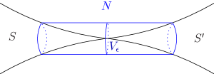
Figure 1: Replacing a pair of punctures with an annulus.

Denote the core curves in $V_{\epsilon}$ by $\underline{\alpha}_{P}(G)=\{{\alpha}_{m+1},\ldots,{\alpha}_{n}\}$.

We define the bending locus of $G$ to be the set $pl(G)=\{{\alpha}_{1},\ldots,{\alpha}_{n}\}$. We assign the bending angle $\pi$ to each curve in $\underline{\alpha}_{P}(G)$, corresponding to the fact that two facets of ${\partial}V$ which meet in a rank-$1$ cusp as in Figure 1, lift to planes in ${\mathbb{H}}^{3}$ which are tangent at infinity, in which case the angle between their outward normals is $\pi$.

2.2 Definition of a convex structure

In order to study variations of the structure defined in the last section, we now make a more general topological discussion. Let $\bar{N}$ be a compact orientable $3$-manifold whose interior $N$ admits a geometrically finite hyperbolic structure. Assume that ${\partial}\bar{N}$ is non-empty and contains no tori. A curve system on ${\partial}\bar{N}$ is a collection of disjoint simple closed curves $\underline{{\alpha}}=\{{\alpha}_{1},\ldots,{\alpha}_{n}\}$ on ${\partial}\bar{N}$, no two of which are homotopic in ${\partial}\bar{N}$. In light of the previous section, we designate a subset $\underline{\alpha}_{P}$ of $\underline{\alpha}$ as the parabolic locus. The previous section describes a generic convex structure on $(\bar{N},\underline{\alpha})$. We wish however, to be slightly broader, by allowing the bending angles on some of the curves in $\underline{\alpha}$ to vanish. It is convenient to begin with the following slightly more general definition. Note that both $\bar{N}$ and $\bar{N}-\underline{\alpha}_{P}$ are homotopically equivalent to $N$.

Definition 2.1

A piecewise geodesic structure on $(\bar{N},\underline{{\alpha}})$ with parabolic locus $\underline{\alpha}_{P}$ consists of a pair $(G,\phi)$, where $G$ is a geometrically finite Kleinian group whose convex core has non-zero volume and where $\phi:\bar{N}-\underline{\alpha}_{P}\hookrightarrow N(G)$ is an embedding such that the following properties are satisfied:
(i) $\phi_{*}:\pi_{1}(N)\rightarrow\pi_{1}(N(G))$ is an isomorphism;
(ii) $\phi_{*}(\gamma)$ generates a maximal parabolic subgroup for every $\gamma$ freely homotopic to a        curve in $\underline{\alpha}_{P}$;
(iii) the image $\phi({\alpha})$ of each ${\alpha}\in\underline{\alpha}-\underline{\alpha}_{P}$ is geodesic and the image of each component        of ${\partial}\bar{N}-\underline{\alpha}$ is totally geodesic.

The closures in ${\mathbb{H}}^{3}$ of the lifts of the components of $\phi({\partial}\bar{N}-\underline{\alpha})$ to ${\mathbb{H}}^{3}$ will be called plaques. Clearly, each plaque is totally geodesic and each component of its boundary projects to a geodesic $\phi({\alpha}),{\alpha}\in\underline{\alpha}-\underline{\alpha}_{P}$. Notice that the plaques are not necessarily contained in ${\partial}{\mathcal{H}}(G)$. However, since $\phi$ is an embedding, two plaques can only intersect along a common boundary geodesic. We call such geodesics and their projections bending lines.

Let $x$ be a point on a bending line and let $B$ be a small ball containing $x$. The two plaques form a ‘roof’ which separates $B$ into two components, exactly one of which is contained in Image$(\phi)$. Let $\psi_{\alpha}\in(0,2\pi)$ be the angle between the plaques on the side intersecting Image$(\phi)$ and let $\theta_{{\alpha}}=\pi-\psi_{\alpha}$, so that $\theta_{{\alpha}}=0$ when the plaques are coplanar. We call $\theta_{{\alpha}}$ the bending angle along ${\alpha}$. Notice it is possible that $\theta_{{\alpha}}<0$. If ${\alpha}\in\underline{\alpha}_{P}$ we again set $\theta_{{\alpha}}=\pi$.

We will often allude to a piecewise geodesic structure on $(\bar{N},\underline{\alpha})$ without mentioning its parabolic locus. This simply means that it is a piecewise geodesic structure on $(\bar{N},\underline{\alpha})$ with some parabolic locus, which is unnecessary to specify. A piecewise geodesic structure determines a holonomy representation $\pi_{1}(N)\rightarrow PSL(2,{\mathbb{C}})$ up to conjugation. Two piecewise geodesic structures are equivalent if their holonomy representations are conjugate.

A piecewise geodesic structure is a generalization of a convex structure. In terms of the above definition, we have:

Definition 2.2

A convex structure $(G,\phi)$ on $(\bar{N},\underline{{\alpha}})$ with parabolic locus $\underline{\alpha}_{P}$ is a piecewise geodesic structure on $(\bar{N},\underline{\alpha})$ with the same parabolic locus, which satisfies the additional property that the image of $\phi$ is convex.

Convexity is easily described in terms of bending angles; since local convexity implies convexity, see for example [6] Corollary 1.3.7, a piecewise geodesic structure is convex if and only if $\theta_{{\alpha}}\geq 0$ for all ${\alpha}\in\underline{\alpha}$. It follows easily from the definition that if $(G,\phi)$ is a convex structure on $(\bar{N},\underline{\alpha})$, then the image of $\phi$ is equal to the convex core $V(G)$. Furthermore, $pl(G)$ will be contained in $\underline{\alpha}$ and the core curves $\underline{\alpha}_{P}(G)$ of the annuli around the rank-$1$ cusps described in the previous section, is the parabolic locus of the convex structure. In other words, we are exactly in the situation described in Section 2.1, except that we have allowed ourselves to adjoin to the bending locus some extra curves along which the bending angle is zero.

2.3 Topological characterization of $(\bar{N},\underline{\alpha})$

As in the previous section, let $\bar{N}$ be a compact orientable $3$-manifold whose interior $N$ admits a complete hyperbolic structure. We assume that ${\partial}\bar{N}$ is non-empty and contains no tori. Theorem 2.4 below gives a topological characterization of the curve systems $\underline{{\alpha}}$ on ${\partial}\bar{N}$ for which there exists some convex structure on $(\bar{N},\underline{{\alpha}})$. Our statement is essentially a reformulation of results in [5].

First recall some topological definitions. A surface $F\subset\bar{N}$ is properly embedded if ${\partial}F\subset{\partial}\bar{N}$ and $F$ is transverse to ${\partial}\bar{N}$. An essential disk $D\subset\bar{N}$ is a properly embedded disk which cannot be homotoped to a disk in ${\partial}\bar{N}$ by a homotopy fixing ${\partial}D$. An essential annulus $A\subset\bar{N}$ is a properly embedded annulus which is not null homotopic in $\bar{N}$, and which cannot be homotoped into an annulus in ${\partial}\bar{N}$ by a homotopy which fixes ${\partial}A$.

Definition 2.3

(Thurston, [34]) Let $\bar{N}$ be defined as above. A curve system $\underline{{\alpha}}$ on ${\partial}\bar{N}$ is doubly incompressible with respect to $(\bar{N},{\partial}\bar{N})$ if:
D.1 There are no essential annuli with boundary in ${\partial}\bar{N}-\underline{{\alpha}}$.
D.2 The boundary of every essential disk intersects $\underline{{\alpha}}$ at least $3$ times.

The characterization is as follows:

Theorem 2.4

Let $\bar{N}$ be defined as above and let $\underline{{\alpha}}$ be a non-empty curve system on ${\partial}\bar{N}$. There is a convex structure on $(\bar{N},\underline{{\alpha}})$ if and only if $\underline{{\alpha}}$ is doubly incompressible with respect to $(\bar{N},{\partial}\bar{N})$.

Remark Thurston’s original definition has a third condition (D.3) which states that every maximal abelian subgroup of $\pi_{1}({\partial}\bar{N}-\underline{\alpha})$ is mapped to a maximal abelian subgroup of $\pi_{1}(\bar{N})$. However, it can be shown that (D.1) implies (D.3). We thank the referee for pointing this out.

The remainder of this subsection outlines a proof of Theorem 2.4.

The necessity of the condition on $\underline{{\alpha}}$ is a consequence of the following result proved in [5], whose proof we briefly summarize for the reader’s convenience:

Proposition 2.5

([5] Propositions 4 and 7.) Let $\underline{\alpha}=pl(G)$ be the bending lamination of a geometrically finite Kleinian group $G$, and let $\theta_{i}\in(0,\pi]$ be the bending angle on ${\alpha}_{i}$. Let $\bar{N}(G)$ be the associated compact $3$-manifold as defined in Section 2.1, and let $\xi$ be the measured lamination which assigns the weight $\theta_{i}$ to each intersection with the free homotopy class of the curve ${\alpha}_{i}$ on ${\partial}\bar{N}(G)$. Then:
(i) For each essential annulus $A$ in $\bar{N}(G)$, we have $i({\partial}A,\xi)>0$.
(ii) For each essential disk $D$ in $\bar{N}(G)$, we have $i({\partial}D,\xi)>2\pi$.

Here $i(\gamma,\xi)$ denotes the intersection number of a loop $\gamma$ with the measured lamination $\xi=\sum_{i}\theta_{i}{\alpha}_{i}$. We remark that in [5], the theorem does not assume that the convex core $V(G)$ contains no rank-$2$ cusps. In that case, $\bar{N}(G)$ is defined analogously as the manifold obtained from $V(G)$ by removing disjoint horoball neighborhoods of both rank-$1$ and rank-$2$ cusps.

Sketch of Proof. If $i({\partial}A,\xi)=0$ then the two components of ${\partial}A$ are either freely homotopic to geodesics in ${\mathbb{H}}^{3}/G$ or loops around punctures of ${\partial}V(G)$. It is impossible for one component of ${\partial}A$ to be geodesic and one to be parabolic. If both components are geodesic, lifting to ${\mathbb{H}}^{3}$, we obtain an infinite annulus whose boundary curves are homotopic geodesics at a bounded distance apart, which therefore coincide. The resulting infinite cylinder bounds a solid torus in ${\mathbb{H}}^{3}$, from which one obtains a homotopy of $A$ into ${\partial}\bar{N}(G)$, showing that $A$ was not essential. Finally, if both components of ${\partial}A$ are parabolic, they can only be paired in a single rank-$1$ cusp of $V(G)$ from which it follows that $A$ was not essential.

In the case of a disk, note that since $G$ is torsion free, ${\partial}D$ is necessarily indivisible and moreover, cannot be a loop round a puncture. Thus if $i({\partial}D,\xi)=0$, then ${\partial}D$ would be freely homotopic to a geodesic in ${\mathbb{H}}^{3}/G$, which is impossible. Now homotope ${\partial}D$ to be geodesic with respect to the induced hyperbolic metric on ${\partial}\bar{N}$. We can also homotope $D$ fixing the boundary so that it is a pleated disk which is a union of totally geodesic triangles. Note that the interior angles between two consecutive segments in $\partial D$ are greater than the dihedral angles between the corresponding planes. The Gauss Bonnet Theorem applied to the pleated disk now gives the result.  q.e.d.

Corollary 2.6

Let $\bar{N}$ be defined as above and let $\underline{{\alpha}}$ be a curve system on ${\partial}\bar{N}$. If there exists a convex structure on $(\bar{N},\underline{{\alpha}})$, then $\underline{{\alpha}}$ is doubly incompressible with respect to $(\bar{N},{\partial}\bar{N})$.

Proof. We check the conditions for $\underline{{\alpha}}$ to be doubly incompressible. The bending measure of each curve is at most $\pi$. Thus (D.1 ) and (D.2 ) follow from conditions (i) and (ii) of Proposition 2.5, respectively. Strictly speaking, conditions (i) and (ii) imply that (D.1 ) and (D.2 ) hold for the curve system $\underline{\alpha}^{\prime}\subset\underline{\alpha}$ on which $\theta_{{\alpha}^{\prime}}>0$. However, if (D.1 ),(D.2 ) hold for the subset $\underline{\alpha}^{\prime}$, then they certainly hold for the larger set $\underline{\alpha}$.  q.e.d.

Conversely, we have:

Proposition 2.7

Let $\bar{N}$ be as defined above. If $\underline{{\alpha}}$ is a doubly incompressible curve system with respect to $(\bar{N},{\partial}\bar{N})$, then there is a convex structure on $(\bar{N},\underline{{\alpha}})$ for which $\underline{\alpha}=\underline{\alpha}_{P}$.

The idea of the proof is to show that the conditions on $\underline{\alpha}$ guarantee that the manifold $M$ obtained by first doubling $\bar{N}$ across ${\partial}\bar{N}$ and then removing $\underline{\alpha}$ is both irreducible and atoroidal. It then follows from Thurston’s hyperbolization theorem for Haken manifolds that $M$ admits a complete hyperbolic structure. It is not hard to show that this structure on $M$ induces the desired convex structure on $(\bar{N},\underline{\alpha})$. The essentials of the proof are contained in [5] Théorème 24. For convenience we repeat it in the Appendix, at the same time filling in more topological details.

2.4 Doubles of Convex Structures

A convex structure on $(\bar{N},\underline{\alpha})$ naturally induces a cone structure on its double. Topologically, we form the double $D\bar{N}$ of $\bar{N}$ by gluing $\bar{N}$ to its mirror image $\tau(\bar{N})$ along ${\partial}\bar{N}$. We may regard $\tau$ as an orientation reversing involution of $D\bar{N}$ which maps $\bar{N}$ to $\tau(\bar{N})$ and fixes ${\partial}\bar{N}$ pointwise.

A convex structure on $(\bar{N},\underline{{\alpha}})$ clearly induces an isometric structure on $\tau(\bar{N})$. Since gluing $\bar{N}$ and $\tau(\bar{N})$ along ${\partial}\bar{N}$ matches the hyperbolic structures everywhere except at points in $\underline{{\alpha}}$, this naturally induces a cone structure on $M=D\bar{N}-\underline{\alpha}$. If the bending angle along ${\alpha}\in\underline{\alpha}$ is $\theta_{\alpha}$, then the cone angle $\varphi_{\alpha}$ around ${\alpha}$ is $2(\pi-\theta_{\alpha})$. More precisely, a hyperbolic cone structure on $M$ with singular locus $\underline{\alpha}$ is an incomplete hyperbolic structure on $M$ whose metric completion determines a singular metric on $D\bar{N}$ with singularities along $\underline{\alpha}$. Often we refer to this simply as a cone structure on $(M,\underline{\alpha})$. In the completion, each loop ${\alpha}\in\underline{\alpha}$ is geodesic and in cylindrical coordinates around ${\alpha}$, the metric has the form

$$dr^{2}+{\sinh}^{2}rd{\theta}^{2}+{\cosh}^{2}rdz^{2},$$ (3)

where $z$ is the distance along the singular locus ${\alpha}$, $r$ is the distance from ${\alpha}$, and $\theta$ is the angle around ${\alpha}$ measured modulo some $\varphi_{\alpha}>0$. The angle $\varphi_{\alpha}$ is called the cone angle along ${\alpha}$, see [17]. More generally, a cone structure is allowed have cone angle zero along a subset of curves in $\underline{\alpha}$, which in our case will be the parabolic locus $\underline{\alpha}_{P}$ of the convex structure. This means that the metric completion determines a singular metric on the interior of $D\bar{N}-\underline{\alpha}_{P}$ with singularities along $\underline{\alpha}-\underline{\alpha}_{P}$ as described in Equation (3). The metric in a neighborhood of a missing curve ${\alpha}\in\underline{\alpha}_{P}$ is complete, making it a rank-$2$ cusp.

Geometric doubling can be just as easily carried out for a piecewise geodesic structure on $(\bar{N},\underline{\alpha})$. The only difference is that the resulting cone manifold may have some cone angles greater than $2\pi$.

Associated to a cone structure is a developing map $dev:\widetilde{M}\to{\mathbb{H}}^{3}$ and a holonomy representation $\rho:\pi_{1}(M)\to PSL(2,{\mathbb{C}})$. It is well known that if the image of a representation $\sigma:\pi_{1}(\bar{N})\to PSL(2,{\mathbb{C}})$ is torsion free and discrete, then it can be lifted to $SL(2,{\mathbb{C}})$, see for example [8]. In the remainder of this section, we prove that, even though in general it is neither free nor discrete, the holonomy representation of a cone manifold $M$ formed by geometric doubling can also be lifted. This conveniently resolves any difficulties about defining the trace of elements $\rho(\gamma)$ later on. In the course of the proof, we shall find an explicit presentation for $\pi_{1}(M)$ in terms of $\pi_{1}(\bar{N})$, and then describe explicitly how to construct the holonomy $\rho$ of $M$ starting from the holonomy $\sigma$ of $\bar{N}$.

In general, suppose that $G=\langle g_{1},\ldots,g_{k}\ |\ R_{1},\ldots,R_{l}\rangle$ is a finitely presented group. To lift a homomorphism $\phi:G\to H$ to a covering group $\tilde{H}\to H$, we have to show that for each generator $g_{i}$ we can choose a lift $\tilde{\phi}(g_{i})\in\tilde{H}$ of $\phi(g_{i})$ in such a way that $\tilde{\phi}(g_{i_{1}})\ldots\tilde{\phi}(g_{i_{s}})={\rm id}_{\tilde{H}}$ for each relation $R_{i}=g_{i_{1}}\ldots g_{i_{s}}={\rm id}$ in $G$.

Proposition 2.8

Suppose that the holonomy representation $\sigma$ of a convex structure on $(\bar{N},\underline{{\alpha}})$ lifts to a representation $\tilde{\sigma}:\pi_{1}(\bar{N})\to SL(2,{\mathbb{C}})$. Then the holonomy representation $\rho$ for the induced cone structure on its double also lifts to a representation $\tilde{\rho}:\pi_{1}(M)\to SL(2,{\mathbb{C}})$.

Proof. We begin by finding an explicit presentation for $\pi_{1}(M)$ in terms of $\pi_{1}(\bar{N})$. Let the components of ${\partial}\bar{N}-\underline{{\alpha}}$ be $S_{0},\ldots,S_{k}$. We will build up $\pi_{1}(M)$ first by an amalgamated product and then by HNN-extensions by glueing $\bar{N}-\underline{\alpha}$ to its mirror image $\tau(\bar{N}-\underline{\alpha})$ in stages, at the $i^{th}$ stage gluing $S_{i}$ to $\tau(S_{i})$.

For each $i$, pick a base point $x_{i}\in S_{i}$ and pick paths $\beta_{i}$ from $x_{0}$ to $x_{i}$ in $\bar{N}-\underline{\alpha}$. Then $\tau(\beta_{i})$ is a path from $\tau(x_{0})$ to $\tau(x_{i})$ in $\tau(\bar{N})$. Let $\tau_{i}=\tau|_{S_{i}}$. First, glue $S_{0}$ to $\tau(S_{0})$ using $\tau_{0}$ to form a manifold $M_{0}$. Then $\pi_{1}(M_{0},x_{0})=\pi_{1}(\bar{N},x_{0})*_{\pi_{1}(S_{0},x_{0})}\pi_{1}(\tau(\bar{N}),\tau(x_{0}))$, where $\pi_{1}(S_{0})\to\pi_{1}(\bar{N})$ is induced by the inclusion $\iota:S_{0}\hookrightarrow\bar{N}$ and $\pi_{1}(S_{0})\to\pi_{1}(\tau(\bar{N}))$ is induced by $\tau\circ\iota$.

Now suppose inductively we have glued $S_{i-1}$ to $\tau(S_{i-1})$ forming a manifold $M_{i-1}$ and that we know $\pi_{1}(M_{i-1},x_{0})$. Now glue $S_{i}$ to $\tau(S_{i})$ using $\tau_{i}$ and denote the resulting manifold $M_{i}$. This introduces a new generator $e_{i}={\beta}_{i}\tau({\beta}_{i})^{-1}$. Let $G_{i}$ denote the image of $\pi_{1}(S_{i},x_{i})$ in $\pi_{1}(M_{i-1},x_{0})$ under the inclusion map, where loops based at $x_{i}$ are mapped to loops based at $x_{0}$ by concatenating with $\beta_{i}$. Then van-Kampen’s theorem implies that the fundamental group $\pi_{1}(M_{i},x_{0})$ has the presentation $\langle\pi_{1}(M_{i-1},x_{0}),e_{i}\,|\,e_{i}^{-1}\gamma e_{i}=\tau(\gamma),\gamma\in G_{i}\rangle$. In this way, we inductively obtain a presentation for $\pi_{1}(M,x_{0})$.

We now want to give an explicit description of the holonomy representation $\rho$ for the doubled cone structure on $M$ in terms of the holonomy representation $\sigma$ for the convex structure on $\bar{N}$. First consider $\sigma$. The base point $x_{0}$ of $\bar{N}$ is contained in a totally geodesic plaque $\Pi$ in the convex core boundary. The developing map $dev:\widetilde{\bar{N}}\to{\mathbb{H}}^{3}$ and resulting holonomy representation $\sigma:\pi_{1}(\bar{N},x_{0})\rightarrow PSL(2,{\mathbb{C}})$ are completely determined by a choice of the image of $dev(x_{0})$ and image of an inward pointing unit normal $\underline{n}$ to $\Pi$ at $x_{0}$. Let $dev_{\tau}$ be the developing map of $\tau(\bar{N})$ for which $dev_{\tau}\tau(x_{0})=dev(x_{0})$ and $dev_{\tau}(\underline{n})=-dev(\underline{n})$. Now $dev(x_{0})$ lies in a hyperbolic plane which is fixed by the Fuchsian subgroup $\sigma(\pi_{1}(G_{0}))$. Let $J$ be inversion in this plane. Then $J(dev(\underline{n}))=-dev(\underline{n})$ and we deduce that $dev_{\tau}\circ\tau=J\circ dev$ and hence the associated holonomy representation $\hat{\sigma}:\pi_{1}(\tau(\bar{N}))\rightarrow PSL(2,{\mathbb{C}})$ is given by $\hat{\sigma}\circ\tau_{*}=J\sigma J^{-1}$.

Clearly, $dev$ and $dev_{\tau}$ together determine $\rho$. Our explicit description of $\rho$ will be found by inductively finding the holonomy representation $\rho_{i}$ for the induced cone structure on $M_{i}$, $i=0,1,\ldots,k$.

Define a representation $\pi_{1}(\bar{N},x_{0})*\pi_{1}(\tau(\bar{N}),\tau(x_{0}))\to PSL(2,{\mathbb{C}})$ by specifying that its restrictions to $\pi_{1}(\bar{N},x_{0})$ and $\pi_{1}(\tau(\bar{N}),\tau(x_{0}))$ are $\sigma$ and $\hat{\sigma}$ respectively. Since $J(\gamma)=\gamma$ for $\gamma\in\pi_{1}(S_{0},x_{0})$, we deduce from the amalgamated product description of $\pi_{1}(M_{0},x_{0})$ above that $\sigma*\hat{\sigma}$ descends to a representation $\rho_{0}:\pi_{1}(M_{0},x_{0})\rightarrow PSL(2,{\mathbb{C}})$. This is clearly the holonomy representation of $M_{0}$. Now, suppose inductively that we have found the holonomy representation $\rho_{i-1}:\pi_{1}(M_{i-1},x_{0})\rightarrow PSL(2,{\mathbb{C}})$. From the HNN-extension description of $\pi_{1}(M_{i},x_{0})$, we see that in order to compute $\rho_{i}$, it is sufficient to find $\rho(e_{i})$. It is not hard to see that $\rho(e_{i})=J_{i}J$, where $J_{i}$ is the orientation reflection in the plane through $dev(x_{i})$ which is fixed by the Fuchsian group $\sigma(G_{i})$. The holonomy representation $\rho$ of $\pi_{1}(M)$ is equal to $\rho_{k}$ found inductively in this way.

Finally, this careful description allows an easy solution of the lifting problem. Given a lifting $\tilde{\sigma}:\pi_{1}(\bar{N})\to SL(2,{\mathbb{C}})$ of the holonomy representation $\sigma:\pi_{1}(\bar{N})\to PSL(2,{\mathbb{C}})$, we want to define a corresponding lifted representation $\tilde{\rho}$ of $\rho$. Following the inductive procedure for constructing $\rho$ above, we see that the only requirement on $\rho(e_{i})$ is that it satisfy the relation $\rho(e_{i})^{-1}\rho(\gamma)\rho(e_{i})=\rho(\tau(\gamma))$ for all $\gamma\in G_{i}$. Thus we have to show that at each stage the isometry $\rho(e_{i})=J_{i}J$ can be lifted to an element $\tilde{\rho}(e_{i})\in SL(2,{\mathbb{C}})$ which satisfies the relation

$$\tilde{\rho}(e_{i})^{-1}\tilde{\rho}(\gamma)\tilde{\rho}(e_{i})=\tilde{\rho}(\tau(\gamma)).$$

Since $\rho(\tau(\gamma))=J\rho(\gamma)J$, this relation reduces in $PSL_{2}({\mathbb{C}})$ to $J_{i}$ commuting with $\rho(\gamma)=\sigma(\gamma)$ for all $\gamma\in G_{i}$. This just means that $J_{i}$ fixes axes of elements in $\sigma(G_{i})$, which is clearly the case. The lifted relation is obviously satisfied independently of the choice of $\tilde{\sigma}(\gamma)$ and for either choice of lift of $J_{i}J$, which is all we need.  q.e.d.

The following general fact about lifting is also clear:

Proposition 2.9

Suppose that a representation $\rho_{0}\in Hom(\pi_{1}(M),PSL(2,{\mathbb{C}}))$ lifts to $SL(2,{\mathbb{C}})$. Then $\rho_{0}$ has a neighborhood in $\mbox{Hom}(\pi_{1}(M),PSL(2,{\mathbb{C}}))$ in which every representation also lifts to $SL(2,{\mathbb{C}})$.

Here, $Hom(\pi_{1}(M),PSL(2,{\mathbb{C}}))$ is the space of homomorphisms from $\pi_{1}(M)$ to $SL(2,{\mathbb{C}})$. It has the structure of a complex variety, which is naturally induced from the complex structure on $SL(2,{\mathbb{C}})$.

3 Deformation spaces

Let $\bar{N}$ be a compact orientable $3$-manifold whose interior $N$ admits a complete hyperbolic structure. As usual, assume that ${\partial}\bar{N}$ is non-empty and contains no tori. Let $\underline{\alpha}$ be a doubly incompressible curve system on ${\partial}\bar{N}$ and let $M=D\bar{N}-\underline{\alpha}$. The possible hyperbolic structures on $N$ and cone structures on $M$ are locally parameterized by their holonomy representations $\sigma:\pi_{1}(N)\rightarrow PSL(2,{\mathbb{C}})$ and $\rho:\pi_{1}(M)\rightarrow PSL(2,{\mathbb{C}})$ modulo conjugation. As shown in Proposition 2.8, all the representations relevant to our discussion can be lifted to $SL(2,{\mathbb{C}})$. Thus from now on, to simplify notation, we shall use $\sigma$ and $\rho$ to denote the lifts of the holonomy representations of $N,M$ respectively to $SL(2,{\mathbb{C}})$.

Let $W$ denote either $N$ or $M$ and consider the space of representations ${\mathcal{R}}(W)=\mbox{Hom}(\pi_{1}(W),SL(2,{\mathbb{C}}))/SL(2,{\mathbb{C}}),$ where $SL(2,{\mathbb{C}})$ acts by conjugation. When it is necessary to make a distinction, the equivalence class of $\omega\in\mbox{Hom}(\pi_{1}(W),SL(2,{\mathbb{C}}))$ will be denoted $[\omega]$, although to simplify notation we often simply write $\omega\in{\mathcal{R}}(W)$. Although in general, ${\mathcal{R}}(W)$ may not even be Hausdorff, in the cases of interest to us the results below show that it is a smooth complex manifold. (Section 3 of the survey [13] is a good reference for further details.)

First we consider $\mathcal{R}(N)$. If $\underline{\alpha}_{P}$ is a fixed curve system on ${\partial}\bar{N}$, let $P$ be the set of elements in $\pi_{1}(N)$ which are freely homotopic to a curve in $\underline{\alpha}_{P}$. We denote by ${\mathcal{R}}_{P}(N)$ the image in $\mathcal{R}(N)$ of the set of all representations $\sigma:\pi_{1}(N)\to SL(2,{\mathbb{C}})$ for which $\sigma(\gamma)$ is parabolic for all $\gamma$ in $P$.

Now let $\sigma:\pi_{1}(N)\rightarrow SL(2,{\mathbb{C}})$ be the holonomy representation for a geometrically finite structure on $N$. Put $G=\sigma(\pi_{1}(N))$ and let $\underline{\alpha}_{P}$ be the collection of core curves of the annuli in the parabolic locus of $V(G)$. From the Marden Isomorphism Theorem [26], we have that a neighborhood of $[\sigma]$ in ${\mathcal{R}}_{P}(N)$ can be locally identified with the space of quasiconformal deformations of $N(G)={\mathbb{H}}^{3}/G$. By Bers’ Simultaneous Uniformization Theorem  [1], this space is isomorphic to $\Pi_{i}{\rm Teich}(S_{i})/Mod_{0}(S_{i})$, where $S_{i}$ are the components of ${\partial}V$, ${\rm Teich}(S_{i})$ is the Teichmüller space of $S_{i}$, and $Mod_{0}(S_{i})$ is the set of isotopy classes of diffeomorphisms of $S_{i}$ which induce the identity on the image of $\pi_{1}(S_{i})$ in $\pi_{1}(N)$. If $S_{i}$ has genus $g_{i}$ with $b_{i}$ punctures, then ${\rm Teich}(S_{i})$ has complex dimension $d_{i}=3g_{i}-3+b_{i}$. Note that $d_{i}$ is also the maximal number of elements in a curve system on $S_{i}$. Thus we obtain:

Theorem 3.1

Let $N$ be a geometrically finite hyperbolic $3$-manifold with holonomy representation $\sigma:\pi_{1}(N)\to SL(2,{\mathbb{C}})$. Let $P$ be the set of elements in $\gamma\in\pi_{1}(N)$ such that $\sigma(\gamma)$ is parabolic. Then ${\mathcal{R}}_{P}(N)$ is a smooth complex manifold near $[\sigma]$, of complex dimension $\sum_{i}d_{i}.$

Since we wish to allow deformations which ‘open cusps’, we will also need the smoothness of ${\mathcal{R}}(N)$. Since $\sigma(\pi_{1}(N))$ is geometrically finite, the punctures on the surfaces $S_{i}$ are all of rank-$1$ and they are all matched in pairs, see [26] and the discussion accompanying Figure 1. Thus the number of rank-$1$ cusps is $\sum_{i}b_{i}/2$ and opening up each pair contributes one complex dimension. Note that $\sum_{i}(d_{i}+b_{i}/2)$ is the number of elements in a maximal curve system on ${\partial}\bar{N}$. The following result is [19] Theorem 8.44, see also [16] Chapter 3:

Theorem 3.2

Let $N$ be a geometrically finite hyperbolic $3$-manifold with holonomy representation $\sigma:\pi_{1}(N)\to SL(2,{\mathbb{C}})$. Then ${\mathcal{R}}(N)$ is a smooth complex manifold near $[\sigma]$, of complex dimension $\sum_{i}(d_{i}+b_{i}/2)$.

The special case in which $\pi_{1}(N)$ is a surface group (so $\sigma$ is quasifuchsian) is treated in more detail in [14]. We remark that in [19], the above theorem is also stated in the case in which ${\partial}\bar{N}$ contains tori.

Now let us turn to the deformation space ${\mathcal{R}}(M)$ where $M$ is a cone manifold as above. The analogous statement to Theorem 3.2 in a neighborhood of a cone structure is one of the main results in [17]. In fact, Hodgson and Kerckhoff give a local parameterization of ${\mathcal{R}}(M)$ by the complex lengths of the meridians. In terms of the coordinates in Equation (3) in Section 2.4, a meridian $m=m_{{\alpha}}$ is a loop around a singular component ${\alpha}$, which can be parameterized as $(r(t),\theta(t),z(t))=(r_{0},t,z_{0})$ where $t\in[0,\varphi_{\alpha}]$. By fixing an orientation on ${\alpha}$, the meridian can be chosen so that $m$ is a right-hand screw with respect to ${\alpha}$. To define an element in $\pi_{1}(M,x_{0})$, simply choose a loop in $\pi_{1}(M,x_{0})$ freely homotopic to $m$. The particular choice is not important, since we shall mainly be concerned with the complex length or trace. By abuse of notation, we shall often write $\rho_{0}({\alpha})$, $\rho_{0}(m)$ to denote $\rho_{0}(\gamma)$ where $\gamma\in\pi_{1}(M)$ is freely homotopic to ${\alpha}$ or $m$, as the case may be. We assume that all representations concerned can be lifted to $SL(2,{\mathbb{C}})$.

Theorem 3.3

([17] Theorem 4.7) Let $M$ be a finite volume $3$-dimensional hyperbolic cone manifold whose singular locus is a collection of disjoint simple closed curves $\underline{{\alpha}}=\{{\alpha}_{1},\ldots,{\alpha}_{n}\}$. Let $\rho_{0}:\pi_{1}(M)\rightarrow SL(2,{\mathbb{C}})$ be a lift of the holonomy representation for $M$. If all the cone angles $\varphi_{i}$ satisfy $0\leq\varphi_{i}\leq 2\pi$, then ${\mathcal{R}}(M)$ is a smooth complex manifold near $[\rho_{0}]$ of complex dimension $n$. Further, if $m_{1},\ldots,m_{n}$ are homotopy classes of meridian curves and if $0<\varphi_{i}\leq 2\pi$, then the complex length map ${\mathcal{M}}:{\mathcal{R}}(M)\rightarrow{\mathbb{C}}^{n}$ defined by ${\mathcal{M}}([\rho])=({\lambda}(\rho({m_{1}})),\ldots,{\lambda}(\rho({m_{n}})))$ is a local diffeomorphism near $[\rho_{0}]$.

Here ${\lambda}(\rho({m_{i}}))$ denotes the complex length of $\rho(m_{i})$, discussed in more detail in the next section. Structures for which $\varphi_{i}=0$ are excluded from the local parameterization given by the map $\mathcal{M}$ because strictly speaking, the complex length of $\rho(m_{i})$ cannot be defined as a holomorphic function in a neighborhood of $[\rho_{0}]$ when $\rho_{0}(m_{i})$ is parabolic. However, in such a case, replacing the complex length ${\lambda}(\rho({m_{i}}))$ with its trace Tr$\rho(m_{i})$ again gives a local parameterization of ${\mathcal{R}}(M)$. This and the case in which $\varphi_{i}=2\pi$ are expanded upon in the next section (see also the proof of Theorem 4.5 in [17] and the remark at the end of their section 4).

3.1 Local deformations and complex length

The complex length ${\lambda}(A)$ of $A\in SL(2,{\mathbb{C}})$ is determined from its trace by the equation $\mathop{\rm Tr}A=2{\cosh}{\lambda}(A)/2$. Since $z\mapsto\cosh z$ is a local holomorphic bijection except at its critical values where $\cosh z=\pm 1$, the function $[\rho]\mapsto{\lambda}(\rho(\gamma))$ is locally well-defined and holomorphic on the representation space ${\mathcal{R}}(M)$, except possibly at points for which $\rho(\gamma)$ is either parabolic or the identity in $SL(2,{\mathbb{C}})$.

If $\mathop{\rm Tr}A\neq\pm 2$, then $\mbox{Re}\,{\lambda}(A)$ is the translation distance of $A$ along its axis and $\mbox{Im}\,{\lambda}(A)$ is the rotation. The sign of both these quantities depends on a choice of orientation for $\mathop{\rm Ax}A$, corresponding to the ambiguity in choice of sign for ${\lambda}(A)$ in its defining equation. For a detailed discussion of the geometrical definition, see [12] V.3 or [33].

To study local deformations, we work at a point $[\rho_{0}]\in{\mathcal{R}}(M)$, and study the possible conjugacy classes of one parameter families of holomorphic deformations $t\mapsto[\rho_{t}]\in{\mathcal{R}}(M)$, defined for $t$ in a neighborhood of $0$ in ${\mathbb{C}}$. For each $\gamma\in\pi_{1}(M)$, the derivative $\dot{\rho}(\gamma)=\frac{d}{dt}\big{|}_{t=0}(\rho_{t}(\gamma)\rho_{0}^{-1}(\gamma))$ is an element of the Lie algebra ${\mathchoice{\hbox{\gthfont s}}{\hbox{\gthfont s}}{\hbox{\smallgthfont s}}{\hbox{\tinygthfont s}}}{\mathchoice{\hbox{\gthfont l}}{\hbox{\gthfont l}}{\hbox{\smallgthfont l}}{\hbox{\tinygthfont l}}}(2,{\mathbb{C}})$. In this way, an infinitesimal deformation defines a function $\dot{\rho}=z:\pi_{1}(M)\rightarrow{\mathchoice{\hbox{\gthfont s}}{\hbox{\gthfont s}}{\hbox{\smallgthfont s}}{\hbox{\tinygthfont s}}}{\mathchoice{\hbox{\gthfont l}}{\hbox{\gthfont l}}{\hbox{\smallgthfont l}}{\hbox{\tinygthfont l}}}(2,{\mathbb{C}})$. The fact that $\rho_{t}(\gamma_{1}\gamma_{2})=\rho_{t}(\gamma_{1})\rho_{t}(\gamma_{2})$ for all $t$ and $\gamma_{1},\gamma_{2}\in\pi_{1}(M)$, forces $z$ to satisfy the cocycle condition $z(\gamma_{1}\gamma_{2})=z(\gamma_{1})+Ad\rho_{0}(\gamma_{1})z(\gamma_{2})$. The fact that holomorphically conjugate representations are equal in ${\mathcal{R}}(M)$ implies that an infinitesimal deformation with a cocycle of the form $z(\gamma)=v-Ad\rho_{0}(\gamma)v$ for some $v\in{\mathchoice{\hbox{\gthfont s}}{\hbox{\gthfont s}}{\hbox{\smallgthfont s}}{\hbox{\tinygthfont s}}}{\mathchoice{\hbox{\gthfont l}}{\hbox{\gthfont l}}{\hbox{\smallgthfont l}}{\hbox{\tinygthfont l}}}(2,{\mathbb{C}})$, is trivial. Thus the space of infinitesimal holomorphic deformations of $[\rho_{0}]$ in ${\mathcal{R}}(M)$ is identified with the cohomology group $H^{1}(M;Ad\rho_{0})$ of cocycles modulo coboundaries. Moreover, if ${\mathcal{R}}(M)$ is smooth at $[\rho_{0}]$, then $H^{1}(M;Ad\rho_{0})$ can be identified with the holomorphic tangent space $T_{[\rho_{0}]}{\mathcal{R}}(M)$. A good summary of this material can be found in [19], see also [14] and [16].

Let us look in more detail at the parameterization of ${\mathcal{R}}(M)$ given in Theorem 3.3. In [17], Corollary 1.2 combined with Theorems 4.4 and 4.5 shows that if $\rho$ is the holonomy representation of a cone-structure with cone angles at most $2\pi$, then ${\rm{Hom}}(\pi_{1}(M),SL(2,{\mathbb{C}}))$ is a smooth manifold of dimension $n+3$ near $\rho$ and that the restriction map $res:H^{1}(M;Ad\rho)\to\oplus_{i=1}^{n}H^{1}(m_{i};Ad\rho)$ is injective. Specifying a parameterization is then only a matter of choosing a map $\Phi:{\mathcal{R}}(M)\rightarrow{\mathbb{C}}^{n}$ whose derivative can be identified with $res$. Expanding on the discussion in [17], we will verify that the map $\Phi$ can be taken to be $\mathcal{M}$ defined above. We emphasize that if a cone angle $\varphi_{i}$ vanishes, then the corresponding parameter should be changed from complex length ${\lambda}(\rho(m_{i}))$ to trace $\mathop{\rm Tr}\rho(m_{i})$.

Denote the basis vectors of ${\mathchoice{\hbox{\gthfont s}}{\hbox{\gthfont s}}{\hbox{\smallgthfont s}}{\hbox{\tinygthfont s}}}{\mathchoice{\hbox{\gthfont l}}{\hbox{\gthfont l}}{\hbox{\smallgthfont l}}{\hbox{\tinygthfont l}}}(2,{\mathbb{C}})$ as follows:

$$u^{+}=\pmatrix{0&1\cr 0&0},\ \ u^{-}=\pmatrix{0&0\cr 1&0},\ \ v=\pmatrix{1&0\cr 0&-1}.$$

Also let $T_{{\alpha}_{i}}$ denote the boundary torus of a tubular neighborhood of the singular axis ${\alpha}_{i}$. For simplicity, in what follows, we drop the subscript $i$ so that $\pi_{1}(T_{\alpha})$ is generated by a longitude ${\alpha}$ and a meridian $m$. As above, we use $\rho_{0}({\alpha})$, $\rho_{0}(m)$ to denote the image $\rho_{0}(g)$ where $g\in\pi_{1}(M)$ is in the appropriate free homotopy class. Note that since $\rho_{0}$ will always be the double of a convex structure, we may assume that $\rho_{0}({\alpha})\neq{\rm id}$.

Case 1. Suppose first that we are in the generic situation in which $\rho_{0}({{\alpha}})$ is loxodromic and $\mathop{\rm Tr}\rho_{0}(m)\neq\pm 2$. Since $\rho_{0}({{\alpha}})$ and $\rho_{0}(m)$ commute, they have the same axis. By conjugation we may put the end points of this axis at $0$ and $\infty$, with the attracting fixed point of $\rho_{0}({{\alpha}})$ at $\infty$. For $\rho$ near $\rho_{0}$, the attracting and repelling fixed points of $\rho({{\alpha}})$ are also holomorphic functions of $\mathop{\rm Tr}\rho({{\alpha}})$, thus we can holomorphically conjugate nearby representations so that these points are still at $0$ and $\infty$, respectively. Now choose the local holomorphic branch $f:{\mathcal{R}}(M)\to{\mathbb{C}}$ of ${\lambda}(\rho(m))$ so that $\rho(m)=\pmatrix{e^{f(\rho)}&0\cr 0&e^{-f(\rho)}}$. (Notice that the two representations $\pmatrix{e^{\pm f(\rho)}&0\cr 0&e^{\mp f(\rho)}}$ are conjugate by rotation by $\pi$ about a point on the axis, but that the deformations are distinct since there is no smooth family of conjugations $u_{t}$ with $u_{0}=\mbox{id}$ and $u_{t}\rho_{t}^{-1}u_{t}^{-1}=\rho_{t}$.)

It follows easily that under the restriction map $\pi_{m}:H^{1}(M;Ad\rho_{0})\rightarrow H^{1}(m;Ad\rho_{0})$, the infinitesimal deformation $\dot{\rho}$ is mapped to the cocycle $\pi_{m}(\dot{\rho})$ with $\pi_{m}(\dot{\rho})(m)=f^{\prime}(0)v$, where $f^{\prime}(0)$ denotes the derivative of $f(\rho_{t})$ at $t=0$.

Case 2. Now suppose that $\rho_{0}({{\alpha}})$ is loxodromic but that $\mathop{\rm Tr}\rho_{0}(m)=\pm 2$. Since $\rho_{0}({{\alpha}})$ and $\rho_{0}(m)$ commute, $\rho_{0}(m)$ must be the identity in $SL(2,{\mathbb{C}})$. However, using the fixed points of $\rho({{\alpha}})$, we can conjugate as before so that $\rho(m)=\pmatrix{e^{c(\rho)}&0\cr 0&e^{-c(\rho)}}$ for some locally defined holomorphic function $c$, which we can take to be the local definition of ${\lambda}(\rho(m))$. In fact, since in this situation both $\rho({\alpha}m)$ and $\rho({\alpha})$ are loxodromic, one sees that $c(\rho)$ can be defined by the formula $c(\rho)={\lambda}(\rho({\alpha}m))-{\lambda}(\rho({\alpha}))$. The discussion then proceeds as before and we again have $\pi_{m}(\dot{\rho})(m)=c^{\prime}(0)v$ with $\pi_{m}$ defined as above. (In this case $H^{1}(m;Id)={\mathbb{C}}^{3}$. However, the map $H^{1}(M;Ad\rho_{0})\to H^{1}(m;Ad\rho_{0})$ factors through $H^{1}(M;Ad\rho_{0})\to H^{1}(T_{{\alpha}};Ad\rho_{0})$ and one can check directly that $H^{1}(T_{{\alpha}};Ad\rho)={\mathbb{C}}^{2}$ is spanned by the cocycles defined by $z_{1}(m)=v,z_{1}({{\alpha}})=0$ and $z_{2}(m)=0,z_{2}({\alpha})=v$.)

Case 3. Finally suppose that $\rho_{0}({{\alpha}})$ is parabolic. Since $\rho_{0}({{\alpha}})$ and $\rho_{0}(m)$ commute, $\rho_{0}(m)$ is either parabolic or the identity. However it is easy to see from the discussion in the proof of Proposition 2.8 that, if $\gamma\in\pi_{1}(M)$ corresponds to a meridian $m$, then $\rho_{0}(\gamma)$ is the product of reflections in the two tangent circles which contain the plaques of ${\partial}\mathcal{H}$ which meet at the fixed point of $\rho_{0}(\gamma)$, and is hence parabolic.

Lemma 3.4

Suppose that $t\mapsto A_{t}$ is a holomorphic one parameter family of deformations of a parabolic transformation $\rho_{0}(m)$. Then there is a neighborhood $U$ of $0$ in ${\mathbb{C}}$ such that $A_{t}$ is either always parabolic or always loxodromic for $t\in U-\{0\}$. In the first case, $t\mapsto A_{t}$ is holomorphically conjugate to the trivial deformation $t\mapsto A(0)$. In the second case, $A_{t}$ is holomorphically conjugate to $\pmatrix{u_{t}/2&(u_{t}^{2}-4)/2\cr 1/2&u_{t}/2}$, where $u_{t}=\mathop{\rm Tr}A_{t}$.

Proof. Without loss of generality, we may assume that $\mathop{\rm Tr}A_{0}=2$. For the first statement, note that $t\to\mathop{\rm Tr}A_{t}$ is holomorphic so that $\mathop{\rm Tr}A_{t}-2$ either vanishes identically or has an isolated zero at $0$. Write $A_{t}=\pmatrix{a(t)&b(t)\cr c(t)&d(t)}$. Conjugating by $z\mapsto 1/z$ if necessary, we may assume that $c\neq 0$. In the first case, translating by $z\mapsto z-(d-a)/c$, we may assume that $A_{t}=\pmatrix{1&0\cr c(t)&1}$. In the second case, conjugation by the translation $z\mapsto z-(d-a)/2c$ arranges that $a(t)=d(t)$. Conjugating by the scaling by $z\mapsto 4c^{2}z$ arranges that $c(t)=1/2$.  q.e.d.

It follows that the image of an infinitesimal deformation under the restriction map is the cocycle which assigns to $m$ the derivative of $t\mapsto A_{t}$ with $A_{t}$ as in the second case in the above lemma. By direct computation, we calculate that $\pi_{m}(\dot{\rho})(m)=u^{\prime}(0)(2u^{+}-u^{-}/4-v/2)$.

If no elements $\rho_{0}(m_{i})$ are parabolic, then Cases 1 and 2 establish our claim that the restriction map $H^{1}(M;Ad\rho_{0})\to\oplus_{i=1}^{n}H^{1}(m_{i};Ad\rho_{0})$ is equal to the derivative of the map ${\mathcal{M}}$ at $\rho_{0}$. If some $\rho_{0}(m_{i})$ are parabolic, then Case 3 shows the same is true provided we replace complex length by trace. In summary, we have shown that we can choose, for each $i$, a linear map $h_{i}:H^{1}(m_{i};Ad\rho_{0})\to{\mathbb{C}}$ so that the composition $(h_{1},\ldots,h_{n})\circ res:H^{1}(M;Ad\rho_{0})\to{\mathbb{C}}^{n}$ is still injective and equals the derivative $d{\mathcal{M}}_{\rho_{0}}:H^{1}(M;Ad\rho_{0})\rightarrow{\mathbb{C}}^{n}$.

By similar computations we now show that in the neighborhood of a cusp the traces of the longitudes can equally be taken as local parameters. This is crucial in proving Theorem C.

Proposition 3.5

Let $M$ be a $3$-dimensional hyperbolic cone manifold and suppose that $\rho_{0}:\pi_{1}(M)\to SL(2,{\mathbb{C}})$ is a lift of the holonomy representation. For each boundary torus $T_{{\alpha}_{j}}$, let $m_{j}$ be the meridian and let ${\alpha}_{j}$ be the longitude. Take local parameters $z_{j}(\rho)=\mathop{\rm Tr}\rho(m_{j})$ if $\rho_{0}(m_{j})$ is parabolic and $z_{j}={\lambda}(\rho(m_{j}))$ otherwise. If $\rho_{0}(m_{i})$ is parabolic, then ${\partial}\mathop{\rm Tr}\rho({\alpha}_{i})/{\partial}z_{i}\neq 0$, while ${\partial}\mathop{\rm Tr}\rho({\alpha}_{i})/{\partial}z_{j}=0$ for $j\neq i$.

This result can be extracted from the proof of Thurston’s hyperbolic Dehn surgery theorem, see [35]. In fact, ${\partial}\mathop{\rm Tr}\rho({\alpha}_{i})/{\partial}\mathop{\rm Tr}\rho(m_{i})=\tau^{2}_{i}$, where $\tau_{i}$ is the modulus of the induced flat structure on $T_{{\alpha}_{i}}$. We remark that the Dehn surgery discussion takes place in a $2^{n}$-fold covering space of ${\mathcal{R}}(M)$ on which one defines complex variables $u_{i}$ such that $\mathop{\rm Tr}\rho(m_{i})=2{\cosh}u_{i}/2$, see also [2] B.1.2. We shall give a separate proof which clarifies that Proposition 3.5 follows from a fact about representations of $\pi_{1}(T^{2})$ for a torus $T^{2}$ into $SL(2,{\mathbb{C}})$. It is based on the following simple computation:

Lemma 3.6

Suppose that $t\mapsto\rho_{t}$ is a holomorphic one parameter family of deformations of a representation $\rho_{0}:\pi_{1}(T)\to SL(2,{\mathbb{C}})$, defined on a neighborhood $U$ of $0$ in ${\mathbb{C}}$, such that $\rho_{0}(m)$ is parabolic, $\rho_{0}({\alpha})\neq{\rm id}$, and such that $\rho_{t}(m)=A_{t}$ has the canonical form of Lemma 3.4 above. Then there exists a holomorphic function $h:U\to{\mathbb{C}}$ such that $h(0)\neq 0$ and such that $\rho_{t}({\alpha})=B_{t}$ has the form $\pmatrix{v_{t}/2&h(t)(u_{t}^{2}-4)/2\cr h(t)/2&v_{t}/2}$, where $v_{t}=\mathop{\rm Tr}B_{t}$ and $h^{2}(t)(u_{t}^{2}-4)=v_{t}^{2}-4$.

Proof. If $t\neq 0$, since $B_{t}$ and $A_{t}$ commute, $B_{t}$ must be loxodromic with the same fixed points as $A_{t}$. It follows that the diagonal entries of $B_{t}$ must be equal. Thus $B_{t}=\pmatrix{v_{t}/2&k(t)/2\cr h(t)/2&v_{t}/2}$ for analytic functions $h,k$ with $v_{t}^{2}-4=hk$. The condition on fixed points gives $h^{2}(t)(u_{t}^{2}-4)=(v_{t}^{2}-4)$ and the form of $B_{t}$ follows. By continuity we must have $B_{0}=\pmatrix{\pm 1&0\cr h(0)/2&\pm 1}$ and since $\rho_{0}({\alpha})$ must be parabolic, $h(0)\neq 0$.  q.e.d.

Proof of Proposition 3.5: To complete the proof, note that the relation $h^{2}(t)(u_{t}^{2}-4)=v_{t}^{2}-4$ gives $v^{\prime}(0)=u^{\prime}(0)h^{2}(0)$ which proves the first statement. To see that the other derivatives vanish, note that since ${\alpha}_{i}$ and $m_{i}$ commute, any deformation which keeps $m_{i}$ parabolic necessarily also keeps ${\alpha}_{i}$ parabolic.  q.e.d.

4 The local pleating theorem

In this section we prove Theorem 4.2, the local pleating theorem, which locally characterizes piecewise geodesic structures by the condition $\mathop{\rm Tr}\sigma({\alpha})\in{\mathbb{R}}$ for all ${\alpha}\in\underline{\alpha}$. This is the first main step in the proof of the local parameterization Theorem C. As usual, let $\bar{N}$ be a hyperbolizable $3$-manifold such that ${\partial}\bar{N}$ is non-empty and contains no tori, and let $\underline{\alpha}$ be a doubly incompressible curve system on ${\partial}\bar{N}$. We denote by $\mathcal{G}(N,\underline{\alpha})$ the set of piecewise geodesic structures on $(\bar{N},\underline{\alpha})$ and by $\mathcal{P}(N,\underline{\alpha})$ the subset of convex structures in $\mathcal{G}(N,\underline{\alpha})$. We shall frequently identify these sets with the corresponding holonomy representations in ${\mathcal{R}}(N)$, and topologize $\mathcal{G}(N,\underline{\alpha})$ as a subspace of ${\mathcal{R}}(N)$. Recall that a structure in $\mathcal{G}(N,\underline{\alpha})$ is convex if and only if the bending angles satisfy $0\leq\theta_{{\alpha}}(\sigma)\leq\pi$ for all ${\alpha}\in\underline{\alpha}$.

We begin with the necessity of the condition that $\sigma({\alpha})$ have real trace. In the case of convex structures, this was the starting point of [21].

Proposition 4.1

If $\sigma\in\mathcal{G}(N,\underline{{\alpha}})$, then $\mathop{\rm Tr}(\sigma({\alpha}))\in{\mathbb{R}}$ for all ${\alpha}\in\underline{\alpha}$.

Proof. This is essentially the same as [21] Lemma 4.6. Let $(G,\phi)$ be the piecewise geodesic structure with holonomy $\phi_{*}=\sigma$. If $\gamma\in\pi_{1}(N)$ is freely homotopic to a curve in $\underline{{\alpha}}$, then $g={\sigma}(\gamma)$ is either parabolic, in which case the result is obvious, or loxodromic. If $g$ is loxodromic, by definition of a piecewise geodesic structure, $\mathop{\rm Ax}g$ is the intersection of two plaques ${\mathcal{N}}_{1},{\mathcal{N}}_{2}$ of $\phi({\partial}\bar{N}-\underline{\alpha})$. Since the image of ${\mathcal{N}}_{i}$, $i=1,2$, under $g$ is a plaque which contains $\mathop{\rm Ax}g$, either $g({\mathcal{N}}_{i})={\mathcal{N}}_{i}$, $i=1,2$, or the two plaques are contained in a common plane $\Pi$ which is rotated by $\pi$ and translated along $\mathop{\rm Ax}g$. In the first case, the half-plane with boundary $\mathop{\rm Ax}g$ which contains ${\mathcal{N}}_{1}$ is mapped to itself under $g$. This can only happen if $g$ is purely hyperbolic and hence $\mathop{\rm Tr}{\sigma}(\gamma)\in{\mathbb{R}}$ as desired. To see that the second case cannot arise, consider the $r$-neighborhood $R$ of $\mathop{\rm Ax}g$ and its intersection with $\tilde{\phi}(\bar{N}-\underline{\alpha}_{P})$, where $\tilde{\phi}$ is a lift of $\phi$ to the universal cover of $\bar{N}-\underline{\alpha}_{P}$. Since $\tilde{\phi}$ is an embedding that takes ${\partial}\bar{N}-\underline{\alpha}_{P}$ to ${\partial}\,\mbox{Im}\,\tilde{\phi}$, we see that for small enough $r>0$, $R\cap\mbox{Im}\,\tilde{\phi}$ is a half-tube with boundary $R\cap\Pi$. Since $g$ preserves $\mbox{Im}\,\tilde{\phi}$ and $R$, we see that $g$ cannot rotate $\Pi$ by $\pi$.  q.e.d.

In general, the converse of Proposition 4.1 is false, see for example Figure 3 in [21]. If however, $\underline{{\alpha}}$ is maximal, the converse holds in the neighborhood of a convex structure:

Theorem 4.2 (Local pleating theorem)

Let $\sigma_{0}\in\mathcal{P}(N,\underline{\alpha})$ where $\underline{\alpha}$ is a maximal doubly incompressible curve system on ${\partial}\bar{N}$. Let $P$ be the set of elements $\gamma\in\pi_{1}(N)$ such that $\sigma_{0}(\gamma)$ is parabolic. Then there is a neighborhood $U$ of $\sigma_{0}$ in ${\mathcal{R}}_{P}(N)$ such that if $\sigma\in U$ and $\mathop{\rm Tr}\sigma({\alpha})\in{\mathbb{R}}$ for all ${\alpha}\in\underline{\alpha}$, then $\sigma\in\mathcal{G}(N,\underline{{\alpha}})$.

If the curve system $\underline{\alpha}$ is not maximal, it is easy to see that the theorem is false, because there are geodesic laminations contained in what was initially a plaque of ${\partial}\bar{N}-\underline{\alpha}$ which are not contained in $\underline{\alpha}$, along which some nearby structures become bent. Notice also that although the initial structure is convex, when some initial bending angle $\theta_{\alpha}({\sigma}_{0})$ vanishes, we can only conclude that nearby structures are piecewise geodesic because $\theta_{\alpha}({\sigma})$ can become negative. If however, the initial bending angles $\theta_{\alpha}(\sigma_{0})$ are all strictly positive, the trace conditions guarantee that locally structures remain convex. A special case of Theorem 4.2 was proved in the context of quasifuchsian once-punctured tori in [22].

The idea of the proof is the following. We always work in a neighborhood of $[\sigma_{0}]$ in ${\mathcal{R}}_{P}(N)$ in which all groups $G_{\sigma}=\sigma(\pi_{1}(N))$ are quasiconformal deformations of $G_{0}=\sigma_{0}(\pi_{1}(N))$. Thus by assumption, $\sigma(\gamma)$ is parabolic if and only if $\sigma_{0}(\gamma)$ is parabolic. Our assumption that $\mathop{\rm Tr}\sigma({\alpha})\in{\mathbb{R}}$ implies that if $\gamma\in\pi_{1}(N)$ is freely homotopic to a curve in $\underline{\alpha}$, then $\sigma(\gamma)$ is either parabolic or strictly hyperbolic. Let $\mathcal{A}_{H}(\sigma)$ denote the set of axes of the hyperbolic elements in this set and $\mathcal{A}_{P}(\sigma)$ denote the set of parabolic fixed points, and let $\mathcal{A}({\sigma})=\mathcal{A}_{H}({\sigma})\cup\mathcal{A}_{P}({\sigma})$.

Consider first the group $G_{0}$. Its convex hull boundary lifts to a set $X_{\sigma_{0}}\subset{\mathbb{H}}^{3}$ made up of a union of totally geodesic plaques which meet only along their boundaries, which are axes in $\mathcal{A}_{H}(\sigma_{0})$. Each component of $X_{\sigma_{0}}$ separates ${\mathbb{H}}^{3}$, all the components together cutting out the convex hull $\mathcal{H}(G_{0})$. (Notice that if ${\partial}\bar{N}$ is compressible, $X_{\sigma_{0}}$ may not be simply connected. Nevertheless, the closure of exactly one component of ${\mathbb{H}}^{3}-X_{\sigma_{0}}$ contains $\mathcal{H}(G_{0})$.)

Now suppose we have ${\sigma}$ near ${\sigma}_{0}$ such that $\mathop{\rm Tr}{\sigma}({\alpha})\in{\mathbb{R}}$ for ${\alpha}\in\underline{\alpha}$. The axes $\mathcal{A}_{H}(\sigma)$ are near to those in $\mathcal{A}_{H}(\sigma_{0})$. Because the traces remain real, axes in a common plaque remain coplanar, so that we can define a corresponding union of plaques $X_{\sigma}$. The main point is to show that, like the plaques making up $X_{\sigma_{0}}$, these nearby plaques also intersect only along their boundaries, in the corresponding axes of $\mathcal{A}_{H}({\sigma})$. In other words, with the obvious provisos about smoothness along the bending lines, $X_{\sigma}$ is a $2$-manifold without boundary embedded in ${\mathbb{H}}^{3}$. Then a standard argument can be used to show that each component of $X_{\sigma}$ separates ${\mathbb{H}}^{3}$. Together the components cut out a region $E_{{\sigma}}$ which is close to the convex hull $\mathcal{H}(G_{0})$. Finally we show that the quotient $E_{{\sigma}}/G_{{\sigma}}$ is the image of the induced embedding $\phi_{{\sigma}}:\bar{N}-\underline{\alpha}_{P}\hookrightarrow N(G_{{\sigma}})$. This defines a piecewise geodesic structure on $(\bar{N},\underline{\alpha})$ with parabolic locus $\underline{\alpha}_{P}$.

In more detail we proceed as follows. First consider the initial convex structure $\phi_{0}:\bar{N}-\underline{\alpha}_{P}\hookrightarrow N(G_{0})$ with holonomy representation $\sigma_{0}$. Since $\underline{\alpha}$ is maximal, the closure of each component $Q$ of $\phi_{0}({\partial}\bar{N}-\underline{\alpha})$ is a totally geodesic pair of pants with geodesic boundary (where we allow that some of the boundary curves may be punctures), so a lift $\tilde{Q}=\tilde{Q}_{\sigma_{0}}$ of such a component $Q_{\sigma_{0}}$ will be contained in a plane $\Pi(\tilde{Q})\subset{\mathbb{H}}^{3}$. Let $\Gamma(\tilde{Q})$ be the stabilizer of $\Pi(\tilde{Q})$ in $G_{0}$. The closure of $\tilde{Q}$ in $\Pi(\tilde{Q})$ is the Nielsen region (i.e. the convex core) $\mathcal{N}(\tilde{Q})$ of $\Gamma(\tilde{Q})$ acting on $\Pi(\tilde{Q})$; by definition $\mathcal{N}(\tilde{Q})$ is a plaque of $\phi_{0}(\bar{N}-\underline{\alpha}_{P})$. Since $Q$ is a three holed sphere (where a hole may be a puncture), $\Gamma(\tilde{Q})$ is generated by three suitably chosen elements $\sigma_{0}(\gamma_{i}),i=1,2,3$ whose axes project to the three boundary curves of the closure of $Q$.

Let $X_{\sigma_{0}}$ be the union of all the Nielsen regions. Since $\phi_{0}$ is a convex structure, $\phi_{0}({\partial}\bar{N}-\underline{\alpha}_{P})={\partial}V(G_{0})$ and so $X_{\sigma_{0}}={\partial}{\mathcal{H}}(G_{0})$. Each plaque $\mathcal{N}(\tilde{Q})$ is adjacent to another plaque $\mathcal{N}(\tilde{Q}^{\prime})$ along an axis in $\mathcal{A}_{H}(\sigma_{0})$. Moreover, if $\mathcal{N}(\tilde{Q}),\mathcal{N}(\tilde{Q}^{\prime})$ are distinct plaques then their intersection is either empty or coincides with an axis in $\mathcal{A}_{H}(\sigma_{0})$. Thus $X_{\sigma_{0}}$ is a $2$-manifold without boundary in ${\mathbb{H}}^{3}$.

Now suppose we have a representation $[\sigma]$ near $[\sigma_{0}]$ in ${\mathcal{R}}_{P}(N)$. By normalizing suitably, we can arrange that $\sigma(\gamma)$ is arbitrarily near $\sigma_{0}(\gamma)$ for any finite set of elements $\gamma\in\pi_{1}(N)$. The assumption is that $\mathop{\rm Tr}\sigma(\gamma)\in{\mathbb{R}}$ whenever $\gamma$ is freely homotopic to a curve in $\underline{{\alpha}}$. This implies that if $\sigma_{0}(\gamma_{1}),\sigma_{0}(\gamma_{2}),\sigma_{0}(\gamma_{3})$ generate $\Gamma(\tilde{Q}_{\sigma_{0}})$, then the subgroup $\Gamma(\tilde{Q}_{\sigma})$ generated by $\sigma(\gamma_{1}),\sigma(\gamma_{2}),\sigma(\gamma_{3})$ is Fuchsian with invariant plane $\Pi(\tilde{Q}_{\sigma})$ (see for example [30] Project 6.6). Here $\tilde{Q}_{\sigma}$ is the interior of the Nielsen region $\mathcal{N}(\tilde{Q}_{\sigma})$ of $\Gamma(\tilde{Q}_{\sigma})$ acting on $\Pi(\tilde{Q}_{\sigma})$. Define $X_{\sigma}$ to be the union of all the Nielsen regions $\mathcal{N}(\tilde{Q}_{\sigma})$. Without presupposing that the structure ${\sigma}$ is piecewise geodesic, call $\mathcal{N}(\tilde{Q}_{\sigma})$ a plaque of $X_{\sigma}$. Note that $\mathcal{N}(\tilde{Q}_{\sigma})$ is determined by the axes $\mathop{\rm Ax}\sigma(\gamma_{i})$ if $\sigma(\gamma_{i})$ is hyperbolic, or the fixed points and tangent directions of $\sigma(\gamma_{i})$ if $\gamma_{i}$ is parabolic where $i=1,2,3$.

As sketched above, we want to show that the regions making up $X_{\sigma}$ intersect only along their boundaries, in other words, that $X_{\sigma}$ is a $2$-manifold embedded in ${\mathbb{H}}^{3}$. We begin with a lemma which describes how distinct plaques can intersect. Let $Hom_{P}(\pi_{1}(N),SL(2,{\mathbb{C}}))$ denote the subset of ${\sigma}\in Hom(\pi_{1}(N),SL(2,{\mathbb{C}}))$ such that ${\sigma}(\gamma)$ is parabolic for all $\gamma\in P$. For convenience, we denote by ${\mathbb{R}}(\underline{\alpha})$ the subset of elements ${\sigma}\in Hom(\pi_{1}(N),SL(2,{\mathbb{C}}))$ satisfying the condition that $\mathop{\rm Tr}{\sigma}({\alpha})\in{\mathbb{R}}$ for all ${\alpha}\in\underline{\alpha}$.

Lemma 4.3

For ${\sigma}$ near ${\sigma}_{0}$ in $Hom_{P}(\pi_{1}(N),SL(2,{\mathbb{C}}))\cap{\mathbb{R}}(\underline{\alpha})$, if two distinct plaques $\mathcal{N}(\tilde{Q}_{\sigma})$,$\mathcal{N}(\tilde{Q}^{\prime}_{\sigma})$ intersect, then the intersection either coincides with an axis in $\mathcal{A}_{H}(\sigma)$ or must meet such an axis.

Proof. Suppose first that the two plaques intersect transversely. Since each plaque is planar, their intersection is a geodesic arc $\hat{\beta}$ which either continues infinitely in at least one direction, ending at a limit point in $\Lambda(\Gamma(\tilde{Q}_{\sigma}))\cap\Lambda(\Gamma(\tilde{Q}^{\prime}_{\sigma}))$, or which has both endpoints on axes in $\mathcal{A}_{H}({\sigma})$. In the first case, since $\Lambda(\Gamma(\tilde{Q}_{\sigma}))\cap\Lambda(\Gamma(\tilde{Q}^{\prime}_{\sigma}))=\Lambda(\Gamma(\tilde{Q}_{\sigma})\cap\Gamma(\tilde{Q}^{\prime}_{\sigma}))\neq\emptyset$ (see for example [27] Theorem 3.14), we have that $\Upsilon_{\sigma}=\Gamma(\tilde{Q}_{\sigma})\cap\Gamma(\tilde{Q}^{\prime}_{\sigma})\neq\{1\}$. Since $\Upsilon_{\sigma}$ preserves both $\mathcal{N}(\tilde{Q}_{\sigma})$ and $\mathcal{N}(\tilde{Q}^{\prime}_{\sigma})$, it preserves the geodesic segment $\hat{\beta}$ in which they intersect. Therefore, $\Upsilon_{\sigma}$ is an elementary subgroup generated by a hyperbolic isometry whose axis $\beta$ contains $\hat{\beta}$.

Now, for ${\sigma}$ near ${\sigma}_{0}$, since $\sigma\sigma_{0}^{-1}:G_{0}\rightarrow G_{\sigma}$ is a type-preserving isomorphism which maps $\Gamma(\tilde{Q}_{\sigma_{0}})$, $\Gamma(\tilde{Q}^{\prime}_{\sigma_{0}})$ to $\Gamma(\tilde{Q}_{\sigma})$, $\Gamma(\tilde{Q}^{\prime}_{\sigma})$ respectively, it follows that $\Upsilon_{0}=\Gamma(\tilde{Q}_{\sigma_{0}})\cap\Gamma(\tilde{Q}^{\prime}_{\sigma_{0}})$ is also generated by a loxodromic isometry. Its axis must lie in both of the Nielsen regions $\mathcal{N}(\tilde{Q}_{\sigma_{0}})$ and $\mathcal{N}(\tilde{Q}^{\prime}_{\sigma_{0}})$ and must therefore be a geodesic in $\mathcal{A}_{H}(\sigma_{0})$. Thus, in this case, $\hat{\beta}$ must continue infinitely in both directions so that $\hat{\beta}=\beta$ and $\beta$ must be contained in $\mathcal{A}_{H}(\sigma)$.

Finally, if $\mathcal{N}(\tilde{Q}_{\sigma})$ and $\mathcal{N}(\tilde{Q}^{\prime}_{\sigma})$ are coplanar, the same argument works if we choose $\hat{\beta}$ to be any geodesic in $\mathcal{N}(\tilde{Q}_{\sigma})\cap\mathcal{N}(\tilde{Q}^{\prime}_{\sigma})$.  q.e.d.

The point of the above lemma is that intersections between plaques always meet in the inverse image of a suitably chosen compact subset of $X_{{\sigma}}/G_{\sigma}$, because we can always arrange for the axes $\mathcal{A}_{H}(\sigma)$ not to penetrate far into the cusps. More precisely, by the Margulis lemma, for each $\sigma$ we can choose a set of disjoint horoball neighborhoods of the cusps in ${\mathbb{H}}^{3}/G_{\sigma}$. If $p_{\sigma}$ is a parabolic fixed point of $G_{\sigma}$, let $H(p_{\sigma})$ denote the corresponding lifted horoball in ${\mathbb{H}}^{3}$. Since we are deforming through type preserving representations, we may assume that in a neighborhood $U$ of $\sigma_{0}$, the horoballs $H(p_{\sigma})$ vary continuously with $\sigma$, in the sense that in the unit ball model of ${\mathbb{H}}^{3}$, their radii and tangent points move continuously. Moreover, since the finitely many geodesics whose lifts constitute $\mathcal{A}_{H}(\sigma)$ have uniformly bounded length in $U$, they penetrate only a finite distance into any cusp. Therefore, by shrinking the horoballs $H(p_{\sigma})$ and replacing $U$ by a smaller neighborhood if necessary, we may assume that $\mathcal{A}_{H}(\sigma)\cap H(p_{\sigma})=\emptyset$ for all $p_{\sigma}$ and for all $\sigma\in U$. Thus, the lemma implies that if two plaques intersect, then their intersection meets in $Y_{\sigma}=X_{\sigma}\cap H_{\sigma}$, where $H_{\sigma}={\mathbb{H}}^{3}-\cup H(p_{\sigma})$ is the complement of the horoball neighborhoods.

The action of $\Gamma(\tilde{Q}_{\sigma_{0}})$ on $\mathcal{N}(\tilde{Q}_{\sigma_{0}})$ has a fundamental polygon (for example, made of two adjacent right angled hexagons, where some of the sides may be degenerate if $\Gamma(\tilde{Q}_{\sigma_{0}})$ contains parabolics) whose intersection $F(\tilde{Q}_{\sigma_{0}})$ with $H_{\sigma_{0}}$ is compact. Choose a fundamental polygon for each pair of pants and let $K_{0}=\cup_{i=l}^{k}F_{i}(\sigma_{0})$ be the union of such compact pieces, where $k$ is the total number of pairs of pants in ${\partial}\bar{N}-\underline{\alpha}$. We can define for ${\sigma}$ near ${\sigma}_{0}$, corresponding fundamental polygons and compact set $K_{\sigma}=\cup_{i=l}^{k}F_{i}(\sigma)$. The projection $K_{\sigma}/G_{\sigma}$ is equal to $Y_{\sigma}/G_{\sigma}$. We shall denote the plaque containing $F_{i}({\sigma})$ as ${\mathcal{N}}_{i}({\sigma})$. Clearly, the projection $\cup_{i=1}^{k}{\mathcal{N}}_{i}({\sigma})/G_{\sigma}$ is equal to $X_{\sigma}/G_{\sigma}$. In particular, an arbitrary plaque ${\mathcal{N}}({\sigma})$ of ${\sigma}$ is a translate ${\sigma}(\gamma){\mathcal{N}}_{i}({\sigma})$ for some $i\in\{1,\ldots,k\}$ and some $\gamma\in\pi_{1}(N)$.

Let $\epsilon>0$ and define $K$ to be the closed $\epsilon$-neighborhood of $K_{0}$ in ${\mathbb{H}}^{3}$. Since each compact set $F_{i}({\sigma})$ is determined by a finite number of axes and parabolic points in $\mathcal{A}({\sigma})$ and since the position of an axis or parabolic point in $\mathcal{A}(\sigma)$ varies continuously with $\sigma$, there exists a neighborhood $U$ of ${\sigma}_{0}$ such that the Hausdorff distance between $F_{i}(\sigma)$ and $F_{i}(\sigma_{0})$ is at most $\epsilon$ for all $\sigma\in U$ and for all $i=1,\ldots,k$. Thus, $K_{\sigma}\subset K$ for all ${\sigma}\in U$.

Proposition 4.4

There exists a neighborhood $U$ of $\sigma_{0}$ in $Hom_{P}(\pi_{1}(N),SL(2,{\mathbb{C}}))$ with the property that for $\sigma\in U\cap{\mathbb{R}}(\underline{\alpha})$, two distinct plaques ${\mathcal{N}}(\sigma),{\mathcal{N}}^{\prime}(\sigma)$ intersect only along axes in ${\mathcal{A}}_{H}(\sigma)$. Thus $X_{\sigma}$ is a $2$-manifold without boundary in ${\mathbb{H}}^{3}$.

Proof. Suppose there were no such neighborhood. Then there exists a sequence of representations ${\sigma}_{n}\rightarrow{\sigma}_{0}$ and pairs of plaques ${\mathcal{N}}({\sigma}_{n}),{\mathcal{N}}^{\prime}({\sigma}_{n})$ which intersect along geodesic segments which are not contained in axes in ${\mathcal{A}}_{H}(\sigma_{n})$. By Lemma 4.3, ${\mathcal{N}}({\sigma}_{n})\cap{\mathcal{N}}^{\prime}({\sigma}_{n})$ has non-empty intersection with $H_{{\sigma}_{n}}$. By translating if necessary, we may therefore assume that ${\mathcal{N}}({\sigma}_{n})\cap{\mathcal{N}}^{\prime}({\sigma}_{n})\cap K_{{\sigma}_{n}}\neq\emptyset$. By taking a subsequence of ${\sigma}_{n}$ if necessary, we can further assume that ${\mathcal{N}}({\sigma}_{n})\cap{\mathcal{N}}^{\prime}({\sigma}_{n})\cap F_{i}({\sigma}_{n})\neq\emptyset$ for some $i$ and for all $n$.

Let us consider ${\mathcal{N}}({\sigma}_{n})$. It will become clear that the following line of argument can also be applied to ${\mathcal{N}}^{\prime}({\sigma}_{n})$. Since ${\mathcal{N}}({\sigma}_{n})$ is a translate of one of ${\mathcal{N}}_{1}({\sigma}_{n}),\ldots,{\mathcal{N}}_{k}({\sigma}_{n})$, we can take a further subsequence of ${\sigma}_{n}$ if necessary and assume that ${\mathcal{N}}({\sigma}_{n})$ is a translate of ${\mathcal{N}}_{j}({\sigma}_{n})$ for some $j$, for all $n$. In other words, there exists a sequence of elements $\gamma_{n}\in\pi_{1}(N)$ such that ${\mathcal{N}}({\sigma}_{n})={\sigma}_{n}(\gamma_{n}){\mathcal{N}}_{j}({\sigma}_{n})$. It follows that ${\sigma}_{n}(\gamma_{n}){\mathcal{N}}_{j}({\sigma}_{n})\cap F_{i}({\sigma}_{n})\neq\emptyset$. Furthermore, by composing $\gamma_{n}$ with another deck-transformation if necessary and using the fact that ${\sigma}_{n}$ preserves $H_{{\sigma}_{n}}$, we can assume that

$${\sigma}_{n}(\gamma_{n})F_{j}({\sigma}_{n})\cap F_{i}({{\sigma}_{n}})\neq\emptyset.$$ (4)

Now let $K$ be the compact set defined in the discussion preceding the statement of the proposition. Since ${\sigma}_{n}\rightarrow{\sigma}_{0}$, we have that $F_{j}({\sigma}_{n}),F_{i}({\sigma}_{n})\subset K_{{\sigma}_{n}}\subset K$ for large $n$. Then Equation(4) automatically implies that

$${\sigma}_{n}(\gamma_{n})K\cap K\neq\emptyset.$$

Since the set $\{g\in SL(2,{\mathbb{C}}):g(K)\cap K\neq\emptyset\}$ is compact, by passing to a subsequence, we may assume that $\sigma_{n}(\gamma_{n})\rightarrow g_{0}$ for some $g_{0}\in SL(2,{\mathbb{C}})$. Thus $g_{0}$ is contained in the geometric limit of the groups $\sigma_{n}(\pi_{1}(N))$. However, since $\sigma_{0}(\pi_{1}(N))$ is geometrically finite and since ${\sigma}_{n}$ is type preserving, the convergence is strong, see for example [27] Theorem 7.39 or [19] Theorem 8.67. Thus $\sigma_{n}(\gamma_{n})\rightarrow\sigma_{0}(\gamma)$ for some $\gamma\in\pi_{1}(N)$, and hence $\sigma_{n}(\gamma_{n}\gamma^{-1})\rightarrow\mbox{id}$. Since $\sigma(\pi_{1}(N))$ is always discrete, we have $f(\sigma)=\inf\{d(\sigma(\delta),\mbox{id}):\delta\in\pi_{1}(N),\sigma(\delta)\neq\mbox{id}\}>0$. Therefore, by choosing a small enough neighborhood $U$ of $\sigma_{0}$, we can guarantee that $f$ restricted to $U$ is bounded below by a strictly positive constant. It then follows that $\sigma_{n}(\gamma_{n}\gamma^{-1})=\mbox{id}$ for large $n$, in other words,

$$\sigma_{n}(\gamma_{n})=\sigma_{n}(\gamma).$$

Since $F_{j}({\sigma}_{n}),F_{i}({\sigma}_{n})$ converge to $F_{j}({\sigma}_{0}),F_{i}({\sigma}_{0})$ respectively, the preceding, together with Equation(4), imply that ${\sigma}_{0}(\gamma)F_{j}({\sigma}_{0})\cap F_{i}({\sigma}_{0})\neq\emptyset$ and so ${\sigma}_{0}(\gamma){\mathcal{N}}_{j}({\sigma}_{0})\cap{\mathcal{N}}_{i}({\sigma}_{0})\neq\emptyset$. Now for ${\sigma}_{0}$, we know that any two plaques which intersect either coincide or intersect in an axis in ${\mathcal{A}}_{H}({\sigma}_{0})$. Therefore, either ${\sigma}_{0}(\gamma){\mathcal{N}}_{j}({\sigma}_{0})={\mathcal{N}}_{i}({\sigma}_{0})$ or ${\sigma}_{0}(\gamma){\mathcal{N}}_{j}({\sigma}_{0})\cap{\mathcal{N}}_{i}({\sigma}_{0})$ is an axis in ${\mathcal{A}}_{H}({\sigma}_{0})$. The first case implies that ${\mathcal{N}}({\sigma}_{n})={\mathcal{N}}_{i}({\sigma}_{n})$, for large $n$. The second case implies that ${\mathcal{N}}({\sigma}_{n})\cap{\mathcal{N}}_{i}({\sigma}_{n})$ is an axis in $A_{H}({\sigma}_{n})$, for large $n$.

Since the same argument can be also applied to ${\mathcal{N}}^{\prime}({\sigma}_{n})$, by comparing to the intersections for ${\sigma}_{0}$, we deduce that for large $n$, ${\mathcal{N}}({\sigma}_{n})$ and ${\mathcal{N}}^{\prime}({\sigma}_{n})$ either coincide or intersect along an axis in $A_{H}({\sigma}_{n})$, both of which contradict the hypothesis.  q.e.d.

Corollary 4.5

Each component of $X_{\sigma}$ separates ${\mathbb{H}}^{3}$.

Proof. This is a standard topological argument, see for example [15] Theorem 4.6. Let $X$ be a component of $X_{\sigma}$. Note that if $x_{1},x_{2}\notin X$ then the mod $2$ intersection number $I(\beta)$ of a path $\beta$ joining $x_{1}$ to $x_{2}$ with $X$ is a homotopy invariant, which moreover only depends on the components of ${\mathbb{H}}^{3}-X$ containing $x_{1}$ and $x_{2}$. Since ${\mathbb{H}}^{3}$ is simply connected, $I$ is constant. If $X$ did not separate, $I$ would be even. However by choosing points close to opposite sides of a plaque of $X$, we see $I$ is odd.  q.e.d.

Proof of Theorem 4.2. For the convex structure $\sigma_{0}$, choose a point $x_{0}\in{\mathbb{H}}^{3}$ in the interior of the convex hull $\mathcal{H}(G_{0})$ which projects to the thick part of ${\mathbb{H}}^{3}/G_{0}$. Since $X_{\sigma_{0}}={\partial}\mathcal{H}(\sigma_{0})$ and since $X_{\sigma}$ moves continuously with $\sigma$, we may assume that $x_{0}\notin X_{\sigma}$ for $\sigma$ near $\sigma_{0}$. For each component $X^{i}=X^{i}_{\sigma}$ of $X_{\sigma}$, let $E^{i}=E^{i}_{\sigma}$ be the closure of the component of ${\mathbb{H}}^{3}-X_{i}$ which contains $x_{0}$. If $X^{j}$ is another component of $X_{\sigma}$, then $X^{j}\subset\mbox{Int}E^{i}$ and we argue as in Corollary 4.5 that $X^{j}$ separates $E^{i}$. Hence, for $\sigma$ near $\sigma_{0}$, the set $E_{\sigma}=\cap_{i}E^{i}_{\sigma}$ is non-empty. By construction $E_{\sigma}$ is $G_{\sigma}$-invariant and closed. Notice also that no end of ${\mathbb{H}}^{3}/G_{0}$ is contained in $E_{\sigma}/G_{\sigma}$.

We claim that $E_{\sigma}/G_{\sigma}$ is homeomorphic to $\bar{N}-\underline{\alpha}_{P}$. Suppose first that $\theta_{{\alpha}_{i}}(\sigma)\geq 0$ for all $i$. In this case we actually have equality $E_{\sigma}/G_{\sigma}=V(G_{\sigma})$. To see this, first note that $E^{i}_{\sigma}$ is locally convex and therefore it is convex (see [6] Corollary 1.3.7). Thus $E_{\sigma}$ contains the convex hull $\mathcal{H}(G_{\sigma})$. Moreover, by construction $X_{\sigma}$ is contained in the convex span of $\mathcal{A}_{H}(\sigma)\cup\mathcal{A}_{P}(\sigma)$, so that $X_{\sigma}={\partial}E_{\sigma}\subset\mathcal{H}(G_{\sigma})$. If $\mathcal{H}(G_{\sigma})\neq E_{\sigma}$, then there is a point $x\in{\partial}\mathcal{H}(G_{\sigma})\cap\mbox{Int}E_{\sigma}$. Since we are assuming that $G_{\sigma}$ is geometrically finite, there is a bijective correspondence between components of ${\partial}\mathcal{H}(G_{\sigma})$ and lifts of ends of ${\mathbb{H}}^{3}/G_{{\sigma}}$, which in turn correspond to components of the regular set $\Omega(G_{{\sigma}})$. Thus if $x$ is in a component $Z_{{\sigma}}$ of ${\partial}\mathcal{H}(G_{\sigma})$, we can find a geodesic arc $\gamma$ starting from $x$ and ending on ${\partial}{\mathbb{H}}^{3}$ in the component $\Omega^{i}_{{\sigma}}$ of $\Omega(G_{{\sigma}})$ which ‘faces’ $Z_{{\sigma}}$, and such that points on $\gamma$ near $x$ are not in $\mathcal{H}(G_{\sigma})$.

Since the corresponding $X^{i}_{{\sigma}_{0}}$ separates $Z_{{\sigma}_{0}}$ from $\Omega^{i}_{{\sigma}_{0}}$, it follows that $X^{i}_{{\sigma}}$ separates $Z_{{\sigma}}$ from $\Omega^{i}_{{\sigma}}$. Thus $\gamma$ must intersect $X^{i}_{{\sigma}}$. Since $X^{i}_{{\sigma}}\subset\mathcal{H}(G_{\sigma})$, this gives a geodesic subarc of $\gamma$ with endpoints in $\mathcal{H}(G_{\sigma})$ parts of whose interior are outside $\mathcal{H}(G_{\sigma})$, contradicting convexity. It follows that $E_{\sigma}=\mathcal{H}(G_{\sigma})$ and hence in this case we have $E_{\sigma}/G_{\sigma}=V(G_{\sigma})$.

Now we consider the general case where $\theta_{{\alpha}_{i}}({\sigma})$ may be negative for some $i$. Use the ball model of ${\mathbb{H}}^{3}$ and let $B^{3}={\mathbb{H}}^{3}\cup{\partial}{\mathbb{H}}^{3}$. First, observe that the closure $\overline{\mathcal{H}(G_{0})}$ of $\mathcal{H}(G_{0})$ in $B^{3}$ is a closed ball whose boundary is the union of ${\partial}\mathcal{H}(G_{0})$ and the limit set $\Lambda_{{\sigma}_{0}}$ of $G_{0}$. Next, consider the closure $\overline{E}_{\sigma}$ of $E_{\sigma}$ in $B^{3}$. We shall prove below that ${\partial}\overline{E}_{\sigma}={\partial}E_{\sigma}\cup\Lambda_{\sigma}$, where ${\partial}E_{\sigma}$ is as usual the boundary in ${\mathbb{H}}^{3}$. Assuming this fact, let us show that ${\partial}\overline{E}_{\sigma}$ is an embedded $2$-sphere in $B^{3}$. On the one hand, each component of ${\partial}E_{\sigma}$ is homeomorphic to a corresponding component of ${\partial}\mathcal{H}(G_{0})$ by a homeomorphism $h_{{\sigma}}$ which varies continuously with ${\sigma}$. On the other hand, the $\lambda$-lemma [25] gives the analogous result for the limit set $\Lambda_{\sigma}$. More precisely, there is an open neighborhood $W$ of ${\sigma}_{0}$ in $Hom_{P}(\pi_{1}(N),SL(2,{\mathbb{C}}))$ and a continuous map $f:\Lambda_{{\sigma}_{0}}\times W\rightarrow{\partial}B^{3}$ such that $f(\xi,\sigma_{0})=\xi$ and that $f(\,\cdot\,,{\sigma})$ is a homeomorphism $\Lambda_{{\sigma}_{0}}\rightarrow\Lambda_{\sigma}$ for all ${\sigma}\in W$. Using equivariance, it is easy to check that these homeomorphisms glue together to induce a homeomorphism between ${\partial}\overline{E}_{\sigma}={\partial}E_{\sigma}\cup\Lambda_{\sigma}$ and ${\partial}\overline{\mathcal{H}(G_{0})}={\partial}\mathcal{H}(G_{0})\cup\Lambda_{{\sigma}_{0}}$. We deduce that ${\partial}\overline{E}_{\sigma}$ is an embedded $2$-sphere in $B^{3}$ as claimed.

Since $B^{3}$ is irreducible, $\overline{E}_{\sigma}$ must be a $3$-ball. Thus $E_{\sigma}$ is the universal cover of $E_{\sigma}/G_{\sigma}$. Since $\pi_{1}(E_{\sigma}/G_{\sigma})\approx G_{\sigma}\approx\pi_{1}(\bar{N}-\underline{\alpha}_{P})$ and since by construction ${\partial}E_{\sigma}$ projects to a union of surfaces homeomorphic to ${\partial}\bar{N}-\underline{\alpha}_{P}$, we can apply Waldhausen’s Theorem [36] to conclude that there is a homeomorphism $\phi_{\sigma}:\bar{N}-\underline{\alpha}_{P}\rightarrow E_{\sigma}/G_{\sigma}$ which induces ${\sigma}$ as required.

Finally, we prove our claim that ${\partial}\overline{E}_{\sigma}={\partial}E_{\sigma}\cup\Lambda_{\sigma}$, or equivalently that ${\partial}\overline{E}_{\sigma}\cap{\partial}B^{3}=\Lambda_{\sigma}$. First, note that ${\partial}\overline{E}_{\sigma}\cap{\partial}B^{3}$ is closed and $G_{\sigma}$-invariant in ${\partial}B^{3}$ and therefore contains the limit set $\Lambda_{\sigma}$ of $G_{\sigma}$. If $z\in{\partial}\overline{E}_{\sigma}\cap{\partial}B^{3}$, pick $z_{n}\in E_{\sigma}$ with $z_{n}\to z$. Let $\Delta$ be a closed fundamental domain for $E_{\sigma}$. Choose $g_{n}\in G_{\sigma}$ with $w_{n}=g_{n}z_{n}\in\Delta$. If $w_{n}$ is eventually in $\Delta\cap Y_{{\sigma}}$ then by compactness we may assume that $w_{n}\to w\in\Delta\cap Y_{{\sigma}}$. Then the sequence $g_{n}^{-1}w$ also accumulates on $z$, so that $z\in\Lambda_{\sigma}$.

Otherwise, $w_{n}$ and hence $z_{n}$ is eventually contained in the union $\mathcal{U}$ of the horoball neighborhoods $H(p_{{\sigma}})$. Note that the intersection of $\mathcal{H}(G_{{\sigma}})$ with $H(p_{{\sigma}})$ is the region bounded between two planes tangent at $p_{{\sigma}}$, and $\overline{\mathcal{H}(G_{{\sigma}})}\,\cap\,\overline{H(p_{{\sigma}})}\cap{\partial}B^{3}=\{p_{{\sigma}}\}$. Since no axes in $\mathcal{A}_{H}({\sigma})$ meet $H(p_{{\sigma}})$, from the definition we have $E_{{\sigma}}\cap H(p_{{\sigma}})={\mathcal{H}}(G_{{\sigma}})\cap H(p_{{\sigma}})$. Hence ${\partial}\overline{E_{{\sigma}}}\,\cap\,\overline{H(p_{{\sigma}})}\cap{\partial}B^{3}=\{p_{{\sigma}}\}$. We deduce that the limit of any sequence eventually contained in $\mathcal{U}$ is either a parabolic point or a limit of parabolic points, and is therefore in $\Lambda_{{\sigma}}$. This completes the proof that ${\partial}\overline{E}_{\sigma}\cap{\partial}B^{3}=\Lambda_{\sigma}$ as required.  q.e.d.

Remark It is easy to see that in fact, in general, $E_{\sigma}\subset\mathcal{H}(G_{\sigma})$. From the above, $\overline{E}_{\sigma}$ is a ball whose boundary ${\partial}\overline{E}_{\sigma}={\partial}E_{\sigma}\cup\Lambda_{\sigma}$ is contained in $\overline{\mathcal{H}(G_{\sigma})}=\mathcal{H}(G_{\sigma})\cup\Lambda_{\sigma}$. Since $\overline{\mathcal{H}(G_{\sigma})}$ is itself a closed $3$-ball, it follows that the interior of $\overline{E}_{\sigma}$ is entirely contained in $\overline{\mathcal{H}(G_{\sigma})}$ and hence that $E_{\sigma}\subset\mathcal{H}(G_{\sigma})$.

5 Local isomorphism of representation spaces

In this section we prove that if $\underline{\alpha}$ is a maximal doubly incompressible curve system on ${\partial}\bar{N}$, then $\mathcal{R}(M)$ and $\mathcal{R}(N)$ are locally isomorphic near a convex structure on $(\bar{N},\underline{\alpha})$. Here, as usual, $M=D\bar{N}-\underline{\alpha}$ as in Section 2.4. This is the second main step in the proof of the local parameterization theorem, Theorem C.

Theorem 5.1 (Local isomorphism theorem)

Let $\underline{\alpha}=\{{\alpha}_{1},\ldots,{\alpha}_{d}\}$ be a maximal curve system on ${\partial}\bar{N}$. Let $\sigma_{0}\in{\mathcal{R}}(N)$ be a convex structure in $\mathcal{P}(N,\underline{{\alpha}})$ and let $\rho_{0}\in{\mathcal{R}}(M)$ be its double. Then the restriction map $r:{\mathcal{R}}(M)\rightarrow{\mathcal{R}}(N)$, $r(\rho)=\rho|_{\pi_{1}(N)}$, is a local isomorphism in a neighborhood of $\rho_{0}$.

By Theorems 3.2 and 3.3, ${\mathcal{R}}(N)$ and ${\mathcal{R}}(M)$ are both complex manifolds of dimension $d$ at $\sigma_{0}$ and $\rho_{0}$ respectively. Thus it will suffice to prove that $r$ is injective. To do this, we also consider the natural restriction map ${\hat{r}}:{\mathcal{R}}(M)\rightarrow{\mathcal{R}}({\hat{N}}),\ \hat{r}(\rho)=\rho|_{\pi_{1}(\tau(N))}$, where $\tau$ is the involution on $M$ and ${\mathcal{R}}({\hat{N}})$ is the representation variety of the manifold $\hat{N}=\tau(N)$. We will prove the injectivity of $r$ by factoring through the product map $(r,{\hat{r}}):{\mathcal{R}}(M)\rightarrow{\mathcal{R}}(N)\times{\mathcal{R}}({\hat{N}})$. Thus we first consider the effect of a deformation of $\rho_{0}$ on the induced structures on both halves $N$ and ${\hat{N}}$, and then show that the symmetry of $M$ implies that what happens on ${\hat{N}}$ is fully determined by what happens on $N$.

Proposition 5.2

Let $\underline{\alpha}$ be a maximal doubly incompressible curve system on ${\partial}\bar{N}$. Suppose that $\sigma_{0}\in{\mathcal{P}}(N,\underline{\alpha})$, and let $\rho_{0}\in{\mathcal{R}}(M)$ be its double. Then the restriction map $(r,{\hat{r}}):{\mathcal{R}}(M)\rightarrow{\mathcal{R}}(N)\times{\mathcal{R}}({\hat{N}})$ is injective on a neighborhood of $\rho_{0}$.

Proof. It will suffice to prove that the derivative of $(r,{\hat{r}})$ is injective on tangent spaces. As explained in Section 3.1, we can identify the tangent spaces to ${\mathcal{R}}(N)$ and ${\mathcal{R}}(M)$ with the cohomology groups $H^{1}(\pi_{1}(N);{\mathop{\rm Ad}}\sigma_{0})$ and $H^{1}(\pi_{1}(M);{\mathop{\rm Ad}}\rho_{0})$ respectively. Thus showing that the induced map

$$(r_{*},{\hat{r}}_{*}):T_{\rho_{0}}{\mathcal{R}}(M)\rightarrow T_{r(\rho_{0})}{\mathcal{R}}(N)\times T_{{\hat{r}}(\rho_{0})}{\mathcal{R}}({\hat{N}})$$

is injective is the same as showing the induced map on cohomology is injective. We claim that it will be sufficient to show that if a cocycle $z\in Z^{1}(\pi_{1}(M);Ad\rho_{0})$ satisfies the condition that $z(\gamma)=0$ and $z(\hat{\gamma})=0$ for all $\gamma\in\pi_{1}(N)$, $\hat{\gamma}\in\pi_{1}(\hat{N})$, then $z\equiv 0$. To see why this is so, first note that if $z$ induces the $0$-class in $H^{1}(\pi_{1}(N);Ad\,r(\rho_{0}))$, we can modify $z$ by a coboundary so that $z(\gamma)=0$ for all $\gamma\in\pi_{1}(N)$. Now, since we are assuming that $z$ also induces the $0$-class in $H^{1}(\pi_{1}(\hat{N});Ad\,\hat{r}(\rho_{0}))$, we have that $z(\hat{\gamma})=v-Ad\rho_{0}(\hat{\gamma})v$ for all $\hat{\gamma}\in\pi_{1}(\hat{N})$, where $v$ is some fixed element in ${\mathchoice{\hbox{\gthfont s}}{\hbox{\gthfont s}}{\hbox{\smallgthfont s}}{\hbox{\tinygthfont s}}}{\mathchoice{\hbox{\gthfont l}}{\hbox{\gthfont l}}{\hbox{\smallgthfont l}}{\hbox{\tinygthfont l}}}(2,{\mathbb{C}})$. We need to see that $v=0$.

Since $\underline{\alpha}$ is maximal, all components of ${\partial}\bar{N}-\underline{\alpha}$ are pairs of pants; we call the loops round their boundaries pants curves. All loops under consideration will have a fixed base point $x_{0}$, which we choose so that it lies in one of the pants $Q_{0}$ in a component $S_{0}$ of $\partial\bar{N}$. We will use $\gamma$ to denote both a loop and its representative in $\pi_{1}(N,x_{0})$. Note that a loop $\gamma$ completely contained in $N$ has a mirror loop $\tau_{*}(\gamma)$ in ${\hat{N}}$, as $\tau$ interchanges $N$ and ${\hat{N}}$ and fixes $\partial\bar{N}-\underline{\alpha}=\partial{\overline{\hat{N}}}-\underline{\alpha}$ pointwise. Let $\gamma_{1},\gamma_{2}$ be two pants curves of $Q_{0}$. Since the involution $\tau$ fixes both $\gamma_{1},\gamma_{2}$, we have that

$$0=z(\gamma_{i})=z(\tau_{*}(\gamma_{i}))=v-Ad\rho_{0}(\tau_{*}(\gamma_{i}))v=v-Ad\rho_{0}(\gamma_{i})v,$$

for $i=1,2$. However, since the two isometries $\rho_{0}(\gamma_{1}),\rho_{0}(\gamma_{2})$ do not commute, it must be that $v=0$.

Suppose then that $z(\gamma)=z(\hat{\gamma})=0$ for all $\gamma\in\pi_{1}(N),\hat{\gamma}\in\pi_{1}(\hat{N})$. Since $\rho_{0}$ is a cone structure on $M$, by Theorem 3.3, any infinitesimal deformation will be detected by an infinitesimal change in the holonomy of some meridian curve. Thus to show that $z\equiv 0$, it will be sufficient to show that $z(m_{i})=0$ for every meridian $m_{i}$, $i=1,\ldots,d$.

We will first show that the deformations induced on the meridians associated to the pants curves of $Q_{0}$ are trivial. Choose homotopy classes $m_{{\alpha}}$ of the meridians as depicted in Figure 2. There may be two different types, depending on whether or not the corresponding boundary curve is shared by a different pair of pants.

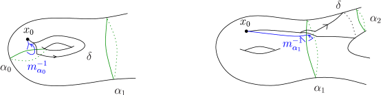
Figure 2: Homotopy classes of meridians.

If $\alpha=\alpha_{0}$ is a pants curve which is not shared by another pair of pants, as on the left in Figure 2, then it has a dual curve $\delta$ which intersects it only once and intersects none of the other curves in $\underline{\alpha}$. Hence:

$$\tau_{*}(\delta)=m_{{\alpha}}^{-1}\cdot\delta.$$

Then for any cocycle $z\in Z^{1}(M;Ad\rho_{0})$, we have

$$z(m_{\alpha}\cdot\tau_{*}(\delta))=z(m_{\alpha})+Ad\rho_{0}(m_{\alpha})z(\tau_{*}(\delta))=z(\delta).$$

Since $z(\delta)$ and $z(\tau_{*}(\delta))$ are both zero by assumption, it must be that $z(m_{\alpha})$ is also zero.

The other possibility for a pants curve ${\alpha}$ of $Q_{0}$ is that it is shared by an adjacent pair of pants, such as ${\alpha}_{1}$ on the right in Figure 2. Such an ${\alpha}$ has a dual curve $\delta$ which intersects it exactly twice and intersects none of the other curves in $\underline{\alpha}$. In particular, we can choose $\delta$ to be freely homotopic to a pants curve in the adjacent pants. Hence, we have the relation

$$\tau_{*}(\delta)=m_{\alpha}^{-1}\cdot\delta\cdot m_{\alpha}$$

from which we obtain

$$z(\delta\cdot m_{\alpha})=z(\delta)+Ad\rho_{0}(\delta)z(m_{\alpha})$$

$$= z(m_{\alpha}\cdot\tau_{*}(\delta))=z(m_{\alpha})+Ad\rho_{0}(m_{\alpha})z(\tau_{*}(\delta)).$$

Since $z(\delta)$ and $z(\tau_{*}(\delta))$ are both zero by hypothesis, $z(m_{\alpha})$ must be contained in the centralizer of $\rho_{0}(\delta)$. On the other hand, since $m_{\alpha}$ and ${\alpha}$ commute, $z(m_{{\alpha}})$ is also in the centralizer of $\rho_{0}({\alpha})$. However, since $\rho_{0}({\alpha})$ and $\rho_{0}(\delta)$ do not commute, $z(m_{{\alpha}})$ must be zero.

We now proceed by an inductive argument on adjacent pairs of pants. For this purpose, we choose homotopy classes for the meridians in a tree-like fashion, as shown in Figure 3, first focusing on the component $S_{0}$.

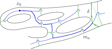
Figure 3: A tree of meridians.

Let ${\alpha}\in\underline{\alpha}$ be the boundary of some pair of pants $Q\subset S_{0}$. Our inductive hypothesis is that there is a chain of pants $Q_{0},Q_{1},\ldots,Q_{j}=Q$ contained in $S_{0}$ such that each meridian associated to a pants curve in $Q_{i}$, $i<j$, has trivial deformation. To show that $z(m_{{\alpha}})=0$, we wish to choose a curve $\delta$ dual to ${\alpha}$ and apply the same argument as before. However, since all loops are based at $x_{0}$, any dual curve is forced to intersect a collection of pants curves. We choose $\delta$ so that it meets a succession of pants curves contained in $\cup_{i\leq j}Q_{i}$, say ${\alpha}_{1},{\alpha}_{2},\ldots,{\alpha}_{k}$ as indicated in the figure. Then

$$\tau_{*}(\delta)=m_{{\alpha}_{1}}^{-1}\cdots m_{{\alpha}_{k}}^{-1}\cdot\delta\cdot m_{{\alpha}_{k}}\cdots m_{{\alpha}_{1}}.$$ (5)

We have that $z(m_{{\alpha}_{1}}),\ldots,z(m_{{\alpha}_{k-1}})$ are zero by the inductive hypothesis and that $z(\tau_{*}(\delta)),z(\delta)$ are zero by the underlying assumption. Denote the product $m_{{\alpha}_{k-1}}\cdots m_{{\alpha}_{1}}$ by $x$. Then Equation(5) gives $x\cdot\tau_{*}(\delta)\cdot x^{-1}=m_{{\alpha}_{k}}^{-1}\cdot\delta\cdot m_{{\alpha}_{k}}$ which implies that $z(m_{{\alpha}_{k}}^{-1}\cdot\delta\cdot m_{{\alpha}_{k}})=0$, and hence $z(m_{{\alpha}_{k}})=Ad\rho_{0}(\delta)z(m_{{\alpha}_{k}}).$ For the same reason as before, $z(m_{{\alpha}_{k}})=z(m_{\alpha})$ is zero. Thus we have shown that $z(m_{\alpha})=0$ for all $\alpha$ in $S_{0}$.

The same method can be used to show that $z(m_{{\alpha}})$ is zero for all ${\alpha}$ in any other component $S$ of $\partial\bar{N}$. Choose a pair of pants $Q$ in $S$ and fix a point $x_{1}$ in $Q$. Let $s$ be an arc in $N$ from $x_{1}$ to $x_{0}$. If ${\beta}$ is a loop based at $x_{1}$, then the concatenation $s*{\beta}*s^{-1}$ is a loop based at $x_{0}$. We can now repeat the previous arguments using loops of this form. Observe that for each pants curve ${\alpha}_{j}$ in $Q$, the loop $\kappa=s*\tau(s)^{-1}$ satisfies the relation

$$\tau_{*}({\alpha}_{j})=\kappa^{-1}\cdot{\alpha}_{j}\cdot\kappa$$

This implies that $z(\kappa)=0$. Using this fact, we can show that $z(m_{{\alpha}_{j}})=0$ for the pants curves ${\alpha}_{j}$ in $Q$ and then apply the inductive argument. In place of Equation(5) we have relations of the form

$$\tau_{*}(\delta)=\kappa^{-1}\cdot m_{{\alpha}_{1}}^{-1}\cdots m_{{\alpha}_{k}}^{-1}\cdot\delta\cdot m_{{\alpha}_{k}}\cdots m_{{\alpha}_{1}}\cdot\kappa.$$

However, since $z(\kappa)=0$, the calculations are identical.  q.e.d.

The following proposition, which exploits the symmetry between $N$ and $\hat{N}$, now completes the proof of Theorem 5.1. Denote by $\mathcal{C}(M,\underline{\alpha})$ the space of cone structures on $M$ with singularities along $\underline{\alpha}$. We also write $\mu_{{\alpha}}$ for the complex length ${\lambda}(\rho(m_{{\alpha}}))$ of the meridian $m_{{\alpha}}$. The crucial observation is that since $\mathcal{C}(M,\underline{\alpha})$ is the purely imaginary locus of the coordinate functions $\mu_{{\alpha}}$, a holomorphic function on $\mathcal{R}(M)$ is locally determined by its values on $\mathcal{C}(M,\underline{\alpha})$.

Proposition 5.3

Let $\sigma_{0}$ be a convex structure in $\mathcal{P}(N,\underline{{\alpha}})$ and let $\rho_{0}$ be its double. Then in a neighborhood of $(r(\rho_{0}),\hat{r}(\rho_{0}))$, the projection ${\mathcal{R}}(N)\times{\mathcal{R}}({\hat{N}})\rightarrow{\mathcal{R}}(N)$ is injective on the image $(r,\hat{r})({\mathcal{R}}(M))$.

Proof. Lifting $\rho_{0}$ to an element in $\mbox{Hom}(M,SL(2,{\mathbb{C}}))$, from the construction in Proposition 2.8, we have $\rho_{0}\circ\tau_{*}=J\rho_{0}J^{-1}$, where $J$ is a reflection in a plane in ${\mathbb{H}}^{3}$. By considering first the reflection induced by $J_{0}(z)=\bar{z}$, it is easy to check that $\mathop{\rm Tr}JAJ^{-1}=\mathop{\rm Tr}\overline{A}$ for any orientation reversing isometry $J$ of ${\mathbb{H}}^{3}$ and $A\in SL(2,{\mathbb{C}})$. Thus $\mathop{\rm Tr}\rho_{0}\circ\tau_{*}(\gamma)=\mathop{\rm Tr}\overline{\rho_{0}(\gamma)}$ for all $\gamma\in\pi_{1}(M)$, where $\overline{A}$ is the matrix whose entries are complex conjugates of those of $A$. Let $\overline{\rho_{0}}$ be the representation defined by $\overline{\rho_{0}}(\gamma)=\overline{\rho_{0}(\gamma)}$. This shows that the two representations $\rho_{0}\circ\tau_{*}$ and $\overline{\rho_{0}}$ are conjugate and thus are equivalent in ${\mathcal{R}}(M)$, see for example [9]. The main point of the proof is to show that for all cone structures $\rho$ near $\rho_{0}$, we have

$$\rho\circ\tau_{*}=\overline{\rho}$$ (6)

as equivalence classes in ${\mathcal{R}}(M)$, where $\overline{\rho}(\gamma)=\overline{\rho(\gamma)}$.

First consider the generic case where $\rho_{0}({\alpha})$ are loxodromic for all ${\alpha}\in\underline{\alpha}$. Then, by Theorem 3.3, a holomorphic deformation of $\rho_{0}$ is parameterized by the complex lengths $\mu_{j}$ of the meridians $m_{j}$, $j=1,\ldots,d$. We shall show below that

$$\mu_{j}(\rho\circ\tau_{*})=\mu_{j}(\bar{\rho}),$$ (7)

for all $j=1,\ldots,d$ and $\rho\in{\mathcal{C}}(M,\underline{\alpha})$ near $\rho_{0}$, which implies Equation(6).

Let ${\alpha},m\in\pi_{1}(M)$ be commuting representatives of a longitude and meridian pair ${\alpha}_{j},m_{j}$. Following the discussion in Section 3.1, in order to compute the complex length $\mu_{{\alpha}}$ of $\rho(m)$, we first conjugate $\rho$ so that the axis of the longitude $\rho({{\alpha}})$ is in standard position, meaning that its repelling and attracting fixed points are at $0,\infty$, respectively. The matrix $A=\rho(m)$ is then diagonal and $\mu_{{\alpha}}(\rho)$ is the logarithm of the top left entry. Now consider the representation $\bar{\rho}$. Notice that when $\rho$ is conjugated so that $\rho({{\alpha}})$ is in standard position, so is ${\bar{\rho}}({\alpha})$. We can therefore read off the complex length $\mu_{{\alpha}}({\bar{\rho}})$ of ${\bar{\rho}}(m)$ from the matrix $\bar{A}=\overline{\rho(m)}$ (see Cases 1 and 2 in Section 3.1). We deduce that $\mu_{j}(\bar{\rho})=\overline{\mu_{j}(\rho)}$ for all $j=1,\ldots,d$. On the other hand, since $\tau_{*}(m)$ is conjugate to $m^{-1}$ in $\pi_{1}(M)$ by the same element which conjugates $\tau_{*}({\alpha})$ to ${\alpha}$, we can use the same method to also deduce that $\mu_{j}(\rho\circ\tau_{*})=-\mu_{j}(\rho).$ Now for $\rho\in{\mathcal{C}}(M,\underline{\alpha})$, the functions $\mu_{j}(\rho)$ are purely imaginary so that $\overline{\mu_{j}(\rho)}=-\mu_{j}(\rho)$. The three equalities give Equation(7) as desired.

We must also consider the case in which some of the meridians are parabolic. For these meridians, the parameter in question is their trace. Note that

$$\mathop{\rm Tr}\rho(m_{j})=\mathop{\rm Tr}\rho(m_{j}^{-1})=\mathop{\rm Tr}\rho\circ\tau_{*}(m_{j}),$$

and

$$\mathop{\rm Tr}\bar{\rho}(m_{j})=\overline{\mathop{\rm Tr}\rho(m_{j})}.$$

In particular, $\mathop{\rm Tr}\rho\circ\tau_{*}(m_{j})={\mathop{\rm Tr}\bar{\rho}(m_{j})}$ whenever $\mathop{\rm Tr}\rho(m_{j})\in{\mathbb{R}}$. (Notice we do not need to assume that all manifolds $\mathop{\rm Tr}\rho(m_{j})\in{\mathbb{R}}$ are cone manifolds; in fact the meridian $\rho(m_{j})$ will be purely hyperbolic for some points in the real trace locus near the parabolic point.)

In summary, if we take local coordinates $w_{j}(\rho)=\mathop{\rm Tr}\rho(m_{j})$ whenever $\rho_{0}(m_{j})$ is parabolic and $w_{j}(\rho)=\sqrt{-1}\mu_{j}(\rho)$ otherwise, we have shown in the two cases above that for all $j=1,\ldots,d$

$$w_{j}(\rho\circ\tau_{*})=w_{j}(\overline{\rho})$$ (8)

on the $d$-dimensional real submanifold of ${\mathcal{R}}(M)$ locally defined by the condition $(w_{1},\ldots,w_{d})\in{\mathbb{R}}^{d}$. Since the map $\rho\mapsto\rho\circ\tau_{*}$ is holomorphic in $\rho$, this implies that for a holomorphic deformation $\rho_{t}$ of $\rho_{0}$, where $t$ is a complex variable in a neighborhood of $0$, we have

$$[\rho_{t}\circ\tau_{*}]=[\overline{\rho_{\overline{t}}}]$$ (9)

as equivalence classes in ${\mathcal{R}}(M)$. (Since we are concerned with deformations only up to first order, we are assuming here that $t$ is real if and only if $w_{j}(t)$ is real, for all $j$.)

We now wish to equate the cocycles defined by the two deformations. Recall that we are identifying the cohomology group $H^{1}(\pi_{1}(M);Ad\,\rho)$ with the holomorphic tangent space to ${\mathcal{R}}(M)$ at $\rho$. In particular, this means that

$$\rho_{t}(\gamma)=\left(Id+t\dot{\rho}(\gamma)+O(|t|^{2})\right)\rho_{0}(\gamma)$$

where $\dot{\rho}=z\in Z^{1}(\pi_{1}(M);Ad\,\rho_{0})$ is the cocycle defined by

$$z(\gamma)=\ \frac{d}{dt}\Big{|}_{t=0}\rho_{t}(\gamma)\rho_{0}(\gamma)^{-1}.$$

Therefore,

$$\overline{\rho_{{\overline{t}}}}(\gamma)=\left(Id+t\overline{\dot{\rho}(\gamma)}+O(|t|^{2})\right)\overline{\rho_{0}}(\gamma).$$

In other words, the cocycle $w$ associated to $\overline{\rho_{\overline{t}}}$ has values given by $w(\gamma)=\overline{z(\gamma)}$. We emphasize that if $z$ is a cocycle in $Z^{1}(\pi_{1}(M);Ad\,{\rho_{0}})$, then the function $\bar{z}$ whose values are given by $\bar{z}(\gamma)=\overline{z(\gamma)}$, is naturally a cocycle in $Z^{1}(\pi_{1}(M);Ad\,\overline{\rho_{0}})$.

On the other hand, the cocycle associated to $\rho_{t}\circ\tau_{*}$ is given by

$$\frac{d}{dt}\Big{|}_{t=0}\rho_{t}(\tau_{*}(\gamma))\rho_{0}(\tau_{*}(\gamma))^{-1}=z(\tau_{*}(\gamma)).$$

Again, note that $z\circ\tau_{*}$ is naturally a cocycle in $Z^{1}(\pi_{1}(M);Ad\,\overline{\rho_{0}})$.

Thus, it follows from Equation(9) that ${z\circ\tau_{*}}$ and $\overline{z}$ differ by a coboundary in $B^{1}(\pi_{1}(M);Ad\,\overline{\rho_{0}})$. In other words, for all $\gamma\in\pi_{1}(M)$, we have

$${z(\tau_{*}(\gamma))}=\overline{z(\gamma)}+v-Ad\,\overline{\rho_{0}}(\gamma)v$$

where $v$ is some element in ${\mathchoice{\hbox{\gthfont s}}{\hbox{\gthfont s}}{\hbox{\smallgthfont s}}{\hbox{\tinygthfont s}}}{\mathchoice{\hbox{\gthfont l}}{\hbox{\gthfont l}}{\hbox{\smallgthfont l}}{\hbox{\tinygthfont l}}}(2,{\mathbb{C}})$. Hence, if $z(\gamma)=0$ for all $\gamma\in\pi_{1}(N)$, it follows that

$$z(\tau_{*}(\gamma))={v}-Ad\overline{\rho_{0}(\gamma)}{v}={v}-Ad{\rho_{0}(\tau_{*}(\gamma))}{v},$$

i.e. $z(\hat{\gamma})={v}-Ad{\rho_{0}(\hat{\gamma})}{v}$ for all $\hat{\gamma}\in\pi_{1}(\hat{N})$.  q.e.d.

This concludes the proof of the local isomorphism theorem 5.1.

We single out the following useful fact extracted from the above proof, see also [31] Section 3.

Corollary 5.4

Let ${\sigma}_{0}$ be a convex structure in ${\mathcal{P}}(N,\underline{\alpha})$ and let $\rho_{0}$ be its double. Then there is a neighborhood $U$ of $\rho_{0}$ in $\mathcal{C}(M,\underline{\alpha})$ such that $\rho\circ\tau_{*}=\bar{\rho}$ for all $\rho\in U$. In particular, $\mathop{\rm Tr}\rho(\gamma)=\overline{\mathop{\rm Tr}\rho(\gamma)}$ whenever $\gamma$ is freely homotopic to a curve on ${\partial}\bar{N}$.

6 Lengths are parameters

6.1 Local parameterization of ${\mathcal{R}}(N)$

We begin by proving the local parameterization theorem, Theorem C. To make a precise statement, we first clarify the definition of the complex length map $\mathcal{L}:{\mathcal{R}}(N)\rightarrow{\mathbb{C}}^{d}$. Let $\underline{\alpha}=\{{\alpha}_{1},\ldots,{\alpha}_{d}\}$ be a maximal doubly incompressible curve system on ${\partial}\bar{N}$ and let ${\sigma}_{0}\in{\mathcal{P}}(N,\underline{\alpha})$ be a convex structure. Number the curves in $\underline{\alpha}$ so that ${\sigma}_{0}({\alpha}_{i})$ is parabolic for $i=1,\ldots,k$ and purely hyperbolic otherwise. Define

$${\mathcal{L}}(\sigma)=(\mathop{\rm Tr}{\sigma}({\alpha}_{1}),\ldots,\mathop{\rm Tr}{\sigma}({\alpha}_{k}),{\lambda}_{{\alpha}_{k+1}}({\sigma}),\ldots,{\lambda}_{{\alpha}_{d}}({\sigma})),$$

where ${\lambda}_{{\alpha}_{i}}({\sigma})$ denotes the complex length ${\lambda}({\sigma}({\alpha}_{i}))$. We can then state Theorem C as:

Theorem 6.1

Let $\underline{\alpha}$ be a maximal curve system on ${\partial}\bar{N}$ and let ${\sigma}_{0}\in{\mathcal{P}}(N,\underline{\alpha})$ be a convex structure. Then ${\mathcal{L}}:{\mathcal{R}}(N)\rightarrow{\mathbb{C}}^{d}$ is a local holomorphic bijection in a neighborhood of $\sigma_{0}$.

We will actually show:

Theorem 6.2

The composition ${\mathcal{L}}\circ r:{\mathcal{R}}(M)\rightarrow{\mathbb{C}}^{d}$ is a local holomorphic bijection in a neighborhood of the double $\rho_{0}$ of ${\sigma}_{0}$, where $r:{\mathcal{R}}(M)\rightarrow{\mathcal{R}}(N)$ is the restriction map.

Combined with Theorem 5.1, this second result gives Theorem 6.1.

Recall that ${\sigma}_{0}({\alpha}_{i})$ is parabolic if and only if $\rho_{0}(m_{i})$ is parabolic for the associated meridian $m_{i}$. (As usual, we use ${\sigma}({\alpha}_{i})$ to mean ${\sigma}(\gamma)$ for $\gamma\in\pi_{1}(N)$ freely homotopic to ${\alpha}_{i}$.) Theorem 3.3 implies that $(z_{1},\dots,z_{d})$ are local coordinates for ${\mathcal{R}}(M)$ near $\rho_{0}$, where $z_{i}=\mathop{\rm Tr}\rho(m_{i})$ for $i\leq k$ and $z_{i}={\lambda}_{m_{i}}(\rho)={\lambda}(\rho(m_{i}))$ for $i>k$. Split the Jacobian of ${\mathcal{L}}\circ r$ at $\rho_{0}$ into four blocks by cutting the matrix between the rows $k,k+1$ and between the columns $k,k+1$. Let $m=d-k$. Proposition 3.5 says that the lower off-diagonal block of size $m\times k$ is the $0$-matrix and that the $k\times k$ block $\left({\partial}\mathop{\rm Tr}r(\rho)({\alpha}_{i}))/{\partial}\mathop{\rm Tr}\rho(m_{j})\right)$ is a diagonal matrix none of whose diagonal entries vanish. Therefore, to show that the Jacobian is non-singular, it is sufficient to show that the $m\times m$ block ${\mathcal{J}}=\left({\partial}{\lambda}_{{\alpha}_{i}}(r(\rho))/{\partial}{\lambda}_{m_{j}}(\rho)\right)$ is non-singular.

Observe that ${\mathcal{J}}$ is the Jacobian of the map $F:{\mathcal{R}}_{P}(M)\rightarrow{\mathbb{C}}^{m}$ defined by

$$F(\rho)=({\lambda}_{{\alpha}_{k+1}}(r(\rho)),\ldots,{\lambda}_{{\alpha}_{d}}(r(\rho))),$$

where ${\mathcal{R}}_{P}(M)$ is the set representations $\rho$ for which $\rho(m_{i})$ is parabolic for $i\leq k$. (By Theorem 3.3, ${\mathcal{R}}_{P}(M)$ is a smooth complex manifold of dimension $m$ near $\rho_{0}$ parameterized by the complex lengths $({\lambda}_{m_{k+1}}(\rho),\ldots,{\lambda}_{m_{d}}(\rho))$.) Clearly $F$ is the composition ${\mathcal{L}}_{m}\circ r_{P}$ of the restriction map $r_{P}:{\mathcal{R}}_{P}(M)\rightarrow{\mathcal{R}}_{P}(N)$ and ${\mathcal{L}}_{m}:{\mathcal{R}}_{P}(N)\rightarrow{\mathbb{C}}^{m}$, where ${\mathcal{L}}_{m}({\sigma})=({\lambda}_{{\alpha}_{k+1}}({\sigma}),\ldots,{\lambda}_{{\alpha}_{d}}({\sigma}))$.

The crucial observation is that $F$ is a ‘real map’ with respect to the two totally real $m$-submanifolds $\mathcal{C}\cap{\mathcal{R}}_{P}(M)$ in the domain and ${\mathbb{R}}^{m}$ in the range, where ${\mathcal{C}}={\mathcal{C}}(M,\underline{\alpha})$ denotes the cone structures in ${\mathcal{R}}(M)$ with singular locus $\underline{\alpha}$. This is where both the local pleating theorem 4.2 and the local isomorphism theorem 5.1 are used:

Proposition 6.3

There is an open neighborhood $V$ of $\rho_{0}$ in $\mathcal{R}_{P}(M)$ such that $F(V\cap{\mathcal{C}(M,\underline{\alpha})})$ is contained in ${\mathbb{R}}^{m}$; and there is an open neighborhood $U$ of $F(\rho_{0})$ in ${\mathbb{C}}^{m}$ such that $F^{-1}(U\cap{\mathbb{R}}^{m})$ is contained in ${\mathcal{C}}(M,\underline{\alpha})$.

Proof. The first statement is immediate from Corollary 5.4. By the local pleating theorem 4.2, there is a neighborhood $W$ of $F(\rho_{0})$ in ${\mathbb{C}}^{m}$ such that ${\mathcal{L}}^{-1}({\mathbb{R}}^{m}\cap W)$ is contained in $\mathcal{G}(N,\underline{\alpha})$. Now for each structure $\sigma\in{\mathcal{L}}^{-1}({\mathbb{R}}^{m}\cap W)$ near $\sigma_{0}$, there is a cone structure $\rho\in{\mathcal{C}}(M,\underline{{\alpha}})$ near $\rho_{0}$ such that $r(\rho)=\sigma$, namely, its double. One deduces easily from Theorem 5.1 that the restriction $r:{\mathcal{R}}(M)\rightarrow{\mathcal{R}}(N)$ induces a local isomorphism $r:{\mathcal{R}}_{P}(M)\rightarrow{\mathcal{R}}_{P}(N)$ in a neighborhood of $\rho_{0}$. It follows that we can find a neighborhood $U$ of $\sigma_{0}$ in ${\mathcal{R}}_{P}(N)$ such that $r^{-1}(\mathcal{G}(N,\underline{{\alpha}})\cap U)\subset{\mathcal{C}}(M,\underline{{\alpha}})$. The result follows. q.e.d.

We complete the proof of Theorem 6.2 using a result from complex analysis. If $H:{\mathbb{C}}\to{\mathbb{C}}$ is a holomorphic map in one variable such that $H(0)=0$, $H({\mathbb{R}})\subset{\mathbb{R}}$ and $H^{-1}({\mathbb{R}})\subset{\mathbb{R}}$, then it is easy to see that $H$ is non-singular at $0$. The following shows that this result extends to holomorphic maps of ${\mathbb{C}}^{m}$.

Proposition 6.4

Let $Z,W$ be open neighborhoods of ${\bf 0}\in{\mathbb{C}}^{m}$ and suppose that $H:Z\to W$ is a holomorphic map such that $H({\bf 0})={\bf 0}$, $H(Z\cap{\mathbb{R}}^{m})\subset{\mathbb{R}}^{m}$ and $H^{-1}(W\cap{\mathbb{R}}^{m})\subset{\mathbb{R}}^{m}$. Then $H$ is invertible on a neighborhood of ${\bf 0}$.

Proof. We will prove that $\mbox{d}H$ is non-singular at ${\bf 0}$. The key is that $H$ cannot be branched and therefore must be one-to-one.

Take coordinates $(z_{i})$ for $Z$ and $(w_{i})$ for $W$. First consider the complex variety $H^{-1}\{{\bf 0}\}$. By hypothesis, it is contained in ${\mathbb{R}}^{m}$. This is not possible unless $H^{-1}\{{\bf 0}\}$ is a variety of dimension $0$, i.e., a discrete subset of points, for otherwise, the coordinate functions $(z_{i})$ would be real-valued on the complex variety $H^{-1}\{{\bf 0}\}$. In this case, $H$ is said to be light at ${\bf 0}$ and there are open neighborhoods ${\tilde{U}}$ of ${\bf 0}$ in the domain and $U$ of ${\bf 0}$ in the range such that the restriction $H|_{\tilde{U}}:{\tilde{U}}\rightarrow U$ is a finite map (see [24], Section V.2.1). Furthermore, by Remmert’s Open Mapping Theorem, $H$ is an open map.

If $\mbox{d}H({\bf 0})$ is singular, then the matrix $\left(\frac{\partial w_{i}}{\partial z_{j}}({\bf 0})\right)$ is singular. Let $u_{i}=\mbox{Re}\,w_{i}$ and $x_{i}=\mbox{Re}\,z_{i}$. Since $H(\tilde{U}\cap{\mathbb{R}}^{m})\subset{\mathbb{R}}^{m}$ it follows that $\frac{\partial u_{i}}{\partial x_{j}}({\bf 0})\in{\mathbb{R}}$. Moreover $\frac{\partial w_{i}}{\partial z_{j}}({\bf 0})=\frac{\partial w_{i}}{\partial x_{j}}({\bf 0})=\frac{\partial u_{i}}{\partial x_{j}}({\bf 0})$, and hence the real matrix $A=\left(\frac{\partial u_{i}}{\partial x_{j}}({\bf 0})\right)$ is singular. In particular, there is a real line $\ell$ in ${\mathbb{R}}^{m}$ whose tangent vector is not contained in the image of $A$. Let $D$ denote the corresponding complex line in ${\mathbb{C}}^{m}$. Then $V=H^{-1}(D)\cap{\tilde{U}}$ is a $1$-dimensional complex variety.

Now, using the classical local description of real and complex $1$ dimensional varieties as in [28] Lemma 3.3, we can pick a branch ${\tilde{D}}$ of $V$ which is locally holomorphic to ${\mathbb{C}}$ and such that ${\tilde{D}}\cap{\mathbb{R}}^{m}$ has a single branch locally holomorphic to ${\mathbb{R}}$. Then $h=H|_{\tilde{D}}:{\tilde{D}}\rightarrow D$ is a non-constant holomorphic map from one complex line to another. Since the image of $\mbox{d}h({\bf 0})$ is trivial, $h$ must be a branched covering of degree $k$ with $k>1$. However, by hypothesis, $h^{-1}(\ell)$ is contained in ${\mathbb{R}}^{m}$ and hence ${\tilde{D}}\cap{\mathbb{R}}^{m}$ contains a union of $k$ distinct lines, a contradiction.  q.e.d.

Proof of Theorem 6.2. Proposition 6.3 shows that, after translating origins, the map $F$ satisfies the conditions on $H$ in Proposition 6.4. Since $r$ is a bijection by Theorem 5.1, the result follows.  q.e.d.

This completes the proofs of Theorems 6.1 and 6.2.

6.2 Global parameterization of $\mathcal{P}(N,\underline{\alpha})$

In this last section, we prove the global parameterization Theorems A,B stated in the introduction.

Proposition 6.5

Let $\underline{\alpha}$ be a maximal doubly incompressible curve system. Then there is a unique point $\sigma_{*}$ in $\mathcal{P}(N,\underline{\alpha})$ such that $\theta_{i}=\pi$ for all $i$. For any $\sigma_{0}\in\mathcal{P}(N,\underline{\alpha})$, there is path $\sigma_{t}\in\mathcal{P}(N,\underline{\alpha}),\ t\in[0,1]$ with initial structure $\sigma_{0}$ such that $\sigma_{1}=\sigma_{*}$.

Proof. Since $\underline{\alpha}$ is maximal, it follows from Proposition 2.7 and [20] that there is a unique hyperbolic structure ${\sigma}_{*}$ on $N$ in which all curves in $\underline{\alpha}$ are parabolic and thus where all bending angles are $\pi$.

Let $\sigma_{0}\in{\mathcal{P}}(N,\underline{\alpha})$ have bending angles $(\theta_{1}{(\sigma_{0})},\ldots,\theta_{n}(\sigma_{0}))$. Suppose first that $\sigma_{0}\in{\mathcal{P}}^{+}(N,\underline{\alpha})$, so that $\theta_{i}{(\sigma_{0})}>0$ for all $i$. By Theorem 1.1 the bending angles parameterize ${\mathcal{P}}^{+}(N,\underline{\alpha})$ and form a convex set. Hence there is a $1$-parameter family of structures ${\sigma}_{t}\in{\mathcal{P}}^{+}(N,\underline{\alpha})$ defined by $\theta_{i}(\sigma_{t})=\theta_{i}(\sigma_{0})+t(\pi-\theta_{i}(\sigma_{0}))$ for each $i$, where $0\leq t\leq 1$. This clearly defines the required path.

Now assume that some of the initial angles vanish. The fact that ${\mathcal{P}}^{+}(N,\underline{\alpha})$ is locally parameterized by the bending angles is deduced from the Hodgson-Kerckhoff theorem (our Theorem 3.3) in Lemme 23 of [5]. We need the extension of this result to ${\mathcal{P}}(N,\underline{\alpha})$. As long as the cone manifold obtained by doubling $N$ has non-zero volume, the Hodgson-Kerckhoff theorem allows that some of the cone angles may be $2\pi$, equivalently that some of the bending angles may vanish. Based on this observation, an inspection of the proof of Lemme 23 shows that the local parameterization for ${\mathcal{P}}^{+}(N,\underline{\alpha})$ goes through unchanged to ${\mathcal{P}}(N,\underline{\alpha})$. In other words, the bending angles are local parameters in a neighborhood of ${\sigma}_{0}$. Therefore, regardless of whether some initial bending angles are zero, there is a small interval $[0,\epsilon]$ for which the structures ${\sigma}_{t}$, $t\in[0,\epsilon]$ are uniquely determined by ${\sigma}_{0}$ and are contained in ${\mathcal{P}}(N,\underline{\alpha})$. Since $\theta_{i}({\sigma}_{\epsilon})>0$ for all $i$, we are now in the situation in which Theorem 1.1 applies and we proceed as before.  q.e.d.

Proposition 6.6

Suppose that $\underline{\alpha}$ is maximal and that $\sigma_{0}\in\mathcal{P}(N,\underline{\alpha})$. Let $\varphi_{{\alpha}_{j}}=2(\pi-\theta_{j})$ be the cone-angle along ${\alpha}_{j}$. Then the Jacobian matrix

$${\mbox{d}}L(\sigma_{0})=\left(\frac{\partial l_{{\alpha}_{i}}}{\partial\varphi_{{\alpha}_{j}}}(\sigma_{0})\right)$$

is positive definite and symmetric.

Proof. Renumber the curves ${\alpha}$ so that $\sigma_{0}({\alpha}_{i})$ is parabolic for $i=1,\ldots,k$ and purely hyperbolic otherwise and let $\rho_{0}$ be the double of ${\sigma}_{0}$. For nearby $\rho$, take local coordinates $(z_{1},\ldots,z_{d})$ where $z_{i}=\mathop{\rm Tr}\rho(m_{i})$ for $i\leq k$ and $z_{i}={\lambda}_{m_{i}}(\rho)$ otherwise. Likewise, near ${\sigma}_{0}$, take local coordinates $(w_{1},\ldots,w_{d})$ where $w_{i}=\mathop{\rm Tr}{\sigma}({\alpha}_{i})$ for $i\leq k$ and $w_{i}=\lambda_{{\alpha}_{i}}({\sigma})$ otherwise. Although for $i\leq k$, the complex length $\lambda_{{\alpha}_{i}}$ cannot be defined in a neighborhood of $\rho_{0}$, we can always pick a branch of $\lambda_{{\alpha}_{i}}$ so that on $\mathcal{P}(N,\underline{\alpha})$ it is a non-negative real valued function $l_{{\alpha}_{i}}$, coinciding with the hyperbolic length of ${\alpha}_{i}$. In Theorem 6.1 we showed that the matrix $\mbox{d}{\mathcal{L}}({\sigma}_{0})=\left(\frac{{\partial}w_{i}}{{\partial}z_{j}}({\sigma}_{0})\right)$ is non-singular. To show that $\mbox{d}L({\sigma}_{0})$ is non-singular, we compare the entries of the two matrices.

In Proposition 3.5 we showed that the upper left $k\times k$ submatrix of $\mbox{d}{\mathcal{L}}({\sigma}_{0})$ is diagonal with non-zero entries. In fact, the diagonal entries are strictly negative. We see this as follows. From Lemma 3.6

$$h_{i}(\rho)^{2}(\mathop{\rm Tr}\rho(m_{i})^{2}-4)=(\mathop{\rm Tr}\rho({\alpha}_{i})^{2}-4)$$

for a locally defined holomorphic function $h_{i}(\rho)$ with the property that $h_{i}(\rho_{0})\neq 0$. For cone structures $\rho$ near $\rho_{0}$, it follows from Corollary 5.4 that both $\mathop{\rm Tr}\rho(m_{i})^{2}-4$ and $\mathop{\rm Tr}\rho({\alpha}_{i})^{2}-4$ are real-valued. A careful inspection shows that $\mathop{\rm Tr}\rho(m_{i})^{2}-4$ and $\mathop{\rm Tr}\rho({\alpha}_{i})^{2}-4$ must be of opposite sign, for otherwise, in the limit, $h_{i}(\rho_{0})$ would be real, making the holonomies $\rho_{0}(m_{i})$ and $\rho_{0}({\alpha}_{i})$ parabolic with the same translation direction. However this contradicts the fact that the translation directions are orthogonal, as discussed in the beginning of Case 3 in Section 3.1. Thus for $i\leq k$,

$$\frac{{\partial}w_{i}}{{\partial}z_{i}}(\rho_{0})=\frac{{\partial}\mathop{\rm Tr}\rho({\alpha}_{i})}{{\partial}\mathop{\rm Tr}\rho(m_{i})}\Big{|}_{\rho=\rho_{0}}=h_{i}^{2}(\rho_{0})<0.$$

Since

$$\frac{{\partial}w_{i}}{{\partial}z_{i}}(\rho_{0})=-\frac{\partial l_{{\alpha}_{i}}}{\partial\varphi_{{\alpha}_{i}}}(\sigma_{0}),$$

it follows that the upper left $k\times k$ submatrix of $\mbox{d}L(\sigma_{0})$ is diagonal with strictly positive entries.

Since deformations which keep $\rho(m_{i})$ parabolic also keep $\rho({\alpha}_{i})$ parabolic, for $i\leq k$ and $j>k$ we have

$$\frac{{\partial}w_{i}}{{\partial}z_{j}}(\sigma_{0})=0=\frac{\partial l_{{\alpha}_{i}}}{\partial\varphi_{{\alpha}_{j}}}(\sigma_{0}).$$

For $j\leq k$ and $i>k$ we calculate directly that for points $\sigma\in{\mathcal{P}}(N,\underline{\alpha})$ near $\sigma_{0}$ we have $z_{j}=2\cos\frac{\varphi_{{\alpha}_{j}}}{2}$ so

$$\frac{\partial l_{{\alpha}_{i}}}{\partial\varphi_{{\alpha}_{j}}}=\frac{\partial l_{{\alpha}_{i}}}{\partial z_{j}}\frac{\partial z_{j}}{\partial\varphi_{{\alpha}_{j}}}=-\frac{\partial l_{{\alpha}_{i}}}{\partial z_{j}}\sin\frac{\varphi_{{\alpha}_{i}}}{2}\to 0.$$

Finally, for $i,j>k$, we have $\varphi_{{\alpha}_{j}}=\mbox{Im}\,z_{j}$ and $l_{{\alpha}_{i}}=\mbox{Re}\,w_{i}$. Recall that if $\rho\in{\mathcal{C}}(M,\underline{\alpha})$, then $w_{i}=l_{{\alpha}_{i}}$ at $r(\rho)$. Therefore, for $i,j>k$,

$$\frac{{\partial}w_{i}}{{\partial}z_{j}}(\sigma_{0})=-\sqrt{-1}\frac{\partial l_{{\alpha}_{i}}}{\partial\varphi_{{\alpha}_{j}}}(\sigma_{0}).$$

It follows that the matrix $\mbox{d}L(\sigma_{0})$ is also non-singular.

Now observe that the Schläfli formula for the volume of the convex core [4] gives

$$\mbox{dVol}=-\frac{1}{2}\sum_{i=1}^{n}l_{{\alpha}_{i}}\mbox{d}\varphi_{{\alpha}_{i}}.$$

Thus the matrix $\mbox{d}L(\sigma_{0})$ is the Hessian of the volume function on ${\mathcal{P}}(N,\underline{\alpha})$. This automatically implies the symmetry relation

$$\frac{\partial l_{{\alpha}_{i}}}{\partial\varphi_{{\alpha}_{j}}}=\frac{\partial l_{{\alpha}_{j}}}{\partial\varphi_{{\alpha}_{i}}},$$

for all $i,j>k$.

This discussion shows that when $\sigma=\sigma_{*}$ represents the structure in which all bending angles are $\pi$, the matrix $\mbox{d}L(\sigma_{*})$ is diagonal and that all diagonal entries are strictly positive. In particular, it is positive definite and symmetric. By Proposition 6.5, $\sigma_{*}$ can be connected to any given $\sigma_{0}\in{\mathcal{P}}(N,\underline{\alpha})$ by a path $\sigma_{t}$ in ${\mathcal{P}}(N,\underline{\alpha})$. Since, by the same reasoning as above, $\mbox{d}L(\sigma_{t})$ is non-degenerate along this path, it must remain positive definite, proving our claim.  q.e.d.

Corollary 6.7

Let $\underline{\alpha}=\{{\alpha}_{1},\ldots,{\alpha}_{n}\}$ be any doubly incompressible curve system on $\bar{N}$, not necessarily maximal. Let ${\sigma}_{0}\in{\mathcal{P}}(N,\underline{\alpha})$ and let $\varphi_{{\alpha}_{j}}=2(\pi-\theta_{{\alpha}_{j}})$ be the cone-angle along ${\alpha}_{j}$. Then the matrix

$$\left(\frac{\partial l_{{\alpha}_{i}}}{\partial\varphi_{{\alpha}_{j}}}(\sigma_{0})\right)_{i,j\leq n}$$

is positive definite and symmetric.

Proof. Extend $\underline{\alpha}$ to a maximal system $\underline{\alpha}^{\prime}$ by adding curves $\{{\alpha}_{n+1},\ldots,{\alpha}_{d}\}$. By Proposition 6.6, the enlarged matrix

$$\left(\frac{\partial l_{{\alpha}_{i}}}{\partial\varphi_{{\alpha}_{j}}}(\sigma_{0})\right)_{i,j\leq d}$$

is positive definite and symmetric. Since a symmetric submatrix of a positive definite symmetric matrix is itself positive definite, the claim follows.  q.e.d.

Theorem B (Mixed parameterization) For any ordering of the curves $\underline{\alpha}$ and for any $q$, the map $\sigma\mapsto(l_{\alpha_{1}}({\sigma}),\ldots,l_{\alpha_{q}}({\sigma}),\theta_{\alpha_{q+1}}({\sigma}),\ldots,\theta_{\alpha_{n}}({\sigma}))$ is an injective local diffeomorphism on ${\mathcal{P}}(N,\underline{\alpha})$.

Proof. Corollary 6.7 shows that the map is a local diffeomorphism, so we have only to show it is injective. Suppose there are two points ${\sigma}_{0},{\sigma}_{1}\in{\mathcal{P}}(N,\underline{\alpha})$ such that $l_{{\alpha}_{i}}({\sigma}_{0})=l_{{\alpha}_{i}}({\sigma}_{1})$ for $i\leq q$ and $\theta_{{\alpha}_{i}}({\sigma}_{0})=\theta_{{\alpha}_{i}}({\sigma}_{1})$ for $i>q$. To simplify notation, let $v_{i}=\theta_{{\alpha}_{i}}({\sigma}_{0})$ and $u_{i}=\theta_{{\alpha}_{i}}({\sigma}_{1})$ for all $i=1,\ldots,n$. It follows from Theorem 1.1 that there is a path ${\sigma}_{t}\in{\mathcal{P}}(N,\underline{\alpha})$ joining ${\sigma}_{0},{\sigma}_{1}$ along which the bending angles are $\theta_{{\alpha}_{i}}(t)=tu_{i}+(1-t)v_{i}$ where $0\leq t\leq 1$. (The case where $u_{i}$ or $v_{i}$ is zero can be handled as in the proof of Proposition 6.5.) Note that $\theta_{{\alpha}_{i}}(t)\equiv u_{i}=v_{i}$ when $i>q$.

Along this path we have

$$\frac{d{l_{{\alpha}_{i}}}}{dt}(\sigma_{t})=\sum_{j=1}^{n}\frac{\partial l_{{\alpha}_{i}}}{\partial\theta_{{\alpha}_{j}}}(\sigma_{t})\,\frac{d\theta_{{\alpha}_{j}}}{dt}=\sum_{j=1}^{n}\frac{\partial l_{{\alpha}_{i}}}{\partial\theta_{{\alpha}_{j}}}(\sigma_{t})(u_{j}-v_{j}).$$

If we multiply both sides by $(u_{i}-v_{i})$ and sum over $i$, it follows from Corollary 6.7 that $\sum_{i=1}^{n}(u_{i}-v_{i})\frac{d{l_{{\alpha}_{i}}}}{dt}(\sigma_{t})=\sum_{i=1}^{q}(u_{i}-v_{i})\frac{d{l_{{\alpha}_{i}}}}{dt}(\sigma_{t})<0$. Thus integrating along $\sigma_{t}$ we find $\sum_{i=1}^{q}(u_{i}-v_{i})(l_{{\alpha}_{i}}({\sigma}_{0})-l_{{\alpha}_{i}}({\sigma}_{1}))<0$. But this is impossible, since by our assumption $l_{{\alpha}_{i}}({\sigma}_{0})=l_{{\alpha}_{i}}({\sigma}_{1})$ for all $i\leq q$.  q.e.d.

Theorem A (Length parameterization) Let $L:{\mathcal{P}}(N,\underline{\alpha})\rightarrow{\mathbb{R}}^{n}$ be the map which associates to each structure $\sigma$ the hyperbolic lengths $(l_{{\alpha}_{1}}(\sigma),\ldots,l_{{\alpha}_{n}}({\sigma}))$ of the curves in the bending locus $\underline{\alpha}=\{{\alpha}_{1},\ldots,{\alpha}_{n}\}$. Then $L$ is an injective local diffeomorphism.

Proof. This is a special case of Theorem B.  q.e.d.

Corollary 6.8

If $c_{j}\in[0,\pi]$ for $j>q$, then

$$\{\sigma\in{\mathcal{P}}(N,\underline{\alpha})\,|\,\theta_{j}(\sigma)\equiv c_{j},j>q\}$$

is parameterized by the lengths $l_{{\alpha}_{j}}$ with $j\leq q$.

We finish with a couple of other easy consequences of the positive definiteness of $\mbox{d}L(\sigma)$.

Corollary 6.9

Suppose that $\sigma\in{\mathcal{P}}(N,\underline{\alpha})$. Then for all ${\alpha}_{i}\in\underline{\alpha}$,

$$\frac{\partial l_{{\alpha}_{i}}}{\partial\varphi_{{\alpha}_{i}}}(\sigma)>0.$$

Therefore in the doubled cone manifold $\Delta(\sigma)$, the length of the singular locus is always increasing as a function of the cone angle.

Remark For a general cone-manifold it is not true that the derivative of the length of the singular locus with respect to the cone angle is always strictly positive. For an example in the case of the figure-eight knot complement, see [7].

Corollary 6.10

The volume of the convex core is a strictly concave function on ${\mathcal{P}}(N,\underline{\alpha})$ as a function of the bending angles, with a global maximum at the unique structure for which all the bending angles are $\pi$.

Proof. Let $\sigma_{0}\in{\mathcal{P}}(N,\underline{\alpha})$ and let $\sigma_{t},\ t\in[0,1]$ denote the path of structures corresponding to the bending angles $\theta_{i}(\sigma_{t})=\theta_{i}(\sigma_{0})+b_{i}t$ where $b_{i}=\pi-\theta_{i}(\sigma_{0})$, as in Proposition 6.5. By Schläfli’s formula, along this path we have

$$\frac{d{\rm Vol}}{dt}(\sigma_{t})=\sum_{i=1}^{n}l_{{\alpha}_{i}}(\sigma_{t})\,\frac{d\theta_{i}}{dt}(\sigma_{t})=\sum_{i=1}^{n}b_{i}l_{{\alpha}_{i}}(\sigma_{t})$$

which is strictly positive except at the unique maximal cusp $\sigma_{1}$.

In a similar way, we can construct a linear path $\sigma_{t}$ between $\sigma_{0}$ and any other point $\sigma^{\prime}\in\mathcal{P}(N,\underline{\alpha})$ with angles given by $\theta_{i}(\sigma_{t})=\theta_{i}(\sigma_{0})+c_{i}t$, where $c_{i}=\theta_{i}(\sigma^{\prime})-\theta_{i}(\sigma_{0})$. To prove concavity, we have to show the second derivative is negative. We have:

$$-\frac{d^{2}{\rm Vol}}{{d}t^{2}}(\sigma_{t})=-\frac{d}{dt}\left(\sum_{i=1}^{n}c_{i}l_{{\alpha}_{i}}(\sigma_{t})\right)=-\sum_{i,j=1}^{n}\frac{\partial l_{{\alpha}_{i}}}{\partial\theta_{{\alpha}_{j}}}(\sigma_{t})c_{i}c_{j}=\frac{1}{2}\sum_{i,j=1}^{n}\frac{\partial l_{{\alpha}_{i}}}{\partial\varphi_{{\alpha}_{j}}}(\sigma_{t})c_{i}c_{j}.$$

The expression on the right is the value of the positive definite quadratic form $\mbox{d}L(\sigma_{t})$ evaluated on the vector $(c_{1},\ldots,c_{d})$ and is therefore positive. The claim follows.  q.e.d.

Appendix

Here is the Bonahon-Otal proof of Proposition 2.7. The topological details they omit are explained in Lemma A.1.

Proof of Proposition 2.7. Let $\bar{M}$ be the compact $3$-manifold obtained from the double $D\bar{N}$ by removing disjoint tubular neighborhoods of the curves in $\underline{\alpha}$ and let $M$ be its interior. Lemma A.1 shows that the condition that $\underline{{\alpha}}$ be doubly incompressible with respect to $(\bar{N},{\partial}\bar{N})$ is precisely the condition needed in order to apply Thurston’s hyperbolization theorem for Haken manifolds (as in for example [29] p.52 or [19] Theorem 1.42) to $\bar{M}$. This gives a finite volume complete hyperbolic structure on $M$ in which every boundary component of $\bar{M}$ corresponds to a rank-$2$ cusp.

There is a natural orientation reversing involution $\tau:M\to M$ which interchanges the two copies of $\bar{N}-\underline{\alpha}$. By Mostow rigidity, $\tau$ is homotopic to an isometry, which we again denote by $\tau$. Taking the quotient of $M$ by $\tau$ endows $\bar{N}-\underline{\alpha}$ with a complete hyperbolic metric of finite volume. The boundary of ${\partial}\bar{N}-\underline{\alpha}$ is the fixed point set of $\tau$ and therefore is the union of totally geodesic surfaces. (The fixed point set of an orientation reversing involution of ${\mathbb{H}}^{3}$ is a plane.) Since all curves in $\underline{\alpha}$ are parabolic by construction, we have exhibited a convex structure on $(\bar{N},\underline{\alpha})$.  q.e.d.

Lemma A.1

Let $\bar{N}$ be a compact orientable $3$-manifold whose interior $N$ admits a complete hyperbolic structure. Assume that ${\partial}\bar{N}$ is non-empty and that it contains only surfaces of strictly negative Euler characteristic Let $\underline{{\alpha}}=\{{\alpha}_{1},\ldots,{\alpha}_{n}\}$ be a doubly incompressible curve system on ${\partial}\bar{N}$ and let $M$ be as defined above. Then ${\partial}\bar{M}$ is incompressible in $\bar{M}$ and $\bar{M}$ is irreducible and atoroidal.

Proof. We begin with some notation. For each $i$, let $U_{{\alpha}_{i}}$ be a regular neighborhood of ${\alpha}_{i}$ in ${\partial}\bar{N}$ and let ${\partial}_{0}\bar{N}={\partial}N-\cup_{i}U_{{\alpha}_{i}}$. Let $N^{+}$ be the manifold with boundary obtained by removing, for each $i$, an open regular tubular neighborhood of ${\alpha}_{i}$ from $\bar{N}$ which intersects ${\partial}\bar{N}$ in $U_{{\alpha}_{i}}$. Let $N^{-}=\sigma(N^{+})$. Then $N^{+}$ and $N^{-}$ are both homeomorphic to $\bar{N}$. Clearly we can take $\bar{M}$ to be the union of the images of $N^{+}$ and $N^{-}$ in $M$ glued along ${\partial}_{0}\bar{N}$. We refer to $N^{+}$ and $N^{-}$ as the sides of $M$. The assumption that $N$ is hyperbolic implies that $N^{\pm}$ are irreducible and atoroidal.

First we check that $\bar{M}$ is irreducible. Let $S$ be an embedded sphere in $\bar{M}$. We may assume that $S\cap{\partial}\bar{M}=\emptyset$, since the existence of a collar neighborhood of ${\partial}\bar{M}$ in $\bar{M}$ allows $S$ to be pushed off ${\partial}\bar{M}$ if necessary. Since the manifolds $N^{\pm}$ are irreducible, we need only consider $S$ which intersects ${\partial}_{0}\bar{N}$. Assume that $S$ has been homotoped so that the intersection is transverse. Then $S\,\cap\,{\partial}_{0}\bar{N}$ is a finite union of disjoint circles. Choose an innermost circle $C$, meaning that $C$ is the boundary of a disk $D(C)$ in $S$ such that $\mbox{Int}\,D(C)\,\cap\,{\partial}_{0}\bar{N}=\emptyset$. Then $D(C)$ is completely contained in one side of $\bar{M}$. Since $C\,\cap\,\underline{\alpha}=\emptyset$, the condition (D.2 ), that every essential disk in $\bar{N}$ intersects $\underline{\alpha}$ at least $3$ times, implies that $D(C)$ is not essential. Therefore, $D(C)$ can be homotoped to a disk $D^{\prime}(C)$ in ${\partial}_{0}\bar{N}$ by a homotopy fixing $C$ and then pushed off ${\partial}_{0}\bar{N}$ so that the number of circles in $S\cap{\partial}_{0}\bar{N}$ is reduced by one. By successively applying the above process, we can homotope $S$ so that it no longer intersects ${\partial}_{0}\bar{N}$, which implies that it is contained in one side of $\bar{M}$ and therefore bounds a $3$-ball.

Note that exactly the same arguments show that ${\partial}_{0}\bar{N}$ is incompressible in $\bar{M}$.

Now we check that $\partial\overline{M}$ is incompressible. Recall that the only irreducible orientable $3$-manifold with a compressible torus boundary component is the solid torus. For suppose that a torus boundary component $T$ of an irreducible $3$-manifold $W$ contains a non-trivial loop $C$ that bounds a disk $D$ in $W$. Let $D\times I$ be a product neighborhood of $D$ meeting $\partial W$ in $\partial D\times I$. The $2$-sphere $D\times\{0,1\}\cup\overline{\partial T-\partial D\times I}$ must bound a $3$-ball $B$ in $W$. The $3$-ball cannot contain $D\times I$ since then it would meet $\partial W$ in more than $\overline{T-\partial D\times I}$. Therefore $W$ is the solid torus obtained by attaching $D\times I$ to $B$ along $D\times\{0,1\}$. So, if any component of $\partial\overline{M}$ were compressible, $\overline{M}$ would be a solid torus. Since $\partial_{0}\overline{N}$ is incompressible, it would consist of annuli, contradicting the fact that each of its components has negative Euler characteristic.

Lastly, we check that $\bar{M}$ is atoroidal. Suppose there is a ${\mathbb{Z}}\oplus{\mathbb{Z}}$ subgroup of $\pi_{1}(\bar{M})$ which is non-peripheral. The torus theorem states that either there is an embedded incompressible torus which is not boundary parallel or $\bar{M}$ is a Seifert fibered space, see [3] Theorem 3.4. (Since $M$ is orientable, we do not need to consider Klein bottles.) We claim $\bar{M}$ cannot be Seifert fibered. As noted above, ${\partial}_{0}\bar{N}$ is incompressible in $\bar{M}$. If $\bar{M}$ were Seifert fibered, then ${\partial}_{0}\bar{N}$ would be isotopic to a vertical or horizontal surface, see Theorem VI.34  [18]. In the first case, $N^{+}$ must admit a Seifert fibering, but then ${\partial}N^{+}$ and hence ${\partial}\bar{N}$ would consist of tori. In the second case, each component of $\bar{M}$ cut along ${\partial}_{0}\bar{N}$ is an $I$-bundle, and the original $\bar{N}$ must have contained an annulus which violates condition (D.1 ) or $\bar{N}$ is an $I$-bundle over a pair of pants which violates condition (D.2 ).

Now suppose there is an incompressible torus $T$ embedded in $\bar{M}$. We may assume that $T\cap{\partial}\bar{M}=\emptyset$. Since the manifolds $N^{\pm}$ are atoroidal, we may assume that $T$ intersects ${\partial}_{0}\bar{N}$ and that the intersection is transverse. Then $T\cap{\partial}_{0}\bar{N}$ is a disjoint union of circles. By the same process as above, we can homotope $T$ to eliminate any circles which are trivial in $T$. Since $T$ is a torus, the remaining circles of intersection must all be parallel and non-trivial. Furthermore, since $T$ is incompressible, the circles are also non-trivial in ${\partial}_{0}\bar{N}$. Take two adjacent circles $C,C^{\prime}$. Then the annulus $A$ they bound in $T$ is completely contained in one side of $\bar{M}$. The condition that there are no essential annuli in $\bar{N}$ with boundary in ${\partial}\bar{N}-\underline{\alpha}$ implies that $A$ is not essential. Therefore $A$ can be homotoped into an annulus $A^{\prime}$ in ${\partial}N^{+}$ or ${\partial}N^{-}$ by a homotopy fixing $C,C^{\prime}$. If $A^{\prime}\cap{\partial}({\partial}_{0}\bar{N})=\emptyset$, then $A^{\prime}$ is contained in a component of ${\partial}_{0}\bar{N}$. In this case, $A^{\prime}$ can be pushed off ${\partial}_{0}\bar{N}$, thereby removing the circles of intersection $C$ and $C^{\prime}$. In this way, we can homotope $T$ so that no pair of adjacent circles in ${\partial}_{0}\bar{N}\cap T$ bound an annulus which can be homotoped into a component of ${\partial}_{0}\bar{N}$. Note that we cannot eliminate all the circles in ${\partial}_{0}\bar{N}\cap T$, since this would imply that there is an incompressible torus entirely contained in one side of $\bar{M}$. Also note that ${\partial}_{0}\bar{N}\cap T$ cannot contain only one circle, since ${\partial}N^{\pm}$ separates $\bar{M}$ into two components. Now if $C,C^{\prime}$ are two adjacent circles in ${\partial}_{0}\bar{N}\cap T$, they bound an annulus $A$ homotopic to an annulus $A^{\prime}$ in ${\partial}N^{+}$ such that $A^{\prime}\cap{\partial}({\partial}_{0}\bar{N})\neq\emptyset$. Since no two curves in $\underline{\alpha}$ are freely homotopic to one another, $A^{\prime}\cap{\partial}({\partial}_{0}\bar{N})$ consists of the two boundary curves of $U_{{\alpha}_{i}}$ for some ${\alpha}_{i}\in\underline{\alpha}$. Since this is true of every annulus in $T$, it must be that $T$ is homotopic into ${\partial}\bar{M}$. A short further analysis confirms that since $T$ is embedded, in fact there must be exactly two distinct circles $C,C^{\prime}$ and hence that $T$ is actually parallel to ${\partial}\bar{M}$.  q.e.d.

References

- [1] L. Bers. On moduli of Kleinian groups. Russian Math. Surveys, 29, 88–102, 1974.
- [2] M. Boileau and J. Porti. Geometrization of -orbifolds of cyclic type, Astérisque 272, Soc. Math. de France, 2001.
- [3] F. Bonahon. Geometric structures on -manifolds. In R. Daverman and R. Sher, eds., Handbook of Geometric Topology, 93–164. Elsevier, 2002.
- [4] F. Bonahon. A Schläfli type formula for convex cores of hyperbolic -manifolds. J. Differential Geometry, 50, 24–58, 1998.
- [5] F. Bonahon and J-P. Otal. Laminations mesurées de plissage des variétés hyperboliques de dimension 3. Annals of Math., to appear.
- [6] R. Canary, D. Epstein and P. Green. Notes on notes of Thurston. In D. Epstein, ed., Analytical and Geometric Aspects of Hyperbolic Space, LMS Lecture Notes 111, 3–92. Cambridge University Press, 1987.
- [7] Y. Choi. Positively oriented triangulations on hyperbolic three-manifolds. Topology, 43, 1345–1371, 2004.
- [8] M. Culler. Lifting representations to covering groups. Advances in Math., 59, 64–70, 1986.
- [9] M. Culler and P. Shalen. Varieties of group representations. Annals of Math., 117, 109–146, 1983.
- [10] R. Díaz and C. Series. Examples of pleating varieties for twice punctured tori. Trans. A.M.S., 356, 621–658, 2003.
- [11] D. Epstein and A. Marden. Convex hulls in hyperbolic space, a theorem of Sullivan, and measured pleated surfaces. In D. Epstein, ed., Analytical and Geometric Aspects of Hyperbolic Space, LMS Lecture Notes 111, 112–253. Cambridge University Press, 1987.
- [12] W. Fenchel. Elementary Geometry in Hyperbolic Space. de Gruyter, 1989.
- [13] W. Goldman. Geometric structures and varieties of representations, in W. Goldman and A. Magid eds., “The Geometry of Group Representations”, Contemp. Math. Vol 74 A.M.S. (1998) 169–198.
- [14] W. Goldman. The symplectic nature of fundamental groups of surfaces. Advances in Math., 54, 200–225, 1984.
- [15] M. Hirsch. Differential Topology. Springer Graduate Texts 33, 1997.
- [16] C. Hodgson. Degenerations and regeneration of hyperbolic structures on three-manifolds. Thesis, Princeton University, 1986.
- [17] C. Hodgson and S. Kerckhoff. Rigidity of hyperbolic cone-manifolds and hyperbolic Dehn surgery. J. Differential Geometry, 48:1–59, 1998.
- [18] W. Jaco. Lectures on Three-Manifold Topology. CBMS Regional Conference Series, No. 43, AMS 1977.
- [19] M. Kapovich. Hyperbolic manifolds and discrete groups. Progress in Maths., 183, Birkhäuser 2001.
- [20] L. Keen, B. Maskit and C. Series. Geometric finiteness and uniqueness for groups with circle packing limit sets. J. reine und angewandte Mathematik 436, 209–219, 1993.
- [21] L. Keen and C. Series. Pleating coordinates for the Maskit embedding of the Teichmüller space of punctured tori. Topology, 32:719–749, 1993.
- [22] L. Keen and C. Series. How to bend pairs of punctured tori. In J. Dodziuk and L. Keen, eds., Lipa’s Legacy, Contemp. Math. 211, 359–388. AMS, 1997.
- [23] L. Keen and C. Series. Pleating invariants for punctured torus groups. Topology, 43, 447 – 491, 2004.
- [24] S. Lojasiewicz. Introduction to complex analytic geometry. Birkhäuser, 1991.
- [25] R. Mañé, P. Sad, and D. Sullivan. On dynamics of rational maps. Ann. Sci. Ecole Norm. Sup., 16:193–217, 1983.
- [26] A. Marden. The geometry of finitely generated Kleinian groups. Ann. Math., 99:607-639, 1974.
- [27] K. Matsuzaki, M. Taniguchi. Hyperbolic Manifolds and Kleinian Groups. Oxford University Press, 1998.
- [28] J. Milnor. Singular points of complex hypersurfaces. Annals of Math. Studies 61. Princeton University Press, 1968.
- [29] J. Morgan. Uniformization theorem for Three-Dimensional Manifolds. In J.Morgan and H. Bass, eds., The Smith Conjecture. Academic Press, 1984.
- [30] D. Mumford, C. Series, D. Wright. Indra’s Pearls. Cambridge University Press, 2002.
- [31] J-P. Otal. Sur le coeur convexe d’une variété hyperbolique de dimension 3. Unpublished preprint, 1994.
- [32] C. Series. Limits of quasifuchsian groups with small bending. Duke Mathematical J., to appear; arXiv: math.GT/0209190.
- [33] C. Series. An extension of Wolpert’s derivative formula. Pacific J. Math, 197, 223-239, 2001.
- [34] W. Thurston. Hyperbolic structures on -manifolds III. Preprint 1986; arXiv:math.GT/9801058, 1998.
- [35] W. Thurston. Geometry and Topology of Three-Manifolds. Princeton lecture notes, 1979.
- [36] F. Waldhausen. On irreducible -manifolds which are sufficiently large. Ann. Math, 87, 56–88, 1968.