Feynman diagrams for pedestrians and mathematicians

1. Introduction

1.1. About these lecture notes

For centuries physics was a potent source providing mathematics with interesting ideas and problems. In the last decades something new started to happen: physicists started to provide mathematicians also with technical tools, methods, and solutions. This process seem to be especially strong in geometry and low-dimensional topology. It is enough to mention the mirror conjecture, Seiberg-Witten invariants, quantum knot invariants, etc.

Mathematicians, however, en masse failed to learn modern physics. There seem to be two main obstructions. Firstly, there are few textbooks in modern physics written in terms accessible for mathematicians. Mathematicians and physicists speak two different languages, and a good “physical-mathematical dictionary” is missing. Thus, to learn something from a physical textbook, a mathematician should start from a hard and time-consuming process of learning the physical jargon.

Secondly, mathematicians consider (and often rightly so) many physical methods and results to be non-rigorous and do not consider them seriously. In particular, path integrals still remain quite problematic from a mathematical point of view (due to some usually unclear measure aspects), so mathematicians are reluctant to accept any results obtained by using path integrals. Yet, this technique may be put to good use, if at least as a tool to guess an answer to a mathematical problem.

In these notes I will focus on perturbative expansions of path integrals near a critical point of the action. This can be done by a standard physical technique of Feynman diagrams expansion, which is a useful book-keeping device for keeping track of all terms in such perturbative series. I will give a rigorous mathematical treatment of this technique in a finite dimensional case (when it actually belongs more to a course of multivariable calculus than to physics), and then use a simple “dictionary” to translate these results to a general infinite dimensional case.

As a result, we will obtain a recipe how to write Feynman diagram expansions for various physical theories. While in general an input of such a recipe includes path integrals, and thus is not well-defined mathematically, it may be used purely formally for producing Feynman diagram series with certain expected properties. A usual trick is then to “sweep under the carpet” all references to the underlying physical theory, keeping only the resulting series. Their expected properties often can be proved rigorously, directly from their definition.

I will illustrate these ideas on the interesting example of the Chern-Simons theory, which leads to universal finite type invariants of knots and 3-manifolds.

A word of caution: during the whole treatment I will brush aside all questions of measures, convergence, and such; see the discussion in Section 4.5.

1.2. Basics of classical and quantum field theories

The remaining part of this section is a brief sketch — on the physical level of rigor — of some basic notions and physical jargon used in the quantum field theory (QFT). Its purpose is to give a basic mathematical dictionary of QFT’s and a motivation for our consideration of Gaussian-type integrals in this note. An impatient reader may skip it without much harm and pass directly to Section 2. Good introductions to field theories can be found e.g. in [12], [21]; mathematical overview can be found in [9]; various topological aspects of QFT are well-presented in [23]. Very roughly, by a field theory one usually means the following.

Given a space-time manifold $X$, one considers a space $\mathcal{F}$ of fields, which are functions of some kind on $X$ (or, more generally, sections of bundles on $X$). A Lagrangian $L:\mathcal{F}\to\mathbb{R}$ on $\mathcal{F}$ gives rise to the action functional $S:\mathcal{F}\to\mathbb{R}$ defined by

$$S(\phi)=\int_{X}L(\phi)dx.$$

In classical field theory one studies critical points of the action $S$ (“classical trajectories of particles”). These fields can be found from the variation principle $\delta S=0$, which is simply an infinite-dimensional version of a standard method for finding the critical points of a smooth function $f:\mathbb{R}\to\mathbb{R}$ by solving $\frac{df}{dx}=0$.

In the quantum field theory one considers instead a partition function given by a path integral

(1) $$Z=\int_{\mathcal{F}}e^{ikS(\phi)}\mathcal{D}\phi.$$

over the space of fields, for a constant $k\in\mathbb{R}$ and some formal measure $\mathcal{D}\phi$ on $\mathcal{F}$. This is the point where mathematicians usually stop, since usually such measures are ill-defined. But let this not disturb us.

In the quasi-classical limit $k\to\infty$, the stationary phase method (see e.g. [8] and also Exercise 2.5) states that under some reasonable assumptions about the behavior of $S$ this fast-oscillating integral localizes on the critical points of $S$, so one recovers the classical case.

The expectation value $\langle f\rangle$ of an observable $f:\mathcal{F}\to\mathbb{R}$ is

$$\langle f\rangle=\frac{1}{Z}\int_{\mathcal{F}}\mathcal{D}\phi\ e^{ikS(\phi)}f(\phi).$$

For a collection $f_{1}$, …, $f_{m}$ of observables their correlation function is

$$\langle f_{1},\dots,f_{m}\rangle=\frac{1}{Z}\int_{\mathcal{F}}\mathcal{D}\phi\ e^{ikS(\phi)}\prod_{i=1}^{n}f_{i}(\phi).$$

By solving a theory one usually means a calculation of these integrals or their asymptotics at $k\to\infty$.

Increasingly often, due to a simpler behavior and better convergence properties, one considers instead the Euclidean partition function, equally well encoding physical information (and related to (1) by a certain analytic continuation in the time domain, called Euclidean, or Wick, rotation):

(2) $$Z=\int_{\mathcal{F}}e^{-kS(\phi)}\mathcal{D}\phi.$$

Since at present a general mathematical treatment of path integrals is lacking, we will first consider a finite dimensional case.

1.3. Finite-dimensional version of QFT

Let us take $\mathcal{F}=\mathbb{R}^{d}$ as the space of fields. An action $S$ and observables $f_{i}$ are then just functions $\mathbb{R}^{d}\to\mathbb{R}$. For a constant $k\in\mathbb{R}$, consider the partition function $Z=\int_{\mathbb{R}^{d}}dxe^{-kS(x)}$ and the correlation functions $\langle f_{1},\dots,f_{m}\rangle=Z^{-1}\int_{\mathbb{R}^{d}}dx\ e^{-kS(x)}\prod_{i}f_{i}(x)$. We are interested in the behavior of $Z$ and $\langle f_{1},\dots,f_{m}\rangle$ in the ”quasi-classical limit” $k\to\infty$.

A well-known stationary phase method states that for large $k$ the main contribution to $Z$ and $\langle f_{1},\dots,f_{m}\rangle$ comes from some small neighborhoods of the points $x$ where $\partial S/\partial x=0$. Thus it suffices to study a behavior of $Z$ and $\langle f_{1},\dots,f_{m}\rangle$ near such a point $x_{0}$. Considering the Taylor expansions of $S$ and $f_{i}$ in $x_{0}$ (and noticing that the linear terms in the expansion of $S$ vanish), after an appropriate changes of coordinates we arrive to the following problem: study integrals

$$\int_{\mathbb{R}^{d}}dx\ e^{-\frac{1}{2}\langle x,Ax\rangle+\hbar U(x)}P(x)$$

for some bilinear form $A$, higher order terms $U(x)$, and monomials $P(x)$ in the coordinates $x^{i}$.

Further in these notes we will calculate such integrals explicitly. To keep track of all terms appearing in these calculations, we will use Feynman diagrams as a simple book-keeping device. See the notes of Kazhdan in [9] for a more in-depth treatment.

2. Finite-dimensional Feynman diagrams

2.1. Gauss integrals

Recall a well-known formula for the Gauss integral (obtained by calculating the square of this integral in polar coordinates):

Proposition 2.1.

$$\int_{-\infty}^{\infty}dxe^{-\frac{1}{2}ax^{2}}=\sqrt{\frac{2\pi}{a}}.$$

More generally, let $A=(A_{ij})$ be a real $d\times d$ positive-definite matrix, $x=(x^{1},\dots,x^{d})$ the Euclidean coordinates in $V=\mathbb{R}^{d}$, and $\langle\ ,\ \rangle:(\mathbb{R}^{d})^{*}\times\mathbb{R}^{d}\to\mathbb{R}$ the standard pairing $\langle x_{i},x^{j}\rangle=\delta_{i}^{j}$. Then

Proposition 2.2.

(3) $$Z_{0}=\int_{\mathbb{R}^{d}}dx\ e^{-\frac{1}{2}\langle Ax,x\rangle}=\left(\det\frac{A}{2\pi}\right)^{-\frac{1}{2}}.$$

Indeed, by an orthogonal transformation (which does not change the integral) we can diagonalize $A$ and apply the previous formula in each coordinate.

Remark 2.3.

In a more formal setting, this may be considered as an equality for a positive-definite symmetric operator $A:V\to V^{*}$ from a $d$-dimensional vector space $V$ to its dual (and $\langle\ ,\ \rangle:V^{*}\times V\to\mathbb{R}$). Indeed, $A$ induces $\det A:\Lambda^{d}V\to\Lambda^{d}V^{*}$, so that $\det A\in(\Lambda^{d}V^{*})^{\otimes 2}$ and $(\det A)^{-\frac{1}{2}}\in|\Lambda^{d}V|$. Hence equality (3) with $\mathbb{R}^{d}$ changed to $V$ still makes sense if we consider both sides as elements of $|\Lambda^{d}V|$. In a similar way, for $\mathbb{C}$-valued symmetric operator $A:V\to V^{*}$ with a positive-definite $\text{Im}A$ one has

$${\int_{V}dx\ e^{\frac{i}{2}\langle Ax,x\rangle}=\left(\det\frac{A}{2\pi i}\right)^{-\frac{1}{2}}}$$

where now both sides belong to $|\Lambda^{d}V|_{\mathbb{C}}$.

A more general form of equation (3) is obtained by adding a linear term $-\langle b,x\rangle$ with $b\in(\mathbb{R}^{d})^{*}$ to the exponent: define $Z_{b}$ by

(4) $$Z_{b}=\int dx\ e^{-\frac{1}{2}\langle Ax,x\rangle+\langle b,x\rangle}.$$

Then, by a change $x\to x-A^{-1}b$ of coordinates, we obtain

Proposition 2.4.

(5) $$Z_{b}=\left(\det\frac{A}{2\pi}\right)^{-\frac{1}{2}}e^{\frac{1}{2}\langle b,A^{-1}b\rangle}=Z_{0}e^{\frac{1}{2}\langle b,A^{-1}b\rangle}.$$

Exercise 2.5.

Verify the stationary phase method in the simplest case: use an appropriate change of coordinates to pass

$$\text{from}\quad\int_{\alpha}^{\beta}dx\ e^{k(-\frac{ax^{2}}{2}+bx)}\quad\text{to}\quad\int_{\alpha^{\prime}}^{\beta^{\prime}}dx\ e^{-\frac{x^{2}}{2}}.$$

What happens to a small $\varepsilon$-neighborhood of the critical point $x_{0}=b/a$ under this change of coordinates? Conclude that in the limit $k\to\infty$ integration over a small neighborhood of $x_{0}=b/a$ gives the same leading term in the expansion of this integral in powers of $k$, as integration over the whole of $\mathbb{R}$.

2.2. Correlation functions

The correlators $\langle f_{1},\dots,f_{m}\rangle$ of $m$ functions $f_{i}:\mathbb{R}^{d}\to\mathbb{R}$ (also called $m$-point functions) are defined by plugging the product of these functions in the integrand and normalizing:

(6) $$\langle f_{1},f_{2},\dots,f_{m}\rangle=\frac{1}{Z_{0}}\int dx\ e^{-\frac{1}{2}\langle Ax,x\rangle}f_{1}(x)\dots f_{m}(x).$$

They may be computed using $Z_{b}$. Indeed, notice that

$$\frac{\partial}{\partial b_{i}}\int dx\ e^{-\frac{1}{2}\langle Ax,x\rangle+\langle b,x\rangle}=\int dx\ e^{-\frac{1}{2}\langle Ax,x\rangle+\langle b,x\rangle}x^{i},$$

hence for correlators of any (not necessary distinct) coordinate functions we have

(7) $$\langle x^{i_{1}},\dots,x^{i_{m}}\rangle=\frac{1}{Z_{0}}\partial_{i_{1}}\dots\partial_{i_{m}}Z_{b}\big{|}_{b=0}=\partial_{i_{1}}\dots\partial_{i_{m}}e^{\frac{1}{2}\langle b,A^{-1}b\rangle}\big{|}_{b=0}$$

where we denoted $\partial_{i}=\partial/\partial b_{i}$.

In particular, 2-point functions are given by the Hessian matrix $\frac{\partial^{2}}{\partial b^{2}}(Z_{b}/Z_{0})\big{|}_{b=0}$ with the matrix elements

(8) $$\langle x^{i},x^{j}\rangle=\partial_{i}\partial_{j}e^{\frac{1}{2}\langle b,A^{-1}b\rangle}\big{|}_{b=0}=(A^{-1})_{ij}.$$

Thus the bilinear pairing $\operatorname{Sym}^{2}(V^{*})\to\mathbb{R}$ given by 2-point functions is just the pairing determined by $A^{-1}$. This explains the similarity of our notations for the 2-point functions and $\langle\ ,\ \rangle:V^{*}\times V\to\mathbb{R}$.

For polynomials, or more generally, formal power series $f_{1},\dots,f_{m}$ in the coordinates we may apply (7) (with $i_{1}=i_{2}=\dots=i_{n}=i$ for each monomial $(x^{i})^{n}$) and then put the series back together, noting that each $x^{i}$ should be substituted by $\partial_{i}$. This yields:

Proposition 2.6.

(9) $$\left.\langle f_{1},f_{2},\dots,f_{m}\rangle=f_{1}\left(\frac{\partial}{\partial b}\right)\dots f_{m}\left(\frac{\partial}{\partial b}\right)\,e^{\frac{1}{2}\langle b,A^{-1}b\rangle}\right|_{b=0}$$

2.3. Wick’s theorem

Denote by $A^{ij}$ the matrix elements $(A^{-1})_{ij}$ of $A^{-1}$. The key ingredient of the Feynman diagrams technique is Wick’s theorem (see e.g. [22]) which we state in its simplest form:

Theorem 2.7 (Wick).

(10) $$\partial_{i_{1}}\dots\partial_{i_{m}}e^{\frac{1}{2}\langle b,A^{-1}b\rangle}\big{|}_{b=0}=\begin{cases}\sum A^{j_{1}j_{2}}\dots A^{j_{m-1}j_{m}},\quad m=2n\\ 0,\quad m=2n+1\end{cases}$$

where the sum is over all partitions $(j_{1},j_{2})$,…, $(j_{m-1},j_{m})$ in pairs of the set $i_{1}$,$i_{2}$,…,$i_{m}$ of indices.

Proof.

For each $k$, the expression $\partial_{i_{1}}\dots\partial_{i_{k}}e^{\frac{1}{2}\langle b,A^{-1}b\rangle}$, considered as a function of $b$, is always of the form $P_{i_{1}\dots i_{k}}(b)e^{\frac{1}{2}\langle b,A^{-1}b\rangle}$, where $P_{i_{1}\dots i_{k}}(b)$ is a polynomial. Each new derivative $\partial_{j}$ acts either on the polynomial part, or on the exponent, by the rule

$$\partial_{j}\big{(}P(b)e^{\frac{1}{2}\langle b,A^{-1}b\rangle}\big{)}=\partial_{j}(P(b))e^{\frac{1}{2}\langle b,A^{-1}b\rangle}+P(b)(\sum_{i}A^{ji}b_{i})e^{\frac{1}{2}\langle b,A^{-1}b\rangle},$$

so the polynomial part $P_{i_{1}\dots i_{m}}(b)$ may be defined recursively by $P_{\emptyset}(b)={\bf 1}$ and

(11) $$P_{i_{1}\dots i_{m}}(b)=(\partial_{i_{1}}+\sum_{i}A^{i_{1}i}b_{i})P_{i_{2}\dots i_{m}}(b)=\dots{\\ }=(\partial_{i_{1}}+\sum_{i}A^{i_{1}i}b_{i})\dots(\partial_{i_{m}}+\sum_{i}A^{i_{m}i}b_{i}){\bf 1},$$

where ${\bf 1}$ is the function identically equal to 1. We are interested in the constant term $P_{i_{1}\dots i_{m}}(0)$. Directly from (11) we can make two observations. Firstly, if $m$ is odd, $P_{i_{1}\dots i_{m}}(b)$ contains only terms of odd degrees, in particular $P_{i_{1}\dots i_{m}}(0)=0$. Secondly, unless each derivative $\partial_{i_{k}}$, $k<m$ acts on the term $\sum_{i}A^{i_{l}i}b_{i}$ in some $l$-th, $l>k$, factor of the (11), the evaluation at $b=0$ would give zero. Each such pair $(i_{k},i_{l})$ contributes a factor of $A^{i_{l}i_{k}}$ to the constant term of $P_{i_{1}\dots i_{m}}$. These observations prove the theorem. ∎

It is convenient to extend (10) by linearity to arbitrary linear functions of the coordinates, note that in this case we may define the $2$-point functions $\langle f,g\rangle$ by $\langle f,A^{-1}g\rangle$ in view of (8), and finally combine it with (7) into the following version of Wick’s theorem:

Theorem 2.8 (Wick).

Let $f_{1}(x),\dots,f_{m}(x)$ be arbitrary linear functions of the coordinates $x_{i}$. Then all $m$-point functions vanish for odd $m$. For $m=2n$ one has

(12) $$\langle f_{1},\dots,f_{m}\rangle=\sum\langle f_{i_{1}},f_{i_{2}}\rangle\dots\langle f_{i_{m-1}},f_{i_{m}}\rangle,$$

where the sum is over all pairings $(i_{1},i_{2})$,…, $(i_{m-1},i_{m})$ of $1,\dots,m$ and the $2$-point functions $\langle f_{j},f_{k}\rangle$ are given by $\langle f_{j},A^{-1}f_{k}\rangle$.

Remark 2.9.

Another idea for a proof of Theorem 2.8 is the following. Note that both sides of (12) are symmetric functions of $1,\dots,m$, so they may be considered as functions on $m$-th symmetric power $S^{m}(V)$ of $V=\mathbb{R}^{d}$. Thus it suffices to check (12) only for $f_{1}=\dots=f_{m}=f$; in this case it is obvious.

Exercise 2.10.

Check that the number of all pairings of $1,\dots,2n$ is $(2n)!/2^{n}n!$. Calculate

$$\int_{-\infty}^{\infty}dx\ x^{m}e^{x^{2}/2}$$

using integration by parts and Proposition 2.1. Calculate

$$\left.\frac{d^{m}}{dx^{m}}e^{x^{2}/2}\right|_{x=0}$$

substituting $x^{2}/2$ instead of $x$ in the Taylor series expansion of $e^{x}$. Compare these expressions and explain how are they related to the above number of pairings.

Exercise 2.11.

Find formulas for the 4-point functions $\langle x_{1},x_{1},x_{2},x_{3}\rangle$ and $\langle x_{1},x_{1},x_{1},x_{2}\rangle$.

2.4. First Feynman graphs

It is convenient to represent each term

$$\langle f_{i_{1}},f_{i_{2}}\rangle\dots\langle f_{i_{m-1}},f_{i_{m}}\rangle$$

in Wick’s formula (12) by a simple graph. Indeed, consider $m$ points, with the $k$-th point representing $f_{k}$. A pairing of $1,\dots,2n$ gives a natural way to connect these points by $n$ edges, with an edge (a propagator in the physical jargon) $e=(j,k)$ representing $A^{-1}_{e}=\langle f_{j},A^{-1}f_{k}\rangle$. Equation (12) becomes then

(13) $$\langle f_{1},\dots,f_{m}\rangle=\sum_{\Gamma}\prod_{e\in\text{edges}(\Gamma)}A^{-1}_{e},$$

where the sum is over all univalent graphs as above.

Example 2.12.

An application of equation (13) for $n=2$ (see Figure 1a) gives the following:

$$\langle x_{1},x_{2},x_{3},x_{4}\rangle =A^{12}A^{34}+A^{13}A^{24}+A^{14}A^{23},$$

$$\langle x_{1},x_{1},x_{2},x_{2}\rangle =A^{11}A^{22}+2A^{12}A^{12},$$

$$\langle x_{1},x_{1},x_{1},x_{1}\rangle =3A^{11}A^{11}.$$

2.5. Adding a potential

The above computations may be further generalized by adding a potential function $U(x)$ (with some small parameter $\hbar=k^{-1}$) to $\langle Ax,x\rangle$ in the definition of $Z_{0}$. Namely, define $Z_{U}$ by

(14) $$Z_{U}=\int dx\ e^{-\frac{1}{2}\langle Ax,x\rangle+\hbar U(x)}.$$

Applying (9) for $f=e^{\hbar U(x)}$ we get:

Proposition 2.13.

(15) $$Z_{U}=Z_{0}e^{\hbar U(\frac{\partial}{\partial b})}e^{\frac{1}{2}\langle b,A^{-1}b\rangle}\big{|}_{b=0}.$$

Correlation functions $\langle f_{1},\dots,f_{m}\rangle_{U}$ are defined similarly to (6):

(16) $$\langle f_{1},f_{2},\dots,f_{m}\rangle_{U}=\frac{1}{Z_{U}}\int dx\ e^{-\frac{1}{2}\langle Ax,x\rangle+\hbar U(x)}f_{1}(x)\dots f_{k}(x).$$

Using (9) once again, we get

Proposition 2.14.

(17) $$\langle f_{1},f_{2},\dots,f_{m}\rangle_{U}=\frac{Z_{0}}{Z_{U}}e^{\hbar U(\frac{\partial}{\partial b})}f_{1}\left(\frac{\partial}{\partial b}\right)\dots f_{m}\left(\frac{\partial}{\partial b}\right)\left.e^{\frac{1}{2}\langle b,A^{-1}b\rangle}\right|_{b=0}.$$

2.6. A cubic potential

Consider the important example of a cubic potential function $U(x)=\sum U_{ijk}x^{i}x^{j}x^{k}$. Let us compute the expansion of the partition function (14) in power series in $\hbar$. The coefficient of $\hbar^{n}$ in the expansion of (15) is

$$\frac{Z_{0}}{n!}\left(\sum_{i,j,k}U_{ijk}\partial_{i}\partial_{j}\partial_{k}\right)^{n}\,\left.e^{\frac{1}{2}\langle b,A^{-1}b\rangle}\right|_{b=0}.$$

Let us start with the lowest degrees. By Wick’s theorem, the coefficient of $\hbar$ vanishes and the coefficient of $\hbar^{2}$ is given by

(18) $$\frac{Z_{0}}{2!}\sum_{i,j,k}\sum_{i^{\prime},j^{\prime},k^{\prime}}U_{ijk}U_{i^{\prime}j^{\prime}k^{\prime}}\partial_{i}\partial_{j}\partial_{k}\partial_{i^{\prime}}\partial_{j^{\prime}}\partial_{k^{\prime}}e^{\frac{1}{2}\langle b,A^{-1}b\rangle}\big{|}_{b=0}=\\ \frac{Z_{0}}{2!}\sum_{i,j,k}\sum_{i^{\prime},j^{\prime},k^{\prime}}U_{ijk}U_{i^{\prime}j^{\prime}k^{\prime}}\sum A^{i_{1}i_{2}}A^{i_{3}i_{4}}A^{i_{5}i_{6}},$$

where the last sum is over all pairings $(i_{1},i_{2})$,…,$(i_{5},i_{6})$ of $i,j,k,i^{\prime},j^{\prime},k^{\prime}$. We may again encode these pairings by labelled graphs, connecting 6 vertices labelled by $i,j,k,i^{\prime},j^{\prime},k^{\prime}$ by three edges $(i_{1},i_{2})$,$(i_{3},i_{4})$,$(i_{5},i_{6})$ representing $A^{i_{1}i_{2}}A^{i_{3}i_{4}}A^{i_{5}i_{6}}$. This time, however, we have an additional factor $U_{ijk}U_{i^{\prime}j^{\prime}k^{\prime}}$. To represent $U_{ijk}$ graphically, let us glue the triple $(i,j,k)$ of univalent vertices in a trivalent vertex; to preserve the labels, we can write them on the ends of the edges meeting in this new vertex (i.e., on the star of the vertex). Similarly, we represent $U_{i^{\prime}j^{\prime}k^{\prime}}$ by gluing the remaining triple $(i^{\prime},j^{\prime},k^{\prime})$ of univalent vertices into a second trivalent vertex. Thus for each of the $6!/(2^{3}3!)=15$ pairings of $i,j,k,i^{\prime},j^{\prime},k^{\prime}$ we end up with a graph with two trivalent vertices; we get 6 copies of the $\Theta$-graph and 9 copies of the dumbbell graph shown in Figure 1b.

Figure 1. Terms of $\langle x_{1},x_{2},x_{3},x_{4}\rangle$ and graphs of degree two

Note, however, that each of these labelled graphs is considered up to its automorphisms, i.e. maps of a graph onto itself, mapping edges to edges and vertices to vertices and preserving the incidence relation. Indeed, while the application of an automorphism changes the labels, it preserves their pairing (edges) and the way they are united in triples (vertices), thus corresponds to the same term in the right hand side of (18). Instead of summing over the automorphism classes of graphs, we may sum over all labelled graphs, but divide the term corresponding to a graph $\Gamma$ by the number $|\operatorname{Aut}\Gamma|$ of its automorphisms. E.g., for the $\Theta$-graph of Figure 1b $|\operatorname{Aut}\Gamma|=12$, and twelve copies of this graph (which differ only by transpositions of the labels) all give the same terms $U_{ijk}U_{i^{\prime}j^{\prime}k^{\prime}}A^{ii^{\prime}}A^{jj^{\prime}}A^{kk^{\prime}}$.

Also, when summing the resulting expressions over all indices, note that the terms corresponding to $i,j,k,i^{\prime},j^{\prime},k^{\prime}$ and to $i^{\prime},j^{\prime},k^{\prime},i,j,k$ are the same (which will cancel out with $1/2!$ in front of the sum). Hence, we may write the coefficient of $\hbar^{2}$ in the following form:

$$Z_{0}\sum_{\Gamma}\frac{1}{|\operatorname{Aut}\Gamma|}\sum_{labels}\prod_{v}U_{v}\prod_{e}A^{-1}_{e},$$

Here the sum is over all trivalent graphs with two vertices and labellings of their edges, $U_{v}=U_{ijk}$ for a vertex $v$ with the labels $i,j,k$ of the adjacent edges, and $A^{-1}_{e}=A^{ij}$ for an edge $e$ with labels $i,j$.

Exercise 2.15.

Calculate the number of automorphisms of the dumbbell graph of Figure 1b.

In general, for the coefficient of $\hbar^{n}$ we get the same formula, but with the summation being over all labelled trivalent graphs with $n$ vertices.

2.7. Correlators for a cubic potential

We may treat $m$-point functions in a similar way. Let us first consider the power series expansion in $\hbar$ of $Z_{U}\langle x^{i_{1}},\dots,x^{i_{m}}\rangle_{U}$. The coefficient of $\hbar^{n}$ is

$$\frac{Z_{0}}{n!}\left(\sum_{i,j,k}U_{ijk}\partial_{i}\partial_{j}\partial_{k}\right)^{n}\partial_{i_{1}}\dots\partial_{i_{m}}\,\left.e^{\frac{1}{2}\langle b,A^{-1}b\rangle}\right|_{b=0}.$$

Thus it may again be presented by a sum over labelled graphs, with the only difference being that now in addition to $n$ trivalent vertices these graphs also have $m$ ordered legs (i.e. univalent vertices) labelled by $i_{1},\dots,i_{m}$. See Figure 2 for graphs representing the coefficient of $\hbar^{2}$ in $Z_{U}\langle x^{1},x^{2}\rangle_{U}$.

Figure 2. Degree two graphs with two legs

However, not all of these graphs will enter in the expression for $\langle x^{i_{1}},\dots,x^{i_{m}}\rangle_{U}$, since we should now divide this sum over graphs by $Z_{U}$ (represented by a similar sum, but over graphs with no legs). This will remove all vacuum diagrams, i.e. all graphs which contain some component with no legs. Indeed, the term corresponding to a non-connected graph is a product of terms corresponding to each connected component. Each component with no legs appears also in the expansion of $Z_{U}$ and thus will cancel out after we divide by $Z_{U}$. For example, the first graph of Figure 2 contains a vacuum $\Theta$-graph component. But it also appears in the expansion of $Z_{U}$ (see Figure 1b). Thus the corresponding factor cancels out after division by $Z_{U}$. The same happens with the second graph of Figure 2. As a result, only the last two graphs of Figure 2 will contribute to the coefficient of $\hbar^{2}$ in the expansion of $\langle x^{1},x^{2}\rangle_{U}$.

Example 2.16 (”A finite dimensional $\phi^{3}$-theory”).

Take $U_{ijk}=\delta_{ij}\delta_{jk}$, i.e. $U=\sum_{i}(x^{i})^{3}$. Note that since all ends of edges meeting in a vertex are labelled by the same index, we may instead label the vertices. Thus the calculation rules are quite simple: we count uni-trivalent graphs; a vertex represents a sum $\sum_{i}$ over its labels; an edge with the ends labelled by $i,j$ represents $A^{ij}$. The coefficients of $\hbar^{2}$ in $Z_{U}$ and in $\langle x^{1},x^{2}\rangle_{U}$ are given by

$$Z_{0} \sum_{i,j}6(A^{ij})^{3}+9A^{ij}A^{ii}A^{jj},$$

$$\sum_{i,j}9A^{1i}A^{2j}A^{ii}A^{jj}+6A^{1i}A^{2j}(A^{ij})^{2}$$

respectively. We can identify these terms with two graphs of Figure 1b and two last graphs of Figure 2, respectively. The first two graphs of Figure 2 represent

$$\sum_{i,j}6A^{12}(A^{ij})^{3}+9A^{12}A^{ij}A^{ii}A^{jj}.$$

These terms do appear in the $\hbar^{2}$ coefficient of $Z_{U}\langle x^{1},x^{2}\rangle$, but cancel out after we divide it by $Z_{U}=Z_{0}\big{(}1+\hbar^{2}\sum_{i,j}(6(A^{ij})^{3}+9A^{ij}A^{ii}A^{jj})+\dots\big{)}$.

2.8. General Feynman graphs

It is now clear how to generalize the above results to the case of a general potential $U(x)$: the $k$-th degree term $U_{i_{1}\dots i_{k}}x^{i_{1}}\dots x^{i_{k}}$ of $U$ will lead to an appearance of $k$-valent vertices representing factors $U_{i_{1}\dots i_{k}}$. We will call such a vertex an internal vertex. We assume that there are no linear and quadratic terms in the potential, so further we will always assume that all internal vertices of any Feynman graph $\Gamma$ are of valence $\geq 3$; denote their number by $|\Gamma|$. Denote by $\Gamma^{0}$ the set of all graphs with no legs. Also, for $m\geq 1$, denote by $\Gamma^{m}$ the set of all non-vacuum (i.e. such that each connected component has at least one leg) graphs with $m$ ordered legs.

Denoting $U_{v}=U_{i_{1}\dots i_{k}}$ for an internal vertex $v$ with the labels $i_{1},\dots,i_{k}$ of adjacent edges, and $A^{-1}_{e}=A^{ij}$ for an edge $e$ with its ends labelled by $i,j$, we get

Proposition 2.17.

(19) $$Z_{U}=Z_{0}\sum_{\Gamma\in\Gamma^{0}}\frac{\hbar^{|\Gamma|}}{|\operatorname{Aut}\Gamma|}\sum_{labels}\prod_{v}U_{v}\prod_{e}A^{-1}_{e}.$$

Note that instead of performing the internal summation over all labellings, one may include the summation over labels of the star of a vertex into the weight of this vertex.

In a similar way, for $m$-point functions we get

Proposition 2.18.

For even $m$,

(20) $$\langle x^{i_{1}},\dots,x^{i_{m}}\rangle_{U}=\sum_{\Gamma\in\Gamma^{m}}\frac{\hbar^{|\Gamma|}}{|\operatorname{Aut}\Gamma|}\sum_{labels}\prod_{v}U_{v}\prod_{e}A^{-1}_{e},$$

where the sum is over all labelled graphs $\Gamma$ with $m$ legs labelled by $i_{1},\dots,i_{m}$.

Again, we may include the summation over the labels of the star of an internal vertex into the weight of this vertex.

2.9. Weights of graphs

Let us reformulate the above results using a general notion of weights of graphs.

Let $V$ be a vector space. A weight system is a collection $(a,\{u_{k}\}_{k=3}^{\infty})$ of $a\in\operatorname{Sym}^{2}(V)$ and $u_{k}\in\operatorname{Sym}^{k}(V^{*})$. A weight system $W$ defines a weight $W_{\Gamma}:(V^{*})^{\otimes m}\to\mathbb{R}$ of a graph $\Gamma\in\Gamma^{m}$ in the following way. Assign $u_{k}\in\operatorname{Sym}^{k}(V^{*})$ to each internal vertex $v$ of valence $k$, associating each copy of $V^{*}$ with (an end of) an edge. Also, to the $i$-th leg of $\Gamma$, $i=1,\dots,m$ assign some $f_{i}\in V^{*}$. Now, for each edge contract two copies of $V^{*}$ associated to its ends using $a\in\operatorname{Sym}^{2}(V)$. After all copies of $V^{*}$ get contracted, we obtain a number $W_{\Gamma}(f_{1},\dots,f_{m})\in\mathbb{R}$.

In our case, a bilinear form $A^{-1}$ and a potential $\hbar U(x)$ determine a weight system in an obvious way: set $a=A^{-1}$ and let $u_{v}$ to be the degree $k$ part of $\hbar U(x)$. These rules of computing the weights corresponding to a physical theory are called Feynman rules.

Formulas (19) and (20) above can be reformulated in these terms as

(21) $$Z_{U} =Z_{0}\sum_{\Gamma\in\Gamma^{0}}\frac{1}{|\operatorname{Aut}\Gamma|}W_{\Gamma},$$

$$\langle f_{1},\dots,f_{m}\rangle_{U} =\sum_{\Gamma\in\Gamma^{m}}\frac{1}{|\operatorname{Aut}\Gamma|}W_{\Gamma}(f_{1},\dots,f_{m}).$$

Exercise 2.19 (Finite dimensional $\phi^{4}$-theory).

Consider a potential $U=\sum_{i}(x^{i})^{4}$. Formulate the Feynman rules. Find the graphs which contribute to the coefficient of $\hbar^{2}$ of $Z_{U}$ and compute their coefficients. Do the same for $\langle x^{1},x^{2}\rangle_{U}$. Draw the graph representing $\sum_{i}A^{12}(A^{ii})^{2}$; does it appear in the expansion of $\langle x^{1},x^{2}\rangle_{U}$ and why?

2.10. Free energy: taking the logarithm

The summation in equation (21) is over all graphs in $\Gamma^{0}$, which are plenty. Denote by $\Gamma^{0}_{conn}$ the subset of all connected graphs in $\Gamma^{0}$. There is a simple way to leave only a sum over graphs in $\Gamma^{0}_{conn}$, namely to take the logarithm of the partition function (called the free energy in the physical literature):

Proposition 2.20.

Let $W$ be a weight system. Then

$$\log\left(\sum_{\Gamma\in\Gamma^{0}}\frac{1}{|\operatorname{Aut}\Gamma|}W_{\Gamma}\right)=\sum_{\Gamma\in\Gamma^{0}_{conn}}\frac{1}{|\operatorname{Aut}\Gamma|}W_{\Gamma}.$$

Proof.

Let us compare the terms of the power series expansion for the right hand side with the terms in the left hand side:

$$\exp\left(\sum_{\Gamma\in\Gamma^{0}_{conn}}\frac{1}{|\operatorname{Aut}\Gamma|}W_{\Gamma}\right)=\sum\frac{1}{n_{1}!\dots n_{k}!}W_{\Gamma_{1}}^{n_{1}}\dots W_{\Gamma_{k}}^{n_{k}},$$

where the sum is over all $k$, $n_{i}$, and distinct $\Gamma_{i}\in\Gamma^{0}_{conn}$, $i=1,\dots,k$. Consider $\Gamma=(\Gamma_{1})^{n_{1}}\dots(\Gamma_{k})^{n_{k}}\in\Gamma^{0}$. Since in addition to automorphisms of each $\Gamma_{i}$ there are also automorphisms of $\Gamma$ interchanging the $n_{i}$ copies of $\Gamma_{i}$, we have $|\operatorname{Aut}\Gamma|=n_{1}!\dots n_{k}!|\operatorname{Aut}\Gamma_{1}|\dots|\operatorname{Aut}\Gamma_{k}|$. Also, any weight system satisfies $W_{\Gamma^{\prime}\Gamma^{\prime\prime}}=W_{\Gamma^{\prime}}W_{\Gamma^{\prime\prime}}$, hence $W_{\Gamma}=W_{\Gamma_{1}}^{n_{1}}\dots W_{\Gamma_{k}}^{n_{k}}$. The proposition follows. ∎

Exercise 2.21.

Formulate and prove a similar statement for graphs with legs.

Remark 2.22.

It is possible to restrict the class of graphs to 1-connected (in the physical literature usually called $1$-point irreducible, or 1PI for short) graphs. A graph is 1-connected, if it remains connected after a removal of any one of its edges. This involves a passage to a so-called effective action, which I will not discuss here in details. Mathematically, it simply means an application of a Legendrian transform (a discrete version of a Fourier transform): if $z(b)=\log(Z_{b})$ is given by the sum over all connected graphs as in Proposition 2.20, then $\hat{z}(x)=\langle b,x\rangle-z(b)$ is given by a similar sum over all 1PI graphs (and $b(x)$ may be recovered as $\partial\hat{z}/\partial x$).

3. Gauge theories and gauge fixing

3.1. Gauge fixing

All calculations of the previous section dealt only with the case of a non-degenerate bilinear form $A$; in particular, the critical points of the action $S(x)$ had to be isolated (see Section 1.3). However, gauge theories present a large class of examples when it is not so. Suppose that we have an $l$-dimensional group of symmetries, i.e. the Lagrangian is invariant under a (free, proper, isometric) action of an $l$-dimensional Lie group $G$. Then instead of isolated critical points we have critical orbits, so $A$ has $l$ degenerate directions and the technique of Gauss integration can not be applied.

Let us try to calculate the partition and correlation functions without a superfluous integration over the orbits of $G$. In other words, we wish to reduce integrals of $G$-invariant functions on $X$ to integrals on the quotient space $\widetilde{X}=X/G$ of $G$-orbits. For this purpose, starting from a $G$-invariant measure on $X$ we should desintegrate it as the Haar measure on the orbits over some “quotient measure” $\tilde{\mu}$ on the base $\widetilde{X}$.

If $G$ is compact then $\tilde{\mu}$ is the standard push-forward of $\mu$. For example, if $f$ is a rotationally invariant function on $\mathbb{R}^{2}$, we can take the pair of polar coordinates $(r,\phi)$ as coordinates in the quotient space $\widetilde{X}$ and the orbit, respectively. The measure on $\widetilde{X}$ in this case is $2\pi r\,dr$ and we get the following elementary formula:

$$\int_{\mathbb{R}^{2}}f(|x|)\ d^{2}x=2\pi\int_{0}^{\infty}f(r)r\ dr.$$

If $G$ is a locally compact group acting properly on $X$ then $\tilde{\mu}$ can be defined by the property

$$\mu(Y)=\int_{\widetilde{X}}|Y\cap G(\tilde{x})|\,d\tilde{\mu}(\tilde{x}),$$

where $G(\tilde{x})$ is the fiber over $\tilde{x}\in\widetilde{X}$ and $|\cdot|$ is the Haar measure on it. In this case the integral $\int_{X}f\,dx$ in question is infinite, but it can be formally defined (“regularized”) as $\int_{\tilde{X}}fd\tilde{x}$.

A standard physical procedure for the desintegration that can be applied also to a non-locally compact gauge group is called a gauge fixing (see e.g., [23]); it goes as follows. Suppose that $f:X\to\mathbb{R}$ is $G$-invariant, i.e. $f(gx)=f(x)$ for all $x\in X$, $g\in G$. Choose a (local) section $s:\widetilde{X}\to X$ which intersects each orbit of $G$ exactly once. Suppose that it is defined by $l$ independent equations $F^{1}(x)=\dots=F^{l}(x)=0$ for some $F:X\to\mathbb{R}^{l}$. Firstly, we want to count each $G$-orbit only once. This is simple to arrange by inserting an $l$-dimensional $\delta$-function $\delta^{l}(F(x))$ in the integrand. Secondly, we want to take into account the volume of a $G$-orbit passing through $x$, so we should count each orbit with a certain Jacobian factor $J(x)$ (called the Faddeev-Popov determinant). How should one define such a factor? We wish to have

$$\int_{X}f(x)\ dx=\int_{X}f(x)J(x)\delta^{l}(F(x))\ dx.$$

Rewriting the right hand side to include an additional integration over $G$ and noticing that both $f(x)$ and $J(x)$ are $G$-invariant, we get

$$\int_{X}f(x)\ dx=\int_{X}f(x)J(x)\delta^{l}(F(x)\ dx=\\ =\int_{X}dx\int_{G}dg\ f(x)J(x)\delta^{l}(F(gx))=\int_{X}dx\ f(x)J(x)\int_{G}dg\ \delta^{l}(F(gx)).$$

Thus we see that we should define $J(x)$ by

$$J(x)\int_{G}dg\ \delta^{l}(F(gx))=1,$$

where $dg$ is the left $G$-invariant measure on $G$. Thus, the Faddeev-Popov determinant plays the role of Jacobian for a change of coordinates from $x$ to $(s(\tilde{x}),g)$. Example in §3.3 below provides a good illustration.

Remark 3.1.

A formal coordinate-free way to define $J(x)$ is as follows. The section $s:\widetilde{X}\to X$ determines a push-forward $s_{*}:T_{\tilde{x}}\widetilde{X}\to\ T_{x}X$ of the tangent spaces. The tangent space $T_{x}X$ thus decomposes as $s_{*}\oplus i:T_{\tilde{x}}\widetilde{X}\oplus\mathfrak{g}\to T_{x}X$, where $i:\mathfrak{g}\to T_{x}X$ is the tangent space to the orbit, generated by the Lie algebra $\mathfrak{g}$ of $G$. The Jacobian $J(x)$ may be then defined as $J(x)=\det(s_{*}\oplus i)$.

Remark 3.2.

Equivalently, one may note that the tangent space to the fiber at $x\in s$ may be identified with $\mathfrak{g}$, to directly set $J(x)=\det\Lambda$, where $\Lambda=(\frac{\partial F^{i}}{\partial\mathfrak{g}^{j}})$ and $\{\mathfrak{g}^{j}\}_{j=1}^{l}$ is a set of generators of the Lie algebra $\mathfrak{g}$ of $G$, see e.g. [3]. I.e., $J(x)$ is the inverse ratio of the volume element of $\mathfrak{g}$ and its image in $\mathbb{R}^{l}$ under the action of $G$ composed with $F$.

Indeed, since $F$ has a unique zero on each orbit and since (due to the presence of the delta-function) we integrate only near the section $s$, we can use $F$ as a local coordinate in the fiber over $x$. Making a formal change of variables from $g$ to $F$ we get

$$J(x)^{-1}=\int_{G}dg\ \delta^{l}(F(gx))=\int_{G}dF\ \delta^{l}(F(gx))\ \left.\det\left(\frac{\partial g}{\partial F}\right)=\det\left(\frac{\partial g}{\partial F}\right)\right|_{F=0}.$$

Calculating $(\frac{\partial F(gx)}{\partial g})\big{|}_{F=0}$ at a point $x\in s$ and identifying the tangent space to the fiber with $\mathfrak{g}$, we obtain $(\frac{\partial F}{\partial g})\big{|}_{F=0}=(\frac{\partial F^{i}}{\partial\mathfrak{g}^{j}})$.

Exercise 3.3.

Let us return to the simple example of a rotationally invariant function $f(x_{1},x_{2})=f(|x|)$ on $\mathbb{R}^{2}$, using this time the gauge-fixing procedure. The group $G=S^{1}$ acts by rotations: $\phi x=e^{i\phi}x$ and the (normalized) measure on $G$ is $\frac{1}{2\pi}d\phi$. We should use the positive $x_{1}$-axis for a section $s$, so we may take e.g. $F=x_{2}$. A slight complication is that the equation $x_{2}=0$ defines the whole $x_{1}$-axis and not only its positive half, so each fiber of $G$ intersects it twice and not once. This can be taken care of, either by dividing the resulting gauge-fixed integral by two, or by restricting its domain of integration to the right half-plane $\mathbb{R}_{+}^{2}$ in $\mathbb{R}^{2}$. In any case, using $x_{2}$ instead of $\phi$ as a local coordinate in the fiber $Gx$ near $x\in s$ we get $d\phi=d\big{(}\arctan(x_{2}/x_{1})\big{)}=x_{1}|x|^{-2}dx_{2}$ Thus for $x\in s$ we have

$$J(x)^{-1}=\int\delta(F(\phi x))\,\frac{1}{2\pi}d\phi=\frac{1}{2\pi}\int\delta(x_{2})x_{1}|x|^{-2}dx_{2}=\frac{1}{2\pi x_{1}},$$

so $J(|x|)=2\pi|x|$ as expected and

$$\int_{\mathbb{R}^{2}}f(|x|)\,d^{2}x=\int_{\mathbb{R}_{+}^{2}}f(|x|)2\pi|x|\delta(x_{2})\,dx_{1}dx_{2}=2\pi\int_{0}^{\infty}f(r)r\,dr.$$

3.2. Faddeev-Popov ghosts

After performing the gauge-fixing, we are left with the gauged-fixed partition function

$$Z_{GF}=\int_{\mathbb{R}^{d}}dx\ e^{-\frac{1}{2}\langle Ax,x\rangle}\delta^{l}(F(x))\det\Lambda.$$

We would like to make it into an integral of the type we have been studying before. We have two problems: to include $\delta(F(x))\det\Lambda$ in the exponent (i.e., in the Lagrangian) and— more importantly— to make $A$ into a non-degenerate bilinear form.

The $\delta$-function is easy to write as an exponent using the Fourier transform:

$$\delta^{l}(F(x))=(2\pi)^{-l}\int_{\mathbb{R}^{l}}d\xi\ e^{i\langle\xi,F(x)\rangle}.$$

The gauge variables $\xi$ (called Lagrange multipliers) supplement the variables $x$, and the quadratic part of $\langle\xi,F(x)\rangle$ supplements $\langle Ax,x\rangle$ so that the quadratic part $A_{F}$ of the gauge-fixed Lagrangian is non-degenerate.

The $\det\Lambda$ term is somewhat more complicated; it can be also represented as a Gaussian integral, but over anti-commuting variables $c=(c^{1},\dots,c^{l})$ and $\bar{c}=(\bar{c}^{1},\dots,\bar{c}^{l})$, called Faddeev-Popov ghosts. Thus

(22) $$c^{i}c^{j}+c^{j}c^{i}=\bar{c}^{i}c^{j}+c^{j}\bar{c}^{i}=\bar{c}^{i}\bar{c}^{j}+\bar{c}^{j}\bar{c}^{i}=0$$

There are standard rules of integration over anti-commuting variables (known to mathematicians as the Berezin integral, see e.g. [23, Chapter 33] and [13, 16]). The ones relevant for us are

$$\int c^{i}\ dc^{j}=\int\bar{c}^{i}\ d\bar{c}^{j}=\delta^{ij} \int 1\ dc^{j}=\int 1\ d\bar{c}^{j}=0$$ and .

The multiple integration (over e.g., $dc=dc^{l}\dots dc^{1}$) is defined by iteration. One may show that this implies (see the Exercise below) that for any matrix $\Lambda$

$$\int e^{\langle\bar{c},\Lambda c\rangle}\ dc\,d\bar{c}=\det\Lambda.$$

Exercise 3.4.

Let $l=1$ and define the exponent $e^{\lambda\bar{c}c}$ by the corresponding power series. Use the commutation relations (22) to verify that only the two first terms of this expansion do not vanish. Now, use the integration rules to deduce that $\int e^{\lambda\bar{c}c}\ dc\,d\bar{c}=\int(1+\lambda\bar{c}c)\ dc\,d\bar{c}=\lambda$.

Thus we may rewrite $Z_{GF}$ by adding to the Lagrangian the gauge-fixing term and the ghost term:

$$Z_{GF}=\int dx\,d\xi\,dc\,d\bar{c}\ e^{-\frac{1}{2}\langle Ax,x\rangle+\langle\bar{c},\Lambda c\rangle+i\langle\xi,F(x)\rangle}.$$

At this stage we may again apply the Feynman diagram expansion to the gauge-fixed Lagrangian. The Feynman rules change in an obvious fashion. The quadratic form now consists of two parts: $A_{F}$ and $\Lambda$, so there are two types of edges. The first type presents $A_{F}$, with the labels $x^{i}$ and $\xi^{i}$ at the ends. The second type presents $\Lambda$, with the labels $c^{i}$ and $\bar{c}^{i}$ at the ends. Note that since $\Lambda$ is not symmetric, these edges are directed. Also, there are new vertices, presenting all higher degree terms of the Lagrangian (in particular some where edges of both types meet). An example of the Chern-Simons theory will be provided in Section 5.

3.3. An example of gauge-fixing

Let us illustrate the idea of gauge-fixing on an example of the standard $\mathbb{C}^{*}$-action on $\mathbb{C}^{2}$. In the coordinates $(x_{1},\bar{x}_{1},x_{2},\bar{x}_{2})$ on $\mathbb{C}^{2}$ the gauge group acts by $x_{i}\to\lambda x_{i}$, $\bar{x}_{i}\to\bar{\lambda}\bar{x}_{i}$. Let us take $A=\frac{x_{1}}{x_{2}}\frac{\bar{x}_{1}}{\bar{x}_{2}}$ as an invariant function.

Of course, the orbit space $\mathbb{C}P^{1}$ is quite simple and an appropriate measure on $\mathbb{C}P^{1}$ is well known; in the coordinates $z=x_{1}/x_{2}$, $\bar{z}=\bar{x}_{1}/\bar{x}_{2}$ it is given by $dzd\bar{z}/(1+z\bar{z})^{2}$ We are thus interested in

(23) $$Z_{GF}=\int\frac{dzd\bar{z}}{(1+z\bar{z})^{2}}e^{-\frac{1}{2}z\bar{z}}.$$

Let us pretend, however, that we do not know this and proceed with the gauge-fixing method instead.

The invariant measure on $\mathbb{C}^{2}$ is $dx_{1}d\bar{x}_{1}dx_{2}d\bar{x}_{2}/(x_{1}\bar{x}_{1}+x_{2}\bar{x}_{2})^{2}$. In a gauge $F=0$ we have

$$Z_{GF}=\int\frac{dx_{1}dx_{2}d\bar{x}_{1}d\bar{x}_{2}}{(x_{1}\bar{x}_{1}+x_{2}\bar{x}_{2})^{2}}e^{-\frac{1}{2}\frac{x_{1}}{x_{2}}\frac{\bar{x}_{1}}{\bar{x}_{2}}}\delta^{2}(F(x,\bar{x}))\det\Lambda,$$

$$\text{where}\quad\Lambda=\left|\begin{array}[]{cc}x_{1}F_{x_{1}}+x_{2}F_{x_{2}}&\bar{x}_{1}F_{\bar{x}_{1}}+\bar{x}_{2}F_{\bar{x}_{2}}\\ x_{1}\bar{F}_{x_{1}}+x_{2}\bar{F}_{x_{2}}&\bar{x}_{1}\bar{F}_{\bar{x}_{1}}+\bar{x}_{2}\bar{F}_{\bar{x}_{2}}\end{array}\right|.$$

E.g., for $F=x_{2}-1$ we get $\delta^{2}(|x_{2}-1|)$ and $\det\Lambda=x_{2}\bar{x}_{2}$.

Exercise 3.5 (Different gauges give the same result).

Consider $F=x_{2}^{\alpha}-1$. Show that $\delta^{2}(|x_{2}^{\alpha}-1|)=|\alpha x_{2}^{\alpha-1}|^{-2}\delta^{2}(|x_{2}-1|)$ and $\det\Lambda=\alpha\bar{\alpha}(x_{2}\bar{x}_{2})^{\alpha}$. Check that the dependence on $\alpha$ in $Z_{GF}$ cancels out, thus gives the same result as $F=x_{2}-1$. Show that it coincides with formula (23).

Finally, let us check that while the initial quadratic form $A$ is degenerate, the supplemented quadratic form $A_{F}$ is indeed non-degenerate. It is convenient to make a coordinate change $x_{1}^{\prime}=x_{1}$, $x_{2}^{\prime}=x_{2}-1$. Using a Fourier transform we get

$$\delta^{2}(x_{2}-1)=(2\pi)^{-2}\int d\xi d\bar{\xi}e^{i(\xi x_{2}^{\prime}-\bar{\xi}\bar{x}_{2}^{\prime})}.$$

Also, we have $\frac{x_{1}}{x_{2}}=x_{1}^{\prime}+x_{1}^{\prime}\sum_{n=1}^{\infty}(-1)^{n}x_{2}^{\prime}$. We can now compute $A$ and $A_{F}$; in the coordinates $(x_{1}^{\prime},\bar{x}_{1}^{\prime},x_{2}^{\prime},\bar{x}_{2}^{\prime})$ and $(x_{1}^{\prime},\bar{x}_{1}^{\prime},x_{2}^{\prime},\bar{x}_{2}^{\prime},\xi,\bar{\xi})$, respectively, we have:

$$A=\left|\begin{array}[]{cccc}0&1&0&0\\ 1&0&0&0\\ 0&0&0&0\\ 0&0&0&0\end{array}\right|,\quad A_{F}=\left|\begin{array}[]{cccccc}0&1&0&0&0&0\\ 1&0&0&0&0&0\\ 0&0&0&0&i&0\\ 0&0&0&0&0&-i\\ 0&0&i&0&0&0\\ 0&0&0&-i&0&0\end{array}\right|.$$

4. Infinite dimensional case

4.1. The dictionary

Path integrals are generally badly defined, so instead of trying to deduce the relevant results rigorously, we will just provide a basic dictionary to translate the finite dimensional results to the infinite dimensional case.

The main change is that instead of the discrete set $i\in\{1,\dots,d\}$ of indices we now have a continuous variable $x\in M^{n}$ (say, in $\mathbb{R}^{n}$), so we have to change all related notions accordingly. The sum over $i$ becomes an integral over $x$. Vectors $x=x(i)=(x^{1},\dots,x^{d})$ and $b=b(i)$ become fields $\phi=\phi(x)$ and $J(x)$. A quadratic form $A=A(i,j)$ becomes an integral kernel $K=K(x,y)$. Pairings $\langle Ax,x\rangle=\sum_{i,j}x^{i}A_{ij}x^{j}$ and $\langle b,x\rangle=\sum_{i}b^{i}x^{i}$ become $\langle K\phi,\phi\rangle=\int dxdy\ \phi(x)K(x,y)\phi(y)$ and $\langle J,\phi\rangle=\int dx\ J(x)\phi(x)$ respectively. The partition function $Z_{b}$ defined by (4) becomes a path integral $Z_{J}$ over the space $\mathcal{F}$ of fields

$$Z_{J}=\int\mathcal{D}\phi\ e^{-\frac{1}{2}\langle K\phi,\phi\rangle+\langle J,\phi\rangle}.$$

The inverse $A^{-1}$ of $A$ defined by $\sum_{k}A_{ik}A^{kj}=\delta_{i}^{j}$ corresponds now to the inverse $G=K^{-1}$ of $K$ defined by

$$\int dz\ K(x,z)G(z,y)=\delta(x-y).$$

Formula (5) for $Z_{b}$ then translates into

$$Z_{J}=Z_{0}e^{\frac{1}{2}\langle J,GJ\rangle}.$$

Correlators $\langle x^{i_{1}},\dots,x^{i_{m}}\rangle$ defined by (6) become now $m$-point functions

$$\langle\phi(x_{1}),\dots,\phi(x_{m})\rangle=\frac{1}{Z_{0}}\int\mathcal{D}\phi\ e^{-1/2\langle K\phi,\phi\rangle}\phi(x_{1})\dots\phi(x_{m}).$$

4.2. Functional derivation

A counterpart of the derivatives $\partial/\partial x^{i}$ is given by the functional derivatives $\delta/\delta\phi(x)$. The theory of functional derivation is well-presented in many places (see e.g. [10]), so I will just briefly recall the main notions. Let $F(\phi)$ be a functional. If the differential

$$DF(\phi)(\rho)=\lim_{\varepsilon\to 0}\frac{F(\phi+\varepsilon\rho)-F(\phi)}{\varepsilon}$$

can be represented as $\int\rho(x)h(x)dx$ for some function $h(x)$, then we define $\frac{\delta F}{\delta\phi(x)}=h(x)$. In general, the functional derivative $\delta F/\delta\phi(x)$ is the distribution representing the differential of $F$ at $\phi$. The reader can entertain himself by making sense of the following formulas, which show that its properties are similar to usual derivatives:

$$\frac{\delta}{\delta\phi(x)}\phi(y)=\delta(x-y),$$

$$\frac{\delta}{\delta\phi(x)}(F(\phi)H(\phi))=\frac{\delta}{\delta\phi(x)}(F(\phi))\cdot H(\phi)+F(\phi)\cdot\frac{\delta}{\delta\phi(x)}(H(\phi)).$$

Example 4.1.

$$\frac{\delta}{\delta J(y)}e^{\langle J,\phi\rangle}=\frac{\delta}{\delta J(y)}e^{\int dxJ(x)\phi(x)}=\phi(y)e^{\int dxJ(x)\phi(x)}=\phi(y)e^{\langle J,\phi\rangle}.$$

Exercise 4.2.

Consider a (symmetric) potential function

(24) $$U(\phi)=\sum_{n}\frac{1}{n!}\int dx_{1}\dots dx_{n}\ U_{n}(x_{1},\dots,x_{n})\phi(x_{1})\dots\phi(x_{n}).$$

Prove that

$$\frac{\delta}{\delta\phi(y)}U(\phi)=\sum_{n}\frac{1}{n!}\int dx_{1}\dots dx_{n}\ U_{n+1}(y,x_{1},\dots,x_{n})\phi(x_{1})\dots\phi(x_{n}).$$

The inverse $G(x,y)$ can be written as a Hessian, similarly to equation (8) for $A^{-1}$:

$$G(x,y)=\left.\frac{1}{Z_{0}}\frac{\delta}{\delta J(x)}\frac{\delta}{\delta J(y)}Z_{J}\right|_{J=0}.$$

More generally, for $m$-point functions we have, similarly to (9),

$$\left.\langle\phi(x_{1}),\dots,\phi(x_{m})\rangle=\frac{1}{Z_{0}}\frac{\delta}{\delta J(x_{1})}\dots\frac{\delta}{\delta J(x_{m})}Z_{J}\right|_{J=0}.$$

4.3. Wick’s theorem and Feynman graphs

Wick’s theorem now states that, similarly to (10),

$$\left.\frac{\delta}{\delta J(x_{1})}\dots\frac{\delta}{\delta J(x_{m})}e^{\frac{1}{2}\langle J,GJ\rangle}\right|_{J=0}=\sum G(x_{i_{1}},x_{i_{2}})\dots G(x_{i_{m-1}},x_{i_{m}}),$$

where the sum is over all pairings $(i_{1},i_{2})\dots(i_{m-1},i_{m})$ of $1,\dots,m$. Just as in the finite dimensional case, we may encode each pairing by a graph with $m$ univalent vertices labelled by $1,\dots,m$, and edges connecting vertices $i_{1}$ with $i_{2}$, …, and $i_{m-1}$ with $i_{m}$ presenting the factors of $G$.

Let us add a potential (24) to the action and define

$$Z_{U}=\int\mathcal{D}\phi\ e^{-1/2\langle K\phi,\phi\rangle+\hbar U(\phi)\rangle}.$$

Then, similarly to (15), we have

$$Z_{U}=Z_{0}e^{\hbar U(\frac{\delta}{\delta J})}e^{\frac{1}{2}\langle J,GJ\rangle}\big{|}_{J=0}.$$

Using again the Wick’s theorem, we can rewrite the latter expression in terms of Feynman graphs to get

(25) $$Z_{U}=\sum_{\Gamma}\frac{\hbar^{|\Gamma|}}{\operatorname{Aut}\Gamma}\int_{labels}\prod_{v}U_{v}\prod_{e}G_{e},$$

where the integral is over all labellings of the ends of edges, $U_{v}=U(x_{1},\dots,x_{k})$ for a $k$-valent vertex with the labels $x_{1},\dots,x_{k}$ of the adjacent edges, and $G_{e}=G(x_{i},x_{j})$ for an edge with labels $x_{i},x_{j}$. Sometimes it is convenient to include the integration over the labels of the star of a vertex into the weight of this vertex.

4.4. An example: $\phi^{4}$-theory

Let us write down the Feynman rules for a potential $U(\phi)=\int dx\ \phi^{4}(x)$. Firstly, the relevant graphs have vertices of valence one or four. Secondly, all edges adjacent to a vertex should be labelled by the same $x$, so we may instead label the vertices. An edge with labels $x,y$ represents $G(x,y)$ and (including the integration over the vertex labels into the weights of vertices) an $x$-labelled vertex represents $\int dx$. The linear term in the power series expansion of $\langle x_{1},x_{2}\rangle_{U}$ should correspond to non-vacuum graphs with two legs, labelled by $x_{1}$ and $x_{2}$, and one 4-valent vertex. There is only one such graph, see Figure 3.

Figure 3. Graphs appearing in the $\phi^{4}$-theory

It represents $\int dx\ G(x_{1},x)G(x,x)G(x,x_{2})$ and should enter with the multiplicity 12 (the number of all pairings of 6 vertices $x_{1},x_{2},x,x,x,x$ in which $x_{1}$ is not connected to $x_{2}$). Let us now check this directly. Indeed, the coefficient of $\hbar$ in $\langle x_{1},x_{2}\rangle$ is

$$\frac{\delta}{\delta J(x_{1})}\frac{\delta}{\delta J(x_{2})}\frac{\delta^{4}}{\delta J(x)^{4}}e^{\frac{1}{2}\langle J,GJ\rangle}\big{|}_{J=0}=12\int dx\ G(x_{1},x)G(x,x)G(x,x_{2}),$$

where we applied Wick’s theorem to obtain the desired equality.

In a similar way, the linear term in the expansion of $Z_{U}$ should correspond to the graph with no legs and one vertex of valence four (see Figure 3), representing $\int dx\ G^{2}(x,x)$ (and entering with the multiplicity 3).

Exercise 4.3 ($\phi^{3}$-theory).

Let $U(\phi)=\int dx\ \phi^{3}(x)$. Find the Feynman rules for this theory. Which graphs will contribute to the coefficient of $\hbar^{2}$ in the power series expansion of the 2-point function $\langle x_{1},x_{2}\rangle_{U}$? Write down these coefficients explicitly.

4.5. Convergence

Usually the integrals which we get by a perturbative Feynman expansion are divergent and ill-defined in many ways. Often one has to renormalize (i.e. to find some way to remove divergencies in a unified and consistent manner) the theory to improve its behavior. Until recently renormalization was considered by mathematicians more like a physical art than a technique; lately Connes and Kreimer [7] have done some serious work to explain renormalization in purely mathematical terms (see a paper by Kreimer in this volume).

But even in the best cases, the Green function $G(x,y)$ usually blows up near the diagonal $x=y$, which brings two problems: Firstly, the weights of graphs with looped edges, starting and ending at the same point (so-called tadpoles) are ill-defined and one has to get rid of them in one or another way. Secondly, all diagonals have to be cut out from the spaces over which the integration is performed, so the resulting configuration spaces are open and the convergence of all integrals defining the weights has to be proved. Mathematically these convergence questions usually boil down to the existence of a Fulton-MacPherson-type (see [14]) compactification of configuration spaces, to which the integrand extends.

There is also a challenging problem to interpret the Feynman diagrams series in some classical mathematical terms and to understand the way to produce them without a detour to physics and back. In many examples this may be done in terms of a homology theory of some grand configuration spaces glued from configuration spaces of different graphs along common boundary strata.

We will see all this on an example of the Chern-Simons theory in the next section.

5. An example of QFT: Chern-Simons theory

The Chern-Simons theory has an almost topological character and as such presents an interesting object for low-dimensional topologists. For a connection $\alpha$ in a trivial $SU(N)$-bundle over a 3-manifold $M$ one may define ([6]; see also [11]) the Chern-Simons invariant $CS(\alpha)$ as described in Section 5.1 below. It is the action functional of the classical Chern-Simons theory and was extensively used in mathematics for many years to study properties of 3-manifolds (mostly due to the fact that the classical solutions, i.e. the critical points of $CS(\alpha)$, are flat connections). But it is the corresponding quantum theory which is of interest for us. Its mathematical treatment started only about a decade ago, following Witten’s suggestion [25] that it leads to some interesting invariants of links and $3$-manifolds, in particular, to the Jones polynomial. While Witten’s idea was based on the validity of the path integral formulation of the quantum Chern-Simons theory, his work catalyzed much mathematical activity. By now mathematicians more or less managed to formalize the relevant perturbative series and exorcize from them all physical spirit, leaving a (surprisingly rich) rigorous mathematical extract. In this section I will describe this process in a number of iterations, starting from an intuitive and roughest description and slowly increasing the level of rigor and details. Finally, I will try to reinterpret these Feynman series in some classical topological terms and formulate some corollaries.

5.1. Chern-Simons theory

Further we will use the following data:

• A closed orientable 3-manifold $M$ with an oriented framed link $L$ in $M$.

• A compact connected Lie group $G$ with an Ad-invariant trace $\operatorname{Tr}:\mathfrak{g}\to\mathbb{R}$ on the Lie algebra $\mathfrak{g}$ of $G$.

• A principal $G$-bundle $\mathcal{P}\to M$.

To simplify the situation, we will additionally assume that $G$ is simply connected, since for such groups any principal $G$-bundle over a manifold $M$ of dimension $\leq 3$ (which is our case) is trivializable, see e.g. [11].

The appropriate notions of the Chern-Simons theory, considered as a field theory, are as follows. The manifold $M$ plays the role of the space-time manifold $X$. Denote by $\mathcal{A}$ the space of $G$-connections on $\mathcal{P}$ and let $\mathcal{G}=\operatorname{Aut}(\mathcal{P})$ be the gauge group. Fields $\phi$ on $M$ are $G$-connections on $\mathcal{P}$, i.e. $\mathcal{F}=\mathcal{A}$. The Lagrangian is a functional $L:\mathcal{A}\to\Omega^{3}(M)$ defined by

$$L(\alpha)=\operatorname{Tr}(\alpha\wedge d\alpha+\frac{2}{3}\alpha\wedge\alpha\wedge\alpha).$$

Remark 5.1.

This choice can be motivated as follows. Let $\theta=d\alpha+\alpha\wedge\alpha$ be the curvature of $\alpha$. Then $\operatorname{Tr}(\theta\wedge\theta)$ is the Chern-Weil 4-form on $\mathcal{P}$, associated with $\operatorname{Tr}$; this form is gauge invariant and closed. The Chern-Simons Lagrangian $\displaystyle{CS(\alpha)=\operatorname{Tr}(\alpha\wedge\theta+\frac{2}{3}\alpha\wedge\alpha\wedge\alpha)}$ is an antiderivative of $\operatorname{Tr}(\theta\wedge\theta)$ on $\mathcal{P}$: it is a nice exercise to check that $d(CS(\alpha))=\operatorname{Tr}(\theta\wedge\theta)$.

The corresponding Chern-Simons action is a function $CS:\mathcal{A}\to\mathbb{R}$ given by

$$CS(\alpha)=\frac{1}{4\pi}\int_{M}dx\operatorname{Tr}(\alpha\wedge d\alpha+\frac{2}{3}\alpha\wedge\alpha\wedge\alpha).$$

It is known that the critical points of this action correspond to flat connections and (assuming that $\operatorname{Tr}$ satisfies a certain integrality property, which holds in particular for the trace in the fundamental representation of $G$) it is gauge invariant modulo $2\pi\mathbb{Z}$.

The partition function is given by the following path integral:

(26) $$Z=\int_{\mathcal{A}}e^{ikCS(\alpha)}\mathcal{D}\alpha.$$

Here the constant $k\in\mathbb{N}$ is called level of the theory; its integrality is needed for the gauge invariance of $Z$.

Now, let $L=\cup_{j=1}^{m}L_{j}$, $j=1,\dots m$ be an oriented framed $m$-component link in $M$ such that each $L_{j}$ is equipped with a representation $R_{j}$ of $G$. Given a connection $\alpha\in\mathcal{A}$, let $\operatorname{hol}_{L_{j}}(\alpha)$ be the holonomy

(27) $$\operatorname{hol}_{L_{j}}(\alpha)=\exp\oint_{L_{j}}\alpha$$

of $\alpha$ around $L_{j}$. Observables in the Chern-Simons theory are so-called Wilson loops. The Wilson loop associated with $L_{j}$ is the functional

$$\mathcal{W}(L_{j},R_{j})=\operatorname{Tr}_{R_{j}}(\operatorname{hol}_{L_{j}}(\alpha)).$$

The $m$-point correlation function $\langle L\rangle=\langle L_{1},L_{2},\dots L_{m}\rangle$ is defined by

(28) $$\langle L\rangle=Z^{-1}\int_{\mathcal{A}}e^{ikCS(\alpha)}\prod_{j=1}^{m}{\mathcal{W}}(L_{j},R_{j})\mathcal{D}\alpha.$$

Since the action is gauge invariant, extrema of the action correspond to points on the moduli space of flat connections. Near such a point the action has a quadratic term (arising from $\alpha\wedge d\alpha$) and a cubic term (arising from $\alpha\wedge\alpha\wedge\alpha$). We would like to consider a perturbative expansion of this theory.

5.2. What do we expect

Which Feynman graphs do we expect to appear in the perturbative Chern-Simons theory?

Firstly, a gauge-fixing has to be performed, so the ghosts have to be introduced. As a result, we should have two types of edges: the usual non-directed edges (corresponding to the inverse of the quadratic part) and the directed ghost edges.

Secondly, in addition to the quadratic term the action contains a cubic term, so the internal vertices should be trivalent. Also, this time the cubic term is given by an antisymmetric tensor instead of a symmetric one, so one should fix a cyclic order at each trivalent vertex, with its reversal negating the weight of a graph. Two types of edges should lead to two types of internal vertices: usual vertices where three usual edges meet, and ghost vertices where one usual edge meets one incoming and one outgoing ghost edge.

Thirdly, note that the situation with legs is somewhat different from our earlier considerations. Indeed, the legs (i.e. univalent ends of usual edges) of Feynman graphs, instead of being fixed at some points, should be allowed to run over the link $L$, with each link component entering in $\langle L\rangle$ via its holonomy (27). To reduce this to our previous setting, we can use Chen’s iterated integrals to expand the holonomy in a power series where each term is a polynomial in $\alpha$. In terms of a parametrization $L_{j}:[0,1]\to\mathbb{R}^{3}$, this expansion can be written explicitly using the pullback $L_{j}^{*}\alpha$ of $\alpha$ to $[0,1]$ via $L_{j}$:

$$\operatorname{hol}_{L_{j}}(\alpha)=1+\int_{0<t<1}(L_{j}^{*}\alpha)(t)+\int_{0<t_{1}<t_{2}<1}(L_{j}^{*}\alpha)(t_{2})\wedge(L_{j}^{*}\alpha)(t_{1})+\\ \dots+\int_{0<t_{1}<\dots<t_{k}<1}(L_{j}^{*}\alpha)(t_{k})\wedge\dots\wedge(L_{j}^{*}\alpha)(t_{1})+\dots{}$$

where the products are understood in the universal enveloping algebra $U(\mathfrak{g})$ of $\mathfrak{g}$. Thus we should sum over all graphs with any number $k_{j}$ of cyclically ordered legs on each $L_{j}$, and integrate over the positions

$$(x(t_{1}),\dots,x(t_{k_{j}}))\in L_{j}^{k_{j}},\quad 0<t_{1}<\dots<t_{k_{j}}<1$$

of these legs.

These simple considerations turn out to be quite correct. Of course, one should still find an explicit formulas for the weights of such graphs. An explicit deduction of the Feynman rules for the perturbative Chern-Simons theory is described in details in [3, 15]. Let me skip these lengthy calculations and formulate only the final results. For simplicity I will consider only an expansion around the trivial connection in $M=\mathbb{R}^{3}$.

5.3. Feynman rules

It turns out (see [3]) that the weight system $W^{CS}$ of the perturbative Chern-Simons theory splits as $W^{CS}=W^{G}W$, where $W^{G}$ contains all the relevant Lie-algebraic data of the theory (but does not depend on the location of the vertices of a graph), and $W$ contains only the space-time integration. Since the whole construction should work for any Lie algebra, one may encode the antisymmetry and Jacobi relations already on the level of graphs, changing the weight $W_{\Gamma}^{G}$ of a graph $\Gamma$ to a “universal weight” $[\Gamma]$, which is an equivalence class of $\Gamma$ in the vector space over $\mathbb{Q}$ generated by abstract (since we do not care about the location in $\mathbb{R}^{3}$ of their vertices) graphs, modulo some simple diagrammatic antisymmetry and Jacobi relations, shown on Figure 4. The same relations hold for graphs with either usual or ghost edges, so we may think that the relations include the projection making all edges of one type.

Figure 4. Antisymmetry and Jacobi relations

The drawing conventions merit some explanation. It is assumed that the graphs appearing in the same relation are identical outside the shown fragment. In each trivalent vertex we fix a cyclic order of edges meeting there; unless specified otherwise, it is assumed to be counter-clockwise. The edges are shown by dashed lines, and the link component $L_{j}$ (fixing the cyclic order of the legs) by a solid line. An important consequence of the antisymmetry relation is that for any graph $\Gamma$ with a tadpole (a looped edge) we have $[\Gamma]=0$ due to the existence of a “handle twisting” automorphism, rotating the looped edge. Thus from the beginning we can restrict the class of graphs to graphs without tadpoles.

It remains to describe the weight $W_{\Gamma}$ of a graph $\Gamma$. Roughly speaking, for each internal vertex of $\Gamma$ we are to perform integration over its position in $\mathbb{R}^{3}$ (for a ghost vertex we should also take a certain derivative acting on the term corresponding to the outgoing ghost edge); for each leg we are to perform integration over its position in $L_{j}$ (respecting the cyclic order of legs on the same component). As for the edges, we are to assign to each usual and ghost edge inverses of the operator $curl$ and of the Laplacian, respectively.

Somewhat surprisingly (see e.g. [15]) two types of edges may be neatly joined into one “combined” edge, thus reducing the graphs in question to graphs with only one type of edges (and just one type of uni- and trivalent vertices). The weight $G(x(e),y(e))$ of such an edge $e$ with the ends in $(x(e),y(e))\in\mathbb{R}^{3}\times\mathbb{R}^{3}$ has a nice geometrical meaning: it is given by $G(x,y)=\omega(x-y)$, where

$$\omega(x)=\frac{x^{1}dx^{2}\wedge dx^{3}}{2\pi||x||^{3}}+\text{cyclic permutations of (1,2,3)}$$

is the uniformly distributed area form on the unit 2-sphere $|x|=1$ in the standard coordinates in $R^{3}$. In fact, the usual and the ghost edges (with two possible orientations) give respectively the $(1,1)$, $(2,0)$, and $(0,2)$ parts of $\omega(x-y)$ in terms of its dependence on $dx$ and $dy$. Abusing notation, I will depict the combined edge again by a dashed line.

Remark 5.2.

A simple explanation for an existence of such a simple unified propagator escapes me. The only explanation which I know is way too complicated: it is the existence (see [2]) of the “superformulation” of the gauge-fixed theory, i.e. the fact that the connection together with the ghosts may be united in a “superconnection” of a supertheory, which leads to an existence of a “superpropagator”, uniting the usual and the ghost propagator. I believe that there is a simple explanation, probably emanating from the scaling properties and the topological invariance of the Chern-Simons theory, by which one should be able to predict that the combined propagator should be dilatation- and rotation-invariant.

Remark 5.3.

Note that the weight $G(x,x)$ of a tadpole is not well-defined, so it is quite fortunate that we got $[\Gamma]=0$ for any such graph.

To sum it up, we are interested in the value

(29) $$\langle L\rangle=\sum_{\Gamma}\frac{W_{\Gamma}\hbar^{|\Gamma|}}{\operatorname{Aut}\Gamma}[\Gamma]$$

where $|\Gamma|$ is half of the total number of vertices (univalent and trivalent) of $\Gamma$, and the weight of $\Gamma$ is given by the integral

(30) $$W_{\Gamma}=\int_{C_{\Gamma}}\prod_{e}G(x(e),y(e))$$

over the space $C_{\Gamma}$ of all possible positions of vertices of $\Gamma$, such that all vertices remain distinct. Here $\hbar=(k+h^{\vee})^{-1}$, where $h^{\vee}$ is the dual Coxeter number of $G$ (see [25]).

I shall describe in more details the type of graphs which appear in this formula and their weights $W_{\Gamma}$ (both the configuration spaces $C_{\Gamma}$, and the integrand).

5.4. Jacobi graphs

Let us start with the graphs. Instead of thinking about graphs embedded in $\mathbb{R}^{3}$, consider abstract graphs (with just one type of edges), such that

• all vertices have valence one (legs) or three;

• there are no looped edges;

• all legs are partitioned into $m$ subsets $l_{1},\dots,l_{m}$;

• legs of each subset $l_{j}$ are cyclically ordered;

• each trivalent vertex is equipped with a cyclic order of three half-edges meeting there;

for technical reasons it will be convenient to think that, in addition to the above,

• all edges are ordered and directed.

We will further address the last three items simply as an orientation of a graph.

For such a graph $\Gamma$ with a total of $2n$ (univalent and trivalent) vertices define the degree of $\Gamma$ by $|\Gamma|=n$, and denote the set of all such graphs by $\widetilde{\mathfrak{J}}_{n}$. Set $\widetilde{\mathfrak{J}}=\cup\widetilde{\mathfrak{J}}_{n}$. The ordering and directions of edges of graphs in $\widetilde{\mathfrak{J}}$ may be dropped by an application of an obvious forgetful map. See Figure 5 for graphs of degree one with $m=2$ and $m=1$, and graphs of degree two with $m=1$. Both antisymmetry and Jacobi relations of Figure 4 preserve the degree of a graph, thus we may consider a vector space over $\mathbb{Q}$ generated by graphs in $\widetilde{\mathfrak{J}}_{n}$ modulo forgetful, antisymmetry and Jacobi relations. We will call it the space of Jacobi graphs of degree $n$ and denote it by $\mathfrak{J}_{n}$; denote also $\mathfrak{J}=\oplus_{n}\mathfrak{J}_{n}$, and let as before $[\Gamma]$ be the class of $\Gamma\in\widetilde{\mathfrak{J}}$ in $\mathfrak{J}$.

Figure 5. Graphs of degree one and two

Exercise 5.4.

Let $m=2$. Write the relations between the equivalence classes of degree two graphs shown in Figure 5c. What is the dimension of $\mathfrak{J}_{2}$?

This settles the type of graphs appearing in formula (29): the summation is over all graphs in $\widetilde{\mathfrak{J}}$, while $\langle L\rangle\in\mathfrak{J}[[\hbar]]$. It is somewhat simpler to study separately the components of different degrees; define

(31) $$\langle L\rangle_{n}=\sum_{\Gamma\in\widetilde{\mathfrak{J}}_{n}}\frac{W_{\Gamma}}{|\operatorname{Aut}(\Gamma)|}[\Gamma]$$

5.5. Configuration spaces

Let us deal now with the weights (30) of graphs (see [5, 18, 24] for details). The domain of integration in (30) is the configuration space $C_{\Gamma}$ of embeddings of the set of vertices of $\Gamma$ to $\mathbb{R}^{3}$, such that the legs of each subset $l_{j}$ lie on the corresponding component $L_{j}$ of the link $L$ in the correct cyclic order. It is easy to see that for a graph $\Gamma$ with $k$ trivalent vertices and $k_{j}$ legs ending on $L_{j}$, $j=1,\dots,m$ we have $C_{\Gamma}\cong(\mathbb{R}^{3})^{k}\times\prod_{j}(S^{1}\times\sigma^{k_{j}-1})\smallsetminus\Delta$, where $\sigma^{k}$ is a $k$-dimensional simplex, and $\Delta$ is the union of all diagonals where two or more points coincide. Indeed (forgetting for a moment about coincidences of vertices), each trivalent vertex is free to run over $\mathbb{R}^{3}$, while $k_{j}$ legs ending on $L_{j}$ run over $S^{1}\times\sigma^{k-1}$, where $S^{1}$ encodes the position of the first leg, and the following legs are encoded by their distance from the previous one.

Exercise 5.5.

Show that the dimension of $C_{\Gamma}$ is twice the number of the edges of $\Gamma$.

Now, an orientation of a graph $\Gamma$ determines an orientation of $C_{\Gamma}$; its idea is in fact based on Exercise 5.5. Let me describe this construction in some local coordinates. Near each trivalent vertex of $\Gamma$ there are three local coordinates (describing its movement in $\mathbb{R}^{3}$); assign one of them to each of the three ends edges meeting in this vertex using their cyclic order. Near each leg of $\Gamma$ there is only one local coordinate (describing its movement along the link); assign it to the corresponding end of the edge. By now the end of any edge has one coordinate assigned to it. It remains to order them using the given ordering of all edges of $\Gamma$ and their directions. Let us order them as $(x_{1},y_{1},x_{2},y_{2},\dots,x_{n},y_{n})$ where $(x_{i},y_{i})$ are the coordinates assigned to the beginning and the end of $i$-th edge. This defines an orientation of $C_{\Gamma}$.

Exercise 5.6.

The above construction involves a choice in each trivalent vertex since we had only a cyclic order of the edges meeting there, while we used a total order of these three edges. Show that a cyclic permutation of the three local coordinates used there preserves the orientation of $C_{\Gamma}$. Also, we used the orientation of $\Gamma$; what happens with the orientation of $C_{\Gamma}$ if:

1. The cyclic order of three half-edges in one vertex is reversed?

2. A pair of edges is transposed in the total ordering of all edges?

3. The direction of an edge is reversed?

5.6. Gauss-type maps of configuration spaces

To understand the integrand in (30), consider a directed edge $e$. Its ends $(x,y)$ represent a point in the square $\mathbb{R}^{3}\times\mathbb{R}^{3}$ with the diagonal $\Delta=\{(x,y)|\ x=y\}$ cut out. This cut square $C=\mathbb{R}^{3}\times\mathbb{R}^{3}\smallsetminus\Delta$ has the homotopy type of $S^{2}$, with the Gauss map

$$\phi:(x,y)\mapsto\frac{y-x}{||y-x||}$$

providing the equivalence. The form $\omega(y-x)$ assigned to this edge is nothing more than a pullback of the area form $\omega$ on $S^{2}$ to $C$ via the Gauss map:

$$\omega(y-x)=\phi^{*}\omega$$

Each edge $e$ of a graph $\Gamma$ defines an evaluation map $\operatorname{ev}_{e}:C_{\Gamma}\to C$, by erasing all vertices of $\Gamma$ but for the ends of $e$. The composition $\phi_{e}=\phi\circ\operatorname{ev}_{e}$ defines the Gauss map corresponding to (the ends of) an edge $e$. The graph $\Gamma$ with an ordering $e_{1},\dots,e_{n}$ of edges defines the product $\phi_{\Gamma}=\prod_{i=1}^{n}\phi_{e_{i}}:C_{\Gamma}\to(S^{2})^{n}$ of Gauss maps. Finally, the weight $W_{\Gamma}$ is given by integrating the pullback of the volume form $dvol=\wedge_{i=1}^{n}\omega$ on $(S^{2})^{n}$ to $C_{\Gamma}$ by the product Gauss map $\phi_{\Gamma}$:

(32) $$W_{\Gamma}=\int_{C_{\Gamma}}\phi_{\Gamma}^{*}\,dvol$$

Exercise 5.7.

Suppose that a graph $\Gamma$ has a double edge (i.e., a pair of edges both endpoints of which coincide). Show that $\dim(\phi_{\Gamma}(C_{\Gamma}))\leq\dim(C_{\Gamma})-1$. Deduce that $W_{\Gamma}=0$.

The following important example shows that at least in some simple cases $W_{\Gamma}$ has an interesting topological meaning:

Example 5.8.

Let $\Gamma=e$ be a graph with one edge with the ends on two link components $L$, see Figure 5a. The configuration space $C_{e}\cong S^{1}\times S^{1}\subset C$ is a torus. It is mapped to $S^{2}$ by the Gauss map $\phi=\phi_{e}$. The weight $W_{e}=\int_{C_{e}}\phi^{*}\omega=\deg(\phi)$ is in this case just the degree of the map $\phi$. This fact has many important consequences. In particular $W_{e}$ takes only integer values and is preserved if we change the uniformly distributed area form $\omega$ to any other volume form $dvol$ on $S^{2}$ normalized by $\int_{S^{2}}dvol=1$. It is also preserved if we deform the link by isotopy (since then the configuration space changes smoothly and the degree can not jump), so is a link invariant. This invariant is easy to identify: $\int_{C_{e}}\phi^{*}\omega=\operatorname{lk}(L_{1},L_{2})$ is the famous Gauss integral formula for the linking number $\operatorname{lk}(L_{1},L_{2})$ of $L_{1}$ with $L_{2}$. Thus we get

Proposition 5.9.

Let $\Gamma=e$ be a graph with one edge with the ends on two link components $L$. Then the weight $W_{e}$ is the linking number $\operatorname{lk}(L_{1},L_{2})$.

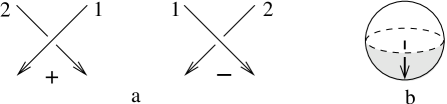
Figure 6. Signs of crossings and the south pole on $S^{2}$

Exercise 5.10.

There is a simple combinatorial way to compute $\operatorname{lk}(L_{1},L_{2})$ from any link diagram: count all crossings where $L_{1}$ passes over $L_{2}$, with signs shown in Figure 6a. Interpret this formula as a calculation of $\deg(\phi)$ by counting (with signs) the number of preimages of a certain regular value of $\phi$ (hint: look at Figure 6b). What formula would we get if we counted the preimages of the north pole?

For other graphs the situation is more complicated. For example, let $\Gamma=e$ be the graph with one edge, both ends of which end on the same link component, see Figure 5b. Then the configuration space $C_{e}$ is an open annulus $(R^{3})^{0}\times S^{1}\times\sigma^{1}\smallsetminus\Delta=S^{1}\times(0,1)$ (torus cut along the diagonal). The Gauss map $\phi$ is badly behaved near the diagonal, so the integrand blows up near the diagonal and we can not extend it to the closed torus. The integral nevertheless converges; one way to see it is to compactify $C_{e}$, cutting out of it some small neighborhood of the diagonal. This makes $C_{e}$ into a closed annulus $C^{\varepsilon}_{e}=S^{1}\times[\varepsilon,1-\varepsilon]$ (thus making the integral convergent) and we can recover the initial integral by taking $\varepsilon\to 0$. But the Gauss integral $W_{e}$ is no more a knot invariant: it may take any real value under a knot isotopy. A detailed discussion on this subject may be found in [5]. Why does this happen? The reason is that the compactified space $C_{e}$ is not a torus, but an annulus, so has a boundary and the degree of the Gauss map is not well-defined. When both ends of the edge start to collide together, the direction of the vector connecting them (which appears in the Gauss map) tends to the (positive or negative) tangent direction to the knot. The image of the unit tangent to the knot under the Gauss map is a certain curve $\gamma$ on $S^{2}$. One of the boundary circles $S^{1}\times\varepsilon$ and $S^{1}\times(1-\varepsilon)$ of $C^{\varepsilon}_{e}$ is mapped into $\gamma$, while the other is mapped into $-\gamma$, and the weight $W_{e}$ is part of the area of $S^{2}$ covered by the annulus $\phi(C^{\varepsilon}_{e})$ between these curves. Unfortunately, $\gamma$ may move on $S^{2}$ under an isotopy of $L$, so this area may change.

In this particular case there is a neat way to solve this problem: let $L$ be framed (i.e. fix a section of its normal bundle). We may think about the framing as about a unit normal vector $n(x)$ in each point $x$ of a knot. This allows us to slightly deform the Gauss map: $\phi_{(}x,y)\to\phi(x,y)+\varepsilon n(y)$. Now both boundary circles of the annulus $C_{e}$ map into the same curve on $S^{2}$ (why?) and we may glue the annulus into the torus so that the map $\phi_{\varepsilon}$ extends to it. It makes $W_{e}$ into an invariant of framed knots, called the self-linking number (the same result may be obtained by slightly pushing $L$ off itself along the framing and considering the linking number of the knot with its pushed-off copy).

It turns out that for other graphs there are also no divergence problems, so all integrals $W_{\Gamma}$ converge, and that a collision of all vertices of a graph to one point (so-called anomaly, see [18, 24]) is the only source of non-invariance, exactly as for $W_{e}$ above. Thus there is a suitable normalization of the expression (31) for $\langle L\rangle=\sum_{n}\langle L\rangle_{n}$ which gives a link invariant. To avoid a complicated explicit description of this normalization, let me formulate this result as follows:

Theorem 5.11 ([1], [18], [24]).

Let $L=\cup_{i=1}^{m}L_{i}$ be a link. Then $\langle L\rangle$ depends only on the isotopy class of $L$ and on the Gauss integrals $W_{e}(L_{i})$ of each component $L_{i}$. In particular, an evaluation of $\langle L\rangle$ at representatives of $L$ for which $W_{e}(L_{1})=\dots=W_{e}(L_{m})=0$ is a link invariant.

Remark 5.12.

It is known that this is a universal invariant of finite type. In particular this means that it is stronger than both the Alexander and the Jones polynomials (it contains the two-variable HOMFLY polynomial) and all other quantum invariants. Conjecturally the anomaly vanishes and this invariant coincides with the Kontsevich integral, see [18].

Example 5.13.

Let $L$ be a knot, and take $n=2$. There are four graphs of degree two, shown in Figure 5c. We will denote the first of them $X$, and the second by $Y$. By Exercise 5.7 the weight of the third graph vanishes. Also, choose a framing of $L$ so that the self-linking is 0; then the contribution of the last graph vanishes (another way to achieve the same result is to add to $\langle L\rangle_{2}$ a certain multiple of the self-linking number squared); we can set then $[X]=[Y]$. Thus we will consider simply

$$v_{2}=\frac{1}{4}\int_{C_{X}}\phi^{*}_{X}(\omega\wedge\omega)+\frac{1}{3}\int_{C_{Y}}\phi^{*}_{Y}(\omega\wedge\omega\wedge\omega).$$

The first integral is 4-dimensional, while the second is 6-dimensional; none of them separately is a knot invariant (see [20] for a discussion); however, their sum $v_{2}$ is (see [3], [20])! This invariant is, up to a constant, the second coefficient of the Alexander-Conway polynomial. See [20] for its detailed treatment as the degree of a Gauss-type map.

5.7. Degrees of maps

How can we explain the result of Theorem 5.11? We may try to repeat the reasoning of Example 5.8 in the general case. Recall that by Exercise 5.5 the dimensions of $C_{\Gamma}$ and $(S^{2})^{n}$ match, so if $C_{\Gamma}$ would be a closed manifold, then equation (32) would be a formula for a calculation of the degree of $\phi_{\Gamma}$. In other words, if $C_{\Gamma}$ would have a fundamental class, (32) would be its pairing with the pullback $\phi_{\Gamma}^{*}dvol$. That would be great: we would know that $W_{\Gamma}$ takes only integer values, and would be able to compute it in many ways, including a simple counting of preimages of any regular value of $\phi$.

Unfortunately, the reality is much worse: $C_{\Gamma}$ is an open space, so the degree is not well-defined and even the convergence is unclear. To guarantee the convergence, we should construct a compactification $\bar{C}_{\Gamma}$ of $C_{\Gamma}$ to which $\phi_{\Gamma}$ extends. This however will cause new problems: the space $\bar{C}_{\Gamma}$ will have many boundary strata. There are various way to deal with them: we can relativize some of them (i.e. consider a relative version of the theory), cap-off some others (i.e. glue to them some new auxiliary configuration spaces), or zip them up (gluing a stratum to itself by an involution). But in general, some boundary strata will remain; indeed, in Example 5.13 we have seen that none of $W_{X}$ or $W_{Y}$ separately can be made into a knot invariant. The remedy would be to glue together the configuration spaces for different graphs in $\widetilde{\mathfrak{J}}_{n}$ along the common boundary strata. This tedious work can be done indeed [18, 24] and (up to a certain anomaly correction) one can interpret $\langle L\rangle$ as the degree of a certain map $\Phi_{n}$ from a grand configuration space $\mathcal{C}_{n}$ to $(S^{2})^{n}$. Too many technicalities are involved to describe this construction in necessary details, so I refer the interested reader to [18, 24] and will present only a brief sketch of this construction.

The first problem is that initially the dimensions of $C_{\Gamma}$ for various $\Gamma\in\widetilde{\mathfrak{J}}_{n}$ do not match. E.g., in Example 5.13, for $n=2$ the spaces $C_{X}$ and $C_{Y}$ have dimensions 4 and 6 respectively. This can be fixed by considering a product $C_{\Gamma}\times(S^{2})^{k}$ of $C_{\Gamma}$ with enough spheres to make the maps $\phi_{\Gamma}\times(\text{id})^{k}$ to have the same target space $(S^{2})^{N}$ for all $\Gamma$. Now one should do the gluings. When two endpoints of an edge $e$ of a graph $\Gamma$ collide, the corresponding boundary stratum of $C_{\Gamma}$ looks like $C_{G}\times S^{2}$ for $G=\Gamma/e$. Thus we can glue together such strata for all pairs $(\Gamma,e)$ with isomorphic $G=\Gamma/e$. Some more, so-called hidden, strata remain after these main gluings. Fortunately, each of them can be zipped-up (i.e. glued to itself by a certain involution). The only codimension one boundary strata which remains after all these gluings are the anomaly strata, where all vertices of a graph $\Gamma\in\widetilde{\mathfrak{J}}$ collide together. These problematic anomaly strata can be glued [18] to a new auxiliary space. One ends up with a grand configuration space $\mathcal{C}_{n}$ endowed with a map $\Phi:\mathcal{C}_{n}\to(S^{2})^{N}$ (glued from the corresponding maps $\phi_{\Gamma}:\bar{C}_{\Gamma}\rightarrow(S^{2})^{N}$). One may show that the cohomology $H^{2N}(\mathcal{C}_{n})$ of this space projects surjectively to $\mathfrak{J}_{n}$ (see [17] for a similar case of 3-manifold invariants). Then $\langle L\rangle^{0}_{n}=\langle L\rangle_{n}+\text{anomaly correction}$ can be interpreted as the degree of $\Phi_{n}$, or more exactly, the image in $\mathfrak{J}_{n}$ of the fundamental class $[(S^{2})^{N}]$ under the induced composite map $\pi\circ\Phi^{*}:H^{2N}(S^{2})^{N}\to H^{2N}(\mathcal{C}_{n})\to\mathfrak{J}_{n}$.

5.8. Final remarks

There remain many questions: which compactification should we take, why do the antisymmetry and Jacobi relations appear in the cohomology of the grand configuration space, etc. Each of them is quite lengthy and is out of the scope of this note. We refer the interested reader to [5, 18, 24]. A mathematical treatment of invariants of 3-manifolds arising from the Chern-Simons theory was done in [2, 4]; I especially recommend [17]. While I do not know whether similar Feynman series arising in other topological problems always have a reformulation in terms of degrees of maps of some grand configuration space, it seems quite plausible. There are at least some other notable examples, see e.g. [19] for a similar interpretation of Kontsevich’s quantization of Poisson structures.

References

- [1] D. Altsch ler, L. Freidel, On universal Vassiliev invariants, Comm. Math. Phys. 170 (1995) 41–62.
- [2] S. Axelrod, I. M. Singer, Chern-Simons perturbation theory, Proc. XX DGM Conf. (New-York, 1991) (S. Catto and A. Rocha, eds.) World Scientific, 1992, 3–45; Chern-Simons perturbation theory II, J. Diff. Geom. 39 (1994) 173–213.
- [3] D. Bar-Nathan, Perturbative aspects of the Chern-Simons topological quantum field theory, Ph.D. thesis, Princeton Univ. 1991; Perturbative Chern-Simons theory, J. Knot Theory and Ramif. 4 (1995) 503–548.
- [4] R. Bott, A. Cattaneo, Integral invariants of -manifolds I, II, J. Diff. Geom. 48 (1998), 91–133, and J. Diff. Geom. 53 (1999), no. 1, 1–13.
- [5] R. Bott, C. Taubes, On the self-linking of knots, J. Math. Phys. 35 (1994) 5247–5287.
- [6] S. S. Chern, J. Simons, Some cohomology classes in principal fiber bundles and their application to riemannian geometry, Proc. Nat. Acad. Sci. U.S.A. 68 (1971) 791–794.
- [7] A. Connes, D. Kreimer, Renormalization in quantum field theory and the Riemann-Hilbert problem I, II, Commun.Math.Phys. 210 (2000) 249–273, Commun.Math.Phys. 216 (2001) 215–241.
- [8] E. T. Copson, Asymptotic expansions, Cambridge Tracts in Math. and Math. Phys. 55, 1967.
- [9] Quantum fields and strings: a course for mathematicians, vol 1-2, (P. Deligne et al, eds.) AMS 1999.
- [10] A. Dubrovin, A. Fomenko, S. Novikov, Modern geometry— methods and applications. Part II. The geometry and topology of manifolds, Graduate Texts in Mathematics, 104, Springer, 1985.
- [11] D. Freed, Classical Chern-Simons theory I, II, Adv. Math. 113 (1995) 237–303, Houston J. Math. 28 (2002) 293–310.
- [12] J.-M. Drouffe, C. Itzykson, Statistical field theory, Cambridge Univ.Press, 1989.
- [13] L. D. Faddeev, V. N. Slavnov, Gauge fields, introduction to quantum theory, Benjamin/Cummings, Reading, 1980.
- [14] W. Fulton, R. D. MacPherson, A compactification of configuration spaces., Annals of Math. (2) 139 (1994), 183–225.
- [15] E. Guadagnini, M. Martinelli, M. Mintchev, Perturbative aspects of the Chern-Simons field theory, Phys. Let. B277 (1989) 111; Chern-Simons field theory and link invariants, Nucl. Phys. B330 (1990) 575–607.
- [16] C. Itzykson, J. Zuber, Quantum field theory, McGraw-Hill, New-York, 1985.
- [17] G. Kuperberg, D. Thurston, Perturbative 3-manifold invariants by cut-and-paste topology, math.GT/9912167.
- [18] S. Poirier, The Configuration space integral for links in , Algebr. Geom. Topol. 2 (2002) 1001–1050.
- [19] M. Polyak, Quantization of linear Poisson structures and degrees of maps, Let. Math. Phys. 60 (2003) 15–35.
- [20] M. Polyak, O. Viro, On the Casson knot invariant, J. Knot Theory and Ramif. 10 (2001) 711–738.
- [21] A. Polyakov, Gauge fields and strings, Harwood academic publishers, 1987.
- [22] S. Schweber, An introduction to relativistic quantum field theory, Row, Peterson 1961.
- [23] A. S. Schwarz, Quantum field theory and topology, Springer, 1993.
- [24] D. Thurston, Integral expressions for the Vassiliev knot invariants, M.A. thesis, Harvard Univ. 1995, math.QA/9901110.
- [25] E. Witten, Quantum field theory and the Jones polynomial, Comm. Math. Phys. 121 (1989) 351–399.