Fibonomial Cumulative Connection Constants

Abstract

In this note we present examples of cumulative connection constants - new Fibonomial ones included. All examples posses combinatorial interpretation.

This presentation is an update of A.K.Kwaśniewski Fibonomial cumulative connection constants Bulletin of the ICA vol. 44 (2005), 81-92.

AMS Classification Numbers: 06A06 ,05B20, 05C75, 05A40

this electronic paper is affiliated to The Internet Gian-Carlo Polish Seminar:

http://ii.uwb.edu.pl/akk/sem/sem_rota.htm

1 Introduction

The cumulative connection constants (ccc) $C_{n}$ were introduced by the Authors of [1]:

$$C_{n}=\sum_{k\geq 0}c_{n,k}\;,\;\;\;n\geq 0,$$

where

$$p_{n}(x)=\sum_{0\leq k\leq n}c_{n,k}q_{k}(x)$$

and Pascal-like array $\left\{c_{n,k}\right\}_{n,k\geq 0}$ of connection constants $c_{n,k},\;\;n,k\geq 0$ ”connects” two polynomial sequences (Note: $\left\{p_{k}(x)\right\}_{k\geq 0}$ is a polynomial sequence if $\deg p_{k}=k$).

Motivation 1
”The connection constants problem” i.e. combinatorial interpretations, algorithms of calculation , recurrences and other properties - is one of the central issues of the binomial enumeration in Finite Operator Calculus (FOC ) of Rota-Roman and Others and in its afterwards extensions (see: abundant references in [8]-[10],[13]). Important knowledge on recurrences for $\left\{c_{n,k}\right\}_{n,k\geq 0}$ one draws from [2] - consult also the NAVIMA group program:
http://webs.uvigo.es/t10/navima/ .

Motivation 2
The cumulative connection constants (ccc) as defined above appear to represent combinatorial quantities of primary importance - as shown by examples below .

A special case of interest considered in [2, 1] is the case of monic persistent root polynomial sequences [3] characterized by the following conditions:

$$p_{0}(x)=q_{0}(x)=1\;;\;\;q_{n}(x)=q_{n-1}(x)(x-r_{n})\;,\;p_{n}(x)=p_{n-1}(x)(x-s_{n})\;\;\;\;n\geq 1.$$

The pair of persistent root polynomial sequences and hence corresponding connection constants array are then bijectively labeled by the pair of root sequences :

$$[r]=\left\{r_{k}\right\}_{k\geq 1},\;\;\;[s]=\left\{s_{k}\right\}_{k\geq 1}.$$

In this particular case of persistent root polynomial sequences the authors of [2] gave a particular name to connection constants : ”generalized Lah numbers” - now denoted as follows $c_{n,k}=L_{n,k}$. The generalized Lah numbers do satisfy the following recurrence [2, 1] :

$$L_{n+1,k}=L_{n,k-1}+(r_{k+1}-s_{n+1})L_{n,k}$$ (1)

$$L_{0,0}=1\;,\;\;L_{0,-1}=0\;\;\;n,k\geq 0$$

from which the recurrence for cumulative connection constants (ccc) follows

$$C_{n+1}=(1-s_{n+1})C_{n}+\sum_{k=0}^{n}c_{n,k}r_{k+1}$$ (2)

where $c_{n,k}=L_{n,k}$.

The clue examples of [1] are given by the following choice of a pair of root sequences :
the Fibonacci sequence

$C_{n}=F_{n};\;\;n>0\;\longleftrightarrow[r]=\left\{r_{k}\right\}_{k\geq 1}=\left\{0,0,0,0,0,0,\ldots\right\},\;[s]=\left\{s_{k}\right\}_{k\geq 1}=\left\{0,0,...,0,...\right\}=[0]$

the Lucas sequence

$C_{n}=L_{n}\;;\;n>0\longleftrightarrow[r]=\left\{r_{k}\right\}_{k\geq 1};\;\;r_{1}=0,r_{2}=2,r_{k}=1-(r_{k-1})^{2}$ for $k>2$ and $[s]=[0]$.

2 Examples of cumulative connection constants - old and new

We shall supply now several examples of connection constants arrays and corresponding ccc‘s - Fibonomial case included - altogether with their combinatorial interpretation. (HELP! - For notation-help - see: Appendix ).

Example 1. $c_{n,k}=\binom{n}{k},\;\;x^{n}=\sum_{k\geq 0}\binom{n}{n}(x-1)^{k}\;\;\;n\geq 0;\\ E^{-1}(D)x^{k}=(x-1)^{k}\;\;n\geq 0.$

$$C_{n}=\sum_{k\geq 0}\binom{n}{k}=2^{n}=number\;\;of\;all\;subsets\;of\;S;\;\;n=|S|;n\geq 0.$$

Here $E^{a}(D)=\sum_{n\geq 0}\frac{a^{n}}{n!}D^{n}$ is the translation operator ($D=\frac{d}{dx}$ ) and the recurrence (2) is obvious.

Example 2. $c_{n,k}=\Big{\{}{n\atop k}\Big{\}}$ denote Stirling numbers of the second type. Then $x^{n}=\sum_{k=0}^{n}\Big{\{}{n\atop k}\Big{\}}x^{\underline{k}}$ . Let $B_{n}=\sum_{k=0}^{n}\Big{\{}{n\atop k}\Big{\}}$ , then
$B_{n}=number\;of\;all\;partitions\;of\;S;\;n=|S|$;$B_{n}\equiv$ Bell numbers.

As the recurrence for Bell numbers reads $B_{n+1}=\sum_{k=0}^{n}\binom{n}{k}B_{k}\;;\;\;n\geq 0$ we easily get from (2) the inspiring identity

$$\sum_{k=0}^{n}\binom{n}{k}B_{k}=B_{n}+\sum_{k=1}^{n}\Big{\{}{n\atop k}\Big{\}}k.$$

Example 3. $c_{n,k}=\Big{[}{n\atop k}\Big{]}$ are Stirling numbers of the first kind . Then $x^{\overline{n}}=\sum_{k=0}^{n}\Big{[}{n\atop k}\Big{]}x^{k},\;n\geq 0$. $C_{n}=\sum_{k=0}^{n}\Big{[}{n\atop k}\Big{]}=n!$ and the obvious recurrence $C_{n+1}=(n+1)C_{n}$ coincides with (2) .

Example 4. $c_{n,k}=\binom{n}{k}_{q},\;x^{n}=\sum_{k\geq 0}\binom{n}{k}_{q}\Phi_{k}(x),\;\;\;\Phi_{k}(x)=\prod_{s=0}^{k-1}(x-q^{s})$,

$$C_{n}=\sum_{k\geq 0}\binom{n}{k}_{q}=number\;\;of\;\;all\;\;subspaces\;\;of\;\;V(n,q)\;\;i.e.$$

$$C_{n}=\sum_{k=0}^{n}\binom{n}{k}_{q}=\left|L(n,q)\right|\equiv(1+_{q}1)^{n},$$

where $L(n,q)$ denotes the lattice of all subspaces of $V(n,q)$ - ( the $n$-th dimensional space $V(n,q)$ over Galois field $GF(q)$ ) - see: [4] .
According to Konvalina

$$C_{n}=\sum_{k=0}^{n}\binom{n}{k}_{q}\equiv(1+_{q}1)^{n}$$

is at the same time the number of all possible choices with repetition of objects from exponentially weighted boxes [5, 6].
As $q$-Gaussian polynomials $\Phi_{k}(x)=\prod_{s=0}^{k-1}(x-q^{s})$ constitute a persistent root polynomial sequence - the generalized Lah numbers - which are now are $\binom{n}{k}_{q}=c_{n,k}=L_{n,k}$ must satisfy the recurrence equation

$$L_{n+1,k}=L_{n,k-1}+r_{k+1}L_{n,k},\;\;L_{0,0}=1,\;\;L_{0,-1}=0\;\;\;n,k\geq 0,$$

where $[r]=\left\{q^{k-1}\right\}_{k\geq 1}$ is the root sequence determining $\left\{\Phi_{n}\right\}_{n\geq 0}$. See Appendix 2. Hence the recurrence (2) for the number $C_{n}$ of all possible choices with repetition of objects from exponentially weighted boxes [5, 6] is of the form

$$C_{n+1}=C_{n}+\sum_{k=0}^{n}\binom{n}{k}_{q}q^{k}$$

because

$$C_{n+1}=C_{n}+\sum_{k=0}^{n}c_{n,k}r_{k+1}.$$

In another $q$-umbral notation (see: Appendix 2)

$$(1+_{q}1)^{n+1}=(1+_{q}1)^{n}+\sum_{k=0}^{n}\binom{n}{k}_{q}q^{k}.$$

Occasionally note that using the Möbius inversion formula (see: [4] - the $q$-binomial theorem Corollaries in section 5 - included ) we have

$$x^{n}=\sum_{k\geq 0}\binom{n}{k}_{q}\Phi_{k}(x),\;\;\;\;\Phi_{k}(x)=\sum_{l\geq 0}\binom{k}{l}_{q}(-1)^{l}q^{\binom{l}{2}}x^{k-l},\;\;n\geq 0$$

i.e. the identity

$$\prod_{s=0}^{k-1}(x-q^{s})\equiv\sum_{l\geq 0}\binom{k}{l}_{q}(_{1})^{l}q^{\binom{l}{2}}x^{k-l}.$$

”The Möbius $q$-inverse example” is then the following.

Example 4’. $c_{n,k}=\binom{n}{k}_{q}(-1)^{n-k}q^{\binom{n-k}{2}},\;\;x^{n}=\sum_{k\geq 0}c_{n,k}H_{k}(x)$, where (written with help of generalized shift operator [7, 8, 9, 10] - analogously to the use of $E^{-1}(D)x^{k}=(x-1)^{k}$ above in Example 1. ) we have (see Appendix 2):

$$H_{k}(x)=E(\partial_{q})x^{k}\equiv(x+_{q}1)^{k}=\sum_{l\geq 0}\binom{k}{l}_{q}x^{l}.$$

Compare with $H_{k}(x,y)|_{y=1}=H_{k}(x)$ in [11] (pp. 240-241) and note that

$$C_{n}=\sum_{k=0}^{n}|c_{n,k}|=\sum_{k=0}^{n}\binom{n}{k}_{q}q^{\binom{k}{2}}$$

is the number of all possible choices without repetition of objects from exponentially weighted boxes [5, 6]. It is then combinatorial - natural to consider also another triad .

Example 4”. $c_{n,k}=\binom{n}{k}_{q}q^{\binom{k}{2}},\;\;x^{n}=\sum_{k\geq 0}\binom{n}{k}_{q}q^{\binom{n}{2}}\Gamma_{k}(x),\\ \Gamma_{k}(x)=\sum_{l\geq 0}\binom{k}{l}_{q}(-1)^{k-l}x^{l},\;\;n\geq 0$.

Example 5. This is The Fibonomial Example: $c_{n,k}=\binom{n}{k}_{F},\\ x^{n}=\sum_{k\geq 0}\binom{n}{k}_{F}\Xi_{k}(x)$ where $\binom{n}{k}_{F}$ are called Fibonomial coefficients (see A3). Using the Möbius inversion formula - analogously to the Example 4 case - we get

$$\Xi_{k}(x)=\sum_{l\geq 0}\binom{k}{l}_{f}\mu(l,k)x^{k-1},\;\;n\geq 0,$$

where Möbius matrix $\mu$ is the unique inverse of the incidence matrix $\zeta$ defined for the ”Fibonacci cobweb” poset introduced in [12] (see: A4 for explicit formula of $\zeta$ from [16] ). For combinatorial interpretation of these Fibonomial coefficients see: Appendix 4. Interpretation of $C_{n}$ stated below results from combinatorial interpretation of Fibonomial coefficients. Combinatorial interpretation of ccc $C_{n}$ in this case is then the following:

$C_{n}=\sum_{k\geq 0}\binom{n}{k_{F}}=$number of all such subposets of the Fibonacci cobweb poset $P$ which are cobweb subposets starting from the level $F_{k}$ and ending at the level labeled by $F_{n}$.

As in the $q$-umbral case of the Example 4 we have ”$F$-umbral” representation of the Fibonomial ccc $C_{n}$ ( see A3) . Namely

$$C_{n}=\sum_{k=0}^{n}\binom{n}{k}_{F}\equiv(1+_{F}1)^{n}$$

3 Remark on ccc - recurrences ”exercise”

ccc-recurrences from examples 1-4 were an easy game to play. All these four cases of ccc might be interpreted on equal footing due to the ingenious scheme of one unified combinatorial interpretation by Konvalina [5, 6].

As for the other cases the ”exercise” of finding the recurrences for ccc - up to the Fibonomial case - might be the slightly harder task. In this last case with Fibonomial coefficients one may derive the well known recurrence

$$\binom{n+1}{k}_{F}=F_{k-1}\binom{n}{k}_{F}+F_{n-k+2}\binom{n}{k-1}_{F}$$ (3)

$$\binom{n}{0}_{F}=1,\;\;\binom{0}{k}_{F}=0\;\;\mathrm{for}\;\;k>0$$

or equivalently

$$\binom{n+1}{k}_{F}=F_{k+1}\binom{n}{k}_{F}+F_{n-k}\binom{n}{k-1}_{F}$$

$$\binom{n}{0}_{F}=1,\;\;\binom{0}{k}_{F}=0\;\;\mathrm{for}\;\;k>0$$

also by combinatorial reasoning [16] (it might be a hard exercise - not to check it but to prove it another way - a use of [2] - being recommended). Derivation of the recurrence for Fibonomial ccc $C_{n}$ - we leave as an exercise.

4 Appendix

4.1 On the notation used trough out in this note

$q$-binomial and Fibonomial cases are specifications of the $\psi$-sequence choice in the so called $\psi$- calculus notation [8]-[10] in conformity with [14] referring back to works of Brenke and Boas on generalized Appell polynomials (see abundant references in [9])

4.2 $q$-Gaussian ccc

$$\binom{n+1}{k}_{q}=q^{k}\binom{n}{k}_{q}+\binom{n}{k-1}_{q}$$ (4)

$$\binom{n}{0}_{q}=1,\;\;n\geq 0,k\geq 1,$$

where $n_{q}!=n_{q}(n-1)_{q}!;\;\;1_{q}!=)_{q}!=1,\;\;n_{q}^{\underline{k}}=n_{q}(n-1)_{q}\ldots(n-k+1)_{q},\\ \binom{n}{k}_{q}\equiv\frac{n_{q}^{\underline{k}}}{k_{q}!}$.

Remark 4.1.

(see [15]) The dual to (4) reccurrenceis then given by

$$x\Phi_{n}(x)=q^{n}\Phi_{n}(x)+\Phi_{n+1}(x)$$ (5)

$$\Phi_{0}(x)=1,\;\;\Phi_{-1}(x)=0;\;\;n\geq 0,$$

in accordance with a well known fact (see: [4] ) that

$$x^{n}=\sum_{k\geq 0}\binom{n}{k}_{q}\Phi_{k}(x),$$ (6)

where $\Phi_{k}(x)=\prod_{s=0}^{k-1}(x-q^{s})$ are the $q$-Gaussian polynomials.

Recall now that the Jackson $\partial_{q}$- derivative is defined as follows [7]-[11]: $\left(\partial_{q}\varphi\right)(x)=\frac{\varphi(x)-\varphi(qx)}{(1-q)x}$ - and is also called the $q$-derivative. The consequent notation for the generalized shift operator [7]-[10],[13] is:

$$E^{a}(\partial_{q})x^{n}=\exp_{q}\{a\partial_{q}\}=\sum_{k=0}^{\infty}\frac{a^{k}}{k_{q}!}\partial_{q}^{k}.$$

Then we identify $E^{y}(\partial_{q})x^{n}\equiv(x+_{q}y)^{n}$. (Ward in [7] does not use any subscript like $q$ or $F$ or $\psi$.

Naturally his $"+"$ means not $+$ but a ”plus with a subscript” in our notation).

4.3 Fibonomial notation

In straightforward analogy consider now the Fibonomial coefficients $c_{n,k}$,

$$c_{n,k}=\binom{n}{k}_{F}=\frac{F_{n}!}{F_{k}!F_{n-k}!}=\binom{n}{n-k}_{F},$$

where $n_{F}\equiv F_{n}$,$n_{F}!\equiv n_{F}(n-1)_{F}(n-2)_{F}(n-3)_{F}\ldots 2_{F}1_{F};\;\;0_{F}!=1$;$n_{F}^{\underline{k}}=n_{F}(n-1)_{F}\ldots(n-k+1)_{F};\;\;\;\binom{n}{k}_{F}\equiv\frac{n^{\underline{k}}_{F}}{k_{F}!}$ and linear difference operator $\partial_{F}$ acting as follows: $\partial_{F};\;\;\partial_{F}x^{n}=n_{F}x^{n-1};\;\;n\geq 0$ - we shall call the $F$-derivative. Then in conformity with [7] and with notation as in [10, 9, 8, 13] one writes:

1. $\left(x+_{F}a\right)^{n}\equiv\sum_{k\geq 0}\binom{n}{k}_{F}a^{k}x^{n-k}$ where $\binom{n}{k}_{F}\equiv\frac{n^{\underline{k}}_{F}}{k_{F}!}$
   and $n_{F}^{\underline{k}}=n_{F}(n-1)_{F}\ldots(n-k+1)_{F}$;

2. $\left(x+_{F}a\right)^{n}\equiv E^{a}(\partial_{F}x^{n};\;\;E^{a}(\partial_{F})=\sum_{n\geq 0}\frac{a^{n}}{n_{F}!}\partial_{F}^{n};\;\;\\ E^{a}(\partial_{F})f(x)=f(x+_{F}a),$ $E^{a}(\partial_{F})$ is corresponding generalized translation operator.

4.4 Combinatorial interpretation of Fibonomial Coefficients [12, 16, 17, 18, 19, 20]

Let us depict a partially ordered infinite set $P$ via its finite part Hasse diagram to be continued ad infinitum in an obvious way as seen from the figure below.

This Fibonacci cobweb partially ordered infinite set $P$ is defined as in [12] via its finite part - cobweb subposet $P_{m}$(rooted at $F_{1}$ level subposet) to be continued ad infinitum in an obvious way as seen from the figure of $P_{5}$ below. It looks like the Fibonacci tree with a specific ”cobweb”. It is identified with Hasse diagram of the partial order set $P$ .

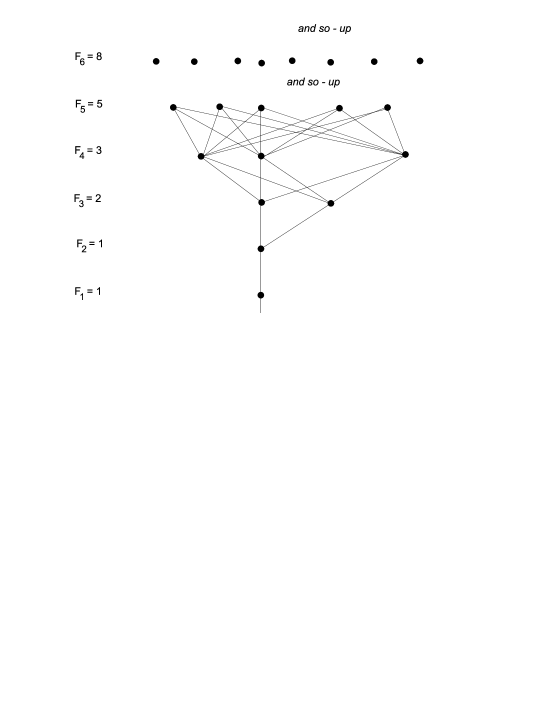
Figure 1: The graded structure of the Fibonacci cobweb poset

If one defines this poset $P$ with help of its incidence matrix $\zeta$ representing $P$ uniquely then one arrives at $\zeta$ with easily recognizable staircase-like structure - of zeros in the upper part of this upper triangle matrix $\zeta$. This structure is depicted by the Figure 2 where: empty places mean zero values (under diagonal) and in filled with - -…- parts of rows (above the diagonal) ”‘-”’ stay for ones. The picture below is drawn for the sequence $F=\left\langle F_{\textbf{ {\color[rgb]{1,0,0}1}}},F_{2},F_{3},...,F_{n},...\right\rangle$, where $F_{k}$ are Fibonacci numbers.

1 - - - - - - - - - - - - - - - - - - - - - - - - - - - - - - - - - - - - - - - - - - - - - - - - - - -

1 - - - - - - - - - - - - - - - - - - - - - - - - - - - - - - - - - - - - - - - - - - - - - - - -

1 0 - - - - - - - - - - - - - - - - - - - - - - - - - - - - - - - - - - - - - - - - - - - - - -

1 - - - - - - - - - - - - - - - - - - - - - - - - - - - - - - - - - - - - - - - - - - - - - - -

1 0 0 - - - - - - - - - - - - - - - - - - - - - - - - - - - - - - - - - - - - - - - - - - -

1 0 - - - - - - - - - - - - - - - - - - - - - - - - - - - - - - - - - - - - - - - - - - -

1 - - - - - - - - - - - - - - - - - - - - - - - - - - - - - - - - - - - - - - - - - - -

$F_{5}-1\;\textbf{{\color[rgb]{1,0,0}0}}^{\prime}s\;\;$1 0 0 0 0 - - - - - - - - - - - - - - - - - - - - - - - - - - - - - - - - - - - -

1 0 0 0 - - - - - - - - - - - - - - - - - - - - - - - - - - - - - - - - - - - -

1 0 0 - - - - - - - - - - - - - - - - - - - - - - - - - - - - - - - - - - - -

1 0 - - - - - - - - - - - - - - - - - - - - - - - - - - - - - - - - - - - -

1 - - - - - - - - - - - - - - - - - - - - - - - - - - - - - - - - - - - -

$F_{6}-1\;zeros\quad\quad\quad\quad$1 0 0 0 0 0 0 0 - - - - - - - - - - - - - - - - - - - - - - - - - -

1 0 0 0 0 0 0 - - - - - - - - - - - - - - - - - - - - - - - - -

1 0 0 0 0 0 - - - - - - - - - - - - - - - - - - - - - - - - -

1 0 0 0 0 - - - - - - - - - - - - - - - - - - - - - - - - -

1 0 0 0 - - - - - - - - - - - - - - - - - - - - - - - - -

1 0 0 - - - - - - - - - - - - - - - - - - - - - - - - -

1 0 - - - - - - - - - - - - - - - - - - - - - - - - -

1 - - - - - - - - - - - - - - - - - - - - - - - - -

$F_{7}-1\;zeros\quad\quad\quad\quad\quad\quad\quad\quad\quad\quad\;$1 0 0 0 0 0 0 0 0 0 0 0 0 - - - - - - -

1 0 0 0 0 0 0 0 0 0 0 0 - - - - - - -

1 0 0 0 0 0 0 0 0 0 0 - - - - - - -

1 0 0 0 0 0 0 0 0 0 - - - - - - -

1 0 0 0 0 0 0 0 0 - - - - - - -

1 0 0 0 0 0 0 0 - - - - - - -

1 0 0 0 0 0 0 - - - - - - -

1 0 0 0 0 0 - - - - - - -

1 0 0 0 0 - - - - - - -

1 0 0 0 - - - - - - -

1 0 0 - - - - - - -

1 0 - - - - - - -

1 - - - - - - -

$F_{8}-1\;zeros\quad\quad\quad\quad\quad\quad\quad\quad\quad\quad\quad\quad\quad\quad\quad\quad\quad\quad\quad\quad\;\,$…………………….

and so on

Fig. La Scala di Fibonacci. The staircase structure of incidence matrix $\zeta\in I(P,R)$ = incidence algebra of $P$ over the commutative ring $R$. See [12](2003)

For many pictures and further progress on cobweb posets and KoDAGs consult [17-29,31-42].

The characteristic function $\chi_{F}(\leq)$ = $\zeta_{F}(\leq)$ of the partial order relation $\leq$ of the graded $F$-cobweb poset $P$ - or in brief just $\zeta$ - might be expressed by Kronecker delta as here down ([18] (2003) and see also [12,40,18,16]) for any natural numbers valued sequence $F$ - including the motivating example with Fibonacci sequence $F$ denominated graded cobweb poset $P$ for which it reads ($F_{0}=\textbf{{\color[rgb]{1,0,0}0}}$):

Kwaśniewski $\zeta$ 2003 formula

$$\zeta=\zeta_{1}-\zeta_{0}$$

where for $x,y\in{\bf N}$:

$$\zeta_{1}(x,y)=\sum_{k=0}^{\infty}\delta(x+k,y)$$

$$\zeta_{0}(x,y)=\sum_{k\geq 0}\sum_{s\geq 0}\delta(x,F_{s+1}+k)\sum_{r=1}^{F_{s}-k-1}\delta(k+F_{s+1}+r,y)$$

and naturally

$$\delta(x,y)=\Big{\{}\begin{array}[]{l}1\;\;\;\;\;x=y\\ 0\;\;\;\;\;x\neq y\end{array}.$$

Right from the Hasse diagram of $P$ here now obvious observations follow.

Observation 4.1.

The number of maximal chains starting from the root (level $F_{1}$ ) to reach any point at the $n$-th level labeled by $F_{n}$ is equal to $n_{F}!$.

Observation 4.2.

The number of maximal chains starting from any fixed point at the level labeled by $F_{k}$ to reach any point at the $n$-th level labeled by $F_{n}$ is equal to $n^{\underline{m}}_{F}\;\;(n=k+m)$ .

Let us denote by $P_{m}$ a subposet of $P$ with vertices up to $m$-th level vertices

$$\bigcup_{s=1}^{m}\Phi_{s}\;\;;\;\Phi_{s}\;\;is\;\;the\;\;set\;\;of\;\;elements\;\;of\;\;the\;\;s-th\;\;level$$

.

Attention please. $P_{m}$ depending on the context is also to be viewed on as representing the set of maximal chains. It is naturally a particular case of the layer of graded poset called cobweb poset [1-23] - for the reader convenience - see Appendix with basic ponderables. For the sake of coming right now combinatorial interpretation, all layers on one hand are viewed on as subposets while on the other hand are also to be viewed on as representing the set of maximal chains.

Consider now the following behavior of a ”sub-cob” moving from any given point of the $F_{k}$ level of the poset up. It behaves as it has been born right there and can reach at first $F_{2}$ points up then $F_{3}$ points up , $F_{4}$ and so on - thus climbing up to the level $F_{k+m}=F_{n}$ of the poset $P$. It can see - as its Great Ancestor at the root $F_{1}$-th level and potentially follow one of its own accessible finite subposet $P_{m}$. One of many $P_{m}$ ‘s rooted at the $k$-th level might be found. How many?

The answer for the Fibonacci sequence $F$ was given in [12] (2003) :

Observation 4.3.

Let $n=k+m$. The number of subposets equipotent to subposet $P_{m}$ rooted at any fixed point at the level labeled by $F_{k}$ and ending at the $n$-th level labeled by $F_{n}$ is equal to

$$\binom{n}{m}_{F}=\binom{n}{k}_{F}=\frac{n^{\underline{k}}_{F}}{k_{F}!}.$$

Equivalently - now in a bit more mature 2009 year the answer is given simultaneously viewing layers as biunivoquely representing maximal chains sets. Let us make it formal.

Such recent equivalent formulation of this combinatorial interpretation is to be found in [20] from where we quote it here down.

Let $\left\{F_{n}\right\}_{n\geq 0}$ be a natural numbers valued sequence with $F_{0}=1$ (or $F_{0}!\equiv 0!$ being exceptional as in case of Fibonacci numbers). Any such sequence uniquely designates both $F$-nomial coefficients of an $F$-extended umbral calculus as well as $F$-cobweb poset introduced by this author (see :the source [19] from 2005 and earlier references therein). If these $F$-nomial coefficients are natural numbers or zero then we call the sequence $F$ - the $F$-cobweb admissible sequence.

Definition 4.1.

Let any $F$-cobweb admissible sequence be given then $F$-nomial coefficients are defined as follows

$${{n}\choose{k}}_{F}=\frac{n_{F}!}{k_{F}!(n-k)_{F}!}=\frac{n_{F}\cdot(n-1)_{F}\cdot...\cdot(n-k+1)_{F}}{1_{F}\cdot 2_{F}\cdot...\cdot k_{F}}=\frac{n^{\underline{k}}_{F}}{k_{F}!}$$

while $n,k\in N$ and $0_{F}!=n^{\underline{0}}_{F}=1$.

Definition 4.2.

$C_{max}(P_{n})\equiv\left\{c=<x_{0},x_{1},...,x_{n}>,\>x_{s}\in\Phi_{s},\>s=0,...,n\right\}$ i.e. $C_{max}(P_{n})$ is the set of all maximal chains of $P_{n}$

Definition 4.3.

Let

$$C_{max}\langle\Phi_{k}\to\Phi_{n}\rangle\equiv\left\{c=<x_{k},x_{k+1},...,x_{n}>,\>x_{s}\in\Phi_{s},\>s=k,...,n\right\}.$$

Then the $C\langle\Phi_{k}\to\Phi_{n}\rangle$ set of Hasse sub-diagram corresponding maximal chains defines biunivoquely the layer $\langle\Phi_{k}\to\Phi_{n}\rangle=\bigcup_{s=k}^{n}\Phi_{s}$ as the set of maximal chains’ nodes and vice versa - for these graded DAGs (KoDAGs included).

The equivalent to that of of Obsevation 3 formulation of combinatorial interpretation of cobweb posets via their cover relation digraphs (Hasse diagrams) is the following.

Theorem [20]
(Kwaśniewski) For $F$-cobweb admissible sequences $F$-nomial coefficient ${{n}\choose{k}}_{F}$ is the cardinality of the family of equipotent to $C_{max}(P_{m})$ mutually disjoint maximal chains sets, all together partitioning the set of maximal chains $C_{max}\langle\Phi_{k+1}\to\Phi_{n}\rangle$ of the layer $\langle\Phi_{k+1}\to\Phi_{n}\rangle$, where $m=n-k$.

For February 2009 readings on further progress in combinatorial interpretation and application of the presented author invention i.e. partial order posets named cobweb posets and their’s corresponding encoding Hasse diagrams KoDAGs see [19-29,31-42] and references therein. For active presentation of cobweb posets see [40]. This electronic paper is an update of [41]

5 Summarizing , Concluding ad upgrade and ad references remarks

Remark 1 The matrix elements of $\zeta(x,y)$ were given in 2003 ([18] Kwaśniewski) using $x,y\in N\cup\left\{0\right\}$ labels of vertices in their ”‘natural”’ linear order:
1. set $k=0$,
2. then label subsequent vertices - from the left to the right - along the level $k$,
3. repeat 2. for $k\rightarrow k+1$ until $k=n+1$ ; $n\in N\cup\left\{\infty\right\}$

As the result we obtain the $\zeta$ matrix for Fibonacci sequence as presented by the the Fig. La Scala di Fibonacci dating back to 2003 [18,41].

Inspired [8,9,13] by Gauss $n_{q}=q^{0}+q^{1}+...+q^{n-1}$ finite geometries numbers and in the spirit of Knuth ”‘notationlogy”’ [30] we shall refer here also to the upside down notation effectiveness as in [21-24,20] or earlier in [8,9,10,13], (consult also the Appendix in [33]). As for that upside down attitude $F_{n}\equiv n_{F}$ being much more than ”‘just a convention”’ to be used substantially in what follows as well as for the sake of completeness - let us quote it as The Principle according to Kwasśniewski [42] where it has been formulated as an ”‘of course”’ Principle i.e. simultaneously trivial and powerful statement.

The Upside Down Notation Principle.
1. Let the statement $s(F)$ depends only on the fact that $F$ is a natural numbers valued statement.
2. Then if one proves that $s(N)\equiv s(\left\langle n\right\rangle_{n\in N})$ is true - the statement $s(F)\equiv s(\left\langle n_{F}\right\rangle_{n\in N})$ is also true. Formally - use equivalence relation classes induced by co-images of $s:\left\{F\right\}\mapsto 2^{\left\{1\right\}}$ and proceed in a standard way.

In order to proceed further let us now recall-rewrite purposely here Kwaśniewski $2003$ - formula for $\zeta$ function of arbitrary cobweb poset so as to see that its’ algorithm rules authomatically make it valid for all $F$-cobweb posets where $F$ is any natural numbers valued sequence i.e. with $F_{0}>0$. $I(\Pi,R)$ stays for the incidence algebra of the poset $\Pi$ over the commutative ring $R$.

$$\zeta(x,y)=\zeta_{1}(x,y)-\zeta_{0}(x,y)$$

$$\zeta_{{\color[rgb]{0,1,0}\textbf{1}}}(x,y)=\sum_{k={\color[rgb]{0,0,1}\textbf{0}}}^{\infty}\delta(x+k,y)$$

$$\zeta_{0}(x,y)=\sum_{k\geq{\color[rgb]{1,0,0}\textbf{1}}}\sum_{s\geq 0}\delta(x,F_{s+1}+k)\sum_{r=1}^{F_{s}-k-1}\delta(k+F_{s+1}+r,y)$$

and naturally

$$\delta(x,y)=\Big{\{}\begin{array}[]{l}1\;\;\;\;\;x=y\\ 0\;\;\;\;\;x\neq y\end{array}.$$

The above formula for $\zeta\in I(\Pi,R)$ rewritten in ($F_{s}\equiv s_{F}$) upside down notation equivalent form as below is of course valid for all cobweb posets.

$$\zeta(x,y)=\zeta_{{\color[rgb]{0,1,0}\textbf{{\color[rgb]{0,1,0}{1}}}}}(x,y)-\zeta_{0}(x,y),$$

$$\zeta_{{\color[rgb]{0,1,0}\textbf{1}}}(x,y)=\sum_{k={\color[rgb]{0,0,1}\textbf{0}}}^{\infty}\delta(x+k,y),$$

$$\zeta_{0}(x,y)=\sum_{s\geq 1}\sum_{k\geq{\color[rgb]{1,0,0}\textbf{1}}}\delta(x,k+s_{F})\sum_{r=1}^{(s-1)_{F}-k-1}\delta(x+r,y).$$

Note. $+\zeta_{{\color[rgb]{0,1,0}\textbf{1}}}$ ”‘produces the Pacific ocean of 1’s”’ in the whole upper triangle part of a would be incidence algebra $\sigma\in I(\Pi,R)$ matrix elements

Note. $-\zeta_{0}$ cuts out 0’s i.e. thus producing ”‘zeros’ $F$-La Scala staircase”’ in the 1’s delivered by $+\zeta_{{\color[rgb]{0,1,0}\textbf{1}}}$.

This results exactly in forming 0’s rectangular triangles: $s_{F}-1$ of them at the start of subsequent stair and then down to one 0 till - after $s_{F}-1$ rows passed by one reaches a half-line of $1^{\prime}s$ which is running to the right- right to infinity and thus marks the next in order stair of the $F$- La Scala.

The $\zeta$ matrix explicit formula was given for arbitrary graded posets with the finite set of minimal in terms of natural join of bipartite digraphs in SNACK = the Sylvester Night Article on KoDAGs and Cobwebs = [21].

What was said is equivalent to the fact that the cobweb poset coding La Scala is of the natural join operation origin while thus producing $\zeta$ matrix [23,21,24] which is of the form (quote from SNACK = [21], see: Subsection 2.6.)

The explicit expression for zeta matrix $\zeta_{F}$ of cobweb posets via known blocks of zeros and ones for arbitrary natural numbers valued $F$- sequence was given in (here) [23] due to more than mnemonic efficiency of the up-side-down notation being applied (see [23] and references therein). With this notation inspired by Gauss and replacing $k$ - natural numbers with ”$k_{F}$” numbers one gets

$$\mathbf{A}_{F}=\left[\begin{array}[]{llllll}0_{1_{F}\times 1_{F}}&I(1_{F}\times 2_{F})&0_{1_{F}\times\infty}\\ 0_{2_{F}\times 1_{F}}&0_{2_{F}\times 2_{F}}&I(2_{F}\times 3_{F})&0_{2_{F}\times\infty}\\ 0_{3_{F}\times 1_{F}}&0_{3_{F}\times 2_{F}}&0_{3_{F}\times 3_{F}}&I(3_{F}\times 4_{F})&0_{3_{F}\times\infty}\\ 0_{4_{F}\times 1_{F}}&0_{4_{F}\times 2_{F}}&0_{4_{F}\times 3_{F}}&0_{4_{F}\times 4_{F}}&I(4_{F}\times 5_{F})&0_{4_{F}\times\infty}\\ ...&etc&...&and\ so\ on&...\end{array}\right]$$

and

$$\zeta_{F}=exp_{\copyright}[\mathbf{A}_{F}]\equiv(1-\mathbf{A}_{F})^{-1\copyright}\equiv I_{\infty\times\infty}+\mathbf{A}_{F}+\mathbf{A}_{F}^{\copyright 2}+...=$$

$$=\left[\begin{array}[]{lllll}{\color[rgb]{1,0,0}\textbf{I}}_{1_{F}\times 1_{F}}&I(1_{F}\times\infty)\\ O_{2_{F}\times 1_{F}}&{\color[rgb]{1,0,0}\textbf{I}}_{2_{F}\times 2_{F}}&I(2_{F}\times\infty)\\ O_{3_{F}\times 1_{F}}&O_{3_{F}\times 2_{F}}&{\color[rgb]{1,0,0}\textbf{I}}_{3_{F}\times 3_{F}}&I(3_{F}\times\infty)\\ O_{4_{F}\times 1_{F}}&O_{4_{F}\times 2_{F}}&O_{4_{F}\times 3_{F}}&{\color[rgb]{1,0,0}\textbf{I}}_{4_{F}\times 4_{F}}&I(4_{F}\times\infty)\\ ...&etc&...&and\ so\ on&...\end{array}\right]$$

where $I(s\times k)$ stays for $(s\times k)$ matrix of ones i.e. $[I(s\times k)]_{ij}=1$; $1\leq i\leq s,1\leq j\leq k.$ and $n\in N\cup\{\infty\}$

In the $\zeta_{F}$ formula from [23] $\copyright$ denotes the Boolean product, hence - used for Boolean powers too. We readily recognize from its block structure that $F$-La Scala is formed by upper zeros of block-diagonal matrices ${\color[rgb]{1,0,0}\textbf{I}}_{k_{F}\times k_{F}}$ which sacrifice these their zeros to constitute the $k$-th subsequent stair in the $F$-La Scala descending and descending far away down to infinity. Thus the cobweb poset coding La Scala is due to the natural join origin of $\zeta$ matrix.

Note now that because of $\delta$’s under summations in the former $\zeta$ formula the following is obvious:

$$1\leq r=y-x\leq(s-1)_{F}-k-1\equiv 1\leq r=y-k-s_{F}\leq s-1)_{F}-k-1\equiv$$

$$\equiv 1\leq r=y\leq s_{F}-(s-1)_{F}-1.$$

Because of that the above last expression of the $\zeta$ expressed in terms of $\delta\in I(\Pi,R)$ may be still simplified [for the sake of verification and portraying via computer simple program implementation]. Namely the following is true:

$$\zeta(x,y)=\zeta_{{\color[rgb]{0,1,0}\textbf{1}}}(x,y)-\zeta_{0}(x,y),$$

where

$$\zeta_{{\color[rgb]{0,1,0}1}}(x,y)=\sum_{{\color[rgb]{0,0,1}k=\textbf{0}}}^{\infty}\delta(x+k,y),$$

[- note: $+\zeta_{1}$ ”‘produces the Pacific ocean of 1’s”’ in the whole upper triangle part of a would be incidence algebra $\sigma\in I(\Pi,R)$ matrix elements],

and where

$$\zeta_{0}(x,y)=\sum_{s\geq 1}\sum_{k\geq{\color[rgb]{1,0,0}\textbf{1}}}\delta(x,k+s_{F})\sum_{r\geq 1}^{s_{F}+(s-1)_{F}-1}\delta(r,y),$$

[- note then again that $-\zeta_{0}$ cuts out ”one’s $F$-La Scala staircase”’ in the 1’s provided by $+\zeta_{{\color[rgb]{0,1,0}\textbf{1}}}$].

Note, that for $F$ = Fibonacci this still more simplifies as then

$$s_{F}+(s-1)_{F}-1=(s+1)_{F}.$$

Remark 1.1. ad Knuth notation [30] indicated back to me by Maciej Dziemiańczuk

In the wise ”‘notationlogy”’ note [30] among others one finds notation just for the purpose here (Maciej Dziemiańczuk’s observation)

$$[s]=\left\{\begin{array}[]{cl}1&if\ s\ is\ true,\\ 0&otherwise.\par\end{array}\right.$$

Using this makes my last above expression of the $\zeta$ in terms of $\delta$ still more transparent and handy if rewritten in Donald Ervin Knuth’s notation [30]. Namely:

$$\zeta(x,y)=\zeta_{{\color[rgb]{0,1,0}\textbf{1}}}(x,y)-\zeta_{0}(x,y)$$

$$\zeta_{{\color[rgb]{0,1,0}1}}(x,y)=[x\leq y]$$

$$\zeta_{0}(x,y)=\sum_{s\geq 1}\sum_{k\geq{\color[rgb]{1,0,0}\textbf{1}}}[x=k+s_{F}][1\leq y\leq s_{F}+(s-1)_{F}\!-1].$$

Note, that for $F$ = Fibonacci this still more simplifies as then

$$s_{F}+(s-1)_{F}-1=(s+1)_{F}.$$

Remark 1.2. Knuth notation [30] - and Dziemiańczuk’s guess

It was remarked by my Gdańsk University Student Maciej Dziemiańczuk - that my $\zeta\in I(\Pi,R)$ (equivalent) expressions are valid according to him only for $F$ = Fibonacci sequence. In view of the Upside Down Notation Principle if any of these is valid for any particular natural numbers valued sequence $F$ it should be true for all of the kind.

His being doubtful led him to creative invention of his own.

Here comes the formula postulated by him.

$$\zeta(x,y)=[x\leq y]-[x<y]\sum_{n\geq 0}[(x>S(n)][y\leq S(n+1)],$$

where

$$S(n)=\sum_{k\geq 1}^{n}k_{F}$$

Exercise. My reply to this guess is the following Exercise.

Let $x,y\in N\cup\left\{0\right\}$ be the labels of vertices in their ”‘natural”’ linear order as explained earlier.

Prove the claim:
Dziemiańczuk formula is equivalent to Kwaśniewski formulas.

- What is against?
- What is for? My ”‘for”’ is the Socratic Method question. Why not use the arguments in favor of

$$\zeta_{0}(x,y)=\sum_{s\geq 1}\sum_{k\geq{\color[rgb]{1,0,0}\textbf{1}}}\delta(x,k+s_{F})\sum_{r\geq 1}^{s_{F}+(s-1)_{F}-1}\delta(r,y),$$

Hint. Use the same argumentation.

Here are some illustrative examples-exercises with pictures [Figures 2,3,4] delivered by Maciej Dziemiańczuk’s computer personal service using the above Dziemiańczuk formula.

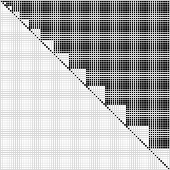
Figure 2: Display of the $\zeta$ = $90\times 90)$. The subposet $P_{t}$ of the $N$ i.e. integers sequence $N$-cobweb poset. $t=?$

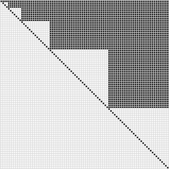
Figure 3: Display of the $\zeta$ = $90\times 90)$. The subposet $P_{t}$ of the $F$ = Gaussian integers sequence $(q=2)$. $F$-cobweb poset.$t=?$

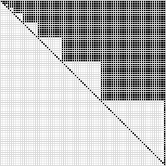
Figure 4: Display of the $\zeta$ = $90\times 90)$. The subposet $P_{t}$ of the $F$ = Fibonacci-cobweb poset.$t=?$

Remark 2. Krot Choice. While the above is established it is a matter of simple observation by inspection to find out how does the the Möbius matrix $\mu=\zeta^{-1}$ looks like. Using in [25,26] this author example and expression for $\zeta$ matrix this has been accomplished first (see also [26]) for Fibonacci sequence and then - via automatic extension - the same formula was given for $F$ sequences as above by my former student in her recent articles [27,28]. Here is her formula for the cobweb posets’ Möbius function (see: (6) in [28]).

$$\mu(x,y)=\mu(\left\langle s,t\right\rangle,\left\langle u,v\right\rangle)=\delta(s,u)\delta(t,v)-\delta(t+1,v)+\sum_{k=2}^{\infty}\delta(t+k,v)(-1)^{k}\prod_{i=t+1}^{v-1}F_{i}-1$$

Now bearing in mind the Upside Down Notation Principle for all $F$-cobweb posets with $F_{0}>0$ (as it should be for natural numbers valued sequences) we may now rewrite the above in coordinate grid $Z\times Z$ as below.

Let $x=\left\langle s,t\right\rangle$ and $y=\left\langle u,v\right\rangle$ where $1\leq s\leq F_{t}$, $1\leq u\leq F_{v}$ while $t,v\in N$. Then

$$\mu(x,y)=\mu(\left\langle s,t\right\rangle,\left\langle u,v\right\rangle)=\delta(s,u)\delta(t,v)+\sum_{k=1}^{\infty}\delta(t+k,v)(-1)^{k}\prod_{i=t+1}^{v-1}(i-1)_{F}$$

The further relevant references of the same author see [27-29]. The above rewritten Möbius function formula is of course literally valid for all natural numbers valued sequences $F$. Consult: the recent note ”‘On Characteristic Polynomials of the Family of Cobweb Posets”’ [29].

The author of [25] introduces parallely also another form of $\zeta$ function formula and since now on -except for [27]- in subsequent papers [26,28,29] their author uses the formula for $\zeta$ function in this another form. Namely - this other form formula for $\zeta$ function in the present authors’ grid coordinate system description of the cobweb posets was given by Krot in her note on Möbius function and Möbius inversion formula for Fibonacci cobweb poset [23] with $F$ designating the Fibonacci cobweb posets. In [24] the formula for the Möbius function for Fibonacci sequence $F$ was rightly treated as literally valid for all natural numbers valued sequences $F$ and the alternative. Of course the same concerns the $\zeta$ function formulas - the former and the latter. Here is this other latter form formula for $\zeta$ function (see: (7) in [25] or (1) in [27]).

Let $x=\left\langle s,t\right\rangle$ and $y=\left\langle u,v\right\rangle$ where $1\leq s\leq F_{t}$, $1\leq u\leq F_{v}$ while $t,v\in N$. Then

$$\zeta(x,y)=\zeta(\left\langle s,t\right\rangle,\left\langle u,v\right\rangle)=\delta(s,u)\delta(t,v)+\sum_{k=1}^{\infty}\delta(t+k,v)$$

where here - recall ($a,b\in Z$):

$$\delta(a,b)=\left\{\begin{array}[]{cl}1&for\ a=b,\\ 0&otherwise.\par\end{array}\right.$$

Farewell interactive question. Are then all the presented $\zeta$ incidence function matrix of $F$- denominated cobweb posets equivalent?

6 Appendix [42]

Cobweb posets and KoDAGs’ ponderables of the authors relevant productions.

Definition 6.1.

Let $n\in N\cup\left\{0\right\}\cup\left\{\infty\right\}$. Let $r,s\in N\cup\left\{0\right\}$. Let $\Pi_{n}$ be the graded partial ordered set (poset) i.e. $\Pi_{n}=(\Phi_{n},\leq)=(\bigcup_{k=0}^{n}\Phi_{k},\leq)$ and $\left\langle\Phi_{k}\right\rangle_{k=0}^{n}$ constitutes ordered partition of $\Pi_{n}$. A graded poset $\Pi_{n}$ with finite set of minimal elements is called cobweb poset iff

$$\forall x,y\in\Phi\ i.e.\ x\in\Phi_{r}\ and\ y\in\Phi_{s}\ r\neq s\ \Rightarrow\ x\leq y\ or\ y\leq x,$$

$\Pi_{\infty}\equiv\Pi.$

Note. By definition of $\Pi$ being graded its levels $\Phi_{r}\in\left\{\Phi_{k}\right\}_{k}^{\infty}$ are independence sets and of course partial order $\leq$ up there in Definition 6.1. might be replaced by $<$.

The Definition 6.1. is the reason for calling Hasse digraph $D=\left\langle\Phi,\leq\cdot\right\rangle$ of the poset $(\Phi,\leq))$ a KoDAG as in Professor Kazimierz Kuratowski native language one word Komplet means complete ensemble - see more in [23] and for the history of this name see: The Internet Gian-Carlo Polish Seminar Subject 1. oDAGs and KoDAGs in Company (Dec. 2008).

Definition 6.2.

Let $F=\left\langle k_{F}\right\rangle_{k=0}^{n}$ be an arbitrary natural numbers valued sequence, where $n\in N\cup\left\{0\right\}\cup\left\{\infty\right\}$. We say that the cobweb poset $\Pi=(\Phi,\leq)$ is denominated (encoded=labelled) by $F$ iff $\left|\Phi_{k}\right|=k_{F}$ for $k=0,1,...,n.$

Acknowledgments Thanks are expressed here to the now Student of Gdańsk University Maciej Dziemiańczuk for applying his skillful TeX-nology with respect to most of my articles since three years as well as for his general assistance and cooperation on KoDAGs investigation. Maciej Dziemiańczuk was not allowed to write his diploma with me being supervisor - while Maciej studied in the local Bialystok University where my professorship till 2009-09-30 comes from.

References

- [1] L. Colucci, O.M. D’Antona, C. Mereghetti: Fibonacci and Lucas Numbers as Cumulative Connection Constants”, The Fibonacci Quaterly 38.2 (2000), pp.157-164
- [2] E.Damiani,O.M. D’Antona, G. Naldi On the Connection Constants,Studies in Appl. Math. 85(4)(1991), pp. 289-302
- [3] A. Di Bucchianico ,D. Loeb: Sequences of Binomial type with Persistent Roots, J. Math. Anal. Appl. 199(1996),pp. 39-58
- [4] Goldman J. Rota G-C.: On the Foundations of Combinatorial Theory IV; Finite-vector spaces and Eulerian generating functions Studies in Appl. Math. vol. 49 1970, pp. 239-258
- [5] J.Konvalina: Generalized binomial coefficients and the subset-subspace problem, Adv. in Appl. Math. Vol. 21 (1998), pp. 228-240
- [6] J. Konvalina: A Unified Interpretation of the Binomial Coefficients, the Stirling Numbers and the Gaussian Coefficients, The American Mathematical Monthly vol. 107, No 10 , (2000), pp.901-910
- [7] Ward M.: A calculus of sequences, Amer.J. Math. 58 (1936) pp. 255-266
- [8] A. K. Kwaśniewski: Main theorems of extended finite operator calculus, Integral Transforms and Special Functions Vol 14 , No 6, (2003),pp. 499-516
- [9] A.K.Kwaśniewski: Towards -extension of Finite Operator Calculus of Rota, Rep. Math. Phys.48 No 3 (2001)pp. 305-342
- [10] A.K.Kwaśniewski: On Simple Characterisations of Sheffer -polynomials and Related Propositions of the Calculus of Sequences, Bulletin de la Soc. des Sciences et de Lettres de Lodz ; 52, Ser. Rech. Deform. 36 (2002) 45-65. ArXiv:math.CO/0312397
- [11] S.R.Roman: More on the umbral calculus with emphasis on the q-umbral calculus, J. Math. Anal. Appl. 107(1985), pp. 222-254
- [12] A.K.Kwaśniewski: Information on combinatorial interpretation of Fibonomial coefficients,Inst. Comp. Sci. UwB/PreprintNo52/November/2003, , Bull. Soc. Sci. Lett. Lodz Ser. Rech. Deform. 53, Ser. Rech.Deform. 42 (2003) pp. 39-41 ArXiv: math.CO/0402291 v 1 22 Feb 2004
- [13] A.K.Kwaśniewski: On extended finite operator calculus of Rota and quantum groups, Integral Transforms and Special Functions, Vol. 2, No.4(2001) pp. 333-340.
- [14] O.V. Viskov: Operator characterization of generalized Appel polynomials, Soviet Math. Dokl. 16 (1975),pp. 1521-1524
- [15] A. K. Kwaśniewski: On duality triads, Bull. Soc. Sci.Lett. Lodz Ser. Rech. Deform. 53, Ser. Rech.Deform. 42 (2003) pp.11-25 ArXiv: math.GM/0402260 v 1 Feb. 2004 ; A. K. Kwaśniewski: The second part of on duality triads‘ paper Bull. Soc. Sci. Lett. Lodz Ser. Rech. Deform. 53, Ser. Rech.Deform. 42 (2003) pp.27 -37 ArXiv: math.GM/0402288 v 1 Feb. 2004
- [16] A.K.Kwaśniewski: Combinatorial interpretation of the recurrence relation for fibonomial coefficients, Bulletin de la Societe des Sciences et des Lettres de Lodz (54) Serie: Recherches sur les Deformations Vol. 44 (2004) pp. 23-38, arXiv:math/0403017v2 [v1] Mon, 1 Mar 2004 02:36:51 GMT
- [17] A. Krzysztof Kwaśniewski, On cobweb posets and their combinatorially admissible sequences, Adv. Studies Contemp. Math. Vol. 18 (1), 2009 Vol. 18 No 1, 2009 17-32. arXiv:math/0512578v4 [v1] Mon, 26 Dec 2005 20:12:57 GMT
- [18] A. Krzysztof Kwaśniewski, More on combinatorial interpretation of fibonomial coefficients, Inst. Comp. Sci.UwB/PreprintNo56/November/2003, Bulletin de la Societe des Sciences et des Lettres de Lodz (54) Serie: Recherches sur les Deformations Vol. 44 (2004) pp. 23-38, arXiv:math/0402344v2 [v1] 23 Feb 2004 Mon, 20:27:13 GMT
- [19] A. Krzysztof Kwaśniewski, Cobweb posets as noncommutative prefabs, Adv. Stud. Contemp. Math. vol. 14 (1) (2007) 37-47. arXiv:math/0503286v4 ,[v1] Tue, 15 Mar 2005 04:26:45 GMT
- [20] A. Krzysztof Kwaśniewski, How the work of Gian Carlo Rota had influenced my group research and life, arXiv:0901.2571v1 [v4] Tue, 10 Feb 2009 03:42:43 GMT
- [21] A. Krzysztof Kwaśniewski Graded posets zeta matrix formula arXiv:0901.0155v1 [v1] Thu, 1 Jan 2009 01:43:35 GMT the 15 pages Sylvester Night paper
- [22] A. Krzysztof Kwaśniewski On cobweb posets and their combinatorially admissible sequences Adv. Studies Contemp. Math. Vol. 18 No 1, 2009 17-32. arXiv:math/0512578v4 [v1] Mon, 26 Dec 2005 20:12:57 GMT
- [23] A. Krzysztof Kwaśniewski, Cobweb Posets and KoDAG Digraphs are Representing Natural Join of Relations, their diBigraphs and the Corresponding Adjacency Matrices, arXiv:0812.4066v1 [v1] Sun, 21 Dec 2008 the 19 pages Chistmas Eve article
- [24] A. Krzysztof Kwaśniewski, Some Cobweb Posets Digraphs’ Elementary Properties and Questions, arXiv:0812.4319v1 [v1] Tue 23 Dec 2008 the 6 pages Christmas Eve letter
- [25] Ewa Krot A note on Möbius function and Möbius inversion formula of fibonacci cobweb poset, Bulletin de la Societe des Sciences et des Lettres de Lodz (54), Serie: Recherches sur les Deformations Vol. 44 (2004), 39-44 arXiv:math/0404158v2, [v1] Wed, 7 Apr 2004 10:23:38 GMT [v2] Wed, 28 Apr 2004 07:37:14 GMT
- [26] Ewa Krot The First Ascent into the Incidence Algebra of the Fibonacci Cobweb Poset, Advanced Studies in Contemporary Mathematics 11 (2005), No. 2, 179-184, arXiv:math/0411007v1 [v1] Sun, 31 Oct 2004 12:46:51 GMT
- [27] Ewa Krot-Sieniawska, On incidence algebras description of cobweb posets, arXiv:0802.3703v1 [v1] Tue, 26 Feb 2008 13:12:43 GMT
- [28] Ewa Krot-Sieniawska, Reduced Incidence algebras description of cobweb posets and KoDAGs, arXiv:0802.4293v1, [v1] Fri, 29 Feb 2008 05:43:27 GMT
- [29] Ewa Krot-Sieniawska, On Characteristic Polynomials of the Family of Cobweb Posets,Proc. Jangjeon Math. Soc. Vol11 (2008) no. 2. pp.105-111 arXiv:0802.2696v1 [v1] Tue, 19 Feb 2008 18:53:38 GMT
- [30] Donald E. Knuth Two Notes on Notation, Amer. Math. Monthly 99 (1992), no. 5, 403-422 , arXiv:math/9205211v1, [v1] Fri, 1 May 1992 00:00:00 GMT
- [31] A. Krzysztof Kwaśniewski, M. Dziemiańczuk, Cobweb posets - Recent Results, Adv. Stud. Contemp. Math. vol. 16 (2) April 2008 . pp. 197-218; arXiv:math/0801.3985, 25 Jan 2008
- [32] A. Krzysztof Kwaśniewski, Ewa Krot-Sieniawska, On inversion formulas and Fibonomial coefficients, Proc. Jangjeon Math. Soc, 11 (1), 2008 (June), ArXiv:0803.1393 10 Mar 2008
- [33] A. K. Kwaśniewski, M. Dziemiańczuk, On cobweb posets’ most relevant codings, ArXiv:0804.1728v1 10 Apr 2008
- [34] M. Dziemiańczuk, On Cobweb posets tiling problem, Adv. Stud. Contemp. Math. volume 16 (2), 2008 (April) pp. 219-233, ArXiv:0709.4263 4 Oct 2007
- [35] M. Dziemiańczuk, On Cobweb Admissible Sequences - The Production Theorem, The 2008 International Conference on Foundations of Computer Science (FCS’08: WORLDCOMP’08, USA, Las Vegas)
- [36] M. Dziemiańczuk, Report On Cobweb Posets’ Tiling Problem,t ArXiv:0802.3473v1 27 Feb 2008
- [37] M. Dziemiańczuk, Report On Cobweb Posets’ Tiling Problem, Preprint: arXiv:0802.3473v1, 27 Feb 2008
- [38] M. Dziemianczuk, On multi F-nomial coefficients and Inversion formula for F-nomial coefficients, Preprint: arXiv:0806.3626, 23 Jun 2008
- [39] M. Dziemiańczuk, W.Bajguz, On GCD-morphic sequences, Preprint arXiv:0802.1303v1, 10 Feb 2008
-
[40]
M.Dziemiańczuk, Cobweb Posets Website,
http://www.faces-of-nature.art.pl/cobwebposets.html - [41] A. Krzysztof Kwaśniewski Fibonomial cumulative connection constants Inst. Comp. Sci. UwB/PreprintNo58/December/2003, ,Bulletin of the ICA vol. 44 (2005), 81-92
- [42] A. Krzysztof Kwaśniewski Graded posets inverse zeta matrix formula to appear