A numerical method for constructing the hyperbolic structure of complex Hénon mappings

Abstract.

For complex parameters $a,c$, we consider the Hénon mapping $H_{a,c}:\mathbb{C}^{2}\rightarrow\mathbb{C}^{2}$, given by $(x,y)\mapsto(x^{2}+c-ay,x)$, and its Julia set, $J$. In this paper, we describe a rigorous computer program for attempting to construct a cone field in the tangent bundle over $J$, which is preserved by $DH$, and a continuous norm in which $DH\ (\text{and }DH^{-1})$ uniformly expands the cones (and their complements). We show a consequence of a successful construction is a proof that $H$ is hyperbolic on $J$. We give several new examples of hyperbolic maps, produced with our computer program, Hypatia, which implements our methods.

1. Introduction

The Hénon family, $H_{a,c}(x,y)=(x^{2}+c-ay,x)$, has been extensively studied as a diffeomorphism of $\mathbb{R}^{2}$, with $a,c$ real parameters. For example, Benedicks and Carleson show the existence of chaotic behavior in the form of a strange attractor for some real Hénon maps in [8]. Here we consider $H_{a,c}$ as a diffeomorphism of $\mathbb{C}^{2}$, and allow $a,c$ to be complex. Foundational work on the dynamics of the complex Hénon family has been done by Bedford and Smillie ([2, 3, 7, 4]), Hubbard ([22, 23, 21]), and Fornaess and Sibony ([14]). However, basic questions remain unanswered.

A natural class of maps to study are the hyperbolic maps, since hyperbolic maps generally have nontrivial (chaotic) dynamics, but are amenable to analysis. A Hénon mapping $H_{a,c}$ is hyperbolic if its Julia set, $J_{a,c}$, is a hyperbolic set for $H_{a,c}$. (Hyperbolicity and Julia set are defined in Section 2.) For Hénon mappings, hyperbolicity implies Axiom A, which implies shadowing on $J$, i.e., $\epsilon$-pseudo orbits are $\delta$-close to true orbits, and structural stablity on $J$, i.e., in a neighborhood in parameter space the dynamical behavior is of constant topological conjugacy type. Thus for a hyperbolic mapping, the dynamics on $J$ should be able to be understood using combinatorial models. These properties make hyperbolic diffeomorphisms amenable to exploration via computers.

Motivated by careful computer investigations, Oliva ([32]) provides a combinatorial model of the dynamics of some Hénon mappings, including for example, the mapping of Figure 1. The proposed model presupposes that the mapping is hyperbolic.

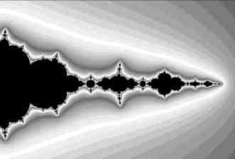
Figure 1. The filled Julia set for a Hénon mapping $H_{a,c}(x,y)$ $=$ $(x^{2}+c-ay,x)$, restricted to the unstable manifold of a saddle fixed point, with its natural parameterization. Here $a=.3,c=-1.17$, and the map has attracting cycles of periods one and three, which is impossible for quadratic polynomial maps of $\mathbb{C}$.

Hubbard and Papadantonakis ([1, 20]) have more recently generated pictures of slices of the Hénon parameter space, which attempt to sketch either the locus of maps with $J$ connected, or the locus of maps with $J$ having no interior (see Figure 2).

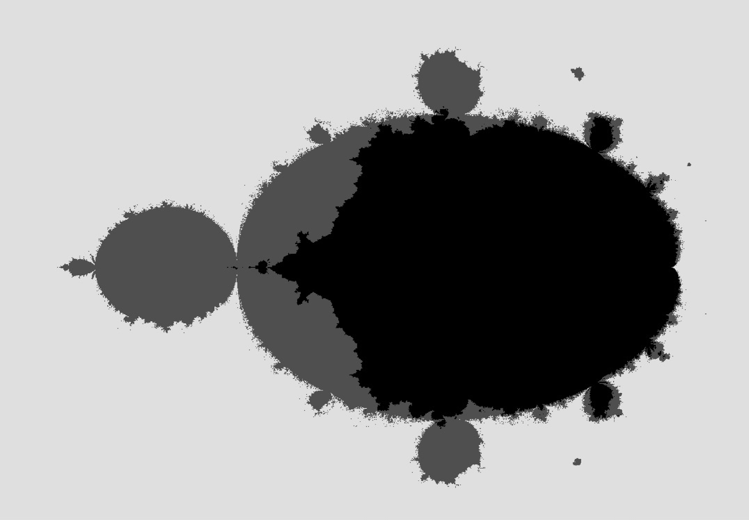
Figure 2. A slice of Hénon parameter space, the $c$-plane, with $a=.3$. The innermost dark set is an attempt to sketch the set of maps with connected Julia sets, while the exterior is an attempt to sketch the maps with filled Julia set having empty interior (including complex horseshoes). These regions have features reminiscent of the parameter regions of one-dimensional polynomial maps. This is an intriguing parallel, suggesting that the Hénon parameter space may be an equally rich arena of study.

These and other computer investigations suggest that the dynamical behavior of the complex Hénon family is rich and subtle. If certain of these mappings could be shown to be hyperbolic, then this would serve as a first step toward showing mathematically that these apparent phenomena actually occur.

However, there are very few complex Hénon mappings known to be hyperbolic. Let us summarize what is known. First, if

(1) $$\left\lvert c\right\rvert>2(1+\left\lvert a\right\rvert)^{2},$$

then $H_{a,c}|_{J}$ is conjugate to the full 2-shift (so $J_{a,c}$ is a Cantor set), and the map is hyperbolic (compare Devaney and Nitecki [12], Oberste-Vorth [31], Morosawa, et al. [28]). In this case the mapping is called a (complex) horseshoe. The exterior in Figure 2 contains the set of horseshoes (among other types of maps). Second, Hubbard and Oberste-Vorth ([23]) show that if $P_{c}(x)=x^{2}+c$ is a hyperbolic polynomial, then there exists an $A(c)$ such that if

(2) $$0<~{}\left\lvert a\right\rvert~{}<A(c),$$

then $H_{a,c}|_{J}$ is topologically conjugate to the function induced by $P_{c}$ on the inverse limit ${\lim_{\leftarrow}(J,P_{c})}$, hence $H_{a,c}$ is hyperbolic. Ishii and Smillie ([24]) have worked to obtain explicit estimates for the constant $A(c)$ in (2), but these estimates are relatively small.

Our broad goal is to develop computer algorithms with which we can rigorously describe the dynamics of any hyperbolic complex Hénon mapping. In this paper we make a key step in that process, by developing a computer program which can establish if a complex Hénon mapping is hyperbolic, and if so, the program produces explicit information about how the map is hyperbolic; in particular, it builds two complementary cone fields in the tangent bundle over $J$ (the unstable and stable cones), and constructs a norm in which $DH\ (DH^{-1})$ preserves and unifomly expands the unstable (stable) cones.

Since hyperbolicity is structurally stable, a computer program with infinite resources should be able to prove hyperbolicity for any hyperbolic map. However, non-hyperbolicity is an unstable condition, thus a computer program cannot be expected to recognize when a map is not hyperbolic. (For example, $P(z)=z^{2}-1.5$ is presumably, but not provably, non-hyperbolic.)

This paper builds on the results of [18] (cf [25, 11, 33, 34, 13]). There we describe an algorithm, called the box chain construction, which given $\epsilon>0$ finds a compact neighborhood, $\mathcal{B}$, containing a $\delta=\delta(\epsilon)$-neighborhood of $J$, and creates a finite graph, $\Gamma$, which models the $\epsilon$-dynamics of $H$ on $\mathcal{B}$. In this paper, we need only know the following about $\Gamma$.

Definition 1.1.

Let $\Gamma=\Gamma(\mathcal{V},\mathcal{E})$ be a directed graph, with vertex set $\mathcal{V}=\{B_{k}\}_{k=1}^{N}$ a finite collection of closed boxes in $\mathbb{C}^{2}$, having disjoint interiors, and such that the union of the boxes $\mathcal{B}=\cup_{k=1}^{N}B_{k}$ contains $J$. Suppose there is a $\delta>0$ such that $\Gamma$ contains an edge from $B_{k}$ to $B_{j}$ if the image $H(B_{k})$ intersects a $\delta$-neighborhood of $B_{j}$, i.e.,

$$\mathcal{E}\supset\{(k,j)\colon H(B_{k})\cap\mathcal{N}(B_{j},{\delta})\neq\emptyset\}.$$

Further, assume $\Gamma$ is strongly connected, i.e., for each pair of vertices $B_{k},B_{j}$, there is a path in $\Gamma$ from $B_{k}$ to $B_{j}$, and vice-versa. Then we call $\Gamma$ a box chain model of $H$ on $J$.

In [18], we describe how the box chain construction builds strongly connected graphs modeling every basic set of $H$, for example, $J$ and any attracting periodic orbits. In this paper, we let $\Gamma$ be the strongly connected graph component containing $J$, and we mostly ignore the others.

Our first task in this paper is to develop a discrete condition on $\Gamma$ we call box hyperbolicity, and show this condition implies hyperbolicity of $H$:

Theorem 1.2.

Let $\Gamma$ be a box chain model of $H$ on $J$. If $\Gamma$ is box hyperbolic, then $H$ is hyperbolic on $J$.

Our definition of box hyperbolicity is inspired by our work in numerically establishing hyperbolicity in one complex dimension (see [19]). The difference is that in one dimension, hyperbolicity simply means expansion on $J$, whereas for Hénon mappings, hyperbolicity means a saddle property, i.e., expansion, contraction, and transversality. The notion of box hyperbolicity is made precise in Section 4. Let us briefly describe this property here. We begin with the cone field criterion for hyperbolicity. In a more general setting, Newhouse and Palis ([29, 30]) show that an $f$-invariant set $\Lambda$ is hyperbolic for $f$ iff there is a field of cones in the tangent bundle over $\Lambda$ such that $Df$ maps the cone field inside itself, and such that in some norm, $Df$ uniformly expands the cones, and $Df^{-1}$ uniformly expands the complements of the cones. Moreover, the field of cones need not be continuous in $x\in\Lambda$; hence the cone field criterion for hyperbolicity yields a natural way to study the hyperbolic structure of a diffeomorphism using a computer (i.e., discretely). Here, we build cones which are constant on each box vertex of $\Gamma$.

To use the cone field criterion, we must find both a field of cones preserved by $DH$ and a norm in which $DH$ expands the cones. We cannot expect that $DH$ expands vectors in each cone with respect to the euclidean norm. For example, in the euclidean norm, $DH$ may be small for some cones over a pseudo-cycle, but larger in others, so that only the total cycle multiplier is larger than one. Thus given a model $\Gamma$ of a map $H$, we attempt to build a discretized norm on the tangent bundle over $\Gamma$, which is designed to factor out the differences in $DH$ along cycles, so that in this new norm, $DH$ is expanding on every cone. Then we show that hyperbolicity in the discrete norm implies hyperbolicity for some continuous norm.

In order to test for box hyperbolicity on a given $\Gamma$, we have developed a computer algorithm we call the Axis Metric Algorithm, designed to either prove that a given $\Gamma$ is box hyperbolic, or describe which parts of $\Gamma$ are obstructions to proving box hyperbolicity. If a $\Gamma$ fails to be box hyperbolic, then either the map is not hyperbolic, or the boxes of $\Gamma$ are too large. Thus our approach is to attempt to prove box hyperbolicity on a sequence of models $\Gamma(n)$ with decreasing box size. If $\Gamma(n-1)$ fails to be box hyperbolic, then to create $\Gamma(n)$ we could decrease the size of all the boxes, or use output of the Axis Metric Algorithm on $\Gamma(n-1)$ in choosing which boxes need to be decreased in order to create a $\Gamma(n)$ more likely to be box hyperbolic. If some $\Gamma(n)$ is found to be box hyperbolic, then $f$ is hyperbolic, and the program terminates. Thus a “successful” run of an implementation of our procedure gives a mathematical proof of hyperbolicity: if we can construct a $\Gamma$ which the Axis Metric Algorithm shows to be box hyperbolic, then that mapping is mathematically proven to be hyperbolic, by Theorem 1.2.

In designing the Axis Metric Algorithm for verifying box hyperbolicity of some $\Gamma$, we build on the one-dimensional procedure described in [19]. There we prove hyperbolicity of polynomial maps of $\mathbb{C}$ by creating a piecewise continuous (box constant) metric, under which the map is expanding on a neighborhood of $J$. To move up to two dimensions, and saddle-type hyperbolicity, we break down the problem into one dimensional pieces, then reassemble. In particular, we build approximately invariant, box constant unstable and stable line fields, which will serve as axes for our cones. Then we use the one dimensional algorithm twice, to attempt to build a metric which is contracted on the stable directions, and another metric which is expanded on the unstable directions. These metrics and line fields then determine a cone field with an induced metric, which we use to test for box hyperbolicity. The Axis Metric Algorithm is described in detail in Section 5.

Finally, we have implemented our methods into a computer program called Hypatia, and used the program to prove hyperbolicity of several Hénon mappings which were not previously known to be hyperbolic:

Theorem 1.3.

The complex Hénon mappings, $H_{a,c}(x,y)=$ $(x^{2}+c-ay,x)$, with:

$$(c,a)=(-0.3,0.1),(0,-0.22),(-3,-0.25),\text{ and }(1.5,0.5),$$

are hyperbolic.

Computer pictures suggest that the first two mappings of Theorem 1.3, $H_{a,c}$ with $(c,a)=(-.3,.1)$ and $(c,a)=(0,-.22)$, are in the main cardioid, with the only recurrent dynamics consist of a connected $J$ and one attracting fixed point, and that the latter two mappings are horseshoes, with $J_{a,c}$ with $c=-3,a=-.25$ appearing to lie in $\mathbb{R}^{2}$, and $J_{a,c}$, with $c=1.5,a=.5$ appearing not to be contained in $\mathbb{R}^{2}$. Whether or not that is the case, each of the maps of Theorem 1.3 lies outside of the known regions defined by (1) and (2) with the Ishii-Smillie estimates.

All of the computations involved in proving Theorem 1.3 were run on a Sun Enterprise E3500 server with 4 processors, each $400$MHz UltraSPARC (though the multiprocessor was not used) and $4$ GB of RAM. When computations became overwhelming, memory usage was the limiting factor. The C++, unix program, Hypatia, may be obtained from the author.

To conclude the introduction, we sketch the organization of the paper. We give background on the dynamics of the Hénon family in Section 2. In Section 3, we briefly discuss interval arithmetic with directed rounding, the method used to maintain rigor in our computer computations. In Section 4, we define box hyperbolicity, and we prove Theorem 1.2, establishing that box hyperbolicity implies hyperbolicity. In Section 5, we describe our computer procedure for verifying box hyperbolicity, including the Axis Metric Algorithm. Finally, in Section 6 we provide some data on how we used Hypatia to prove hyperbolicity of each of the maps of Theorem 1.3.

Acknowledgements. These results were primarily accomplished as my PhD thesis at Cornell University ([17]). I am grateful to John Smillie for providing guidance on the project, John Hubbard for inspiration, Greg Buzzard, and Warwick Tucker for many helpful conversations, Eric Bedford, James Yorke, and John Milnor for advice on the preparation of this paper, and Robert Terrell for technical support. I would also like to thank the referees and editors for providing comments which I helped me to significantly increase the clarity of the presentation.

2. Background

2.1. The Hénon Family

Polynomial diffeomorphisms of $\mathbb{C}^{2}$ necessarily have polynomial inverses, thus are often called polynomial automorphisms. Friedland and Milnor ([15]) showed that polynomial automorphisms of $\mathbb{C}^{2}$ break down into two categories. Elementary automorphisms have simple dynamics, and are polynomially conjugate to a diffeomorphism of the form $(x,y)\mapsto(ax+b,cy+p(x))$ ($p$ polynomial, $a,c\neq 0$). Nonelementary automorphisms are all conjugate to finite compositions of generalized Hénon mappings, which are of the form $f(x,y)=(p(x)-ay,x)$, where $p(x)$ is a monic polynomial of degree $d>1$ and $a\neq 0$.

To clarify the situation, one can define a dynamical degree of a polynomial automorphism of $\mathbb{C}^{2}$. If deg$(f)$ is the maximum of the degrees of the coordinate functions, the dynamical degree is

$$d=d(f)=\lim_{n\to\infty}(\textit{deg}(f^{n}))^{1/n}.$$

This degree is a conjugacy invariant. Elementary automorphisms have dynamical degree $d=1$. A nonelementary automorphism is conjugate to some automorphism whose polynomial degree is equal to its dynamical degree. Without loss of generality, we assume such $f$ are finite compositions of generalized Hénon mappings, rather than merely conjugate to mappings of this form.

Thus, the quadratic, complex Hénon family $H_{a,c}(x,y)=(x^{2}+c-ay,x)$ represents the dynamical behavior of the simplest class of nonelementary polynomial automorphisms; those of dynamical degree two. In this paper, we usually use the letter $f$ for a polynomial diffeomorphism of $\mathbb{C}^{2}$ with $d(f)>1$, and $H$ for a (degree two) Hénon mapping. We state results in Section 4 for the more general $f$, but in explaining the procedure for verifying hyperbolicity in Section 5, we concentrate on the case of $H_{a,c}$.

2.2. Drawing Meaningful Pictures

For a polynomial map $P$ of $\mathbb{C}$, the filled Julia set, $K$, is the set of points whose orbits are bounded under $P$; the Julia set, $J$, is the topological boundary of $K$. For a polynomial diffeomorphism $f$, like $H_{a,c}$, there are corresponding Julia sets:

• $K^{+}(K^{-})$ is the set of points whose orbits are bounded under $f(f^{-1})$
  and $K=K^{+}\cap K^{-}$ is called the filled Julia set;

• $J^{\pm}=\partial K^{\pm}$ (topological boundary)
  and $J=J^{+}\cap J^{-}$ is called the Julia set.

Filled Julia sets are the (chaotic) invariant sets which can be easily sketched by computer, on any two-dimensional slice. Hubbard has suggested the following method for drawing a dynamically significant slice of the Julia set, by parameterizing an unstable manifold. This method has been implemented by Karl Papadantonakis in FractalAsm ([20, 1]). Figures 1, 4, and 5 were generated using FracalAsm.

Let $f$ be a diffeomorphism of $\mathbb{C}^{2}$. If $p$ is a periodic point of period $m$, and the eigenvalues $\lambda,\mu$ of $D_{p}f^{m}$ satisfy $\left\lvert\lambda\right\rvert>1>\left\lvert\mu\right\rvert$ (or vice-versa), then $p$ is a saddle periodic point. The large (small) eigenvalue is called the unstable (stable) eigenvalue. If $p$ is a saddle periodic point, then the stable manifold of $p$ is $W^{s}(p)=\{q\colon d(f^{n}(q),f^{n}(p))\rightarrow 0\text{ as }n\rightarrow\infty\},$ and the unstable manifold of $p$ is $W^{u}(p)=\{q\colon d(f^{-n}(q),f^{-n}(p))\rightarrow 0\text{ as }n\rightarrow\infty\}.$ If $p$ a saddle periodic point of $f$, then $W^{u}(p)\ (W^{s}(p))$ is biholomorphically equivalent to $\mathbb{C}$, and on $W^{u}(p)\ (W^{s}(p))$, $f$ is conjugate to multiplication by the unstable (stable) eigenvalue of $D_{p}f$.

When $\left\lvert a\right\rvert\neq 1$, except on the curve of equation $4c=(1+a)^{2}$, the map $H_{a,c}$ has at least one saddle fixed point, $p$, ([20]). The unstable manifold $W^{u}(p)$ has a natural parametrization $\gamma\colon\mathbb{C}\to W^{u}(p)$ given by

$$\gamma(z)=\lim_{m\to\infty}\gamma_{m}(z)=\lim_{m\to\infty}H^{m}\left(p+\frac{z}{\lambda_{1}^{m}}\mathbf{v_{1}}\right),$$

where $\lambda_{1}$ is the unstable eigenvalue of $D_{p}H$ and $\mathbf{v_{1}}$ is the associated eigenvector. This parametrization has the property that $H(\gamma(z))=\gamma(\lambda z),$ and any two parametrizations with this property differ by scaling the argument.

Observe that since $W^{u}(p)\subset K^{-}$, to get a picture of $K$ in $W^{u}(p)$ we need only color pixels black which are guessed to be in $K^{+}$. To sketch the picture, we approximate $\gamma$ by say $g=\gamma_{100}$ in a region in the plane, $B=\{z=x+iy\colon a\leq x\leq b,c\leq y\leq d\}$. Then an escape threshold is chosen, like $10$, and then for each $z\in B$, if $\left\|H^{n}(g(z))\right\|<10$ for all $n<100$, we say $g(z)\in K^{+}$ and color it black. Otherwise, color according to which iterate $\left\|H^{n}(g(z))\right\|$ first surpassed $10$.

2.3. Hyperbolicity

In this subsection, let $f$ be a diffeomorphism of a manifold $M$, and let $\Lambda$ be a compact, $f$-invariant set. First we recall the standard definition of hyperbolicity (see [36]).

Definition 2.1.

$\Lambda$ is hyperbolic for $f$ if at each $x$ in $\Lambda$, there is a splitting of the tangent bundle $T_{x}M=E^{s}_{x}\oplus E^{u}_{x}$, which varies continuously with $x\in\Lambda$, such that:

1. $f$ preserves the splitting, i.e., $D_{x}f(E^{s}_{x})=E^{s}_{fx}$, and $D_{x}f(E^{u}_{x})=E^{u}_{fx}$, and

2. $Df\ (Df^{-1})$ expands on $E^{u}\ (E^{s})$ uniformly, i.e., there exists a constant $\lambda>1$ and a norm $\left\|\cdot\right\|_{x}$ on $T_{\Lambda}M$, continuous for $x\in\Lambda$, for which

   $$\left\|D_{x}f(\mathbf{w^{u}})\right\|_{f(x)} \geq \lambda\left\|\mathbf{w^{u}}\right\|_{x},\text{ for }\mathbf{w^{u}}\in E^{u}_{x},\text{ and }$$

   $$\left\|D_{x}f^{-1}(\mathbf{w^{s}})\right\|_{f^{-1}(x)} \geq \lambda\left\|\mathbf{w^{s}}\right\|_{x},\text{ for }\mathbf{w^{s}}\in E^{s}_{x}.$$

As noted in the Introduction, Newhouse and Palis ([29, 30]) show hyperbolicity can be described using a cone field. To define a cone $C_{x}$ for each point $x$ in $\Lambda$, we need a splitting $T_{x}M=E_{1x}\oplus E_{2x}$, and a positive real-valued function $\epsilon(x)$ on $M$. Then define the $\epsilon(x)$-sector $S_{\epsilon(x)}(E_{1x},E_{2x})$ by

$$S_{\epsilon(x)}(E_{1x},E_{2x})=\{(\mathbf{v}_{1},\mathbf{v}_{2})\in E_{1x}\oplus E_{2x}:\left\|\mathbf{v}_{2}\right\|\leq\epsilon(x)\left\|\mathbf{v}_{1}\right\|\}.$$

Then $C_{x}=S_{\epsilon(x)}$. Newhouse and Palis show that $\Lambda$ is hyperbolic for $f$ iff there is a field of cones $\{C_{x}\subset T_{x}M\colon x\in\Lambda\}$, a constant $\lambda>1$, and a continuous norm $\left\|\cdot\right\|$, such that $Df$ preserves the cone field, i.e., $D_{x}f(C_{x})\subset C_{fx}$, and such that in this norm, $D_{x}f\ (D_{x}f^{-1})$ uniformly expands vectors in $C_{x}\ (T_{x}M-C_{x})$; moreover, the field of cones $x\rightarrow C_{x}$ need not be continuous. Our computer algorithm for verifying hyperbolicity actually combines these two notions, as we will see in Section 4.

Bedford and Smillie ([6]) have shown that for $f$ a polynomial diffeomorphism of $\mathbb{C}^{2}$, with $d(f)>1$, $f$ is hyperbolic on its Julia set, $J$, iff $f$ is hyperbolic on its chain recurrent set, $\mathcal{R}$, iff $f$ is hyperbolic on its nonwandering set, $\Omega$. Thus we say $f$ is hyperbolic if any of these conditions holds. In fact, in [5] Bedford and Smillie show that if $f$ is hyperbolic, then $\mathcal{R}$ and $\Omega$ are both equal to $J$ union finitely many attracting periodic orbits. Thus for hyperbolic polynomial diffeomorphisms of $\mathbb{C}^{2}$, the basic sets are $J$ and the attracting periodic orbits.

3. Interval arithmetic

In order to genuinely prove dynamical properties, we use in Hypatia a method of controlling round-off error in the computations, called interval arithmetic with directed rounding (IA). This method was recommended by Warwick Tucker, who used it in his recent computer proof that the Lorenz differential equation has the conjectured geometry ([37]).

In fact we use IA not only to control error, but we take advantage of the structure of this method in our algorithms and implementation. We thus give a very brief description of IA below, and refer the interested reader to [26, 27, 9].

On a computer, we cannot work with real numbers, rather we work over the finite space $\mathbb{F}$ of numbers representable by binary floating point numbers no longer than a certain length. For example, since the number $0.1$ is not a dyadic rational, it has an infinite binary expansion. The computer cannot encode this number exactly. Instead, the basic objects of arithmetic are not real numbers, but closed intervals, $[a,b]$, with end points in some fixed field $\mathbb{K}$. Denote this space of intervals by $\mathbb{I}\mathbb{K}$. The operation of addition of two intervals $[a,b],$ $[c,d]\in\mathbb{I}\mathbb{K}$ is defined by: $[a,b]+[c,d]=\left[a+c,b+d\right].$ Hence if $x\in[a,b]$ and $y\in[c,d]$, then $x+y\in[a,b]+[c,d]$.

The other operations are defined analogously, for example:

$$[a,b]-[c,d] =\left[a-d,b-c\right],\text{ and }$$

$$[a,b]\times[c,d] =\left[\min(ac,ad,bc,bd),\max(ac,ad,bc,bd)\right]$$

However, an arithmetical operation on two numbers in $\mathbb{F}$ may not have a result in $\mathbb{F}$. Thus to implement rigorous IA we use the idea of directed rounding to round outward the result of any operation. For example,

$$[a,b]+[c,d]=\left[\left\downarrow a+c\right\downarrow,\left\uparrow b+d\right\uparrow\right],$$

where $\left\downarrow x\right\downarrow$ is the largest number in $\mathbb{F}$ strictly less than $x$ (i.e., $x$ rounded down), and $\left\uparrow x\right\uparrow$ is the smallest number in $\mathbb{F}$ strictly greater than $x$ (i.e., $x$ rounded up). For any $x\in\mathbb{R}$, let Hull$(x)$ be the smallest interval in $\mathbb{I}\mathbb{F}$ which contains $x$. Thus, if $x\in\mathbb{F}$, then Hull$(x)=[x,x]$. If $x\in\mathbb{R}\setminus\mathbb{F}$, then Hull$(x)=[\left\downarrow x\right\downarrow,\left\uparrow x\right\uparrow]$.

Thus, if the user is interested in a computation involving real numbers, then IA with directed rounding performs the computation using intervals in $\mathbb{I}\mathbb{F}$ which contain those real numbers, and gives the answer as an interval in $\mathbb{I}\mathbb{F}$ which contains the real answer. In higher dimensions, IA operations can be carried out component-wise, on interval vectors.

One must think carefully about how to use IA in each arithmetical calculation. For example, it can create problems by propagating increasingly large error bounds. Iterating a polynomial diffeomorphism like $H_{a,c}$ on an interval vector which is not very close to an attracting period cycle will give a tremendously large interval vector after only a few iterates. That is, suppose $B=[a,b]\times[c,d]$ is an interval vector in $\mathbb{C}$, and one attempts to compute a box containing $P_{c}^{10}(B)$, for $P_{c}(z)=z^{2}+c$, by:

for $j$ from $1$ to $10$ do
	$B=P_{c}(B)$

then the box $B$ will likely grow so large that its defining bounds become machine $\infty$, i.e., the largest floating point in $\mathbb{F}$. Similarly, one would also never want to try to compute $D_{B_{n}}H\circ\cdots\circ D_{B_{1}}H\circ D_{B_{0}}H(\mathbf{u}),$ for a vector $\mathbf{u}\in\mathbb{C}^{2}$, since the entries would blow up (see Algorithm 5.1, Step 1).

Our construction involving boxes in $\mathbb{C}^{2}$ as the basic numerical objects is designed to be efficiently manipulated with IA. For all of our rigorous computations, we use IA routines provided by the PROFIL/BIAS package, available at [35].

4. Characterizing box hyperbolicity

In this section we define box hyperbolicity for a box chain model $\Gamma$, in Definition 4.1, and show that if $\Gamma$ is box hyperbolic, then $f$ satisfies the standard definition of hyperbolicity, proving Theorem 1.2. Further, we show in Proposition 4.11 that box hyperbolicity is equivalent to a simple condition in linear algebra. Throughout this section, assume $f$ is a polynomial diffeomorphism of $\mathbb{C}^{2}$, with $d(f)>1$, and let $\Gamma=(\mathcal{V},\mathcal{E})$ be a box chain model of $f$ on $J$.

Definition 4.1.

Suppose for each box $B_{k}$ in $\mathcal{V}$, we have some nondegenerate indefinite Hermitian form, $Q_{k}\colon\mathbb{C}^{2}\to\mathbb{R}$. Define ${C}^{u}_{k}:=\{\mathbf{w}\colon Q_{k}(\mathbf{w})\geq 0\}$, as the unstable cones, and define their complements as the stable cones: ${C}^{s}_{k}:=\mathbb{C}^{2}\setminus{C}^{u}_{k}=\{\mathbf{v}\colon Q_{k}(\mathbf{v})<0\}$.

We say that $\Gamma$ is box hyperbolic if $Df$ ($Df^{-1}$) preserves and expands the unstable (stable) cones, with respect to $\{Q_{k}\}$, i.e., for every edge $(k,j)\in\mathcal{E}(\Gamma)$, and every $z\in B_{k}$:

1. if $\mathbf{w}\in C^{u}_{k}$, then $D_{z}f(\mathbf{w})\in C^{u}_{j}$ and ${Q_{j}(D_{z}f(\mathbf{w}))}\ >\ {Q_{k}(\mathbf{w})};$

2. if $\mathbf{v}\in C^{s}_{j}$, then $\left[D_{z}f\right]^{-1}(\mathbf{v})\in C^{s}_{k}$ and $-{Q_{k}\left(\left[D_{z}f\right]^{-1}(\mathbf{v})\right)}\ >\ -{Q_{j}(\mathbf{v})}$.

In fact, a given cone $C^{u}_{k}$ determines an associated Hermitian form $Q_{k}$ up to scaling. Finding an appropriate choice of scaling for each $Q_{k}$ is how we determine a metric for which $H$ is hyperbolic. To prove Theorem 1.2, we first use a partition of unity argument to smooth out the forms $\{Q_{k}\}_{k=1}^{N}$ into a continuous field of forms $\{Q_{z}\}_{z\in J}$ (Definition 4.8), then define a riemannian metric induced by $\{Q_{z}\}_{z\in J}$ (Definition 4.10), and show that $H$ is hyperbolic on $J$ in this new riemannian metric.

4.1. Box hyperbolicity implies hyperbolicity

Here our goal is to prove Theorem 1.2, that if $\Gamma$ is box hyperbolic, then $f$ is hyperbolic on $J$, as in Definition 2.1. Part of the proof is very similar to the one dimensional analog, proved in [19], in that we use a partition of unity to smooth out a discrete norm. But before we deal with the norm, we verify that box hyperbolicity implies the existence of a continuous splitting preserved by the map.

Lemma 4.2.

If $\Gamma$ is box hyperbolic, then there exists a splitting of the tangent bundle $T_{z}\mathbb{C}^{2}=E^{s}_{z}\oplus E^{u}_{z}$, for each $z$ in $J$, which varies continuously with $z$ in $J$, such that $f$ preserves the splitting, i.e., $D_{z}f(E^{s}_{z})=E^{s}_{fz}$, and $D_{z}f(E^{u}_{z})=E^{u}_{fz}$. Further, for each $z\in B_{k}$, $E^{u}_{z}\subsetneq{C}^{u}_{k}$, and $E^{s}_{z}\subsetneq{C}^{s}_{k}$.

Proof.

Recall that Newhouse and Palis show that a diffeomorphism $f$ is hyperbolic if there is a field of cones ${C}_{z}$ (not necessarily continuous) which is preserved and expanded by $Df$, such that the complements are expanded by $Df^{-1}$. In their proof ([30]), they first show that the existence of a cone field preserved by $Df$ implies the existence of a continuous splitting preserved by $f$, with the unstable (stable) directions lying inside the unstable (stable) cones. Box hyperbolicity gives a cone field preserved by $Df$. Thus we have cones ${C}_{z}={C}^{u}_{k}$, if $z$ is in box $B_{k}$ (make some consistent choice of box $B_{k}$ containing $z$, for the benefit of points on the boundaries of the closed boxes). Thus by the proof in [30], we have the existence of the continuous splitting preserved by $Df$. ∎

It is more natural for computer calculations to use the $L^{\infty}$ metric on $\mathbb{R}^{2n}=\mathbb{C}^{n}$, rather than euclidean. Thus, throughout the rest of this paper, $\left\|\cdot\right\|$ will denote this norm, i.e., if $x=(x_{1},\ldots,x_{n})$, then

$$\left\|x\right\|=\max\{\left\lvert\text{Re}(x_{k})\right\rvert,\left\lvert\text{Im}(x_{k})\right\rvert\colon 1\leq k\leq n\}.$$

If $B$ is a set of points in $\mathbb{C}^{2}$, we denote by $\mathcal{N}(B,\delta)$ the $\delta$-neighborhood of the set $B$ in this metric.

When we say box, we mean a ball about a point in this norm. Thus a box is also a vector of intervals, so boxes are neighborhoods which are easily manipulated with interval arithmetic.

We will need to measure the angle between pairs of lines in $\mathbb{C}^{2}$, like $E^{u}_{z}$ and $E^{s}_{z}$, or $E^{u}_{z}$ and $E^{u}_{x}$. To do so, we view the set of lines through the origin in $\mathbb{C}^{2}$ as the projective space $\mathbb{C}\mathbb{P}^{1}=\hat{\mathbb{C}}$. Then the spherical metric on $\mathbb{C}\mathbb{P}^{1}$ induces the following metric.

Definition 4.3.

If $\mathbf{v}=\genfrac{[}{]}{0.0pt}{}{v_{1}}{v_{2}},\mathbf{w}=\genfrac{[}{]}{0.0pt}{}{w_{1}}{w_{2}}$ are vectors in $\mathbb{C}^{2}$, define the distance between the directions $\mathbf{\mathbb{C}v},\mathbf{\mathbb{C}w}$ to be

$$\sigma(\mathbf{v},\mathbf{w})=\sin^{-1}\left(\frac{\left\lvert v_{1}w_{2}-v_{2}w_{1}\right\rvert}{\left\|\mathbf{v}\right\|\left\|\mathbf{w}\right\|}\right).$$

Note that $\sigma(\mathbf{v},\mathbf{w})\in[0,\pi/2]$, and for any complex numbers $\alpha,\beta$,

$$\sigma(\mathbf{v},\mathbf{w})=\sigma(\mathbf{\alpha v},\mathbf{\beta w}).$$

Think of this metric as measuring the angle between the complex lines. If $\mathbf{v}$ is a vector and $\mathbf{W}$ is a collection of vectors in $\mathbb{C}^{2}$, we define $\sigma(\mathbf{v},\mathbf{W})=\inf\{\sigma(\mathbf{v},\mathbf{w})\colon\mathbf{w}\in\mathbf{W}\}$.

In the next two lemmas, we quantify how, in the metric $\sigma$, the unstable (stable) lines from the splitting of Lemma 4.2 are strictly inside the unstable (stable) cones.

Lemma 4.4.

Let $\Gamma$ be box hyperbolic. Then there exist $d_{1}>0$ and $\delta_{1}>0$ such that if $z\in J\cap\mathcal{N}(B_{k},\delta_{1})$, then $\sigma(E^{u}_{z},{C}^{s}_{k})\geq d_{1}$ and $\sigma(E^{s}_{z},{C}^{u}_{k})\geq d_{1}$.

Proof.

First, note that by compactness of $J$ and the fact that the line fields are contained in the interior of the cones, there exists a $d_{0}>0$ such that

$$d_{0}\leq\min\{\sigma(E^{u}_{z},{C}^{s}_{k})\colon z\in J\cap B_{k}\}\text{ \ and \ }d_{0}\leq\min\{\sigma(E^{s}_{z},{C}^{u}_{k})\colon z\in J\cap B_{k}\}.$$

Let $d_{1}=d_{0}/2$. Next, by compactness of $J$ and continuity of the splitting, there exists a $\delta_{1}>0$ such that for any $x,z\in J$ with $\left\|x-z\right\|<\delta_{1}$, we have $\sigma(E^{u}_{z},E^{u}_{x})<d_{1}$ and $\sigma(E^{s}_{z},E^{s}_{x})<d_{1}$.

Now let $z\in J\cap\mathcal{N}(B_{k},\delta_{1})$. Since $z$ is not necessarily in $B_{k}$, let $m$ be such that $z\in B_{m}$, and $x$ is a point satisfying $x\in J\cap B_{m}\cap B_{k}$ and $\left\|x-z\right\|<\delta_{1}$. Then $\sigma(E^{u}_{z},E^{u}_{x})<d_{1}$ and $\sigma(E^{s}_{z},E^{s}_{x})<d_{1}$. Since $x\in B_{k}$ we have $\sigma(E^{u}_{x},{C}^{s}_{k})\leq d_{0}$ and $\sigma(E^{s}_{x},{C}^{u}_{k})\leq d_{0}$. Hence, $\sigma(E^{u}_{z},{C}^{s}_{k})\geq d_{0}-d_{1}=d_{1}$, and $\sigma(E^{s}_{z},{C}^{u}_{k})\geq d_{1}$. ∎

Lemma 4.5.

Let $\Gamma$ be box hyperbolic. If $B_{k},B_{j}\in\mathcal{V}$ and $z\in J$ satisfies $z\in\mathcal{N}(B_{k},\delta_{1})$ and $f(z)\in\mathcal{N}(B_{j},\delta_{1})$, then $\sigma(E^{u}_{fz},{C}^{s}_{j})\geq d_{1}$ and $\sigma(E^{s}_{fz},{C}^{u}_{j})\geq d_{1}$.

Proof.

This lemma follows directly from Lemma 4.4 applied to $f(z)$ instead of $z$. ∎

Before the next step, we need a lemma from [18].

Lemma 4.6 ([18]).

There exists an $\eta>0$ so that if $B_{k},B_{j}\in\mathcal{V}$, with $z\in\mathcal{N}(B_{k},\eta)$ and $f(z)\in\mathcal{N}(B_{j},\eta)$, then there is an edge from $B_{k}$ to $B_{j}$ in $\Gamma$.

To prove this lemma, we used the assumption that $f$ was a polynomial mapping of degree $d>1$, and the fact that by Definition 1.1, there is a $\delta>0$ such that there is an edge from $B_{k}$ to $B_{j}$ if a $\delta$-neighborhood of $f(B_{k})$ intersects $B_{j}$. Now, we get:

Lemma 4.7.

Let $\Gamma$ be box hyperbolic. Then there is a $\tau>0$ such that for any $B_{k},B_{j}\in\mathcal{V}$ and any $z\in J$ such that $z\in\mathcal{N}(B_{k},\tau)$ and $f(z)\in\mathcal{N}(B_{j},\tau)$, we have

1. if $\mathbf{w}\in E^{u}_{z}$, then $Q_{j}\left(D_{z}f(\mathbf{w})\right)>Q_{k}(\mathbf{w})$;

2. if $\mathbf{v}\in E^{s}_{fz}$, then $-{Q_{k}\left(\left[D_{z}f\right]^{-1}(\mathbf{v})\right)}\ >\ -{Q_{j}(\mathbf{v})}.$

Proof.

Among additional requirements given below, let $\tau$ be less than $\eta$ from Lemma 4.6. Then for any $z\in J$ such that $z\in\mathcal{N}(B_{k},\tau)$ and $f(z)\in\mathcal{N}(B_{j},\tau)$, there is an edge in $\Gamma$ from $B_{k}$ to $B_{j}$, i.e., $(k,j)\in\mathcal{E}$.

Since $J$ is compact, and by Lemmas 4.4 and 4.5, there exists $d_{2}\geq 0$ such that:

$$d_{2}\leq\min\{Q_{j}(D_{x}f(\mathbf{u}_{x}))-Q_{k}(\mathbf{u}_{x})\colon x\in B_{k},(k,j)\in\mathcal{E},\mathbf{u}_{x}\in E^{u}_{x},\left\|\mathbf{u}_{x}\right\|=1\}.$$

Let $\epsilon=d_{2}/3$. By continuity of $D_{x}f$ and the splitting, there is a $\tau<\eta$ so that for any $x,z\in J$ with $\left\|x-z\right\|<\tau$, $z\in\mathcal{N}(B_{k},\tau)$, and $f(z)\in\mathcal{N}(B_{j},\tau)$, we have

$$\left\lvert Q_{k}(\mathbf{u}_{z})-Q_{k}(\mathbf{u}_{x})\right\rvert < \epsilon,$$

$$\left\lvert Q_{j}(D_{x}f(\mathbf{u}_{x}))-Q_{j}(D_{x}f(\mathbf{u}_{z}))\right\rvert < \epsilon,\text{ and }$$

$$\left\lvert Q_{j}(D_{x}f(\mathbf{u}_{z}))-Q_{j}(D_{z}f(\mathbf{u}_{z}))\right\rvert < \epsilon.$$

Then $Q_{j}(D_{z}f(\mathbf{u}_{z}))-Q_{k}(\mathbf{u}_{z})\geq d_{2}-3\epsilon>0$.

Now since $Q(\mathbf{w})$ is a Hermitian form, $Q(\alpha\mathbf{w})=\left\lvert\alpha\right\rvert^{2}Q(\mathbf{w})$ for any $\alpha\in\mathbb{C}$. Thus by linearity of $Df$, the above result for $\mathbf{u}_{z}$ implies the same result for any $\mathbf{w}\subset E^{u}_{z}$. Hence we have Condition $(1)$.

The proof of $(2)$ is analogous. Let $d_{3}>0$ satisfy:

$$d_{3}\leq\min\{Q_{j}(\mathbf{s}_{fz})-Q_{k}(D_{z}f^{-1}(\mathbf{s}_{fz}))\colon x\in B_{k},(k,j)\in\mathcal{E},\mathbf{s}_{fz}\in E^{s}_{fz},\left\|\mathbf{s}_{fz}\right\|=1\}.$$

Let $\epsilon^{\prime}=d_{3}/3$. Then further restrict $\tau$ so that for any $x,z\in J$ with $\left\|x-z\right\|<\tau$, $z\in\mathcal{N}(B_{k},\tau)$, and $f(z)\in\mathcal{N}(B_{j},\tau)$, we have

$$\left\lvert Q_{j}(\mathbf{s}_{fz})-Q_{j}(\mathbf{s}_{fx})\right\rvert < \epsilon^{\prime},$$

$$\left\lvert Q_{k}(D_{x}f^{-1}(\mathbf{s}_{fx}))-Q_{k}(D_{x}f^{-1}(\mathbf{s}_{fz}))\right\rvert < \epsilon^{\prime},\text{ and }$$

$$\left\lvert Q_{k}(D_{x}f^{-1}(\mathbf{s}_{fz}))-Q_{k}(D_{z}f^{-1}(\mathbf{s}_{fz}))\right\rvert < \epsilon^{\prime}.$$

Thus $(2)$ follows from $Q_{j}(\mathbf{s}_{fz})-Q_{k}(D_{z}f^{-1}(\mathbf{s}_{fz}))\geq d_{3}-3\epsilon^{\prime}>0$. ∎

Now we use a partition of unity to smooth $\{Q_{k}\}_{k=1}^{N}$ on the invariant line fields.

Definition 4.8.

Let $\Gamma$ be box hyperbolic. Let $\tau>0$ be as in Lemma 4.7. Define a partition of unity on $\mathcal{B}$ by choosing continuous functions $\rho_{k}:\mathbb{C}^{2}\to[0,1]$ for each box $B_{k}\in\mathcal{V}$, such that $\text{supp}(\rho_{k})\subset\mathcal{N}(B_{k},\tau)$ and $\sum_{k}\rho_{k}(z)=1$, for any $z\in\mathcal{B}$.

Let $z\in J$. Then we define $Q_{z}\colon E^{u}_{z}\cup E^{s}_{z}\to\mathbb{R}$ by

$$Q_{z}(\mathbf{w})=\sum_{k}\rho_{k}(z)Q_{k}(\mathbf{w}).$$

Note that $Q_{z}(\mathbf{w})$ is a continuous function of $\mathbf{w}$ since $Q_{k}$ is continuous, and further a continuous function of $z$ due to the partition of unity.

Proposition 4.9.

Let $\Gamma$ be box hyperbolic. Let $\{Q_{z}\}$ be given by Definition 4.8. Then for any $z\in J$ we have:

1. if $\mathbf{w}\in E^{u}_{z}$, then $Q_{fz}\left(D_{z}f(\mathbf{w})\right)>Q_{z}(\mathbf{w})$;

2. if $\mathbf{v}\in E^{s}_{fz}$, then $-{Q_{z}\left(\left[D_{z}f\right]^{-1}(\mathbf{v})\right)}\ >\ -{Q_{fz}(\mathbf{v})}.$

Proof.

Let $\mathbf{u}_{z}\in E^{u}_{z}$ be such that $\left\|\mathbf{u}_{z}\right\|=1$. If we set

$$q^{u}_{f,z} = \min\{{Q_{j}(D_{z}f(\mathbf{u}_{z}))}\colon f(z)\in\text{ supp}(\rho_{j})\},\text{ \ and \ }$$

$$q^{u}_{z} = \max\{{Q_{k}(\mathbf{u}_{z})}\colon z\in\text{ supp}(\rho_{k})\},$$

then by Lemma 4.7 we know that $q^{u}_{f,z}>q^{u}_{z}$. Thus we need only use that the partition functions sum to one to get

$$Q_{fz}({D_{z}f(\mathbf{u}_{z})}) = \sum_{j}\rho_{j}(f(z)){Q_{j}(D_{z}f(\mathbf{u}_{z}))}\geq\sum_{j}\rho_{j}(f(z))q^{u}_{f,z}=q^{u}_{f,z}$$

$$> q^{u}_{z}=\sum_{k}\rho_{k}(z)q^{u}_{z}\geq\sum_{k}\rho_{k}(z){Q_{k}(\mathbf{u}_{z})}=Q_{z}(\mathbf{u}_{z}).$$

Hence $(1)$ follows since $Df$ is linear, and for any $\alpha\in\mathbb{C}$, $Q(\alpha\mathbf{w})=\left\lvert\alpha\right\rvert^{2}Q(\mathbf{w})$.

Establishing $(2)$ is analogous. Let $\mathbf{s}_{fz}\in E^{s}_{fz}$ be such that $\left\|\mathbf{s}_{fz}\right\|=1$. If we set

$$-q^{s}_{z} = \min\{-{Q_{k}(\left[D_{z}f\right]^{-1}(\mathbf{s}_{fz}))}\colon z\in\text{ supp}(\rho_{k})\},\text{ \ and \ }$$

$$-q^{s}_{f,z} = \max\{-{Q_{j}(\mathbf{s}_{fz})}\colon f(z)\in\text{ supp}(\rho_{j})\},$$

then by Lemma 4.7 we know that $-q^{s}_{z}>-q^{s}_{f,z}$. Thus we need only use that the partition functions sum to $1$ to get

$$-Q_{z}({\left[D_{z}f\right]^{-1}(\mathbf{s}_{fz})})=-\sum_{k}\rho_{k}(z){Q_{k}(\left[D_{z}f\right]^{-1}(\mathbf{s}_{fz}))}\geq-\sum_{k}\rho_{k}(z)q^{s}_{z}=-q^{s}_{z}$$

$$>-q^{s}_{f,z}=-\sum_{j}\rho_{j}(f(z))q^{s}_{f,z}\geq-\sum_{j}\rho_{j}(f(z)){Q_{j}(\mathbf{s}_{fz})}=-Q_{fz}(\mathbf{v}).$$

∎

Definition 4.10.

Let $\Gamma$ be box hyperbolic. Let $z\in J$. We define the norm $\left\|\cdot\right\|_{\rho,z}$ on $T_{z}\mathbb{C}^{2}$ using $Q_{z}$ and the spaces $E^{u}_{z},E^{s}_{z}$ as a basis, i.e., for $\mathbf{w}\in T_{z}\mathbb{C}^{2}$,

$$\left\|\mathbf{w}\right\|_{\rho,z}=\max\left(\left\lvert Q_{z}(P^{u_{z}}_{s_{z}}(\mathbf{w}))\right\rvert^{1/2},\left\lvert Q_{z}(P^{s_{z}}_{u_{z}}(\mathbf{w}))\right\rvert^{1/2}\right),$$

where $P^{a_{z}}_{b_{z}}$ denotes the projection onto $E^{a}_{z}$ with $E^{b}_{z}$ as its Null space.

This is a continuous norm for $z\in J$. Robinson ([36]) notes in his construction of an adapted metric for hyperbolic sets that the maximum of two norms on subspaces defines a norm, which is very similar to the above.

Finally, we establish Theorem 1.2, by showing that for a box hyperbolic $\Gamma$, we have $f$ is hyperbolic on $J$ with respect to the norm $\left\|\cdot\right\|_{\rho,z}$ on $T_{z}\mathbb{C}^{2}$, for $z\in J$:

Proof of Theorem 1.2.

Suppose $\Gamma$ is box hyperbolic. We want to show $f$ is hyperbolic over $J$, as in Definition 2.1, i.e., there is a constant $\lambda>1$, and for each $z$ in $J$ there is a continuous splitting of the tangent bundle $T_{z}\mathbb{C}^{2}=E^{s}_{z}\oplus E^{u}_{z}$, and a continuous norm $\left\|\cdot\right\|_{\rho,z}$ such that:

1. $f$ preserves the splitting, i.e., $D_{z}f(E^{s}_{z})=E^{s}_{fz}$, and $D_{z}f(E^{u}_{z})=E^{u}_{fz}$, and

2. $Df\ (Df^{-1})$ expands on $E^{u}_{z}\ (E^{s}_{z})$ uniformly, i.e.,

   1. if $\mathbf{w}\in E^{u}_{z}$ then $\left\|D_{z}f(\mathbf{w})\right\|_{\rho,fz}\geq\lambda\left\|\mathbf{w}\right\|_{\rho,z}$, and

   2. if $\mathbf{w}\in E^{s}_{z}$ then $\left\|D_{z}f^{-1}(\mathbf{w})\right\|_{\rho,f^{-1}(z)}\geq\lambda\left\|\mathbf{w}\right\|_{\rho,z}$.

We have $(1)$ by Lemma 4.2. Let $z\in J$ and $\left\|\cdot\right\|_{\rho,z}$ be given by Definition 4.10. We show that $(2)$ follows easily from Proposition 4.9.

First suppose $\mathbf{w}\subset E^{u}_{z}$. Then $D_{z}f(\mathbf{w})\subset E^{u}_{fz}$. Hence $\left\|\mathbf{w}\right\|_{\rho,z}^{2}=Q_{z}(\mathbf{w})$ and $\left\|D_{z}f(\mathbf{w})\right\|_{\rho,fz}^{2}=Q_{fz}(D_{z}f(\mathbf{w})).$ Thus Condition $1.$ of Proposition 4.9 implies that $\left\|D_{z}f(\mathbf{w})\right\|_{\rho,fz}>\left\|\mathbf{w}\right\|_{\rho,z}$.

Now consider $\mathbf{w}\subset E^{s}_{z}$. Then $D_{z}f(\mathbf{w})\subset E^{s}_{fz}$. Hence $\left\|\mathbf{w}\right\|_{\rho,z}^{2}=-Q_{z}(\mathbf{w})$ and $\left\|D_{z}f(\mathbf{w})\right\|_{\rho,fz}^{2}=-Q_{fz}(D_{z}f(\mathbf{w})).$ Then Condition $(2)$ of Proposition 4.9 applied to $\mathbf{v}=\left(D_{z}f^{-1}(\mathbf{w})\right)$ implies $\left\|D_{z}f^{-1}(\mathbf{w})\right\|_{\rho,f^{-1}(z)}>\left\|\mathbf{w}\right\|_{\rho,z}$.

Finally, by compactness of $J$ the strict inequalities imply the existence of some constant $\lambda>1$, proving $(2)$. ∎

4.2. Using linear algebra to characterize box hyperbolicity

First recall that a Hermitian form $Q\colon\mathbb{C}^{2}\to\mathbb{R}$ is associated to a Hermitian matrix $A$, so that $Q(\mathbf{w})=\mathbf{w}^{*}A\mathbf{w}$. Note that if $(k,j)\in\mathcal{E}$ is any edge in the graph $\Gamma$, then for any $z\in B_{k}$, $(Q_{j}\circ D_{z}f)$ is also a Hermitian form, given by

(3) $$Q_{j}(D_{z}f(\mathbf{w}))=\mathbf{w^{*}}((D_{z}f)^{*}A_{j}(D_{z}f))\mathbf{w}.$$

Proposition 4.11.

Suppose $\{Q_{k}\}$ are Hermitian forms with ${C}^{u}_{k}=$ $\{\mathbf{w}\colon$ $Q_{k}(\mathbf{w})\geq 0\}$ and ${C}^{s}_{k}=\{\mathbf{v}\colon Q_{k}(\mathbf{v})<0\}$, for each box $B_{k}$ in $\mathcal{V}$. Then $\Gamma$ is box hyperbolic (using $\{Q_{k}\}$) iff for every $B_{k}\in\mathcal{V}$, every $z\in B_{k}$, and every edge $(k,j)\in\mathcal{E}$, we have $((Q_{j}\circ D_{z}f)-Q_{k})$ is positive definite.

Proof.

($\mathbf{\Leftarrow}$) We begin with the reverse implication. Let $z\in B_{k}$ and $B_{j}$ be a box such that $(k,j)\in\mathcal{E}$. Then $Q_{j}(D_{z}f)(\mathbf{w})>Q_{k}(\mathbf{w})$, for all ${z}\in B_{k}$ and all $\mathbf{w}\in\mathbb{C}^{2}$.

First consider the unstable cones. Suppose $\mathbf{w}\in{C}^{u}_{k}$, so by definition $0<Q_{k}(\mathbf{w})$. But then by hypothesis, we get

$$0<Q_{k}(\mathbf{w})<Q_{j}(D_{z}f(\mathbf{w})).$$

Thus $D_{z}f(\mathbf{w})\in C^{u}_{j}$, so the unstable cones are preserved by $D_{z}f$, and we have established Condition 1 of box hyperbolicity.

Next consider the stable cones. First, we show that stable cone preservation follows from unstable cone preservation, since they are complementary. Indeed, above we showed that $Df$ preserves the unstable cones, i.e., $D_{z}f({C}^{u}_{k})\subset{C}^{u}_{j}$. Hence, ${C}^{u}_{k}\subset[D_{z}f]^{-1}({C}^{u}_{j})$. But by definition, $C^{s}=\mathbb{C}^{2}\setminus C^{u}$. Thus ${C}^{s}_{k}\supset[D_{z}f]^{-1}(C^{s}_{j})$ and so the stable cones are preserved by $Df^{-1}$.

Now let $\mathbf{v}\in{C}^{s}_{j}$, so that

$$0<-Q_{j}(\mathbf{v})=-(Q_{j}\circ D_{z}f)\left([D_{z}f]^{-1}(\mathbf{v})\right).$$

Then since we have stable cone preservation under $Df^{-1}$, we also know that

$$0<-Q_{k}([D_{z}f]^{-1}(\mathbf{v})).$$

Combining this with the negative of the hypothesis establishes Condition 2 of box hyperbolicity, i.e.,

$$-{Q_{k}([D_{z}f]^{-1}(\mathbf{v}))}>-{Q_{j}(\mathbf{v})}.$$

$\mathbf{(\Rightarrow)}$ Now we prove the forward implication. Suppose $\Gamma$ is box hyperbolic, i.e., we have Conditions 1 and 2 of Definition 4.1. Let $(k,j)\in\mathcal{E}$, and $z\in B_{k}$. We consider $\mathbf{w}$ in each of three regions to show $((Q_{j}\circ D_{z}f)-Q_{k})$ is positive definite.

Case 1: Suppose $\mathbf{w}\in{C}^{u}_{k}$. Then by definition $0<Q_{k}(\mathbf{w})$.

Since box hyperbolicity implies the unstable cones are preserved by $Df$, we have that $D_{z}f(\mathbf{w})\in{C}^{u}_{j}$, so $0<Q_{j}(D_{z}f(\mathbf{w})).$

Then Condition 1 of box hyperbolicity gives us

$${Q_{j}(D_{z}f(\mathbf{w}))}\ >\ {Q_{k}(\mathbf{w})},$$

hence $((Q_{j}\circ D_{z}f)-Q_{k})$ is positive on $\mathcal{C}^{u}$.

Case 2: Suppose $\mathbf{w}\in[D_{z}f]^{-1}(\mathcal{C}^{s}_{j})$, i.e., $\mathbf{v}=D_{z}f(\mathbf{w})\in\mathcal{C}^{s}_{j}$. Then by definition $Q_{j}(D_{z}f(\mathbf{w}))<0.$

Now by stable cone preservation, we know $\mathbf{w}\in\mathcal{C}^{s}_{k}$, hence $Q_{k}(\mathbf{w})<0$.

Condition 2 of box hyperbolicity says that

$$-{Q_{j}(\mathbf{v})}\ <\ -{Q_{k}\left([D_{z}f]^{-1}(\mathbf{v})\right)}$$

for all vectors $v\in C^{s}_{j}$, hence it applies to $\mathbf{v}=D_{z}f(\mathbf{w})$. Thus we get

$$-{Q_{j}\left(D_{z}f(\mathbf{w})\right)}\ <\ -{Q_{k}(\mathbf{w})},$$

and negating yields

$$Q_{j}(D_{z}f(\mathbf{w}))>Q_{k}(\mathbf{w}),$$

so $((Q_{j}\circ D_{z}f)-Q_{k})$ is positive on $[D_{z}f]^{-1}(\mathcal{C}^{s})$.

Case 3: For the remaining $\mathbf{w}$, we have $\mathbf{w}\notin{C}^{u}_{k}$ and $\mathbf{w}\notin[D_{z}f]^{-1}(C^{s}_{j})$. Then $Q_{k}(\mathbf{w})<0$ and $Q_{j}(D_{z}f(\mathbf{w}))\geq 0$. Hence,

$$Q_{j}(D_{z}f(\mathbf{w}))\geq 0>Q_{k}(\mathbf{w}).$$

Thus we easily get $Q_{j}(D_{z}f(\mathbf{w}))-Q_{k}(\mathbf{w})>0$. ∎

5. Verifying box hyperbolicity: the Axis Metric Algorithm

In this section, we explain in detail the Axis Metric Algorithm for testing box hyperbolicity of a box chain model $\Gamma$ of a Hénon mapping, $H$, by attempting to construct a cone field and norm for which the map is hyperbolic.

But first, before we can test box hyperbolicity, we must start with a $\Gamma$ which seems to model $H$ reasonably well. Thus we now summarize how we use the box chain construction of [18] to obtain separate strongly connected graphs modeling $J$ and any other invariant sets of recurrent dynamics, for example, sink cycles (attracting periodic orbits). Recall from Section 2.3 that if $H$ is indeed hyperbolic, then the only recurrent dynamics are $J$ and a finite number of attracting periodic orbits. The construction is an iterative process. We begin by defining a large box $\mathcal{B}_{0}=[-R,R]^{4}$ in $\mathbb{R}^{4}=\mathbb{C}^{2}$, such that all the recurrent dynamics of the map is contained in $\mathcal{B}_{0}$ (in [18] we give a simple formula for $R$ in terms of the parameters $a,c$). Then for some $n>1$, we place a $2^{n}\times 2^{n}\times 2^{n}\times 2^{n}$ grid of boxes on $\mathcal{B}_{0}$. The construction then builds strongly connected graphs $\Gamma_{1},\Gamma_{2},\ldots,\Gamma_{N}$, each consisting of a subcollection of these grid boxes, and such that $J$ is covered by the boxes of $\Gamma_{1}$, and each sink cycle is covered by the boxes of some $\Gamma_{k}$. Then $\Gamma=\Gamma_{1}$ is a box chain model of $J$, as in Definition 1.1. Using smaller boxes in the construction produces a more accurate box chain model.

To prove hyperbolicity, we need each sink cycle in a different model from $J$, i.e., in some $\Gamma_{k}$ for $k\neq 1$. If there seems to be a sink cycle together with $J$ in $\Gamma_{1}$, then we subdivide and repeat the above process. That is, place a grid of boxes inside of each box of $\Gamma_{1}$, and use these smaller boxes to obtain a refinement, $\Gamma_{1,1},\Gamma_{1,2},\ldots,\Gamma_{1,M}$, such that $\Gamma=\Gamma_{1,1}$ contains $J$. If in this refinement, the sink cycle is in some $\Gamma_{k,1}$ for $k>1$, then we can stop and study $\Gamma$. Otherwise, repeat the subdivision process, until computational resources are exhausted, or a $\Gamma$ containing only $J$ is produced.

We can check our accuracy at each level in the iterative process by producing pictures of the current $\Gamma$’s boxes intersected with an unstable manifold of a saddle periodic point. As discussed in Section 2.2, we can parametrize an unstable manifold by a plane, then to determine the coloration of a pixel, we check whether the pixel intersects some boxes of $\Gamma$. Since the picture is a parametrization of a manifold which does not line up with the axes in $\mathbb{C}^{2}$, a pixel may hit more than one box, and in more than one strongly connected component $\Gamma_{k}$. The user may also decide to lighten the pixels which are heuristically found to be in $K^{+}$, to check visually how close the model is to $J$. For example, for the Hénon mapping $H_{a,c}$, with $(c,a)=(-.3,.1)$, Figure 3 shows a parameterized unstable manifold intersected with the boxes in models $\Gamma_{1},\Gamma_{2},\Gamma_{3}$, with $\Gamma_{1}$ containing $J$, $\Gamma_{2}$ containing the fixed sink, and $\Gamma_{3}$ containing pseudo-recurrence but no true recurrence (thus $\Gamma_{3}$ would be eliminated for smaller box size). In this figure each $\Gamma_{k}$ is shaded differently, and pixels heuristically found to be in $K^{+}$ are lightened.

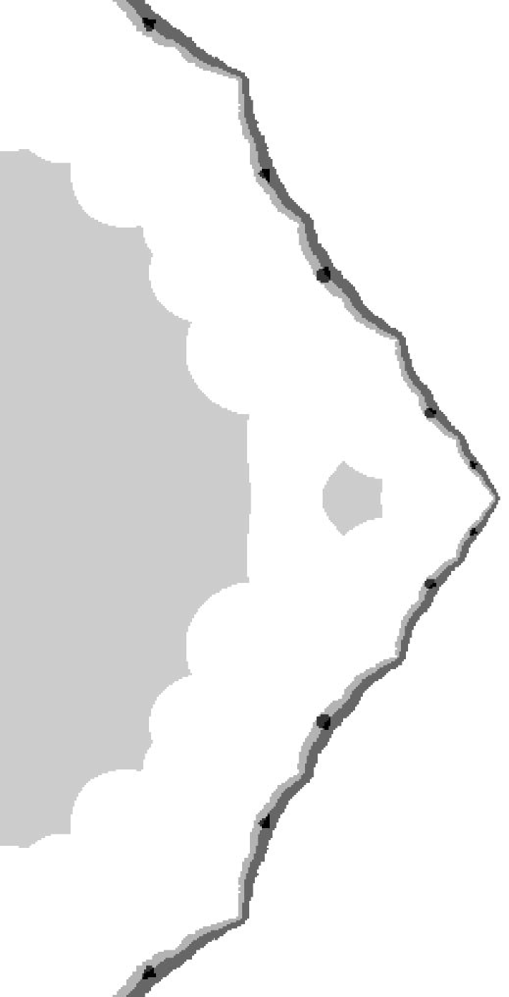
Figure 3. Shown above is the unstable manifold parameterization for a saddle fixed point of $H_{a,c},$ with $c=-.3,a=.1$, intersected with three box models $\Gamma_{1},\Gamma_{2},\Gamma_{3}$, containing pseudo-recurrent dynamics of $H$. The two islands in the large interior on the left are in $\Gamma_{2}$, the model of the fixed sink. The right hand band is $\Gamma_{1}$, containing $J$. The lighter band on $\Gamma_{1}$ is approximately contained in $K^{+}$. The darkest spots overlapping $\Gamma_{1}$ show $\Gamma_{3}$, which contains pseudo-recurrence but no true recurrence. Thus $\Gamma_{3}$ would be eliminated for smaller box size. Here boxes are of side length $(2\times 1.43)/2^{7}=0.022$, and $\Gamma_{1}$ contains $32{,}000$ boxes. This $\Gamma_{1}$ is box hyperbolic.

Now assume we have obtained a model $\Gamma$ which appears to contain $J$ but no other recurrent dynamics. We outline below the Axis Metric Algorithm for verifying box hyperbolicity on $\Gamma$, then describe each step in detail.

Algorithm 5.1 (Axis Metric Algorithm).

1. Define an approximately invariant splitting; specifically, a pair of “unstable” and “stable” vectors, $\mathbf{u}_{k},\mathbf{s}_{k}$, for each box, $B_{k}\in\mathcal{V}(\Gamma)$.

2. Build an “unstable” metric which is (approximately) uniformly expanded by $DH$ on the set of unstable directions, $\{\mathbb{C}\mathbf{u}_{k}\}$, and a “stable” metric which is (approximately) uniformly expanded by $DH^{-1}$ on the set of stable directions, $\{\mathbb{C}\mathbf{s}_{k}\}$.

3. Use the directions and their metrics to define the cones as Hermitian forms.

4. Finally, check whether $H$ preserves the cone field, and whether with respect to the Hermitian forms, $DH\ (DH^{-1})$ is expanding on the unstable (stable) cones.

In this algorithm, we will need to move around on the graph $\Gamma$ using the following:

Definition 5.2.

A directed graph $\Gamma_{0}$ is an arborescence if there is a root vertex $v_{0}$ so that for any other vertex $v$, there is a unique simple path from $v_{0}$ to $v$. Such a graph is a tree, and must have exactly one incoming edge for each vertex $v\neq v_{0}$.

If $\Gamma$ is strongly connected, then for each vertex $v_{0}$ in $\Gamma$, there is a minimum spanning tree $\Gamma_{0}$ with root vertex $v_{0}$ which is an arborescence (simply perform a depth first or breadth first search from $v_{0}$). We call such a $\Gamma_{0}$ a spanning arborescence. (See [10] for a discussion of implementation of basic graph theory).

Step 1 (Setting stable and unstable directions).

Recall from Section 2.2, that when $\left\lvert a\right\rvert\neq 1$, except on the curve of equation $4c=(1+a)^{2}$, the map $H_{a,c}$ has at least one saddle fixed point, $p$. If $H$ has no saddle fixed point, it should be possible to instead use a saddle periodic point of period greater than one, but this was not necessary for any of the maps we were interested in studying. The Hénon mapping $(x,y)\to(x^{2}+c-ay,x)$ has two fixed points. Note first that fixed points of $H$ must be on the diagonal, i.e., $x=y$. Then the two fixed points are:

$$x_{\pm}=\frac{1}{2}\left((1+a)\pm\sqrt{(1+a)^{2}+4c}\right).$$

By substituting the IA Hull of $a$ and $c$ into the above formula, and performing operations in IA, we compute $x_{\pm}$ as complex intervals (interval vectors in $\mathbb{R}^{2}$) containing the actual fixed points. Next, the eigenvalues of $D_{x}H$ for the fixed point $(x,x)$ are:

$$\lambda,\mu=x\pm\sqrt{x^{2}-a}.$$

Thus we test to see whether each interval vector $x_{\pm}$ is a saddle, by computing two real intervals containing the moduli of the eigenvalues, and then testing whether one interval is entirely greater than one, while the other is entirely less than one. So now assume $H$ has a saddle fixed point $p=(x,x)$. Bedford and Smillie have shown $J$ contains all saddle periodic points, hence $p\in J$, thus there is a box, $B_{0}$, in $\Gamma$, containing $p$. Let $\mathbf{u_{0}}\ (\mathbf{s_{0}})$ be the eigenvector of unit length corresponding to the unstable (stable) eigenvalue. These are natural unstable and stable directions in the box $B_{0}$. Since we will just use the $\mathbf{u_{k}}$’s and $\mathbf{s_{k}}$’s as axes for cones, we need only know them approximately, so here interval arithmetic is not needed.

Now let $\Gamma_{0}$ be a spanning arborescence of $\Gamma$, with root vertex $B_{0}$. To define unstable directions in each box $B_{k}$, sucessively push $\mathbf{u_{0}}$ across the edges of $\Gamma_{0}$ by $DH$. To be precise, fix a point $z_{k}$ in $B_{k}$, say the center point of the box, and for each edge $(k,j)\in\mathcal{E}({\Gamma_{0}})$, starting with $k=0$, define

$$\mathbf{u}_{j}:=\frac{D_{z_{k}}H(\mathbf{u}_{k})}{\|D_{z_{k}}H(\mathbf{u}_{k})\|}.$$

As noted above, we need only an approximation to the $\mathbf{u_{k}}$’s, so interval arithmetic is not used here. In fact, were we to attempt to use IA, we may encounter a computational difficulty. This is due to the recursive definition of the $\mathbf{u_{k}}$’s. Suppose we desired to compute “more” of the potential unstable directions in each box, by starting with an interval vector $\mathbf{U_{0}}$ in $\mathbb{C}^{2}$ guaranteed to contain the unstable eigenvector of $D_{p}H$, and then pushing this interval vector across $\Gamma_{0}$ to define interval vectors $\mathbf{U_{k}}$ in each box $B_{k}$. More precisely, a box $B$ is an interval vector in $\mathbb{C}^{2}$, so $B=(X,Y)$, with $X,Y$ complex intervals (interval vectors in $\mathbb{R}^{2}=\mathbb{C})$. Then

$$D_{p}H=\left[\begin{array}[]{rr}2p&-a\\ 1&0\end{array}\right]\text{ and }D_{B}H=\left[\begin{array}[]{rr}2X&-\text{Hull}(a)\\ \text{Hull}(1)&\text{Hull}(0)\end{array}\right],$$

so $D_{B}H$ has entries complex intervals. Then $D_{B_{k}}H(\mathbf{U_{k}})$ is an interval vector. Suppose $(1,2,\ldots,n)$ is a path in $\Gamma_{0}$ (this should be $(k_{1},\ldots,k_{n})$, but we wish to avoid too many nested subscripts). Then $\mathbf{U_{n}}=D_{B_{n}}H\circ\cdots\circ D_{B_{1}}H(\mathbf{U_{1}}).$ However, since the $B_{k}$’s are near $J$, due to the dynamical properties of $H$ on $J$, this type of iteration will (in experiment, very quickly) lead to intervals $\mathbf{U_{n}}$ to huge to be useful.

Define the stable directions similarly, keeping in mind that stable cones should be expanded and preserved by $DH^{-1}$. The transpose of a graph $\Gamma$, $\Gamma^{T}$, is the graph formed by reversing the edge directions of $\Gamma$. Thus to define $\mathbf{s}_{k}$, we use a spanning tree $\overline{\Gamma_{0}}$ of $\Gamma^{T}$ with $B_{0}$ as root vertex (note that $\overline{\Gamma_{0}}\neq\Gamma_{0}^{T}$), and push $\mathbf{s}_{0}$ across successive edges of $\overline{\Gamma_{0}}$ by $DH^{-1}$. Specifically, if $(j,k)\in\mathcal{E}({\overline{\Gamma_{0}}})$, then

$$\mathbf{s}_{k}=\frac{D_{z_{k}}H^{-1}(\mathbf{s}_{j})}{\|D_{z_{k}}H^{-1}(\mathbf{s}_{j})\|},$$

where $z_{k}\in B_{k}$ as in the definition of $\mathbf{u}_{k}$.

Proposition 5.3.

Let $\{\mathbf{u}_{k}\},\{\mathbf{s}_{k}\}$ be unstable and stable directions for each box $B_{k}$ of $\Gamma$, defined as above.

1. Let ${C}^{u}_{k}$ be any box constant cone field preserved by $D_{z}H$, for each $z\in B_{k}$. Then for each $B_{k}$, we must have $\mathbf{u}_{k}\subset{C}^{u}_{k}$.

2. Let ${C}^{s}_{k}$ be any box constant cone field preserved by $D_{z}H^{-1}$, for each $z\in B_{k}$. Then for each $B_{k}$, we must have $\mathbf{s}_{k}\subset{C}^{s}_{k}$.

Note that for edges $(k,m)$ in $\Gamma$ but not in the spanning arborescence $\Gamma_{0}$, $DH$ does not map $\mathbf{u}_{k}$ into $\mathbb{C}\mathbf{u}_{m}$. It is helpful in establishing invariance of the cone field if $DH(\mathbf{u}_{k})$ is close to $\mathbb{C}\mathbf{u}_{m}$, and in addition, if $D_{z}H$ does not vary greatly as ${z}$ varies within one box.

Thus before performing the next step, we take some measurements on the separation of the stable and unstable directions in each box, to get an idea of whether it might be possible to prove box hyperbolicity using these directions, and store (for later scrutiny) which boxes might be obstructions. In order to measure the difference between directions, we view a direction in $\mathbb{C}^{2}$ as a complex line in $\mathbb{C}^{2}$, and thus use the spherical metric, $\sigma$. Then, for each box $B_{k}$ in $\mathcal{V}(\Gamma)$, let

$$\text{Udiam}[k] = \text{diam}_{\sigma}\{D_{z_{j}}H(\mathbf{u_{j}})\colon(j,k)\in\mathcal{E}(\Gamma)\},\text{ and}$$

$$\text{Sdiam}[k] = \text{diam}_{\sigma}\{[D_{z_{k}}H]^{-1}(\mathbf{s_{j}})\colon(k,j)\in\mathcal{E}(\Gamma)\}.$$

We do not measure the variation within one box, i.e., between $D_{z}H$ and $D_{z_{k}}H$ for different $z$ in box $B_{k}$, since it seems that would be much smaller than among images from different boxes.

Proposition 5.3 suggests that a clear separation between Udiam$[k]$ and Sdiam$[k]$ is needed in order for a computer program to verify cone preservation under $DH$, thus we will not confidently progress to the next step unless we have

$$\sigma(\mathbf{u}_{k},\mathbf{s}_{k})-(\text{Udiam}[k]+\text{Sdiam}[k])>0$$

in each box $B_{k}$. Finally, we record in which boxes the either Udiam or Sdiam is large, or $\sigma-(\text{Udiam}+\text{Sdiam})$ is negative.

Step 2 (Building a metric on the directions).

Consider the unstable directions $\{\mathbb{C}\mathbf{u}_{k}\}_{k=1}^{N}$. As discussed above, $DH$ does not quite preserve these directions, so first we take that into account. Let $P^{\mathbf{u}}_{\mathbf{s}}$ be the projection onto $\mathbb{C}\mathbf{u}$ with $\mathbb{C}\mathbf{s}$ as its Null space. Given the vectors $\mathbf{u}=(u_{1},u_{2})$ and $\mathbf{s}=(s_{1},s_{2})$ in $\mathbb{C}^{2}$, this projection is:

$$P^{\mathbf{u}}_{\mathbf{s}}\genfrac{[}{]}{0.0pt}{}{v_{1}}{v_{2}}=\frac{v_{1}s_{2}-v_{2}s_{1}}{u_{1}s_{2}-u_{2}s_{1}}\genfrac{[}{]}{0.0pt}{}{u_{1}}{u_{2}}.$$

Then for each edge $(k,j)\in\mathcal{E}(\Gamma)$, we have $P^{\mathbf{u}_{j}}_{\mathbf{s}_{j}}\circ D_{z_{k}}H$ maps $\mathbb{C}\mathbf{u}_{k}$ to $\mathbb{C}\mathbf{u_{j}}$. If the unstable directions are a good approximation to an invariant unstable line field, then $P^{\mathbf{u}}_{\mathbf{s}}\circ DH$ is close to $DH$ on these unstable directions.

In [19], we describe a method for proving hyperbolicity of polynomial maps of one complex variable, by building a metric for which the map is expanding by some $L>1$ on a neighborhood of the Julia set. The neighborhood of $J$ is a collection of boxes in $\mathbb{C}$, and the metric in each box is defined by a constant times the $L^{\infty}$ metric in $\mathbb{R}^{2}=\mathbb{C}$. Say $\varphi_{k}\left\|\cdot\right\|$ is the metric on box $B_{k}$, then the constants $\varphi_{k}$ are called metric handicaps.

In two variables, we use this same algorithm twice: once for the unstable directions and once for the stable directions. For example, for the unstable direction field, we will attempt to build a metric for which $P^{\mathbf{u}}_{\mathbf{s}}\circ DH$ is box expansive by some amount $L>1$. This metric will be defined in each unstable direction $\mathbb{C}\mathbf{u_{k}}$ by a constant times our $L^{\infty}$ metric in $\mathbb{R}^{4}=\mathbb{C}^{2}$, say $\varphi^{u}_{k}\left\|\cdot\right\|$. Following the algorithm in [19], we call the $\varphi^{u}_{k}$ unstable metric handicaps, and define $\varphi^{u}_{0}=1$ in box $B_{0}$, then want to build handicaps satisfying

$$\varphi^{u}_{j}{\left\|P^{\mathbf{u}_{j}}_{\mathbf{s}_{j}}\circ D_{z_{k}}H(\mathbf{v})\right\|}\geq{L}\ \varphi^{u}_{k}\left\|\mathbf{v}\right\|,$$

for each edge $(k,j)\in\mathcal{E}(\Gamma)$, and each $\mathbf{v}\in\mathbb{C}\mathbf{u_{k}}$. But then $\mathbf{v}=\alpha\mathbf{u_{k}}$ for some $\alpha\in\mathbb{C}$, so since $P^{\mathbf{u}}_{\mathbf{s}}\circ DH$ is linear and $\left\|\mathbf{u}_{k}\right\|=1$, the above equation is equivalent to

(4) $$\varphi^{u}_{j}\geq\frac{L\ \varphi^{u}_{k}}{\left\|P^{\mathbf{u}_{j}}_{\mathbf{s}_{j}}\circ D_{z_{k}}H(\mathbf{u}_{k})\right\|}.$$

If we set $\xi_{k,j}=L/{\left\|P^{\mathbf{u}_{j}}_{\mathbf{s}_{j}}\circ D_{z_{k}}H(\mathbf{u}_{k})\right\|}$, then we can use Algorithm 4.4 of [19] to attempt to find metric handicaps satisfying $\varphi^{u}_{j}\geq\xi_{k,j}\varphi^{u}_{k}$, hence Equation 4, on each edge $(k,j)\in\Gamma$. This is of course not always possible, but the intuition is that it should be possible if the box model is sufficiently small in the right places. If it is not possible, then the user can try a smaller $L$, or start over with smaller boxes.

We use interval arithmetic in Equation 4 as in [19]. The $\varphi_{k}^{u}$’s will be chosen in $\mathbb{F}$ (machine knowable numbers, note $\varphi^{u}_{0}=1\in\mathbb{F}$). Then replace each number in the left hand side with it’s Hull (the smallest interval in $\mathbb{I}\mathbb{F}$ containing it). Then perform the operations in IA, and test whether the upper endpoint of the resulting interval is less than $\varphi^{u}_{j}$.

To attempt to define stable metric handicaps, use the method analogous to that for the unstable metric handicaps. That is, try to find an $M>1$ and build handicaps $\{\varphi^{s}_{k}\}$ so that

(5) $$\varphi^{s}_{j}\leq\frac{\varphi^{s}_{k}M}{\left\|P^{\mathbf{s}_{j}}_{\mathbf{u}_{j}}\circ D_{z_{k}}H(\mathbf{s}_{k})\right\|},$$

for each edge $(k,j)\in\mathcal{E}(\Gamma)$. Then the stable directions are box-contracted by $P^{\mathbf{s}}_{\mathbf{u}}\circ DH$. Again, if this step fails to produce a contracted metric, then the user can try a larger $M$, or start over with smaller boxes.

As we will see below, the ratio of stable to unstable metric handicaps in each box, $\varphi^{s}_{k}$ to $\varphi^{u}_{k}$, determines the width of the cones. Hence it is necessary to find values for $L$ and $M$ which yield comparable metrics. Lyapunov exponents give us some intuition. For a polynomial automorphism of $\mathbb{C}^{2}$, there are two Lyapunov exponents, $\lambda^{\pm}$, which measure expansion and contraction of tangent vectors. According to [7], if $f$ is a polynomial diffeomorphism of $\mathbb{C}^{2}$ with $d=d(f)>1$, then $\lambda^{+}\geq\log d$, $\lambda^{-}\leq-\log d$, and

(6) $$\lambda^{+}+\lambda^{-}=\log(\det Df).$$

Note that for Hénon mappings, ${\det(Df)}=a$. Thus $\lambda^{+}+\lambda^{-}=\log(a).$ Since $\lambda^{+}\geq\log d$, we have the inequality: $\lambda^{-}\leq\log(a)-\log d$. In the case $\left\lvert a\right\rvert<1$, we have $\log(a)<0$, hence the inequality for $\lambda^{-}$ is stronger than the inequality for $\lambda^{+}$. Thus in general we expect stronger contraction than expansion of tangent vectors under Hénon mappings. Equation 6 implies that a good rule of thumb for choosing $L$ and $M$ is $LM=\left\lvert a\right\rvert$. In practice, for any $\Gamma$ we tested, the algorithm for setting the stable metric handicaps given any $M$ always completed in much less time than the algorithm for setting unstable metric handicaps given an $L$ (perhaps due to the strong contraction). Thus after experimenting with various options, we have adopted the following strategy. First find the smallest working $M$ using simple bisection ($0<M<1$), then test expansion on the unstable directions using a value of $L$ near $\left\lvert a\right\rvert/M$.

In experiment we have observed that finding a working $L>1$ and $M<1$ is almost always possible when a box model $\Gamma$ has been found for $J$ which does not contain any sinks of $H$. Rather, the difficult step is the next one: checking whether the cone field defined by these metrics is preserved and expanded by $DH$.

Step 3 (Defining a cone field).

If Step 2 successfully constructed expanded and contracted metrics on the unstable and stable directions, respectively, then the metrics and directions always define cones in each box, as follows.

In each box, $B_{k}$, define the unstable cone, $C^{u}_{k}$, so that a vector $\mathbf{w}$ is in the unstable cone if it is closer to $\mathbf{u}_{k}$ than $\mathbf{s}_{k}$, relative to the unstable and stable metrics. That is, $\mathbf{w}\in C^{u}_{k}$ iff

$$\varphi^{u}_{k}\left\|P^{\mathbf{u}_{k}}_{\mathbf{s}_{k}}(\mathbf{w})\right\|\geq\varphi^{s}_{k}\left\|P^{\mathbf{s}_{k}}_{\mathbf{u}_{k}}(\mathbf{w})\right\|.$$

Then the stable cones are just the complements, $C^{s}_{k}:=\mathbb{C}^{2}\setminus C^{u}_{k}$.

We define the Hermitian form $Q_{k}\colon\mathbb{C}^{2}\to\mathbb{R}$, by

$$Q_{k}(\mathbf{w})=\left(\varphi^{u}_{k}\left\|P^{\mathbf{u}_{k}}_{\mathbf{s}_{k}}(\mathbf{w})\right\|\right)^{2}-\left(\varphi^{s}_{k}\left\|P^{\mathbf{s}_{k}}_{\mathbf{u}_{k}}(\mathbf{w})\right\|\right)^{2}.$$

Thus the unstable cone, $C^{u}_{k}$, is simply the set of vectors for which $Q_{k}$ is nonnegative, and the stable cone, $C^{s}_{k}$, is the set of vectors for which the form is negative.

We can construct a Hermitian matrix, $A_{k}$, which encodes the information of $Q_{k}$, following standard linear algebra as in [16]. A Hermitian form $Q$ defines a sesquilinear form $g\colon\mathbb{C}^{2}\times\mathbb{C}^{2}\to\mathbb{R}$, such that $g(\mathbf{w},\mathbf{w})=Q(\mathbf{w})$, where we can recover $g$ using:

$$g(\mathbf{v},\mathbf{w})=\frac{1}{4}Q(\mathbf{v}+\mathbf{w})-\frac{1}{4}Q(\mathbf{v}-\mathbf{w})+\frac{i}{4}Q(\mathbf{v}+i\mathbf{w})-\frac{i}{4}Q(\mathbf{v}-i\mathbf{w}).$$

A sesquilinear form $g$ can be represented by a matrix $A$ so that $g(\mathbf{v},\mathbf{w})=\mathbf{w^{*}}A\mathbf{v}$, with $a_{m,n}=g(\mathbf{e}_{n},\mathbf{e}_{m})$ for an ordered basis $\{\mathbf{e}_{1},\mathbf{e}_{2}\}$, like $\{(1,0),(0,1)\}$. Now $g$ Hermitian implies that $A$ is also Hermitian, and the range of $Q$ is $\mathbb{R}$. Thus, $Q(\mathbf{w})=\mathbf{w^{*}}A\mathbf{w}$, where $a_{m,n}=\frac{1}{4}Q(\mathbf{e}_{n}+\mathbf{e}_{m})-\frac{1}{4}Q(\mathbf{e}_{n}-\mathbf{e}_{m})+\frac{i}{4}Q(\mathbf{e}_{n}+i\mathbf{e}_{m})-\frac{i}{4}Q(\mathbf{e}_{n}-i\mathbf{e}_{m})$.

We easily calculate that for $\mathbf{u}=(u_{1},u_{2}),\mathbf{s}=(s_{1},s_{2})$, if we set

$$b_{11}=(\varphi^{u}\left\lvert s_{2}\right\rvert\left\|u\right\|)^{2}-(\varphi^{s}\left\lvert u_{2}\right\rvert\left\|s\right\|)^{2},\ \ b_{22}=(\varphi^{u}\left\lvert s_{1}\right\rvert\left\|u\right\|)^{2}-(\varphi^{s}\left\lvert u_{1}\right\rvert\left\|s\right\|)^{2},$$

$$b_{12} =\frac{1}{4} \left[(\varphi^{u}\left\|u\right\|)^{2}(\left\lvert s_{2}-s_{1}\right\rvert^{2}-\left\lvert s_{2}+s_{1}\right\rvert^{2}+i\left\lvert is_{2}-s_{1}\right\rvert^{2}-i\left\lvert is_{2}+s_{1}\right\rvert^{2})\right.$$

$$-\left.(\varphi^{s}\left\|s\right\|)^{2}(\left\lvert u_{2}-u_{1}\right\rvert^{2}-\left\lvert u_{2}+u_{1}\right\rvert^{2}+i\left\lvert iu_{2}-u_{1}\right\rvert^{2}-i\left\lvert iu_{2}+u_{1}\right\rvert^{2})\right],$$

and $b_{21}=\bar{b}_{12}$, then $a_{m,n}=b_{m,n}/{\left\lvert u_{1}s_{2}-u_{2}s_{1}\right\rvert^{2}}$.

In implementation, we use the above formulas to calculate, for each box $B_{k}$ in $\Gamma$, an interval valued matrix $A_{k}$, representing the form $Q_{k}$ defining the cone $C^{u}_{k}$. Note that since $A_{k}$ is Hermitian, the main diagonal entries are real intervals, and the other entries are (complex conjugate) complex intervals. As noted above, the vectors $\mathbf{u_{k}}$ and $\mathbf{s_{k}}$ and the handicaps $\varphi^{u}_{k},\varphi^{s}_{k}$ are chosen to be machine knowable numbers. Thus before the formulas defining $A_{k}$ are computed, these terms are converted to their interval Hulls, then the arithmetic operations are performed in IA to obtain $A_{k}$ with interval entries (of length greater than zero).

Remark 5.4.

Note that the ratio of the metric handicaps determines the angle width of the cones. Thus if $\varphi^{u}_{k}$ and $\varphi^{s}_{k}$ are several orders of magnitude different then the cones will be very thin, even if the unstable and stable directions are far apart, thus the cones will be difficult for the computer to work with. This is why it is necessary in Step 2 to find values of $L$ and $M$ which yield a comparable pair of metric handicaps in each box.

Step 4 (Checking whether cones are preserved and expanded).

For the last step of testing box hyperbolicity, we need to test whether $DH\ (DH^{-1}$) expands the unstable (stable) cones, with respect to $\{Q_{k}\}$. For this step we simply use Proposition 4.11, in which we showed that in order to get preservation and expansion of the unstable cones, and contraction of the stable cones, we need precisely that $((Q_{j}\circ D_{z}H)-Q_{k})$ is positive definite for every edge $(k,j)\in\mathcal{E}(\Gamma)$, and every $z\in B_{k}$. Thus in this step, we simply compute this form defined for each edge in the graph, and test whether it is positive definite.

In Step 3, for each box $B_{k}$ in $\Gamma$, we computed an interval matrix $A_{k}$ representing $Q_{k}$, in that $Q_{k}(\mathbf{w})=\mathbf{w}^{*}A_{k}\mathbf{w}$. Thus by Equation 3, the interval matrix representing $(Q_{j}\circ D_{z}H)-Q_{k}$ is

$$T_{k,j}=((D_{B_{k}}H)^{*}\ A_{j}\ D_{B_{k}}H)-A_{k}.$$

Using the formula for the interval matrix $D_{B_{k}}H$ from Step 1, it is straightforward to compute the interval matrix $T_{k,j}$. Now we need to check whether this matrix is positive definite. But since $T$ is Hermitian, the trace and determinant are real, and $T$ is positive definite iff its trace and determinant are positive (see [16]). The trace and determinant of $T$ are real intervals, so we simply compute them with IA and check whether their lower endpoints are positive.

If the above test succeeds (positive definite for each edge), then the model $\Gamma$ is box hyperbolic, hence $H$ is hyperbolic. If not, then we may record boxes which are obstructions, that is, boxes $B_{k},B_{j}$ for which $T_{k,j}$ fails to be positive definite.

This is the stopping point of the Axis Metric Algorithm for testing box hyperbolicity for a given $\Gamma$. If box hyperbolicity fails, the user may refine $\Gamma$ by choosing to subdivide either all the boxes, or some subset of the boxes which seem to be obstructing the hyperbolicity testing (for example, boxes marked in Steps 1 or 4 above), then test the new $\Gamma$ with the Axis Metric Algorithm. Two of the Hénon mappings of Theorem 1.3, $H_{a,c}$ with $(c,a)=(0,-.22)$ and $(1.5,.5)$, were proven hyperbolic for a model constructed by straight subdivision to a certain box size, then by subdividing twice only boxes marked in Step 4 (see next section).

6. Results of running Hypatia on Hénon mappings

Running Hypatia for a Hénon mapping is not quite as simple as inputting the parameters $a,c$ and awaiting the results, since the user must make decisions as to how to build the best $\Gamma$ for testing with the Axis Metric Algorithm. In this section, we describe the specific process we followed and results obtained for the mappings of Theorem 1.3.

Theorem 1.3 follows from Theorem 1.2, that box hyperbolicity of some $\Gamma$, a box chain model of $J$, implies hyperbolicity of $H$ on $J$, and from the fact that for each mapping mentioned in the theorem, using our computer program Hypatia, we constructed a box chain model of $J$ and verified box hyperbolicity with the Axis Metric Algorithm. Below, we discuss the process for each of these mappings in increasing order of the computational difficulty of proving hyperbolicity.

The quickest map to be proven hyperbolic was $H_{a,c},$ with $c=-.3,a=.1$. We simply used a box chain model of $J$ with boxes selected from an evenly subdivided $(2^{7})^{4}$ grid on $\mathcal{B_{0}}=[-1.43,1.43]^{4}$. Figure 3 shows the box hyperbolic $\Gamma$. This is a map seemingly in the main cardioid, with recurrent dynamics $J$ and a fixed sink.

For $H_{a,c},$ with $c=-3,a=-.25$, we also proved hyperbolic relatively quickly. The box chain model $\Gamma$ of $J$ from an evenly subdivided $(2^{7})^{4}$ grid on $B_{0}=[-2.57,2.57]^{4}$ is box hyperbolic. This mapping appears to be a real horseshoe (i.e., a horseshoe contained in $\mathbb{R}^{2}$). Figure 4 is a FractalAsm picture of the Julia set. This kind of picture is really the most useful for a Cantor set.

Figure 4. A FractalAsm picture of $W^{u}_{p}\cap K^{+}$ for $H_{a,c},$ with $c=-3,a=-.25$. This set appears to be a real Cantor set.

We proved the map $H_{a,c},$ with $c=0,a=-.22$, is hyperbolic by starting with a model of $J$ from an evenly subdivided $(2^{7})^{4}$ grid on $\mathcal{B}_{0}=[-R,R]^{4}$, for $R=1.32$, but then additionally performing three hyperbolicity tests, and each time subdividing only boxes in which the cone check of Step 4 of the Axis Metric Algorithm failed (to end with boxes of size ranging from $2R/2^{7}$ to $2R/2^{10}$). This map also seems to be in the main cardiod. The picture of the Julia set is similar to Figure 3.

Using nearly the same method as the previous mapping, we proved $H_{a,c},$ with $c=1.5,a=.5$, is hyperbolic. Here, we started with the even $(2^{8})^{4}$ grid on $\mathcal{B}_{0}=[-R,R]^{4}$, for $R=2.286$, then twice subdivided only boxes in which the cone check (Step 4 of the Axis Metric Algorithm) failed (yielding boxes of size $2R/2^{8}$ to $2R/2^{10}$). The resulting box chain model is box hyperbolic. FractalAsm pictures (see Figure 5) suggest this map is a complex horseshoe, with Julia set not contained in $\mathbb{R}^{2}$.

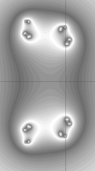
Figure 5. A FractalAsm picture of $W^{u}_{p}\cap K^{+}$ for $H_{a,c},$ with $c=1.5,a=.5$. This set appears to be a complex Cantor set. The origin of the axes is the saddle fixed point $p$.

Table 1 contains more data for all of the mappings discussed in this section. In the table, $\Gamma$ denotes the box chain model of $J$, for the map $H_{a,c}(x,y)=(x^{2}+c-ay,x)$. $R$ is the bound such that the boxes are contained in $\mathcal{B}_{0}=[-R,R]^{4}\subset\mathbb{R}^{4}=\mathbb{C}^{2}$. The box grid depth for a box is the number $n$ such that the box is of size $2R/2^{n}$. If a box chain model contains boxes of multiple sizes, then multiple box grid depths are listed.

Table 1. Data for the box chain models of Theorem 1.3. [*Data not collected.]

Figure		5	4	3	N/A
params.	$c$	$1.5$	$-3$	$-.3$	$0$
	$a$	$.5$	$-.25$	$.1$	$-.22$
sink period		N/A	N/A	$1$	$1$
$R$		$2.286$	$2.57$	$1.43$	$1.32$
box grid depth, $n$		$8$-$10$	$7$	$7$	$7$-$10$
box size		$0.018,0.009,0.0045$	$0.04$	$0.022$	$0.0052,0.0026,0.0013$
$\Gamma$ size ($1000$s)	boxes	$53$	$2.4$	$32$	$78$
	edges	$2{,}950$	$75$	$1{,}250$	$4{,}150$
$\sigma(\mathbf{u},\mathbf{s})$ (in $[0,\pi/2]$)	min.	*	$0.47$	$0.9$	*
	avg.	*	$1.15$	$1.07$	*
Udiam (in $[0,\pi/2]$)	max.	*	$0.13$	$0.015$	*
	avg.	*	$0.023$	$0.03$	*
Sdiam (in $[0,\pi/2]$)	max.	*	$0.11$	$0.0008$	*
	avg.	*	$0.01$	$0.0003$	*
$\sigma-(\text{Udiam}+\text{Sdiam})$	min.	*	$0.47$	$.09$	*
(in $[0,\pi/2]$)	avg.	*	$1.15$	$1.07$	*
$M$ (bisection)		$0.21680$	$0.111328$	$0.0596$	$0.140$
$L$ $(\approx\left\lvert a\right\rvert/M$)		$2.180$	$2$	$1.6789$	$1.480$
$\varphi^{s}_{k}$	min.	$0.0613$	$0.046$	$0.034$	$0.0425$
	max.	$1.079$	$1$	$1$	$1$
	avg.	$0.571$	$0.096$	$0.152$	$0.263$
$\varphi^{u}_{k}$ (in $(0,1]$)	min.	$0.046$	$0.033$	$0.072$	$0.0574$
	avg.	$0.268$	$0.09$	$0.158$	$0.177$
proved box-hyp?		YES	YES	YES	YES
runtime (min.)		$<10$	$<1$	$30$	$45$
RAM (MB)		$>250$	$20$	$220$	$1200$

References

- [1] Dynamics at Cornell. [http://www.math.cornell.edu/~dynamics].
- [2] E. Bedford, M. Lyubich, and J. Smillie. Distribution of periodic points of polynomial diffeomorphisms of . Invent. Math., 114(2):277–288, 1993.
- [3] E. Bedford, M. Lyubich, and J. Smillie. Polynomial diffeomorphisms of . IV. The measure of maximal entropy and laminar currents. Invent. Math., 112(1):77–125, 1993.
- [4] E. Bedford and J. Smillie. Real polynomial diffeomorphisms with maximal entropy: Tangencies. to appear, preprint available at [http://xxx.arxiv.org], arXiv:math.DS/0103038.
- [5] E. Bedford and J. Smillie. Polynomial diffeomorphisms of : currents, equilibrium measure and hyperbolicity. Invent. Math., 103(1):69–99, 1991.
- [6] E. Bedford and J. Smillie. Polynomial diffeomorphisms of . II. Stable manifolds and recurrence. J. Amer. Math. Soc., 4(4):657–679, 1991.
- [7] E. Bedford and J. Smillie. Polynomial diffeomorphisms of . VI. Connectivity of . Ann. of Math. (2), 148(2):695–735, 1998.
- [8] M. Benedicks and L. Carleson. The dynamics of the Hénon map. Ann. of Math. (2), 133(1):73–169, 1991.
- [9] Interval Computations. [http://www.cs.utep.edu/interval-comp/].
- [10] T. Cormen et al. Introduction to Algorithms. The MIT Electrical Engineering and Computer Science Series. The MIT Press and McGraw-Hill Book Company, 1990.
- [11] M. Dellnitz and O. Junge. Set oriented numerical methods for dynamical systems. In Handbook of dynamical systems, Vol. 2, pages 221–264. North-Holland, Amsterdam, 2002.
- [12] R. Devaney and Z. Nitecki. Shift automorphisms in the Hénon mapping. Comm. Math. Phys., 67(2):137–146, 1979.
- [13] M. Eidenschink. Exploring Global Dynamics: A Numerical Algorithm Based on the Conley Index Theory. PhD thesis, Georgia Institute of Technology, 1995.
- [14] J. E. Fornæss and N. Sibony. Complex Hénon mappings in and Fatou-Bieberbach domains. Duke Math. J., 65(2):345–380, 1992.
- [15] S. Friedland and J. Milnor. Dynamical properties of plane polynomial automorphisms. Ergodic Theory Dynamical Systems, 9(1):67–99, 1989.
- [16] K. Hoffman and R. Kunze. Linear Algebra Second Edition. Prentice Hall, 1971.
- [17] J. S. L. Hruska. On the numerical construction of hyperbolic structures for complex dynamical systems. PhD thesis, Cornell University, 2002. Download at [http://www.math.sunysb.edu/dynamics/theses/index.html].
- [18] S. L. Hruska. Rigorous numerical models for the dynamics of complex Hénon mappings on their chain recurrent sets. Discrete and Continuous Dynamical Systems, to appear. available at [http://xxx.arxiv.org].
- [19] S.L. Hruska. Constructing an expanding metric for dynamical systems in one complex variable. Nonlinearity, 18:81–100, 2005.
- [20] J. Hubbard and K. Papadantonakis. Exploring the parameter space of complex Hénon mappings. Journal of Experimental Mathematics, to appear.
- [21] J. Hubbard, P. Papadopol, and V. Veselov. A compactification of Hénon mappings in as dynamical systems. Acta Math., 184(2):203–270, 2000.
- [22] J. H. Hubbard and R. W. Oberste-Vorth. Hénon mappings in the complex domain. I. The global topology of dynamical space. Inst. Hautes Études Sci. Publ. Math., (79):5–46, 1994.
- [23] J. H. Hubbard and R. W. Oberste-Vorth. Hénon mappings in the complex domain. II. projective and inductive limits of polynomials. In B. Branner and P. Hjorth, editors, Real and Complex Dynamical Systems, volume 464 of NATO Adv. Sci. Inst. Ser. C Math. Phys. Sci., pages 89–132. Kluwer Acad. Publ., Dordrecht, 1995.
- [24] Y. Ishii and J. Smillie. On the hyperbolicity of some complex Hénon maps. in preparation.
- [25] K. Mischaikow. Topological techniques for efficient rigorous computations in dynamics. Acta Numerica, 2002.
- [26] R. E. Moore. Interval Analysis. Prentice-Hall, Englewood Cliffs, New Jersey, 1966.
- [27] R. E. Moore. Methods and Applications of Interval Analysis. SIAM Studies in Applied Mathematics, Philadelphia, 1979.
- [28] S. Morosawa, Y. Nishimura, M. Taniguchi, and T. Ueda. Holomorphic dynamics. Cambridge University Press, Cambridge, 2000. Translated from the 1995 Japanese original and revised by the authors.
- [29] S. Newhouse. Lectures on dynamical systems. In Dynamical Systems (C.I.M.E. Summer School, Bressanone, 1978), volume 8 of Progress in Mathematics, pages 1–114. Birkhäuser, Boston, Mass., 1980.
- [30] S. Newhouse and J. Palis. Bifurcations of Morse-Smale dynamical systems. In Dynamical systems (Proc. Sympos., Univ. Bahia, Salvador, 1971), pages 303–366. Academic Press, New York, 1973.
- [31] R. W. Oberste-Vorth. Complex horseshoes and the dynamics of mappings of two complex variables. PhD thesis, Cornell University, 1987.
- [32] R. Oliva. On the combinatorics of external rays in the dynamics of the complex Hénon map. PhD thesis, Cornell University, 1998.
- [33] G. Osipenko. Construction of attractors and filtrations. In Conley index theory (Warsaw, 1997), volume 47 of Banach Center Publ., pages 173–192. Polish Acad. Sci., Warsaw, 1999.
- [34] G. Osipenko and S. Campbell. Applied symbolic dynamics: attractors and filtrations. Discrete Contin. Dynam. Systems, 5(1):43–60, 1999.
- [35] PROFIL/BIAS Interval Arithmetic Package. [http://www.ti3.tu-harburg.de/Software/PROFILEnglisch.html].
- [36] C. Robinson. Dynamical systems. CRC Press, Boca Raton, FL, second edition, 1999. Stability, symbolic dynamics, and chaos.
- [37] W. Tucker. A rigorous ODE solver and Smale’s 14th problem. Found. Comput. Math., 2(1):53–117, 2002.