Rigorous numerical models
for the dynamics of complex Hénon mappings
on their chain recurrent sets

Suzanne Lynch Hruska

Department of Mathematics

Indiana University

Rawles Hall

Bloomington, IN 47405, USA

Abstract. We describe a rigorous and efficient computer algorithm for building a model of the dynamics of a polynomial diffeomorphism of $\mathbb{C}^{{2}}$ on its chain recurrent set, $\mathcal{R}$, and for sorting points into approximate chain transitive components. Further, we give explicit estimates which quantify how well this algorithm approximates the chain recurrent set and distinguishes the chain transitive components. We also discuss our implementation for the family of Hénon mappings, $f_{a,c}(x,y)=(x^{2}+c-ay,x)$, into a computer program called Hypatia, and give several examples of running Hypatia on Hénon mappings.

1. Introduction

Computer work, especially computer graphics, has been an important tool of discovery in the field of dynamical systems. This paper is also concerned with the use of computers but it has a different goal. The goal of this paper is to rigorously establish some results on the location of the set of points where recurrent behavior takes place. We focus on the class of polynomial diffeomorphisms of $\mathbb{C}^{{2}}$, which includes the widely studied family of Hénon mappings, $f_{a,c}(x,y)=(x^{2}+c-ay,x)$.

We start by examining a rigorous and effective computer algorithm for building a model of the dynamics of a map, $f$, on its chain recurrent set, $\mathcal{R}$, and for sorting points into approximate chain transitive components. We call this algorithm the box chain construction. The same basic algorithm has been studied previously, in different settings. Osipenko and Campbell ([20, 21]) approximate the chain recurrent set for a homeomorphism of a smooth, real, compact manifold. Eidenschink ([8]) discusses a similar procedure for real flows. A philosophically related procedure is studied in [6, 7], but their case of interest is the attractor of a real map (rather than the chain recurrent set). [15] is a recent survey of this work. The focus in the previous body of work is to develop a very general procedure for rigorously approximating $\mathcal{R}$ for continuous maps or flows in $\mathbb{R}^{{n}}$.

In this paper, we restrict our attention to polynomial diffeomorphisms of $\mathbb{C}^{{2}}$, which allows us to adapt the box chain construction and its implementation to be more efficient. In addition, we establish estimates on the accuracy of our model. These are explicit estimates, involving only the inputs to the program, which quantify how closely our box chain construction approximates the chain recurrent set. This allows us to predict when an execution of the program will successfully separate the distinct chain transitive components. We contrast this with the work of Dellnitz and Hohmann ([6]), which gives results on the accuracy of the approximation in the case that the map is hyperbolic; however, their estimates involve constants of hyperbolicity, which they do not discuss how to calculate. Osipenko and Campbell ([21]) give approximation estimates, in terms of some of the inputs to the program as well as selected output, hence the accuracy of their approximation can only be measured after execution of the algorithm.

Our first result on accuracy of the box chain construction for polynomial diffeomorphisms of $\mathbb{C}^{{2}}$ can be paraphrased as follows.

Theorem 1.1.

Let $f$ be a polynomial diffeomorphism of $\mathbb{C}^{{2}}$ (of dynamical degree $d>1$). Suppose $\mathcal{B}_{0}$ is a closed box in $\mathbb{C}^{{2}}$ containing the $\delta^{\prime}_{0}$-chain recurrent set, $\mathcal{R}({{\delta}^{\prime}_{0}})$, for some $\delta^{\prime}_{0}>0$ (for example, take $\mathcal{B}_{0},$ and $\delta=\delta^{\prime}_{0}>0$ as in Proposition 2.6).

The box chain construction produces sequences of constants, $\{\delta_{n}\}$ and $\{\varepsilon_{n}\}$, directed graphs, $\{\Gamma_{n}\}$, and regions in $\mathbb{C}^{{2}}$, $\{\mathcal{B}_{n}\}$, for $n\geq 1$, such that

1. $\delta_{n}\ll\varepsilon_{n}$ and both $\varepsilon_{n}\downarrow 0$ and $\delta_{n}\downarrow 0$ as $n\to\infty$,

2. the vertex set of $\Gamma_{n}$ is a collection of closed boxes $\{B^{n}_{k}\}$ in $\mathbb{C}^{{2}}$, which have side length at most $\varepsilon_{n}$,

3. each $\mathcal{B}_{n}$ is the region in $\mathbb{C}^{{2}}$ defined by the union of the $B^{n}_{k}$,

4. $\{\mathcal{B}_{n}\}$ is nested, i.e., $\{\cdots\subset\mathcal{B}_{n}\subset\cdots\subset\mathcal{B}_{1}\subset\mathcal{B}_{0}\}$,

5. there is guaranteed to be an edge in $\Gamma_{n}$ from $B^{n}_{k}$ to $B^{n}_{j}$ if $f(B^{n}_{k})$ intersects a $\delta_{n}$-neighborhood of $B^{n}_{j}$, and

6. we can calculate explicit sequences $\{\varepsilon^{\prime}_{n}\}_{n=1}^{\infty}$ and $\{\delta^{\prime}_{n}\}_{n=1}^{\infty}$, and an explicit constant $C$, such that for every $n\geq 1$,

   1. $\varepsilon^{\prime}_{n}\downarrow 0$, in particular $\varepsilon_{n}<\varepsilon^{\prime}_{n}\leq\delta_{n}+C\varepsilon_{n}$,

   2. $\delta^{\prime}_{n}$ is nonincreasing and converges to zero, with $\delta^{\prime}_{n}<\delta_{n}$, and

   3. $\mathcal{R}({{\delta}^{\prime}_{n}})\subset\mathcal{B}_{n}\subset\mathcal{R}({{\varepsilon}^{\prime}_{n}}).$

Definition 1.2.

For any $n\geq 1$, suppose $(\varepsilon,\delta,\Gamma,\mathcal{B})=(\varepsilon_{n},\delta_{n},\Gamma_{n},\mathcal{B}_{n})$ are produced by the box chain construction at step $n$, and satisfy Theorem 1.1.

We call the region $\mathcal{B}$ an $(\varepsilon,\delta)$-box chain recurrent set, and the graph $\Gamma$ an $(\varepsilon,\delta)$-box chain recurrent model of $f$. Each edge-connected component $\Gamma^{\prime}$ of $\Gamma$ is called an $(\varepsilon,\delta)$-box chain transitive component.

Conclusions (1) through (5) of Theorem 1.1 follow immediately from the description of the box chain construction, given in Section 2.2. Conclusion (6) is our first significant a priori estimate on the accuracy of our model, and is established in Sections 2.3 through 2.6. There we show that for the case of Hénon mappings, for any chosen $R^{\prime}>\left[1+\left\lvert a\right\rvert+\sqrt{(1+\left\lvert a\right\rvert)^{2}+4\left\lvert c\right\rvert}\right]/2,$ we get

$$\delta^{\prime}_{0} = \left[(R^{\prime})^{2}-(1+\left\lvert a\right\rvert)R^{\prime}-\left\lvert c\right\rvert\right]/2,$$

$$\delta^{\prime}_{n} = \min\left(\delta^{\prime}_{0},\ \left[-(2R^{\prime}+\left\lvert a\right\rvert+1)+\sqrt{(2R^{\prime}+\left\lvert a\right\rvert+1)^{2}+4\delta_{n}}\right]\right),and$$

$$\varepsilon^{\prime}_{n} = \delta_{n}+\varepsilon_{n}(1+\left\lvert a\right\rvert+2R^{\prime})+\varepsilon_{n}^{2}.$$

A box chain recurrent model of $f$ satisfies the definition of a symbolic image of $f$, given by Osipenko in [19]. Osipenko and Campbell ([21]) derive similar estimates to (6), but their version of $\varepsilon^{\prime}_{n}$ depends on measuring the size of the images of boxes $B_{k}$, after they have been computed.

We have implemented our efficient box chain construction for Hénon mappings into a computer program we call Hypatia. Using Hypatia we have produced many examples of box chain recurrent models of Hénon mappings. The box chain construction also has an immediate analog for polynomial maps of $\mathbb{C}$, which we include in Hypatia for quadratic and cubic polynomials. We keep the arithmetical computations in Hypatia rigorous using interval arithmetic with directed rounding. This method was recommended to us by Warwick Tucker, who used it in his recent computer proof that the Lorenz differential equation has the conjectured geometry ([24]). See Appendix B for a brief introduction to interval arithmetic.

The examples we are most interested in studying with Hypatia are Hénon mappings which are hyperbolic. These are the class of maps which have the “simplest” chaotic dynamics, and are in fact stable under small perturbation. Thus hyperbolic maps are the most amenable to rigorous computer investigation. In fact, Bedford and Smillie ([3]) have shown that for hyperbolic polynomial diffeomorphisms of $\mathbb{C}^{{2}}$, the chain recurrent set is well-behaved, in that it consists of simply the Julia set together with finitely many attracting or repelling periodic points.

The simplest hyperbolic Hénon mappings can be described in terms of the dynamics of some quadratic polynomial. In fact, if $f_{a,c}$ is a Hénon mapping with $a$ sufficiently small and $c$ is such that the polynomial $P_{c}(z)=z^{2}+c$ is hyperbolic, then $f|_{J}$ is topologically conjugate to the function induced by $P$ on the inverse limit ${\lim_{\leftarrow}(J,P)}$ ([14]). In this case, we say that $f$ is described by $P$, or simply that $f$ exhibits one dimensional behavior. The work of Hubbard and Papadontonakis ([13, 1]), and more specifically the work of Oliva ([18]), suggests points in parameter space which are conjectured to be hyperbolic and to have interesting properties. At the moment though neither the hyperbolicity nor the interesting properties have been established rigorously.

Thus a significant problem in the study of the Hénon family is to understand which maps exhibit one dimensional behavior, and to describe the behavior of maps which do not. Motivated by this problem, in this paper we use the box chain construction and its implementation in Hypatia to build box chain recurrent models for several interesting examples of Hénon mappings. Further, we use the results of this paper as the first step in a study of the property of hyperbolicity for polynomial diffeomorphisms of $\mathbb{C}^{{2}}$ in [11], and in a study of hyperbolicity (i.e., expansion) for polynomial maps of $\mathbb{C}$ in [12]. [10] contains an earlier version of the work of this paper, as well as that of [11, 12].

Example 1.3.

One of the simplest Hénon mappings which appears not to exhibit one dimensional behavior is $f_{a,c}$ with $(a,c)=(.125,-1.24)$. Oliva ([18]) gave combinatorial evidence that this diffeomorphism is hyperbolic with a period two attracting cycle, but is not described by a quadratic polynomial. Using our program Hypatia, we applied the box chain construction to the nearby map $(a,c)=(.15,-1.1875)$, which seems to be topologically conjugate to $(a,c)=(.125,-1.24)$. We computed a sequence terminating at a box chain recurrent set $\mathcal{B}_{8}$.

For a qualitative estimation of the accuracy of a box chain recurrent set, $\mathcal{B}$, we can sketch the intersection of $\mathcal{B}$ with a dynamically significant one-dimensional submanifold of $\mathbb{C}^{{2}}$: the unstable manifold of a saddle fixed point, which has a natural parameterization by $\mathbb{C}$. This process is explained in Appendix A.3 and Section 5.2. In Figure 1 we use this procedure to illustrate two box chain recurrent sets, $\mathcal{B}_{7}$ and $\mathcal{B}_{8}$, for the Hénon mapping with $(a,c)=(.15,-1.1875)$.

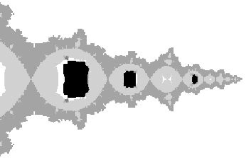
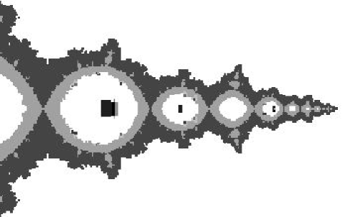
Figure 1. For $f_{a,c}$ the Hénon mapping with $c=-1.1875,a=.15$, $\mathcal{R}$ appears to be $J$ and a period $2$ sink. Shown in this figure are two box chain recurrent sets, restricted to the unstable manifold of a saddle fixed point, with its natural parameterization. On the top, boxes are of side length $2R/2^{6}$ and $2R/2^{7}$, where $R=1.9$. On the bottom is a refinement obtained from subdividing once some of the boxes on the top. The innermost, darkest regions in these figures are contained in the box chain transitive component containing the 2-cycle. Each box chain transitive component containing $J$ is shaded two tones by a heuristic algorithm, in order to illustrate how close the component is to $J$. The top is the crudest box chain recurrent model which separates $J$ from the sink. In the bottom figure, the small dark spots skirting the inner circles of the neighborhood of $J$ form a box chain transitive component of points which are pseudorecurrent but not recurrent.

Assuming the conjectural dynamics holds, the box chain recurrent models constructed for Example 1.3 are both successful in the sense of the following.

Definition 1.4.

Let $f$ be a polynomial diffeomorphism of $\mathbb{C}^{{2}}$ (of dynamical degree $d>1$). Let $\Gamma$ be a box chain recurrent model of $f$. We call $\Gamma$ separating if there are two chain transitive components, $\mathcal{R}^{j}$ and $\mathcal{R}^{k}$ (of $\mathcal{R}$), which lie in different box chain transitive components of $\Gamma$. In this case we say $\Gamma$ separates $\mathcal{R}^{j}$ and $\mathcal{R}^{k}$.

Further, we call $\Gamma$ fully separating if it separates every pair of chain transitive components.

Example 1.5.

Another interesting example studied by Oliva ([18]) is the Hénon mapping $f_{a,c}$ with $(a,c)=(.3,-1.17)$. We call this the 3-1-map, because it appears to be hyperbolic, with $\mathcal{R}$ consisting of three chain transitive components: $J$, an attracting fixed point, and an attracting cycle of period three. In contrast, quadratic polynomials cannot have more than one attracting cycle, thus this map appears not to exhibit one dimensional behavior. We applied the box chain construction to the 3-1-map, but were surprised to be unable to obtain a separating box chain recurrent model. The best box chain recurrent set we obtained is shown in Figure 2, intersected with the parameterized unstable manifold of a saddle fixed point.

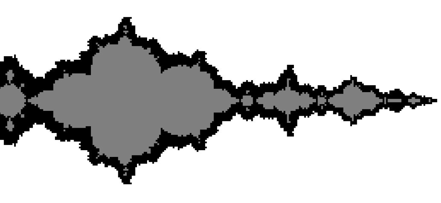
Figure 2. A box chain recurrent set for the Hénon mapping $f_{a,c},$ with $a=.3,c=-1.17$, restricted to the unstable manifold of a saddle fixed point, with its natural parameterization. Here boxes are of side length between $2R/2^{7}$ and $2R/2^{8}$, where $R=2.01$. Lighter gray points were heuristically found to be in $K^{+}$. Unfortunately, this box chain recurrent model does not separate $J$ from either the fixed sink or the attracting three-cycle.

Our difficulties with the 3-1-map motivated the following theorem, in which we calculate explicit bounds on $\varepsilon$ and $\delta$ to guarantee that an $(\varepsilon,\delta)$-box chain recurrent model will separate the fixed sink from the $3$-cycle and the Julia set. This gives a theoretical quantification of the computational difficulty of studying the 3-1-map.

Theorem 1.6.

Suppose $f_{a,c}$ is a Hénon mapping with an attracting fixed point $p$, with $\lambda_{1}\neq\lambda_{2}$ eigenvalues of $D_{p}f$, and $\lambda=\max(\left\lvert\lambda_{1}\right\rvert,\left\lvert\lambda_{2}\right\rvert)$. Set

$$\tau=\frac{\left\lvert\lambda_{1}-\lambda_{2}\right\rvert^{2}}{(2+\left\lvert\lambda_{1}\right\rvert+\left\lvert\lambda_{2}\right\rvert)(2+\lambda^{2}+\left\lvert a\right\rvert)}.$$

Let $\Gamma$ be an $(\varepsilon,\delta$)-box chain recurrent model of $f$. Let $M>1$ satisfy $\delta<\varepsilon/M$. Set

$$\kappa=\left[1+1/M+\max\{1,(1-\lambda)\sqrt{\tau}+2\left\|p\right\|+\left\lvert a\right\rvert\}\right].$$

If $\varepsilon<\frac{1}{2}\left(-\kappa+\sqrt{\kappa^{2}+\tau(1-\lambda)^{2}}\right),$ then $\Gamma$ separates the fixed sink from every other chain transitive component of $\mathcal{R}$.

This theorem applied to the 3-1-map yields that boxes of side length less than $4\times 10^{-5}$ would guarantee separation. However this is several orders of magnitude smaller than current resources allowed us to achieve with Hypatia. This demonstrates the need for the development of a more sophisticated construction for rigorously approximating chain recurrent sets of complex Hénon mappings.

Finally, we outline the remaining sections. In Section 2 we describe the box chain construction for polynomial diffeomorphisms of $\mathbb{C}^{{2}}$, and prove Theorem 1.1 by calculating explicit estimates on how well a box chain recurrent set approximates the chain recurrent set. In Section 3 we use some dynamical information about the map to develop two enhancements to the basic construction, significantly improving computational efficiency. In Section 4 we show a theoretical limitation of the box chain construction by proving Theorem 1.6, and applying the estimates of the theorem to the 3-1-map. In Section 5 we discuss examples generated with Hypatia, for Hénon mappings and a polynomial map of $\mathbb{C}$. We have included relevent background material on the chain recurrent set and the dynamics of Hénon mappings in Appendix A. In Appendix B we sketch the basics of interval arithmetic.

Acknowledgements. We thank John Smillie for providing guidance on this project, John Hubbard, Greg Buzzard, and Warwick Tucker for many helpful conversations on the topic, James Yorke, John Milnor, and Eric Bedford for advice on the preparation of this paper, Robert Terrell for technical support, and Michael Benedicks for pointing out to us that [15] describes a procedure similar to ours.

2. The box chain construction for polynomial diffeomorphisms of $\mathbb{C}^{{2}}$

In this section we start by giving an outline of the box chain construction, then discuss how we carry it out for polynomial diffeomorphisms of $\mathbb{C}^{{2}}$, to calculate the estimates leading to Theorem 1.1. To calculate our estimates, we assume a polynomial diffeomorphism of $\mathbb{C}^{{2}}$ (of dynamical degree $d(f)>1$) is a finite composition of generalized Hénon mappings, which are maps of the form $f(x,y)=(p(x)-ay,x)$, for $p$ monic of degree greater than one (see Appendix A).

2.1. Efficient neighborhoods

Before we begin our theoretical calculations, we want to specify that we do not use the euclidean metric. It is more natural for computer calculations to consider vectors in $\mathbb{R}^{{2n}}$, rather than $\mathbb{C}^{{n}}$, and use the $L^{\infty}$ metric, rather than euclidean. Thus throughout this paper, $\left\|\cdot\right\|$ will denote the $L^{\infty}$ norm on $\mathbb{R}^{{2n}}$, so that for a vector $x=(x_{1},\ldots,x_{n})\in\mathbb{C}^{{n}}$,

$$\left\|x\right\|=\max\{\left\lvert\text{Re}(x_{k})\right\rvert,\left\lvert\text{Im}(x_{k})\right\rvert\colon 1\leq k\leq n\}.$$

Also, let ${\mathcal{N}({S},{r})}$ denote the open $r$-neighborhood about the set $S$ in the metric $d_{\infty}$ induced by $\left\|\cdot\right\|$, e.g.,

$${\mathcal{N}({0},{r})}=\{x=(x_{1},\ldots,x_{n})\in\mathbb{C}^{{n}}\colon\left\lvert\text{Re}(x_{k})\right\rvert<r\text{ and }\left\lvert\text{Im}(x_{k})\right\rvert<r\}.$$

We use the simpler notation $\left\lvert\cdot\right\rvert$ for dimension $n=1$. This metric is uniformly equivalent to the euclidean metric on $\mathbb{C}^{{n}},\left\|\cdot\right\|_{e}$, since $\frac{1}{\sqrt{2n}}\left\|x\right\|_{e}\leq\left\|x\right\|\leq\left\|x\right\|_{e}.$ Neighborhoods are slightly different with respect to two uniformly equivalent norms, but the topology generated by them is exactly the same, thus they can practically be used interchangeably. Similarly, the $\varepsilon$-chain recurrent set $\mathcal{R}({\varepsilon})$ depends on choice of metric, but since $\mathcal{R}^{e}({\varepsilon})\subset\mathcal{R}({\varepsilon})\subset\mathcal{R}^{e}({\sqrt{2n}\varepsilon})$, the chain recurrent set $\mathcal{R}=\cap_{\varepsilon>0}\mathcal{R}({\varepsilon})$ is the same for any metric uniformly equivalent to euclidean. Thus throughout we use $\mathcal{R}({\varepsilon})$ as defined by our norm.

Remark 2.1.

When we say box, we mean a ball around a point in this norm. Note a box is also a vector of intervals, so boxes are neighborhoods which are easily manipulated with interval arithmetic.

2.2. The box chain construction

As suggested by the statement of Theorem 1.1, the box chain construction is an inductive process. We use the idea that any $\mathcal{R}({\varepsilon})$ consists of precisely the $\varepsilon$-pseudoperiodic orbits. Below is an outline of the basic construction.

We start with a polynomial diffeomorphism $f$ of $\mathbb{C}^{{2}}$ (of dynamical degree $d(f)>1$), and let $F$ be any interval extension of $f$, i.e., $F$ is a function on interval vectors such that for any box $B$, the image $F(B)$ is a box containing $f(B)$ (see Appendix B for background on interval arithmetic).

1. Given $f$ and an interval extension $F$, choose a small constant $\delta^{\prime}_{0}>0$, and a closed box $\mathcal{B}_{0}$ in $\mathbb{C}^{{2}}$ which contains $\mathcal{R}({{\delta}^{\prime}_{0}})$ (of $f$). Let $\varepsilon_{0}$ be the side length of the box $\mathcal{B}_{0}$. Choose $\delta_{0}$ such that $\varepsilon_{0}\gg\delta_{0}>\delta^{\prime}_{0}$.

2. Let $n\geq 0$. Suppose $\mathcal{B}_{n}$ is a closed region in $\mathbb{C}^{{2}}$, consisting of a collection of boxes $\mathcal{V}_{n}=\{B^{n}_{k}\}$ of side length at most $\varepsilon_{n}$, and such that $\mathcal{B}_{n}\supset\mathcal{R}({{\delta}^{\prime}_{n}})$, for some $\delta^{\prime}_{n}>0$. Suppose $\delta_{n}>\delta^{\prime}_{n}$ is given (if $n\geq 1$, then $\delta_{n}$ is given by step ($n-1$)-(ii).)

   1. Equally subdivide the boxes in $\mathcal{V}_{n}$. That is, choose $m>1$, set $\varepsilon_{n+1}=\varepsilon_{n}/m$, and place a grid of $m^{4}$ boxes inside each box of $\mathcal{V}_{n}$. This defines a new collection, $\mathcal{W}_{n+1}$, in which each box has side length $\varepsilon_{n+1}$.

   2. Build a graph approximating the map $f$ on $\mathcal{W}_{n+1}$. Specifically, choose some $\delta_{n+1}$ such that $\delta_{n+1}<\delta_{n}/2$ and $\delta_{n+1}\ll\varepsilon_{n+1}$ (for example, for every $n\geq 0$, set $\delta_{n}=\varepsilon_{n}/1000$). Then compute a directed graph $\Upsilon_{n+1}$ whose vertices are the boxes in $\mathcal{W}_{n+1}$, and such that there is guaranteed to be an edge from box $B^{n+1}_{k}$ to box $B^{n+1}_{j}$ if $F(B^{n+1}_{k})$ intersects a $\delta_{n+1}$-neighborhood of $B^{n+1}_{j}$.

   3. Find the subgraph of $\Upsilon_{n+1}$ consisting precisely of the vertices and edges which lie in cycles. Call this subgraph $\Gamma_{n+1}$. Let $\mathcal{V}_{n+1}=\{B^{n+1}_{k}\}$ be the vertices of $\Gamma_{n+1}$, and define $\mathcal{B}_{n+1}$ as the union of the boxes in $\mathcal{V}_{n+1}$.

Remark 2.2.

The box chain construction immediately implies that statements (1) through (5) of Theorem 1.1 are satisfied.

Remark 2.3.

The only difference between this basic box chain construction and the procedure used by Osipenko (and others as discussed in the introduction) is the presence of the constants $\delta^{\prime}_{n}$ and $\delta_{n}$. In order to approximating $\mathcal{R}$, these constants are uneeded, and can all be taken to be zero. However, in order to apply this construction to the problem of proving hyperbolicity, as we do in [12, 11], positive $\delta$’s are essential.

The first step in verifying the usefulness of this construction is to show that if $\mathcal{B}_{n-1}\supset\mathcal{R}({{\delta}^{\prime}_{n-1}})$, then there exists a $\delta^{\prime}_{n}$ such that $\mathcal{B}_{n}\supset\mathcal{R}({{\delta}^{\prime}_{n}})$. This fact for polynomial diffeomorphisms of $\mathbb{C}^{{2}}$ follows from Theorem 2.15 and Theorem 1.1, proved at the end of this section.

2.3. Trapping Regions for $\mathcal{R}$

In order to apply the box chain construction to polynomial diffeomorphisms of $\mathbb{C}^{{2}}$, we must first provide the base case, i.e., step (0) above. For this we prove Proposition 2.6, in which we calculate an explicit trapping region $\mathcal{B}_{0}$ for the $\delta$-chain recurrent set of polynomial diffeomophisms of $\mathbb{C}^{{2}}$. In particular, given a map $f$ and $\delta>0$, we give explicit $R^{\prime}$ such that $\mathcal{R}({{\delta}})\subset\mathcal{B}_{0}=\{\left\lvert x\right\rvert\leq R^{\prime},\left\lvert y\right\rvert\leq R^{\prime}\}$.

First we quantify how, for polynomial diffeomorphisms of $\mathbb{C}^{{2}}$, infinity in the $x$ direction is attracting, while infinity in the $y$ direction is repelling for $f$, and vice-versa for $f^{-1}$. A version of the following lemma is given in [9] (also see [23]).

Lemma 2.4.

Let $f$ be a polynomial diffeomorphism of $\mathbb{C}^{{2}}$, with $d(f)>1$. Let $\delta>0$. Then there is an $R>1$ and an $R^{\prime}>R$, such that if $\left\lvert x\right\rvert\geq R^{\prime}$ and $\left\lvert x\right\rvert\geq\left\lvert y\right\rvert$, then $\left\|f(x,y)\right\|\geq\left\lvert x\right\rvert+2\delta$.

If $f_{a,c}$ is a Hénon mapping, then $R=\frac{1}{2}(1+\left\lvert a\right\rvert+\sqrt{(1+\left\lvert a\right\rvert)^{2}+4\left\lvert c\right\rvert})$ and $2\delta=(R^{\prime})^{2}-(1+\left\lvert a\right\rvert)R^{\prime}-\left\lvert c\right\rvert$.

Proof.

Assume $f$ is a generalized Hénon mapping, $f(x,y)=(z,x)=(p(x)-ay,x)$, with $d=$deg$(p)>1$. So $p(x)=x^{d}+c_{d-1}x^{d-1}+\cdots+c_{0}$. Let $q(r)=r^{d}-\left\lvert c_{d-1}\right\rvert r^{d-1}-\cdots-\left\lvert c_{0}\right\rvert-(1+\left\lvert a\right\rvert)r$. Then there is an $R>0$ such that $q$ is monotone increasing on $[R,\infty)$, with $q(R)=0$. Note if $r>0$, then $q(r)\leq r^{d}-r$, thus $R\geq 1$.

Since $q$ is a polynomial and is monotone increasing on $[R,\infty)$, with $q(R)=0$, we see $q:(R,\infty)\to(0,\infty)$ is invertible. Thus given $\delta$, define $R^{\prime}\in(R,\infty)$ by $q(R^{\prime})=2\delta$.

Let $(x,y)\in\mathbb{C}$ satisfy $\left\lvert x\right\rvert\geq R^{\prime}$ and $\left\lvert x\right\rvert\geq\left\lvert y\right\rvert$. Then

$$\left\lvert z\right\rvert\geq\left\lvert p(x)\right\rvert-\left\lvert a\right\rvert\left\lvert y\right\rvert\geq\left\lvert p(x)\right\rvert-\left\lvert a\right\rvert\left\lvert x\right\rvert\geq q(\left\lvert x\right\rvert)+\left\lvert x\right\rvert\geq 2\delta+\left\lvert x\right\rvert.$$

If $f=f_{m}\circ\cdots\circ f_{1}$, then each composition moves $\left\lvert z\right\rvert$ farther away from $\left\lvert x\right\rvert$ additively. Thus, let $R^{\prime}_{k}$ satisfy $q_{k}(R^{\prime}_{k})=2\delta/m$ and take $R^{\prime}=\max\{R_{k}\}$, for $1\leq k\leq m$.

Note if $f_{a,c}$ is a quadratic Hénon mapping, $f_{a,c}(x,y)=(x^{2}+c-ay,x)$, then $q(r)=r^{2}-\left\lvert c\right\rvert+(1+\left\lvert a\right\rvert)r$, hence we easily achieve the claimed bound. ∎

Definition 2.5.

Let $\delta>0$. Following [2], we define the “trapping regions”, for $R^{\prime}\$ given by Lemma 2.4, by:

$$\mathcal{B}_{0} = \{\left\lvert x\right\rvert\leq R^{\prime}\text{ and }\left\lvert y\right\rvert\leq R^{\prime}\};$$

$$\mathcal{B}_{0}^{-} = \{\left\lvert x\right\rvert>R^{\prime}\text{ and }\left\lvert x\right\rvert>\left\lvert y\right\rvert\};$$

$$\mathcal{B}_{0}^{+} = \{\left\lvert y\right\rvert>R^{\prime}\text{ and }\left\lvert y\right\rvert>\left\lvert x\right\rvert\}.$$

Note the regions $\mathcal{B}_{0}=\mathcal{B}_{0}(\delta)$ depend on $\delta$, but in each instance the $\delta$ will be clear from context, so we will rarely use the notation $\mathcal{B}_{0}(\delta)$, rather we simply use $\mathcal{B}_{0}$.

The sets $V,V^{\pm}$ introduced in [2] are equal to $\mathcal{B}_{0},\mathcal{B}_{0}^{\pm}$ for $\delta=0$, and satisfy $K^{+}\subset V\cup V^{+},\ \ K^{-}\subset V\cup V^{-},\ \text{ and }K\subset V$ ([2]). Choosing $R^{\prime}$ larger than $R$ allows us to preserve these relationships and trap $\delta$-pseudo-orbits as well.

Proposition 2.6.

Let $f$ be a polynomial diffeomorphism of $\mathbb{C}^{{2}}$, with $d(f)>1$. Let $\delta>0$ and let $\mathcal{B}_{0}$ be as in Definition 2.5. Then $\mathcal{R}({{\delta}})\subset\mathcal{B}_{0}.$

Proof.

Given Lemma 2.4, we have $f(\mathcal{B}_{0}^{-})\subset\mathcal{B}_{0}^{-}$ and $f(\mathcal{B}_{0}^{-})\cap\mathcal{N}({\mathcal{B}_{0}},{2\delta})=\emptyset$. Thus if $p\in\mathcal{B}_{0}^{-}$, then $p$ is not in $\mathcal{R}({{\delta}})$, since the images $f(x_{k})$ move by at least $2\delta$ in the $x$ direction, and so the $x_{k+1}$ coming back in by only $\delta$ makes it impossible for $x_{n}=p$.

Similarly, for $p\in\mathcal{B}_{0}^{+}$ look at the chain backwards to contradict $\delta$-chain recurrence. ∎

To get an idea of the size of $R$, note that $R=2$ for $c=2$. Since the Mandelbrot set is contained in $\{x:\left\lvert x\right\rvert\leq 2\}$, for the parameters we tend to study we have $1\leq R\leq 2$. For a Hénon mapping, the values of $R$ are also close to this range.

2.4. Defining the graphs $\Upsilon$ and $\Gamma$

In steps (ii) and (iii) of the box chain construction, we compute graphs $\Upsilon$ and $\Gamma$ representing the action of $f$ (or $F$) on our collection of boxes. The following terminology will ease our discussion of these graphs.

About notation: if $\Gamma$ is a graph, then $\mathcal{V}(\Gamma)$ denotes the vertex set of $\Gamma$, and $\mathcal{E}(\Gamma)$ denotes its edge set. Also we often discuss one subset of a collection of boxes $\mathcal{V}=\{B_{k}\}_{k=1}^{N}$ at a time, and since the ordering is unimportant we avoid double subscripts and simply use $\{B_{0},B_{1},\ldots,B_{\ell}\}$.

Definition 2.7.

Let $\Upsilon=\Upsilon_{n}$ be the directed graph built in step (n)-(ii) of a box chain construction. Then we say $\Upsilon$ is an $(\varepsilon,\delta)$-box chain model of $F$.

In addition, when we say $\Upsilon$ is an $(\varepsilon,\delta)$-box chain model of $f$, we mean the “theoretically ideal” model, using the ideal interval extension of $f$, i.e., require $F(B_{k})=$ Hull$(f(B_{k}))$, for all boxes $B_{k}$.

Note for any interval extension $F$ of $f$, we know $F(B)\supset\text{Hull}(f(B))$ for any box $B$. Thus any result which is true for all interval extensions $F$ of $f$ is also true for $f$. Thus our default is to discuss box chain models of $F$, and only use box chain models of $f$ when trying to be precise about theoretical estimates.

Suppose $\Upsilon$ is an $(\varepsilon,\delta)$-box chain model of $F$. Note by Definition 1.2, the subgraph $\Gamma$ consisting of the cycles of $\Upsilon$ is called an $(\varepsilon,\delta)$-box chain recurrent model of $F$.

Remark 2.8.

Both a box chain model and a box chain recurrent model of $f$ satisfy the definition of a symbolic image of $f$, given by Osipenko in [19].

When the context is clear, or the distinction is unimportant, we simply refer to a box chain recurrent model as a box chain model. Thus we use the symbol $\Upsilon$ for any graph which is either a box chain model or a box chain recurrent model, and reserve $\Gamma$ for box chain recurrent models.

The following standard concept in graph theory will help us to analyze $\Gamma$.

Definition 2.9.

Let $\Upsilon$ be a directed graph. If there is a path from vertex $v$ to vertex $u$, then we say $u$ is reachable from $v$. A strongly connected component (SCC) is an equivalence class under the “are mutually reachable” equivalence relation. If an SCC consists of only one vertex, it must have an edge to itself.

Note the following easy relationship.

Lemma 2.10.

Let $\Upsilon$ be any directed graph. Let $\Gamma$ be the subgraph of $\Upsilon$ consisting of the vertices and edges which lie in cycles. Then $\Gamma=(\Gamma^{1}\sqcup\Gamma^{2}\sqcup\ldots\sqcup\Gamma^{l})$ is precisely the subgraph of $\Upsilon$ consisting of the union of the SCC’s of $\Upsilon$.

Recall from Definition 1.2 that the box chain transitive components of $\Gamma$ are defined as the edge-connected components of $\Gamma$, hence these are precisely the SCC’s of $\Upsilon$. The relationship between a box chain transitive component and an $\varepsilon$-chain transitive component is made precise in Corollary 2.17, and justifies our terminology. Thus the decomposition of a graph $\Gamma$ into its SCC’s is analogous to the partitioning of the chain recurrent set into it’s invariant pieces, the chain transitive components.

[5] gives a standard procedure for decomposing a graph into its SCC’s.

2.5. Estimates on $\Upsilon$ and $\Gamma$

Now we can calculate estimates which quantify our models. We begin with a lemma on the size of the image of the boxes.

Lemma 2.11.

Let $\Upsilon_{n}$ be an $(\varepsilon_{n},\delta_{n})$-box chain model of $f$. Then there exists $r_{n}>0$ (depending on $\varepsilon_{n}$, $f$, and $\mathcal{B}_{0}$) such that for $\varepsilon_{n}^{\prime}=(r_{n}+1)\varepsilon_{n}+\delta_{n}$, and for any $B_{k}\in\mathcal{V}({\Upsilon_{n}})$, we have:

1. the side length of the box $\text{Hull}(f(B_{k}))$ is less than or equal to $\varepsilon_{n}r_{n}$, and

2. if $(k,j)\in\mathcal{E}({\Upsilon_{n}})$, then for any $x_{k}\in B_{k}$ and any $x_{j}\in B_{j}$, $\left\|f(x_{k})-x_{j}\right\|<\varepsilon^{\prime}_{n}$.

For $f_{a,c}$ a Hénon mapping, we may take $r_{n}=\varepsilon_{n}+(2R^{\prime}+\left\lvert a\right\rvert)$, where $R^{\prime}$ is as in Proposition 2.6.

Proof.

The second item follows immediately from the first item, and the fact that if $B_{j}\cap\mathcal{N}({\text{Hull}(f(B_{k}))},{\delta})\neq\emptyset$, then there must be an edge from $B_{k}$ to $B_{j}$. We prove the first item using the linearization of $f$ to approximate it.

We assume $f$ is a generalized Hénon mapping, so $f(x,y)=(p(x)-ay,x)$, $p$ monic of degree $d>1$. Let $B\in\mathcal{V}({\Upsilon})$ and $(z,w)\in B$. The linearization of $f$ at $(z,w)$ is

$$L_{z}f(x,y)=f(z,w)+D_{z}f(x-z,y-w)=(p(z)-p^{\prime}(z)(x-z)-ay,x).$$

Note $L_{z}f(z,w)=f(z,w)$, for any $w$. Next, we observe

$$\left\|f(x,y)-L_{z}f(x,y)\right\|=\left\|(p(x)-p(z)-p^{\prime}(z)(x-z),0)\right\|\leq\sum_{k=2}^{d}\frac{\left\lvert p^{(k)}(z)\right\rvert}{k!}\left\lvert x-z\right\rvert^{k}.$$

If $(x,y)$ is also in $B$, then $\left\lvert x-z\right\rvert\leq\varepsilon_{n}$. Since $p$ is a polynomial, and $z\in\mathcal{B}_{0}=\mathcal{N}({0},{R^{\prime}})$, then for any $k\geq 0$, there exist $T_{k}\geq 0$ such that $\left\lvert p^{(k)}(z)\right\rvert/k!\leq T_{k}$. Hence,

$$\sum_{k=2}^{d}\frac{\left\lvert p^{(k)}(z)\right\rvert}{k!}\left\lvert x-z\right\rvert^{k}\leq\sum_{k=2}^{d}T_{k}\varepsilon_{n}^{k}.$$

Now we need to bound

$$\left\|L_{z}f(x,y)-L_{z}f(z,w)\right\|=\max\left(\left\lvert x-z\right\rvert,\left\lvert p^{\prime}(z)(x-z)-a(y-w)\right\rvert\right).$$

If $(x,y)$ is in $B$, then we also know $\left\lvert x-z\right\rvert\leq\varepsilon_{n}$, and

$$\left\lvert p^{\prime}(z)(x-z)-a(y-w)\right\rvert\leq T_{1}\varepsilon_{n}+\left\lvert a\right\rvert\varepsilon_{n}.$$

Finally, we put the above pieces together to compute, for any $(x,y),(z,w)$ in $B$,

$$\left\|f(x,y)-f(z,w)\right\|\leq\sum_{k=2}^{d}T_{k}\varepsilon_{n}^{k}+\varepsilon_{n}\max\left(1,T_{1}+\left\lvert a\right\rvert\right).$$

Hence, if $r_{n}$ is set to be the maximum above divided by $\varepsilon_{n}$, then we have that the diameter of the set $f(B_{k})$ in the metric $\left\|\cdot\right\|$ is less than or equal to $r_{n}\varepsilon_{n}$, hence the side length of Hull($f(B_{k})$) is less than or equal to $r_{n}\varepsilon_{n}$.

For $f_{k}$ a generalized Hénon mapping, we have $r_{n}(f_{k})$ as defined above. Now, if $f=f_{m}\circ\cdots\circ f_{1}$, then set $r_{n}=r_{n}(f_{1})\cdots r_{n}(f_{m})$. This suffices, for if we let $s(f_{k},\varepsilon)=r_{n}(f_{k})\varepsilon$ be the bound on the diameter of a box of size $\varepsilon$ under $f_{k}$, then we get $s_{1}=s(f_{1},\varepsilon_{n})=\varepsilon_{n}r_{n}(f_{1}),$ then $s_{2}=s(f_{2}\circ f_{1},\varepsilon_{n})=s(f_{2},s_{1})=s_{1}r_{n}(f_{2})=\varepsilon r_{n}(f_{1})r_{n}(f_{2}),$ etc., and $s_{m}=s(f_{m}\circ\cdots\circ f_{1})=s(f_{m},s_{m-1})=\varepsilon r_{n}(f_{1})\cdots r_{n}(f_{m}).$

In the case of $f_{a,c}$ a Hénon mapping, since $p(z)=z^{2}+c$ we can compute that $T_{1}=2R^{\prime}$ and $T_{2}=1$, and recall from Proposition 2.6, we have $R^{\prime}>1$. Hence $r_{n}=\varepsilon_{n}+\max\left(2R^{\prime}+\left\lvert a\right\rvert,1)=\varepsilon_{n}+(2R^{\prime}+\left\lvert a\right\rvert\right)$. ∎

This lemma give us the following component of Theorem 1.1.

Corollary 2.12.

Item (6)-(a) of Theorem 1.1 is satisifed.

Proof.

First, we show there exists a $C>0$ such that for any $n>1$, $r_{n}\leq C-1$, hence $\varepsilon^{\prime}_{n}\leq\delta_{n}+C\varepsilon_{n}$.

Suppose for all $n\geq 1$ that $\varepsilon_{n}<1$. Then we know $\varepsilon_{n}^{k}<\varepsilon_{n}$ for any $k>1$. Define $C=1+\sum_{k=2}^{d}T_{k}+\max\left(1,T_{1}+\left\lvert a\right\rvert\right)$ for a generalized Hénon mapping, or in the manner analogous to the previous proof for a composition (i.e., for $f=f_{m}\circ\cdots\circ f_{1}$, take $C=(C_{m}-1)\cdots(C_{1}-1)+1$). Then we see $r_{n}\leq C-1$.

On the other hand, since $\varepsilon_{n}$ is a decreasing sequence (see Remark 2.2), at most $\varepsilon_{n}>1$ for $0\leq n\leq N$. Thus if we set $C=1+\max\{r_{1},\ldots r_{N},\sum_{k=2}^{d}T_{k}+\max\left(1,T_{1}+\left\lvert a\right\rvert\right)\}$, then $r_{n}\leq C-1$ for all $n\geq 1$.

Finally, the above lemma defines $\varepsilon^{\prime}_{n}$ so that $\varepsilon^{\prime}_{n}>\varepsilon_{n}$. Hence we have $\varepsilon_{n}<\varepsilon^{\prime}_{n}\leq\delta_{n}+C\varepsilon_{n}$. By construction (see Remark 2.2) we know both $\varepsilon_{n}$ and $\delta_{n}$ decrease to zero as $n\to\infty$, hence $\varepsilon^{\prime}_{n}$ must as well. ∎

The next lemma will allow us to find $\delta^{\prime}$ for which a box chain recurrent model traps all $\delta^{\prime}$ pseudo-periodic orbits, i.e., $\mathcal{R}({{\delta}^{\prime}})$.

Lemma 2.13.

Let $\Upsilon_{n}$ be an $(\varepsilon_{n},\delta_{n})$-box chain model of $F$. There exists an $\eta=\eta(n)\in(0,\delta_{n})$, such that if $x\in\mathcal{N}({B_{k}},{\eta})$ and $f(x)\in\mathcal{N}({B_{j}},{\eta})$, then there is an edge from $B_{k}$ to $B_{j}$ in $\Upsilon_{n}$, i.e., $(k,j)\in\mathcal{E}({\Upsilon_{n}})$.

For $f_{a,c}$ a Hénon mapping, we can take

$$\eta(n)=\frac{1}{2}\left(-(2R^{\prime}+\left\lvert a\right\rvert+1)+\sqrt{(2R^{\prime}+\left\lvert a\right\rvert+1)^{2}+4\delta_{n}}\right),$$

where $R^{\prime}$ is as in Proposition 2.6.

Proof.

Again we give the proof for $f(x,y)=(p(x)-ay,x)$, $p$ monic of degree $d>1$. Let $(x,y)\in\mathcal{N}({B_{k}},{\eta})$ and $f(x,y)\in\mathcal{N}({B_{j}},{\eta})$. Let $(z,w)$ be a point in $B_{k}$ which realizes this minimum distance (since $B_{k}$ is closed), i.e., $\left\|(x,y)-(z,w)\right\|<\eta.$ Then in order to guarantee that $(k,j)\in\mathcal{E}({\Upsilon})$, we just need $\left\|f(x,y)-f(z,w)\right\|<\delta_{n}-\eta.$ But examining the proof of Lemma 2.11, since $(z,w)\in B_{k}$, we see that we have

$$\left\|f(x,y)-f(z,w)\right\|\leq\sum_{k=2}^{d}T_{k}\eta^{k}+\eta\max\left(1,T_{1}+\left\lvert a\right\rvert\right).$$

Thus, we just need $\eta$ to satisfy

$$\sum_{k=2}^{d}T_{k}\eta^{k}+\eta\left(\max\left(1,T_{1}+\left\lvert a\right\rvert\right)+1\right)-\delta_{n}<0.$$

Let $q_{n}(t)=\sum_{k=2}^{d}T_{k}t^{k}+t\max\left(2,T_{1}+\left\lvert a\right\rvert+1\right)-\delta_{n}$. Then we set $\eta=\eta(n)$ to be the smallest positive root of $q_{n}$. If $f=f_{m}\circ\cdots\circ f_{1}$, we may take $\eta=\min\{\eta(f_{1}),\ldots,\eta(f_{m})\}$. For $f_{a,c}$ a Hénon mapping, we get $q_{n}(t)=t^{2}+t(2R^{\prime}+\left\lvert a\right\rvert+1)-\delta_{n}$, which leads to the claimed bound. ∎

Corollary 2.14.

Recall $\mathcal{B}_{0}$ denotes the initial bounding box, with $\mathcal{R}({{\delta}^{\prime}_{0}})\subset\mathcal{B}_{0}$ for some $\delta^{\prime}_{0}>0$. For each $n\geq 1$, set $\delta^{\prime}_{n}=\min(\eta(n),\delta^{\prime}_{0})$, with $\eta(n)$ as in Lemma 2.13.

Then item (6)-(b) of Theorem 1.1 is satisfied.

Proof.

Lemma 2.13 states that $\eta(n)<\delta_{n}$, hence $\delta^{\prime}_{n}<\delta_{n}$. Next, note from the proof of Lemma 2.13 that $\eta$ is a monotone increasing function of $\delta_{n}>0$. By Remark 2.2 the sequence $\delta_{n}$ decreases as $n$ increases. Hence as $n$ increases, we get $\eta(n)$ decreases. Thus $\delta^{\prime}_{n}$ is at most equal to $\delta^{\prime}_{0}$ for a finite number of terms $N$, and then for $n>N$, $\delta^{\prime}_{n}$ decreases. ∎

2.6. Quantifying the accuracy of an $(\varepsilon,\delta)$-box chain recurrent set $\mathcal{B}$

In this section, we combine the lemmas of the previous section to achieve Theorem 2.15, which immediately implies Theorem 1.1 along with several relevant corollaries.

Theorem 2.15.

Suppose $\Upsilon_{n}$ is an $(\varepsilon_{n},\delta_{n})$-box chain model of $f$, and $\Gamma_{n}$ is the $(\varepsilon_{n},\delta_{n})$-box chain recurrent model of $f$ consisting of the SCC’s of $\Upsilon_{n}$. Let $\varepsilon^{\prime}_{n}$ be as in Lemma 2.11 and let $\delta^{\prime}_{n}$ be as in Corollary 2.14.

Let $\mathcal{B}(\Gamma_{n})=\mathcal{B}_{n}$ denote the region in $\mathbb{C}^{{2}}$ covered by the box vertices of $\Gamma_{n}$. Then item (6)-(c) of Theorem 1.1 is satisfied, i.e.,

$$\mathcal{R}({{\delta}^{\prime}_{n}})\subset\mathcal{B}(\Gamma_{n})\subset\mathcal{R}({{\varepsilon}^{\prime}_{n}}).$$

Proof.

We use the fact that precisely the vertices which lie in cycles in $\Upsilon_{n}$ are those which are in some strongly connected component of $\Upsilon_{n}$.

We handle the two inclusions separately. First consider the inclusion $\mathcal{R}({{\delta}^{\prime}_{n}})\subset\mathcal{B}(\Gamma_{n})$. We first need to establish $\mathcal{R}({{\delta}^{\prime}_{n}})\subset\mathcal{B}(\Upsilon_{n})$, which we prove by induction. For $n=0$, we can choose any $\delta^{\prime}_{0}>0$, and produce the box $\mathcal{B}_{0}$ such that $\mathcal{R}({{\delta}^{\prime}_{0}})\subset\mathcal{B}_{0}$ by Proposition 2.6. Consider $\Upsilon_{0}=\Gamma_{0}$ to be the graph with the single vertex $\mathcal{B}_{0}$ with an edge to itself. Now suppose $n\geq 1$, and assume $\mathcal{R}({{\delta}^{\prime}_{n-1}})\subset\mathcal{B}(\Gamma_{n-1})$. Observe that since the boxes of $\Upsilon_{n}$ are obtained from subdividing the boxes of $\Gamma_{n-1}$, we have $\mathcal{B}(\Upsilon_{n})=\mathcal{B}(\Gamma_{n-1})$, hence $\mathcal{R}({{\delta}^{\prime}_{n-1}})\subset\mathcal{B}(\Upsilon_{n})$. Also, since $\delta^{\prime}_{n}\leq\delta^{\prime}_{n-1}$ (Corollary 2.14) we have $\mathcal{R}({{\delta}^{\prime}_{n}})\subset\mathcal{R}({{\delta}^{\prime}_{n-1}})$. Thus $\mathcal{R}({{\delta}^{\prime}_{n}})\subset\mathcal{B}({\Upsilon_{n}})$.

Suppose $p\in\mathcal{R}({{\delta}^{\prime}_{n}})$. Then there exist $x_{1}=p,x_{2},\ldots,x_{m-1},x_{m}=p$ such that $\left\|f(x_{k})-x_{k+1}\right\|<\delta^{\prime}_{n}$ for $1\leq k<m$. Note that $x_{k}\in\mathcal{R}({{\delta}^{\prime}_{n}})$, for $1\leq k<m$. Hence each $x_{k}\in\mathcal{B}({\Upsilon_{n}})$ as well. Then there are boxes $B_{k}\in\Upsilon_{n}$ such that $x_{k}\in B_{k}$ for $1\leq k<m$. Since $\left\|f(x_{k})-x_{k+1}\right\|<\delta^{\prime}_{n}$, we have $f(x_{k})\in\mathcal{N}({B_{k+1}},{\delta^{\prime}_{n}})$. Since $\delta^{\prime}_{n}\leq\delta_{n}$, there is an edge in $\Upsilon_{n}$ from $B_{k}$ to $B_{k+1}$.

Hence, $p$ is in a box $B_{1}$ which lies in a cycle of $\Upsilon_{n}$, $B_{1}\to B_{2}\to\cdots\to B_{m-1}\to B_{1}$. Thus $B_{1}\in\mathcal{V}({\Gamma_{n}})$, hence $p\in\mathcal{B}_{n}$.

For the second inclusion, $\mathcal{B}(\Gamma_{n})\subset\mathcal{R}({{\varepsilon}^{\prime}_{n}})$, suppose $p\in\mathcal{B}(\Gamma_{n})$. Thus $p$ lies in some box $B_{1}$ which lies in a cycle $B_{1}\to B_{2}\to\cdots\to B_{m-1}\to B_{1}$ in $\Upsilon_{n}$. Recall $\varepsilon_{n}$ is the side length of the boxes in the graph $\Gamma_{n}$. Let $x_{1}=x_{m}=p$, and $x_{k}$ be any point in $B_{k}$ for $2\leq k\leq m-1$. Then by Lemma 2.11, since $B_{1}\to B_{2}\to\cdots B_{m-1}\to B_{1}$ is a cycle in $\Upsilon_{n}$, we have $\left\|f(x_{k})-x_{k+1}\right\|<\varepsilon^{\prime}_{n}$ for $1\leq k\leq m$. Hence, $p$ is $\varepsilon^{\prime}_{n}$-chain recurrent. ∎

Note this theorem completes the proof of Theorem 1.1.

A first modification of this theorem is that if we consider $\delta^{\prime}=0$ in the hypothesis, we can conclude $\mathcal{R}\subset\mathcal{B}_{n}\subset\mathcal{R}({\varepsilon^{\prime}})$. We need this observation in Section 3 to justify the process of eliminating “$\mathcal{B}_{0}$-escaping” boxes.

Next, extending from the theoretical $f$ to the practical $F$, we immediately obtain:

Corollary 2.16.

Suppose $\Upsilon_{n}$ is an $(\varepsilon_{n},\delta_{n})$-box chain model of $F$, and $\Gamma_{n},\varepsilon^{\prime}_{n},\delta^{\prime}_{n},$ and $\mathcal{B}_{n}$ are as in Theorem 2.15.

Let

$$s_{n}({F})=\sup_{B_{k}\in\mathcal{V}(\Gamma_{n})}\text{sidelength}[F(B_{k})-\text{Hull}(f(B_{k}))].$$

Then

$$\mathcal{R}({{\delta}^{\prime}_{n}})\subset\mathcal{B}_{n}\subset\mathcal{R}(\varepsilon^{\prime}_{n}+s_{n}(F)).$$

We cannot compute $s_{n}(F)$ exactly, but simply strive to design an implementation to minimize it. We shall not discuss that matter in detail in this paper, but refer the reader to the interval arithmetic resources listed in Section B. Away from the boundaries of machine precision, it is reasonable to assume $s_{n}(F)$ decreases as $\varepsilon_{n}$ decreases, and that $s_{n}(F)$ is small compared to $\varepsilon^{\prime}_{n}$. In fact, for a naive interval extension of $f$, $s_{n}(F)=O(\varepsilon_{n})$.

We can also immediately apply the theorem to the SCC’s.

Corollary 2.17.

Assume the hypothesis of Theorem 2.15.

1. Let $\mathcal{R}^{\prime}({{\delta}^{\prime}})$ be any $\delta^{\prime}$-chain transitive component. Then there is a box chain transitive component, $\Gamma^{\prime}$, such that $\mathcal{R}^{\prime}({{\delta}^{\prime}})\subset\mathcal{B}({\Gamma^{\prime}})$.

2. Let ${\Gamma^{\prime}}$ be any box chain transitive component of $\Gamma$. Then there is some $\varepsilon^{\prime}$-chain transitive component, $\mathcal{R}^{\prime}({{\varepsilon^{\prime}}})$, such that $\mathcal{B}({\Gamma^{\prime}})\subset\mathcal{R}^{\prime}({{\varepsilon^{\prime}}})$.

Again, in Corollary 2.17 with the weaker hypothesis $\delta^{\prime}=0$, we can form a conclusion analogous to (1) by setting $\delta^{\prime}=0$, i.e., $\mathcal{R}({{\delta}^{\prime}})=\mathcal{R}$.

Note that more than one $\delta^{\prime}$-chain transitive component can be contained in a single box chain transitive component. Also, an $\varepsilon^{\prime}$-chain component may not actually contain any chain recurrent points, hence a strongly connected component may not contain any chain recurrent points. We explore this further in Section 4.

For polynomial diffeomorphisms of $\mathbb{C}^{{2}}$ (with $d(f)>1)$, the Julia set $J$ is contained in a single chain transitive component $\mathcal{R}^{\prime}$ of $\mathcal{R}$ (see Theorem A.1). Hence Corollary 2.17 implies:

Corollary 2.18.

Assume the hypothesis of Theorem 2.15. Then there is a single box chain transitive component ${\Gamma^{\prime}}$ such that $J\subset\mathcal{B}({\Gamma^{\prime}})$.

Thus, one of the box chain transitive components, $\Gamma^{\prime}$, contains $J$. The others either contain attracting (or repelling) periodic orbits, or do not intersect $\mathcal{R}$. We can easily identify the component containing $J$, for it has by far the most vertices.

Remark 2.19.

Note the box chain construction and all of the estimates and results of this section can be reformulated to apply to polynomial maps of $\mathbb{C}$ of degree $d>1$, by simply dropping the $y$-component, and setting $a=0$ in all of the calculations. We use these results to study polynomial maps of $\mathbb{C}$ in [12].

See Section 5 for examples of box chain recurrent models generated with the program Hypatia.

3. Improving efficiency using Dynamics

One result of our interest in the complex case is that we are forced to deal with increased computational complexity difficulties, since working in $\mathbb{C}^{{2}}$ is the same for a computer as working in $\mathbb{R}^{4}$. In our experience, the main computational limitation is memory usage (even using a computer with 4 GB of RAM). Thus we keep memory efficiency in mind when tailoring the box chain construction to polynomial diffeomorphisms of $\mathbb{C}^{{2}}$. In this section, we discuss how to insert into the box chain construction two improvements, designed to increase efficiency, but without completely negating Theorem 2.15. In designing these algorithms, we take advantage of the dynamics of the map.

3.1. Step (i^′): Selective Subdivision

Note first that a single step (rather than inductive) construction consisting of simply subdividing the initial $\mathcal{B}_{0}$ into a very large grid of very small boxes is conceptually much simpler, but very computationally inefficient. In addition to the obvious work that subdivision saves, the tree structure it creates is useful for quickly computing things such as which boxes intersect a given set (like the image of another box). This allows us to store each graph as an array of vertices, with edges as adjacency lists, with no need to arrange the vertices in any particular order in the array. Further, the tree structure created by subdivision lends itself easily to be improved in the following manner.

In trying to approximate a dynamically defined set, it is natural to improve upon the basic subdivision procedure by replacing step (i) of the box chain construction with the more sophisticated selective subdivision procedure. The philosophy here is that we can concentrate our resources on the regions which are most “troublesome” by allowing boxes of different sizes. We would ideally define grid boxes so that the dynamical behavior in each box is varying by at most a small amount. Thus, we would like to refine down to a certain reasonable box size, then somehow select only a small fraction of the boxes to be subdivided further, leaving the rest unchanged.

1. Sort the boxes in $\mathcal{V}_{n}$ into two sets: $\mathcal{V}^{s}_{n}$ is boxes to be subdivided, and $\mathcal{V}^{u}_{n}$ is boxes to remain unchanged. Equally subdivide the boxes in $\mathcal{V}^{s}_{n}$: choose $m>1$ and place a grid of $m^{4}$ boxes inside each box of $\mathcal{V}^{s}_{n}$, to obtain the collection $\mathcal{W}^{s}_{n+1}$. Set $\mathcal{W}_{n+1}=\mathcal{W}^{s}_{n+1}\cup\mathcal{V}^{u}_{n}$. Then each box in $\mathcal{W}_{n+1}$ has side length at most $\varepsilon_{n+1}=\varepsilon_{n}$, and at least $\varepsilon_{n}/m$.

Note in this case the sequence of maximum box side lengths $\{\varepsilon_{n}\}$ is nonincreasing, rather than decreasing. In order to acheive the ideal accuracy in the limit, as in Theorem 2.15, one would have to subdivide all of the boxes once every few steps.

To implement this procedure, we must somehow choose which boxes to subdivide. A first goal is to obtain a box chain recurrent model which separates the Julia set from the attracting and repelling periodic orbits. With the goal of “refining out” the attracting behavior, we implemented in Hypatia an option to subdivide only boxes which seem to be in $K^{+}$. We call this sink basin subdivision. For example, one way of detecting boxes in sink basins is to choose boxes such that all eigenvalues of a few iterates of the derivative matrix $Df$ are small. In some cases, sink basin subdivision does help to separate out the sink dynamics more quickly (see Example 5.2). However, there are interesting examples for which this still does not allow us to separate the sink from $J$ (see Example 4.1). Thus, it seems that a selective subdivision procedure could be an extremely useful step, however it is unclear what are the optimal selection criteria for a given map.

3.2. Step (i.5): Eliminating $\mathcal{B}_{0}$-escaping boxes

After performing step (i) or (i^′), i.e., subdividing the desired level $n$ boxes $\mathcal{V}_{n}$ to obtain a new collection of level ${n+1}$ boxes, $\mathcal{W}_{n+1}$, but before performing step (ii) (i.e., computing a graph representing the action of $f$ (or $F$) on the collection of boxes), we institute an additional efficiency improving check: eliminating $\mathcal{B}_{0}$-escaping boxes. This is a very useful technique which removes much of the work of computing the graph in step (ii). The idea is to eliminate boxes whose images eventually lie outside of $\mathcal{B}_{0}$.

Note by examining the proof of Proposition 2.6 that if $f^{m}(B_{k})\cap\mathcal{B}_{0}=\emptyset$ for some $m>1$, then $B_{k}$ contains no points of $\mathcal{R}$. Thus we can delete vertex $k$ from the graph before computing the edge list. For the Hénon family, we can also take advantage of invertibility. That is, it follows from Lemma 2.4 that if $f^{-m}(B_{k})\subset\mathbb{C}\setminus\mathcal{B}_{0}$, then $B_{k}$ contains no points of $\mathcal{R}$. Thus we can check forward and backward images of boxes, deleting any boxes with some image leaving $\mathcal{B}_{0}$, and then in step (ii) compute the edge list for the reduced graph.

1. Given a collection of boxes $\mathcal{W}_{n+1}$, eliminate the $\mathcal{B}_{0}$-escaping boxes. Remaining is a subcollection of boxes $\mathcal{W}^{h}_{n+1}$ (which contains $\mathcal{R}$). Replace $\mathcal{W}_{n+1}$ with $\mathcal{W}^{h}_{n+1}$.

Each $\mathcal{B}_{n}$ in the constructed sequence contains $\mathcal{R}$, so we may call it an $(\varepsilon,0)$-approximation to $\mathcal{R}$. Such a sequence satisfies slightly weaker versions of Theorem 2.15 and Corollary 2.17, with ${\delta^{\prime}}$ replaced by $0$, and $\mathcal{R}({{\delta}^{\prime}})$ replaced by $\mathcal{R}$. Note however we still use the $\delta$ factor to build the edges in the graph, thus we still satisfy Lemma 2.11 and Lemma 2.13 (this is important in [12] and [11]).

In many instances, this check eliminates half or even three-fourths or more of the new boxes. Since the main computational limitation of Hypatia is in memory usage, not having to store edges corresponding to boxes which are eliminated with this iteration check is a big gain. Specific data for some examples is in Table 2, in Section 5.

4. Separating $J$ from a fixed sink

In this section, we calculate a theoretical limitation of the box chain construction in the case of a Hénon mapping, $f(x,y)=(x^{2}+c-ay,x)$, with an attracting fixed point $p=(z,z)$. In particular, we establish Theorem 1.6, quantifyiing a box size which guarantees that the box chain construction produces a box chain recurrent model separating the fixed sink from $J$, as in Definition 1.4, i.e., such that the fixed sink lies in a separate box chain transitive component from $J$. This quantification is in terms of $a,c$, and the eigenvalues, $\lambda_{1}\neq\lambda_{2}$, of $D_{p}f$, and $\lambda=\max(\left\lvert\lambda_{1}\right\rvert,\left\lvert\lambda_{2}\right\rvert)$.

First we find a euclidean disk contained in the sink basin, in Proposition 4.8. Second, we quantify an annular region about the sink which contains only non $\varepsilon$-chain recurrent points, in Proposition 4.11. We use this along with the estimates of Section 2 to derive Theorem 1.6. Finally, we apply our estimates to the 3-1-map.

Example 4.1 (The 3-1-map).

Recall from Example 1.5 that the Hénon mapping $f_{a,c}$ with $(a,c)=(.3,-1.17)$ is an interesting example because it appears to have two attracting periodic cycles, one of period three and one of period one. Two attracting cycles is not a phenomenon which can occur for the quadratic polynomial $f_{c}(z)=z^{2}+c$. Unfortunately, using our program Hypatia implementing the box chain construction, we failed to separate the sinks from $J$ before running out of the $4$ GB of RAM available on our computer.

In an attempt to find a good box chain recurrent set, we first uniformly subdivided all boxes to obtain a $(2^{7})^{4}$ grid on $\mathcal{B}_{0}=\mathcal{N}({0},{2.01})$, with box side length $2R/2^{7}=0.03$, where $R=2.01$. Then we used sink basin subdivision (Section 3), which subdivided about half of the boxes. At this point, the smallest boxes had side length $2R/2^{8}=0.015$. The box chain recurrent model $\Gamma$ was composed of $944{,}000$ boxes and $66{,}500{,}000$ edges. This used approximately $3.2$ GB of RAM, thus it seemed we could not subdivide significantly farther.

We also tried uniformly subdividing to obtain a $(2^{6})^{4}$ grid on $\mathcal{B}_{0}$, then invoking sink basin subdivision, twice, to get some boxes as small as above. However, this did not significantly decrease the amount of memory used.

Figure 2 shows the unstable manifold slice of the box chain recurrent set from the $(2^{7})^{4}$ grid on $\mathcal{B}_{0}$. We were initially surprised that we could not achieve separation for this map. This motivated the estimates of this section.

4.1. A dynamically significant norm

To quantify the dynamical notations of interest, we need to start with a metric which respects the dynamics.

Definition 4.2.

Note the Jacobian of $f$ is

$$D_{(x,y)}f=\begin{bmatrix}2x&-a\\ 1&0\end{bmatrix}$$

Suppose $\lambda_{1}\neq\lambda_{2}$ are the eigenvalues of $D_{p}f$, for the fixed sink $p=(z,z)$. Let $\lambda=\max(\left\lvert\lambda_{1}\right\rvert,\left\lvert\lambda_{2}\right\rvert)$. Note that since $p$ is a fixed sink, $\left\lvert\lambda\right\rvert<1$. Let $\{\mathbf{v_{1}},\mathbf{v_{2}}\}$ be the basis of eigenvectors, where we choose $\mathbf{v_{j}}=(\lambda_{j},1)$. Then $\mathbf{A}=[\mathbf{v_{1}}\ \mathbf{v_{2}}]$ is the change of basis matrix, i.e., if $\{\mathbf{e_{1}},\mathbf{e_{2}}\}$ is the standard basis in $\mathbb{C}^{{2}}$, then $\mathbf{A}\mathbf{e_{j}}=\mathbf{v_{j}}$. Let $\left\|\cdot\right\|_{e}$ be the euclidean norm in $\mathbb{C}^{{2}}$. Define the norm $\left\|\cdot\right\|_{\sigma}$ by $\left\|\mathbf{u}\right\|_{\sigma}:=\left\|\mathbf{A}^{-1}\mathbf{u}\right\|_{e}.$

We show below that $f$ is contracting with respect to $\left\|\cdot\right\|_{\sigma}$ in an neighborhood of $p$. First, we show this metric is uniformly equivalent to euclidean, and compute the constants of equivalence.

Lemma 4.3.

For all $\mathbf{u}\in\mathbb{C}^{{2}}$, $C\left\|\mathbf{u}\right\|_{\sigma}\leq\left\|\mathbf{u}\right\|_{e}\leq D\left\|\mathbf{u}\right\|_{\sigma},$ where $C,D$ are positive constants given by

$$C=\frac{\left\lvert\lambda_{1}-\lambda_{2}\right\rvert}{\sqrt{2+\left\lvert\lambda_{1}\right\rvert+\left\lvert\lambda_{2}\right\rvert}},\ \ \ \ D=\sqrt{2+\left\lvert a\right\rvert+\lambda^{2}}.$$

Proof.

Let $(x,y)$ be any vector in $\mathbb{C}^{{2}}$. To calculate both C and D, we use the following observation:

(1) $$0\leq(\left\lvert x\right\rvert-\left\lvert y\right\rvert)^{2}\text{ \ implies \ }2\left\lvert x\right\rvert\left\lvert y\right\rvert\leq\left\lvert x\right\rvert^{2}+\left\lvert y\right\rvert^{2}.$$

Recall $\left\|(x,y)\right\|_{\sigma}=\left\|\mathbf{A}^{-1}(x,y)\right\|_{e}.$ Since our eigenvectors are $\mathbf{v_{j}}=(\lambda_{j},1)$,

$$\mathbf{A}=\begin{bmatrix}\lambda_{1}&\lambda_{2}\\ 1&1\end{bmatrix},\text{ \ and \ }\mathbf{A}^{-1}=\frac{1}{\lambda_{1}-\lambda_{2}}\begin{bmatrix}1&-\lambda_{2}\\ -1&\lambda_{1}\end{bmatrix}.$$

First we show that we can set $C$ as claimed:

$$\left\lvert\lambda_{1}-\lambda_{2}\right\rvert^{2}\left\|(x,y)\right\|_{\sigma}^{2}=\left\lvert\lambda_{1}-\lambda_{2}\right\rvert^{2}\left\|\mathbf{A}^{-1}(x,y)\right\|_{e}=\left\lvert x-\lambda_{2}y\right\rvert^{2}+\left\lvert-x+\lambda_{1}y\right\rvert^{2}$$

$$\leq 2\left\lvert x\right\rvert^{2}+\left\lvert y\right\rvert^{2}(\left\lvert\lambda_{2}\right\rvert^{2}+\left\lvert\lambda_{1}\right\rvert^{2})+2\left\lvert x\right\rvert\left\lvert y\right\rvert(\left\lvert\lambda_{2}\right\rvert+\left\lvert\lambda_{1}\right\rvert),\text{ by triangle inequality},$$

$$\leq 2\left\lvert x\right\rvert^{2}+\left\lvert y\right\rvert^{2}(\left\lvert\lambda_{2}\right\rvert^{2}+\left\lvert\lambda_{1}\right\rvert^{2})+(\left\lvert x\right\rvert^{2}+\left\lvert y\right\rvert^{2})(\left\lvert\lambda_{2}\right\rvert+\left\lvert\lambda_{1}\right\rvert),\text{ by Equation~{}\ref{eqn:crossest}},$$

$$= \left\lvert x\right\rvert^{2}\left(2+\left\lvert\lambda_{1}\right\rvert+\left\lvert\lambda_{2}\right\rvert\right)+\left\lvert y\right\rvert^{2}\left(\left\lvert\lambda_{2}\right\rvert^{2}+\left\lvert\lambda_{1}\right\rvert^{2}+\left\lvert\lambda_{2}\right\rvert+\left\lvert\lambda_{1}\right\rvert\right),$$

$$\leq (\left\lvert x\right\rvert^{2}+\left\lvert y\right\rvert^{2})(2+\left\lvert\lambda_{1}\right\rvert+\left\lvert\lambda_{2}\right\rvert),\text{ since }\left\lvert\lambda_{1}\right\rvert,\left\lvert\lambda_{2}\right\rvert\leq 1,\text{ so }\left\lvert\lambda_{2}\right\rvert^{2}+\left\lvert\lambda_{1}\right\rvert^{2}\leq 2.$$

Next we need to establish that $\left\|\mathbf{u}\right\|_{e}\leq D\left\|\mathbf{u}\right\|_{\sigma}=D\left\|\mathbf{A}^{-1}\mathbf{u}\right\|_{e}$, for all $\mathbf{u}\in\mathbb{C}^{{2}}$. Since $\mathbf{A}$ is invertible, this is is equivalent to: $\left\|\mathbf{A}\mathbf{u}\right\|_{e}\leq D\left\|\mathbf{A}\mathbf{u}\right\|_{\sigma}=D\left\|\mathbf{u}\right\|_{e}$, for all $\mathbf{u}\in\mathbb{C}^{{2}}$. The following establishes this latter statement with $D$ as claimed:

$$\left\|\mathbf{A}(x,y)\right\|_{e}^{2}=\left\lvert\lambda_{1}x+\lambda_{2}y\right\rvert^{2}+\left\lvert x+y\right\rvert^{2},$$

$$\leq \left\lvert x\right\rvert^{2}(\left\lvert\lambda_{1}\right\rvert^{2}+1)+\left\lvert y\right\rvert^{2}(\left\lvert\lambda_{2}\right\rvert^{2}+1)+2\left\lvert x\right\rvert\left\lvert y\right\rvert(\left\lvert\lambda_{1}\right\rvert\left\lvert\lambda_{2}\right\rvert+1)\ \text{(triangle ineq.)},$$

$$\leq \left\lvert x\right\rvert^{2}\left(\left\lvert\lambda_{1}\right\rvert^{2}+\left\lvert\lambda_{1}\right\rvert\left\lvert\lambda_{2}\right\rvert+2\right)+\left\lvert y\right\rvert^{2}\left(\left\lvert\lambda_{2}\right\rvert^{2}+\left\lvert\lambda_{1}\right\rvert\left\lvert\lambda_{2}\right\rvert+2\right)\ \text{(Equation~{}\ref{eqn:crossest})},$$

$$\leq \left(\left\lvert x\right\rvert^{2}+\left\lvert y\right\rvert^{2}\right)\left(\lambda+\left\lvert\lambda_{1}\right\rvert\left\lvert\lambda_{2}\right\rvert+2\right),\text{ since we defined }\lambda=\max(\left\lvert\lambda_{1}\right\rvert,\left\lvert\lambda_{2}\right\rvert),$$

$$\leq \left(\left\lvert x\right\rvert^{2}+\left\lvert y\right\rvert^{2}\right)\left(\lambda+\left\lvert a\right\rvert+2\right),\text{ since }\det(Df)=a,\text{ so }\left\lvert\lambda_{1}\right\rvert\left\lvert\lambda_{2}\right\rvert=a.$$

∎

Remark 4.4.

Since the eigenvectors are $(\lambda_{j},1)$, the difference $\left\lvert\lambda_{1}-\lambda_{2}\right\rvert$ is the determinant of $\mathbf{A}$. This is small if the angle difference between the eigenvectors is small. In this case, $C$ captures that the metric is skewed far from euclidean, so only a very small euclidean ball can fit inside a $\sigma$-ball. Note also that $D$ is large only when the eigenvalues are large. Thus $D$ captures the strength of the contraction.

4.2. Estimating the size of the sink basin

Now that we know how to convert between the two norms, we are ready to take some measurements in the sink basin. To do so, we approximate $f$ by $L_{p}f$, the linearization of $f$ at $p=(z,z)$. Recall

$$L_{p}f(x,y)=f(z,z)+D_{p}f(x-z,y-z)=(z^{2}+c-2z(x-z)-ay,x).$$

We first bound the error between $f$ and $L_{p}f$ in the $\sigma$-norm.

Lemma 4.5.

If $\left\|(x-z,y-z)\right\|_{\sigma}=r$, then $\left\|f(x,y)-L_{p}f(x,y)\right\|_{\sigma}\leq r^{2}\left(\frac{D^{2}}{C}\right).$

Proof.

Let $(x,y)\in\mathbb{C}^{{2}}$ be such that $\left\|(x-z,y-z)\right\|_{\sigma}=r,$ for some $r>0$.

It is easy to compute the quadratic error in approximating $f$ with $L_{p}f$ in the euclidean metric, since $f(x,y)-L_{p}f(x,y)=((x-z)^{2},0).$

We then convert to the $\sigma$-norm, using Lemma 4.3 twice, to get:

$$\left\|((x-z)^{2},0)\right\|_{\sigma}\leq\frac{1}{C}\left\|((x-z)^{2},0)\right\|_{e}=\frac{1}{C}\left\lvert x-z\right\rvert^{2}\leq\frac{1}{C}\left\lvert x-z\right\rvert^{2}+\left\lvert y-z\right\rvert^{2}$$

$$=\frac{1}{C}\left\|(x-z,y-z)\right\|_{e}^{2}\leq\frac{D^{2}}{C}\left\|(x-z,y-z)\right\|_{\sigma}^{2}=\left(\frac{D^{2}}{C}\right)r^{2}.$$

∎

Next, we show that in the $\sigma$-norm, the linearization moves points closer to $p$ by a linear contraction.

Lemma 4.6.

If $\left\|(x-z,y-z)\right\|_{\sigma}=r,$ then $\left\|L_{p}f(x,y)-(z,z)\right\|_{\sigma}\leq\lambda r.$

Proof.

Since $p$ is fixed, $L_{p}f(x,y)-(z,z)=D_{p}f(x-z,y-z).$ Now to work with $D_{p}f$, note that since the columns of $\mathbf{A}$ are the eigenvectors of $D_{p}f$, we have

$$\mathbf{A}^{-1}D_{p}f\mathbf{A}=\begin{bmatrix}\lambda_{1}&0\\ 0&\lambda_{2}\end{bmatrix}.$$

Using this, and the fact that $\lambda=\max\left(\left\lvert\lambda_{1}\right\rvert,\left\lvert\lambda_{2}\right\rvert\right)$, we get:

$$\left\|D_{p}f(x-z,y-z)\right\|_{\sigma} = \left\|\mathbf{A}^{-1}D_{p}f(x-z,y-z)\right\|_{e}$$

$$= \left\|\begin{bmatrix}\lambda_{1}&0\\ 0&\lambda_{2}\end{bmatrix}\mathbf{A}^{-1}(x-z,y-z)\right\|_{e}$$

$$\leq \lambda\left\|\mathbf{A}^{-1}(x-z,y-z)\right\|_{e}=\lambda\left\|(x-z,y-z)\right\|_{\sigma}=\lambda r.$$

∎

From the above lemmas and the triangle inequality, we immediately conclude:

Lemma 4.7.

If $\left\|(x-z,y-z)\right\|_{\sigma}=r,$ then $\left\|f(x,y)-(z,z)\right\|_{\sigma}\leq\lambda r+r^{2}\left(\frac{D^{2}}{C}\right).$

Now we can estimate the euclidean size of the sink basin.

Proposition 4.8.

Let

$$\tau=\frac{\left\lvert\lambda_{1}-\lambda_{2}\right\rvert^{2}}{(2+\left\lvert\lambda_{1}\right\rvert+\left\lvert\lambda_{2}\right\rvert)(2+\lambda^{2}+\left\lvert a\right\rvert)}.$$

Then the euclidean disk centered at $p$ of radius $r_{p}=\tau(1-\lambda)$ is contained in the immediate sink basin of $p$.

Proof.

Note $C^{2}/D^{2}=\tau$. We first show that the $\sigma$-disk centered at $p$ of radius $s_{p}=(1-\lambda)(C/D^{2})$, $\mathbb{D}_{\sigma}(p,s_{p})$, is contained in the sink basin. For, if $\left\|(x-z,y-z)\right\|_{\sigma}=r\leq s_{p}$, then by Lemma 4.7, $\left\|f(x,y)-(z,z)\right\|_{\sigma}\leq\lambda r+r^{2}(D^{2}/C),$ and by $r\leq s_{p}$ and definition of $s_{p}$ we get $\lambda r+r^{2}(D^{2}/C)\leq r.$ Thus $f$ maps the disk $\mathbb{D}_{\sigma}(p,s_{p})$ into itself, and every point in it closer to $p$ in the $\sigma$-norm. Thus this disk is contained in the immediate sink basin.

Now if we use Lemma 4.3 to convert to a euclidean statement, we see that for $r_{p}:=s_{p}\ C$ we have $r_{p}=s_{p}C=(1-\lambda)(C^{2}/D^{2})=(1-\lambda)\tau,$ and $\mathbb{D}_{e}(p,r_{p})\subset\mathbb{D}_{\sigma}(p,s_{p})\subset\{\text{immediate sink basin}\}$. ∎

4.3. Separating the box chain transitive components

We now investigate the box chain transitive components, i.e., the strongly connected components of $\Gamma$, using their relation to the $\varepsilon$-chain transitive components as given in Corollary 2.17.

First, given a sufficiently small constant $\xi$, we calculate an annular region $\mathcal{A}_{\xi}$, contained in the immediate sink basin, in which the contraction toward the fixed point causes iterates to move toward $p$ by a distance large enough to block $\xi$-chain recurrence, with respect to the $\sigma$-norm.

Lemma 4.9.

Let $0<\xi<(1-\lambda)^{2}C/(4{D^{2}}).$ Then, in the $\sigma$-norm, the $\xi$-chain transitive component that contains the fixed sink is separated from the $\xi$-chain transitive component of any other invariant set by a distance of $(1-\lambda)C/D^{2}.$

Proof.

Define $\mathcal{A}_{\xi}$ by $\mathcal{A}_{\xi}=\left\{(x,y)\colon r_{-}<\left\|(x-z,y-z)\right\|_{\sigma}<r_{+}\right\},$ where $p=(z,z)$ is the fixed sink, and

$$r_{\pm}=\frac{C}{2D^{2}}\left((1-\lambda)\pm\sqrt{(1-\lambda)^{2}-4\xi D^{2}/C}\right).$$

We show that if $(x_{0},y_{0})\in\mathcal{A}_{\xi}$, it is not $\xi$-chain recurrent with respect to $\left\|\cdot\right\|_{\sigma}$. Since $\mathcal{A}_{\xi}$ is of $\sigma$-width $(1-\lambda)C/D^{2},$ this establishes the lemma.

Note that $r_{\pm}$ are the roots of the polynomial

(2) $$q(r)=(D^{2}/C)r^{2}-(1-\lambda)r+\xi.$$

Thus $\xi<(1-\lambda)^{2}C/(4D^{2})$ is precisely the condition that needs to hold in order for the roots $r_{\pm}$ to be real, and thus positive. Hence,

(3) $$q(r)<0,\text{ if }r\in(r_{-},r_{+}).$$

Now we show the contraction of $f$ in $\mathcal{A}_{\xi}$ is strong enough to block $\xi$-chain recurrence. Suppose $(x_{0},y_{0})\in\mathcal{A}_{\xi},$ with $r=\left\|(x_{0}-z,y_{0}-z)\right\|_{\sigma}$. Let $n\in\mathbb{Z}^{+}$ and let $\{(x_{1},y_{1}),\ldots,(x_{n-1},y_{n-1})\}$ be any points such that $\left\|(x_{j},y_{j})-f(x_{j-1},y_{j-1})\right\|_{\sigma}<\xi,$ for $0<j\leq n-1$. We show that $\left\|(x_{0},y_{0})-f(x_{n-1},y_{n-1})\right\|_{\sigma}\geq\xi$ by first showing inductively that for $0\leq j\leq n-1$,

(4) $$\left\|(x_{j},y_{j})-(z,z)\right\|_{\sigma}\leq r,\text{ so by Lemma~{}\ref{lem:Hp}, }\left\|f(x_{j},y_{j})-(z,z)\right\|_{\sigma}\leq\lambda r+r^{2}\frac{D^{2}}{C}.$$

We have (4) for $j=0$ already. Now let $0<j\leq n-1$, and suppose we know (4) for $(x_{j-1},y_{j-1})$. Then

$$\left\|(x_{j},y_{j})-(z,z)\right\|_{\sigma}$$

$$\leq \left\|(x_{j},y_{j})-f(x_{j-1},y_{j-1})\right\|_{\sigma}+\left\|f(x_{j-1},y_{j-1})-(z,z)\right\|_{\sigma}\text{ (triangle ineq.),}$$

$$\leq \xi+\lambda r+r^{2}(D^{2}/C)=q(r)+r\leq r\text{ (choice of }(x_{j},y_{j}),\text{ Equations~{}\ref{eqn:qdef} and~{}\ref{eqn:qneg}).}$$

Thus induction verifies (4). In particular, (4) holds for $j=n-1$ and $j=0$. But then

$$\left\|(x_{0},y_{0})-f(x_{n-1},y_{n-1})\right\|_{\sigma}$$

$$\geq \left\|(x_{0},y_{0})-(z,z)\right\|_{\sigma}-\left\|f(x_{n-1},y_{n-1})-(z,z)\right\|_{\sigma}\text{ (triangle ineq.)}$$

$$\geq r-\lambda r-r^{2}(D^{2}/C)=\xi-q(r)\geq\xi\text{ (Equations~{}\ref{eqn:IHnonepsrec}, \ref{eqn:qdef}, and~{}\ref{eqn:qneg}). }$$

Hence, $(x_{0},y_{0})$ is not $\xi$-chain recurrent in the $\sigma$-norm. ∎

A key component of the proof of Theorem 1.6 is the following quantification of $\eta>0$ for which the $\eta$-chain recurrent set is separating, in a sense parallel to Definition 1.4:

Definition 4.10.

We call the $\varepsilon$-chain recurrent set, $\mathcal{R}({\varepsilon})$, separating if there are two chain transitive components, $\mathcal{R}^{j}$ and $\mathcal{R}^{k}$ (of $\mathcal{R}$), which lie in different $\varepsilon$-chain transitive components of $\mathcal{R}({\varepsilon})$. In this case we say $\mathcal{R}({\varepsilon})$ separates $\mathcal{R}^{j}$ and $\mathcal{R}^{k}$.

Further, we call $\mathcal{R}({\varepsilon})$ fully separating if it separates every pair of chain transitive components of $\mathcal{R}$.

Proposition 4.11.

Suppose $f_{a,c}$ is a Hénon mapping with an attracting fixed point $p$, with $\lambda_{1}\neq\lambda_{2}$ eigenvalues of $D_{p}f$, and $\lambda=\max(\left\lvert\lambda_{1}\right\rvert,\left\lvert\lambda_{2}\right\rvert)$. Let $\tau$ be as in Theorem 1.6.

If $\eta>0$ satisfies $\eta<\tau(1-\lambda)^{2}/4,$ then $\mathcal{R}({{\eta}})$ is separating. In particular, the $\eta$-chain transitive component containing the sink is distinct from the $\eta$-chain transitive component of any other invariant set.

Proof.

We have $\tau=C^{2}/D^{2}$. We simply convert Lemma 4.9 to euclidean estimates, using Lemma 4.3. Let $\eta=\xi C$, so that

$$\eta=\xi C<\frac{(1-\lambda)^{2}}{4}\frac{C^{2}}{D^{2}}=\frac{(1-\lambda)^{2}}{4}\tau,$$

as claimed in the statement of the proposition.

Define the set $\mathcal{S}_{\eta}$ to be simply the set $\mathcal{A}_{\xi}$, from the proof of Lemma 4.9. Let $(x_{0},y_{0})\in\mathcal{S}_{\eta}$, and let $n\in\mathbb{N}$ and $\{(x_{1},y_{1}),\ldots,(x_{n-1},y_{n-1})\}$ be any points such that $\left\|(x_{j},y_{j})-f(x_{j-1},y_{j-1})\right\|_{e}<\eta,\ 0<j\leq n-1.$ Then $\left\|(x_{j},y_{j})-f(x_{j-1},y_{j-1})\right\|_{\sigma}<\eta/C=\xi.$ Thus as in the proof of Lemma 4.9, we have

$$\left\|(x_{0},y_{0})-f(x_{n-1},y_{n-1})\right\|_{e}\geq C\left\|(x_{0},y_{0})-f(x_{n-1},y_{n-1})\right\|_{\sigma}\geq C\xi=\eta.$$

Thus, $(x_{0},y_{0})$ is not in $\mathcal{R}({{\eta}})$. Thus there exists a connected set $\mathcal{S}_{\eta}$ in the immediate sink basin which lies in $\mathbb{C}^{{2}}\setminus\mathcal{R}({{\eta}})$, hence $\mathcal{R}({{\eta}})$ separates the fixed sink from every other chain transitive component. ∎

Now we prove Theorem 1.6, by applying the estimates of Proposition 4.11 to box chain recurrent sets, to quantify which box size $\varepsilon$ guarantees that the components of an $(\varepsilon,\delta)$-box chain recurrent model $\Gamma$ separate the fixed sink from every other chain transitive component, in the sense of Definition 1.4.

Recall Theorem 1.6 stated that for $M>1$ such that $\delta<\varepsilon/M$, and $\kappa:=\left[1+1/M+\max\{1,(1-\lambda)\sqrt{\tau}+2\left\|p\right\|+\left\lvert a\right\rvert\}\right],$ if $\varepsilon<\frac{1}{2}\left(-\kappa+\sqrt{\kappa^{2}+\tau(1-\lambda)^{2}}\right),$ then $\Gamma$ is separating.

Proof of Theorem 1.6.

Let $\mathcal{B}=\mathcal{B}({\Gamma})$ be the region in $\mathbb{C}^{{2}}$ covered by the vertices of the $(\varepsilon,\delta)$-box chain recurrent model $\Gamma$. First note by Proposition 4.11, if $\eta<\tau(1-\lambda)^{2}/4$ there is a connected set $\mathcal{S}_{\eta}=\mathcal{A}_{\xi}$ in the immediate sink basin which lies in $\mathbb{C}^{{2}}\setminus\mathcal{R}({{\eta}})$. Now if we can calculate a bound on $\varepsilon$ so that $\mathcal{B}\cap\mathcal{S}_{\eta}\subset\mathcal{R}({{\eta}})$, then we would have $\mathcal{B}\cap\mathcal{S}_{\eta}=\emptyset$. To maximize the bound on $\varepsilon$, set $\eta=\tau(1-\lambda)^{2}/4$.

Now Proposition 4.8 implies $\mathbb{D}_{\sigma}(p,s_{p})$ is mapped into itself by $f$, thus there are no edges in $\Gamma$ from boxes inside $\mathbb{D}_{\sigma}(p,s_{p})$ to those outside of $\mathbb{D}_{\sigma}(p,s_{p})$. Since $\mathcal{S}_{\eta}\subset\mathbb{D}_{\sigma}(p,s_{p})$, the box chain transitive component containing the sink must be distinct from the box chain transitive component containing $J$, whenever the box size $\varepsilon$ is small enough that $\mathcal{B}\cap\mathcal{S}_{\eta}\subset\mathcal{R}({{\eta}})$.

To get $\mathcal{B}\cap\mathcal{S}_{\eta}\subset\mathcal{R}({{\eta}})$, first recall that Theorem 2.15 calculates an $\varepsilon^{\prime}$ such that $\mathcal{B}\subset\mathcal{R}({\varepsilon^{\prime}})$. The theorem specifies that $\varepsilon^{\prime}=\delta+\varepsilon(r+1)$, where $r$ is computed in Lemma 2.11 as $r=\varepsilon+(2R^{\prime}+\left\lvert a\right\rvert),$ so $\varepsilon^{\prime}=\delta+\varepsilon^{2}+\varepsilon(2R+\left\lvert a\right\rvert)+\varepsilon$. Note for Hénon mappings, we do not need to require $\varepsilon<1$, this was applied to higher order terms.

By examining the proof of Lemma 2.11, and restricting the estimates of that proof to apply only to $\mathcal{B}\cap\mathcal{S}_{\eta}$, we find we can use a slightly better estimate for $r$. Indeed, let $R^{+}$ be a bound on the box-norm, $\left\|\cdot\right\|$, of a point in $\mathcal{S}_{\eta}$. We calculate $R^{+}$ below. Also recall that by hypothesis we have $\delta<\varepsilon/M$. Set

$$\nu=\varepsilon/M+\varepsilon^{2}+\varepsilon\max\left(1,2R^{+}+\left\lvert a\right\rvert\right)+\varepsilon.$$

Then the proof of Lemma 2.11 implies $\mathcal{B}\cap\mathcal{S}_{\eta}\subset\mathcal{R}({{\nu}})$. If $\nu\leq\eta$, then $\mathcal{B}\cap\mathcal{S}_{\eta}\subset\mathcal{R}({{\nu}})\subset\mathcal{R}({{\eta}})$. So we just need $\varepsilon$ small enough that $\nu\leq\eta$.

To compute $R^{+}$, we use that $\mathcal{S}_{\eta}=\mathcal{A}_{\xi}$ in the $\sigma$-norm is centered at the point $p$, and has outer radius

$$r_{+}=\frac{C}{2D^{2}}\left((1-\lambda)+\sqrt{(1-\lambda)^{2}-4\xi D^{2}/C}\right).$$

But at the maximum $\eta=\xi C$, the discriminant is zero, so we have $r_{+}\leq\frac{C}{2D^{2}}(1-\lambda)$. Converting to the euclidean norm, we have a bound of $Dr_{+}\leq\frac{C}{2D}(1-\lambda)=\sqrt{\tau}(1-\lambda)/2$. Now since the box-norm is less than euclidean, we get that if $(x,y)\in\mathcal{S}_{\eta}$, then $\left\|(x,y)\right\|\leq\sqrt{\tau}(1-\lambda)/2+\left\|p\right\|=:R^{+}$.

Then $\nu=\varepsilon^{2}+\varepsilon[1/M+\max\{1,(\sqrt{\tau}(1-\lambda)+2\left\|p\right\|)+\left\lvert a\right\rvert\}+1]$, hence notice $\nu=\varepsilon^{2}+\varepsilon\kappa$. Now to bound $\varepsilon$ so that $\nu\leq\eta$, let $q(\varepsilon)=\varepsilon^{2}+\varepsilon\kappa-\eta$. Then the roots of $q$ are $(-\kappa\pm\sqrt{\kappa^{2}+4\eta})/2$. Both roots are real, with one positive and one negative. We seek $\varepsilon>0$ small enough that $q(\varepsilon)<0$, which is the same as $\varepsilon$ smaller than the positive root $(-\kappa+\sqrt{\kappa^{2}+4\eta})/2$. Since $\eta=\tau(1-\lambda^{2})/4$, this is exactly the bound on $\varepsilon$ claimed in the statement of the theorem. ∎

Remark 4.12.

In the above proposition, note one does not need all boxes in $\mathcal{B}$ to be of size $\varepsilon$, but rather just the boxes in the immediate sink basin, computed in Proposition 4.8. Thus a selective subdivision procedure targeting the sink basin could be advantageous for speeding up separation.

4.4. One dimension

All of the work of this section applies to $P_{c}(z)=z^{2}+c$ in the case of a fixed sink $p$ with multiplier $\lambda=\left\lvert P_{c}^{\prime}(p)\right\rvert$. In this case, we do not need the $\sigma$-norm, so take $\tau=C=D=1$. Then the disk $\mathbb{D}_{e}(p,(1-\lambda))$ is in the sink basin and for $\delta<(1-\lambda)^{2}/4$ the set

$$\mathcal{A}_{\delta}=\{z\colon r_{-}<\left\lvert z-p\right\rvert<r_{+}\},\text{ where }r_{\pm}=\frac{1}{2}\left((1-\lambda)\pm\sqrt{(1-\lambda)^{2}-4\delta}\right),$$

is in $\mathbb{C}\setminus\mathcal{R}({{\delta}})$. In order to guarantee separation of $J$ from the sink, for

$$\kappa=\left(1+1/M+(1-\lambda)+2\left\lvert p\right\rvert)\right)\text{ and }\eta=(1-\lambda)^{2}/4,$$

we need boxes of side length $\varepsilon$ satisfying $\varepsilon<\left(-\kappa+\sqrt{\kappa^{2}+4\eta}\right)/2.$

4.5. The 3-1-map

We now apply our estimates to the 3-1-map, to determine how small the boxes would need to be to produce a box chain recurrent set separating $J$ from the fixed sink. The results of this calculation are shown in Table 1.

Table 1. Constants for sink/$J$ separation estimates for Example 4.1.

$p$	$=$	$(-0.612,-0.612)$
$\lambda_{1}$	$=$	$-.885$
$\lambda_{2}$	$=$	$-.34$
$\lambda$	$=$	$.885$
$\tau$	$=$	$0.029871571$
$\tau(1-\lambda)$	$=$	$0.0034352307$
$\kappa$	$=$	$2.5448759$
$\eta$	$=$	$9.876288\times 10^{-5}$
$\varepsilon$	$<$	$3.880793\times 10^{-5}$

Thus, a box side length less than $4\times 10^{-5}$ would guarantee that the box chain construction separate the fixed sink from $J$. However, this is several orders of magnitude smaller than the best we could compute with current resources ($0.015$). Also, note that the guaranteed euclidean disk contained in the sink basin is only of radius $0.0034$. But visually inspecting this example suggests the immediate basin is much larger. This suggests a computer should be able to rigorously separate the dynamics of $J$ from the sinks, but more sophisticated techniques are needed.

5. Examples

In this section we present several examples of applying the box chain construction to Hénon mappings. Every example uses the procedure of eliminating $\mathcal{B}_{0}$-escaping boxes, and some examples use sink basin subdivision. We also present an example of the box chain construction applied to a polynomial map of $\mathbb{C}$.

The computations described in this section were run on a Sun Enterprise E3500 server with $4$ GB of RAM and four processors, each $400$MHz UltraSPARC (though the multiprocessor was not used). When computations became overwhelming, memory usage was the limiting factor.

To measure the accuracy of an $(\varepsilon,\delta)$-box chain recurrent model of $f$, $\Gamma$, we compute the bounds $\varepsilon^{\prime}$ and $\delta^{\prime}$ given in Theorem 1.1 such that $\mathcal{R}({{\delta}^{\prime}})\subset\mathcal{B}({\Gamma})\subset\mathcal{R}({\varepsilon^{\prime}})$. As we discussed in Corollary 2.16, the maximum error $s(F)$ between the ideal function $f$ and an implemented interval extension of it, $F$, evaluated for any box in the model, must be added to $\varepsilon^{\prime}$ to get the corresponding result for the actually computed model. However since at worst $s(F)$ is still much less than $\varepsilon^{\prime}$, we neglect discussing this factor in the examples presented below.

Table 2 contains more detailed data for all of the examples of this section.

5.1. Polynomial maps of $\mathbb{C}$

Recall that all of our results can be reformulated for polynomial maps of $\mathbb{C}$ of degree $d>1$. For example, consider the cubic polynomials $P_{a,c}(z)=z^{3}-3a^{2}z+c$. One can check that $R^{\prime}=2$ suffices for $\left\lvert c\right\rvert<2$ and $\left\lvert a\right\rvert\leq\sqrt{2/3}$. Below we describe an example of an interesting box chain recurrent model of a cubic polynomial, computed with Hypatia.

Example 5.1.

The cubic polynomial $P_{a,c}(z)=z^{3}-3a^{2}z+c,$ with $c=-.19+1.1i,a=0.1i$, has an $\mathcal{R}$ consisting of $J$ and a 4-cycle. Figure 3

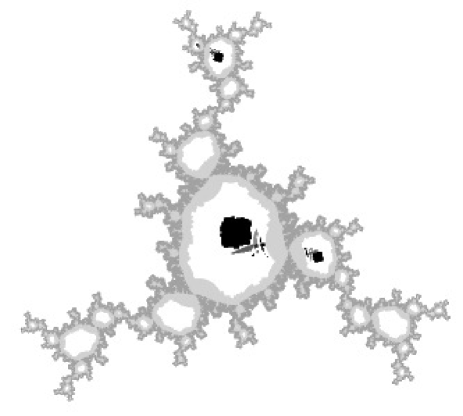
Figure 3. A box chain recurrent set for $P_{a,c}(z)=z^{3}-3a^{2}z+c,$ with $c=-.19+1.1i,a=0.1i$, and boxes from a $2^{10}\times 2^{10}$ grid on $[-2,2]^{2}$. Here $\mathcal{R}$ is $J$ and a 4-cycle. The black regions form the box chain transitive component of the 4-cycle. The origin lies in the center of the largest black region (in the center of the figure). The box chain transitive component containing $J$ is shaded two tones, to heuristically illustrate J. The distance from the origin to the end of any of the three limbs of $J$ is approximately $1.3$. The small shaded islands spread between $J$ and the 4-cycle neighborhood are several box chain transitive components which do not intersect $\mathcal{R}$, but are contained in some $\mathcal{R}({\varepsilon^{\prime}})$.

shows the box chain recurrent set which we computed using Hypatia. To get this approximation, we uniformly subdivided to obtain boxes from a $2^{10}\times 2^{10}$ grid on $[-2,2]^{2}$. Note there are several small box chain transitive components spread between $J$ and the 4-cycle, which cannot contain any points of $\mathcal{R}$, but by Corollary 2.17 these box chain transitive components are contained in some $\mathcal{R}({\varepsilon^{\prime}})$.

5.2. Drawing pictures of box chain recurrent sets for Hénon mappings

Since applying the box chain construction is an iterative process, we need feedback after each step $(n)$ to help us determine when to halt. In this paper, we consider a sucessful construction to be one which arrives at a fully separating box chain recurrent model (recall Definition 1.4).

To check heuristically whether a box chain recurrent model $\Gamma$ is separating, we take advantage of the fact that the unstable manifold, $W^{u}(p)$, of a saddle fixed point, $p$, can be (approximately) explicitly parameterized by the plane (details are given in Section A.3), and we sketch the slice of $\mathcal{B}$ lying in some $W^{u}(p)$.

This parameterization identifies $p$ with the origin, and conjugates the Hénon map to multiplication by the unstable eigenvalue. Hence a parameterized picture of $J\cap W^{u}(p)$ is invariant up to scaling by this eigenvalue, so the restriction to any neighborhood of $p$, $\mathcal{N}({p},{r})$, shows a fundamental domain. A box chain recurrent set $\mathcal{B}$ contains boxes of a certain size, so a parameterized $\mathcal{B}\cap W^{u}(p)$ is not quite invariant under scaling, but for many choices of $r$, a sketch of $\mathcal{B}\cap W^{u}(p)\cap\mathcal{N}({p},{r})$ will show us whether the box chain transitive components have separated $J$ from the sinks, and give an idea of how well $\mathcal{B}$ is approximating $J$, especially compared to a picture generated the same way with larger boxes (on a previous step).

To determine the coloration of a pixel, we check whether the pixel intersects some boxes in $\mathcal{B}$. The simplest picture would entail coloring a pixel black if it hits $\mathcal{B}$, or white if not. Going one step further, we illustrate the multiple box chain transitive components of $\Gamma$ by using multiple shades of grey. However, since our picture is a parametrization of a one complex dimensional manifold which does not line up with the axes in $\mathbb{C}^{{2}}$, a pixel may hit more than one box, and in more than one box chain transitive component. So, we use a color palette which has different shades of grey for each box chain transitive component, and a distinctive shade (like black) if the pixel hits more than one box chain transitive component.

We can also enhance our sketch in order to see how well a given box chain recurrent set approximates $\mathcal{R}$. Theorem A.1 (Section A.2) states that $J\subset\mathcal{R}\subset K$, and if $W^{u}(p)$ is the unstable manifold of any saddle periodic point, $p$, then clearly $W^{u}(p)\subset K^{-}$. Hence we slightly lighten the pixels which seem to be in $K^{+}$; i.e., the center point of the pixel stays small after several iterates of the map. In this way we can check visually how well $\mathcal{B}$ approximates $J$.

Note that since $W^{u}(p)\subset K^{-}$, the attracting periodic orbits of the map do not lie in $W^{u}(p)$. However, their basins of attraction can intersect $W^{u}(p)$. Thus in sketching box chain recurrent sets in this manner, we usually see part of the box chain transitive components corresponding to the sink orbits.

5.3. Complex Hénon mappings

Recall from Section 1 that if $f_{a,c}$ is a Hénon mapping with $a$ sufficiently small and $c$ is such that the polynomial $P_{c}(z)=z^{2}+c$ is hyperbolic (thus stable under perturbation), then $f|_{J}$ is topologically conjugate to the function induced by $P$ on the inverse limit ${\lim_{\leftarrow}(J,P)}$ ([14]). In this case, we say that $f$ is described by $P$, or simply that $f$ exhibits one dimensional behavior.

Example 5.2 (The alternate basilica).

Recall from Example 1.3 that the Hénon mapping $f_{a,c}$ with $c=-1.1875,a=.15$, seems to be one of the simplest Hénon mappings which does not exhibit one dimensional behavior. Computer evidence suggests that $\mathcal{R}$ consists of $J$ and an attracting two-cycle. We found the most efficient box chain construction for separating the sink from $J$ was to subdivide $\mathcal{B}_{0}$ initially with a $(2^{6})^{4}$ grid, then perform sink basin subdivision. In this way we acheived the left side of Figure 1 (shown in Section 1). To improve the approximation, we performed sink basin subdivision once more, and obtained the right side of Figure 1 (shown in Section 1). In these figures, note the box chain transitive components skirting the inner edge of the more refined $\mathcal{B}^{\prime}$. These would not be present for smaller box size, i.e., these components do not contain any points of $\mathcal{R}$, though they are contained in some $\mathcal{R}({\varepsilon^{\prime}})$.

Next we examine a different type of diffeomorphism: a horseshoe.

Definition 5.3.

A horseshoe is a diffeomorphism $f$ such that $f|_{J}$ is topologically conjugate to the left shift operator on $\Sigma_{2}$ (the symbol space of bi-infinite sequences of 0’s and 1’s). The horseshoe locus in the Hénon parameter space, $\mathcal{H}$, is the hyperbolic component of parameter space containing the set of horseshoes.

Since the full left shift on $\Sigma_{2}$ is the inverse limit of the one-sided left shift, horseshoes exhibit one dimensional behavior. All horseshoes are topologically the same as Smale’s horseshoe, i.e., the Julia set is a Cantor set, and the dynamics are well-understood.

However, pictures of the Hénon parameter space produced by SaddleDrop ([13]) suggest that the topology of the horseshoe locus is quite complicated. There are intriguing conjections about the horseshoe locus, which motivate the study of complex Hénon horseshoes. Below we describe one example of applying the box chain construction to a horseshoe.

Example 5.4.

The Hénon mapping with $c=-2.75,a=-.74$ appears to be a complex horseshoe—though parameters $c,a$ are real, the horseshoe for the map of $\mathbb{C}^{{2}}$ is not contained in $\mathbb{R}^{{2}}$. For horseshoe diffeomorphisms, there is no sink. Thus there is no clear option for selective subdivision. We simply had Hypatia uniformly subdivide the boxes, to obtain a box chain recurrent model consisting of boxes from a $(2^{6})^{2}$ grid on $\mathcal{B}_{0}=\mathcal{N}({0},{2.84})$. Since $J$ is a Cantor set, it is easiest to visualize $J$ via the FractalAsm picture shown on the left side of Figure 4.

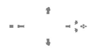
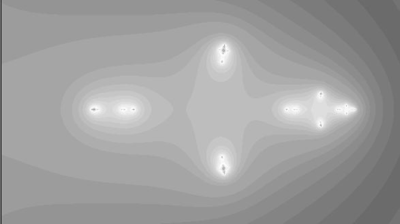
Figure 4. In these pictures, $f_{a,c}$ is the Hénon mapping with $a=-.74,c=-2.75$. This map appears to be a horseshoe, thus $\mathcal{R}=J$ appears to be a Cantor set. On the right is a parametrization of $W^{u}(p)$, where black is $W^{u}(p)\cap K^{+}$. On the left is a box chain recurrent set with boxes of size $2R^{\prime}/2^{6}$, for $R^{\prime}=2.84$.

The box chain recurrent set is shown on the right side of Figure 4. Actually, this cantor set was sparse enough that we were able to refine uniformly to a $(2^{10})^{2}$ grid, but at this point the picture was nearly impossible to see, since the set is very small.

5.4. Real Hénon mappings

The Hénon mapping is widely studied as a diffeomorphism of $\mathbb{R}^{{2}}$, with $a,c$ real parameters. In fact, for some complex Hénon mappings with real parameters, $\mathcal{R}$ lies in $\mathbb{R}^{{2}}$, and the complex dynamics can be completely described by studying the restriction to $\mathbb{R}^{{2}}$ (see [2]). Observe that all of the results of this paper apply immediately to the real setting. We implemented the box chain construction for real Hénon mappings in Hypatia; below is one example of a box chain recurrent set for a real Hénon mapping.

Example 5.5.

The Hénon mapping $f_{a,c}$ with $(a,c)=(-.25,-3)$ appears to be a real horseshoe, in that $\mathcal{R}=J$ seems to lie in $\mathbb{R}^{{2}}$. Thus a parameterized unstable manifold picture of the Julia set would simply show a Cantor set lying in the real axis. With Hypatia we constructed a box chain recurrent set using boxes from a $(2^{7}\times 2^{7})$ grid on $\mathcal{N}({0},{2.56})\subset\mathbb{R}^{{2}}.$ This box chain recurrent set (shown in $\mathbb{R}^{{2}}$) is on the left in Figure 5.

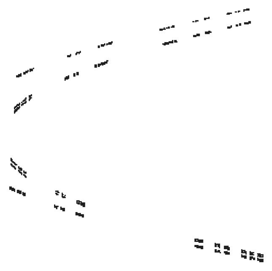
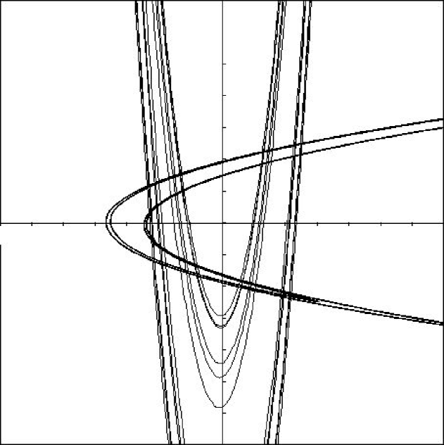
Figure 5. The Hénon mapping $f_{a,c}$ with $(a,c)=(-.25,-3)$ appears to be a real horseshoe, thus $\mathcal{R}=J\subset\mathbb{R}^{{2}}$ is a Cantor set. On the right is a sketch of the stable and unstable manifolds of a saddle fixed point, $W^{s}(p)\cup W^{u}(p)$, shown in the region $[-7,7]^{2}$. On the left is a box chain recurrent set $\mathcal{B}$ with boxes of size $2R^{\prime}/2^{7}$, where $R^{\prime}=2.56$. In fact, $\mathcal{B}$ is a neighborhood of the intersection $W^{s}(p)\cap W^{u}(p)$.

The reader familiar with the study of real Hénon mappings may recognize that the box chain recurrent set (on the left of Figure 5) appears to show an approximation to the intersection of the stable and unstable manifolds, $W^{u}(p)$ and $W^{s}(p)$ for some saddle periodic point $p$. Indeed, the right side of Figure 5 shows a sketch of such manifolds. This observation holds because for any Hénon mapping, $\overline{W^{u}(p)}\subset J^{-}$ and $\overline{W^{s}(p)}\subset J^{+}$ (see Section A). Thus $J=J^{+}\cap J^{-}=\overline{W^{s}(p)}\cap\overline{W^{u}(p)}$.

Table 2. Data for the box chain models constructed in the Examples of Section 5. Here $\Gamma^{\prime}$ denotes the box chain transitive component of $\Gamma$ which contains $J$, and the box grid depth for a box is the number $n$ such that the box is of size $2R^{\prime}/2^{n}$. If a box chain model contains boxes of multiple sizes, then multiple box grid depths are listed. Recall Example 5.1 is of a cubic polynomial $P_{a,c}(z)=z^{3}-3a^{2}z+c$, and the other examples are of Hénon mappings $f_{a,c}(x,y)=(x^{2}+c-ay,x)$.

Example		5.1	5.2		5.4	5.5
Figure		3	1	1	4	5
params.	$c$	$-.19+1.1i$	$-1.1875$		$-2.75$	$-3$
	$a$	$0.1i$	$0.15$		$-.74$	$-.25$
sink period		$4$	$2$		N/A	N/A
$\varepsilon^{\prime}$ s.t.	$\mathcal{B}\subset\mathcal{R}({\varepsilon^{\prime}+s(F)})$	$.028$	$0.30$	$0.30$	$0.68$	$0.26$
$\delta^{\prime}$s.t.	$\mathcal{R}({{\delta}^{\prime}})\subset\mathcal{B}$	$1.5\times 10^{-6}$	$6\times 10^{-6}$	$3\times 10^{-6}$	$1.2\times 10^{-5}$	$6.3\times 10^{-6}$
$R^{\prime}$		$2.1$	$1.9$		$2.84$	$2.57$
box grid depth, $n$		$11$	$6,7$	$6,7,8$	$6$	$7$
box size		$0.002$	$.06,.03$	$.06,.03,.015$	$0.09$	$0.04$
# $\Upsilon$ boxes	original	$98$	$184$	$682$	$60$	$20$
($1000$s)	$\mathcal{B}$-escaping	$0$	$116$	$417$	$43$	$15$
$\Upsilon$ size	boxes	$98$	$68$	$265$	$17$	$4$
($1000$s)	edges	$1{,}300$	$2{,}500$	$12{,}400$	$830$	$120$
$\Gamma^{\prime}$ size	boxes	$60$	$53$	$182$	$10$	$2.4$
($1000$s)	edges	$780$	$2{,}500$	$7{,}800$	$500$	$75$
runtime (min.)		$<5$		$20$	$<1$	$<1$
RAM (MB)		$<200$		$900$	$20$	$20$

Appendix A Background on Hénon mappings

A.1. The Hénon Family

Polynomial diffeomorphisms of $\mathbb{C}^{{2}}$ necessarily have polynomial inverses, thus are often called polynomial automorphisms. Friedland and Milnor ([9]) showed that polynomial automorphisms of $\mathbb{C}^{{2}}$ break down into two categories. Elementary automorphisms have simple dynamics, and are polynomially conjugate to a diffeomorphism of the form $(x,y)\mapsto(ax+b,cy+p(x))$ ($p$ polynomial, $a,c\neq 0$). Nonelementary automorphisms are all conjugate to finite compositions of generalized Hénon mappings, which are of the form $f(x,y)=(p(x)-ay,x)$, where $p(x)$ is a monic polynomial of degree $d>1$ and $a\neq 0$.

To clarify the situation, one can define a dynamical degree of a polynomial automorphism of $\mathbb{C}^{{2}}$. If deg$(f)$ is the maximum of the degrees of the coordinate functions, the dynamical degree is

$$d=d(f)=\lim_{n\to\infty}(\textit{deg}(f^{n}))^{1/n}.$$

This degree is a conjugacy invariant. Elementary automorphisms have dynamical degree $d=1$. A nonelementary automorphism is conjugate to some automorphism whose polynomial degree is equal to its dynamical degree. Without loss of generality, we assume such $f$ are finite compositions of generalized Hénon mappings, rather than merely conjugate to mappings of this form.

Thus, the quadratic, complex Hénon family $f_{a,c}(x,y)=(x^{2}+c-ay,x)$ represents the dynamical behavior of the simplest class of nonelementary polynomial automorphisms; those of dynamical degree two. We shall state results assuming $f$ is a polynomial diffeomorphism of $\mathbb{C}^{{2}}$ with $d(f)>1$, and often concentrate on the illustrative example of $f_{a,c}(x,y)=(x^{2}+c-ay,x)$.

A.2. Invariant sets of interest

The chain recurrent set, $\mathcal{R}$, and the Julia set, $J$, are both attempts at locating the points with dynamically interesting behavior. $\mathcal{R}$ can also be decomposed into components which do not interact with one another.

First we recall the key concepts associated to chain recurrence. An $\varepsilon$-chain of length $n>1$ from $p$ to $q$ is a sequence of points $\{p=x_{1},\ldots,x_{n}=q\}$ such that $\left\lvert f(x_{k})-x_{k+1}\right\rvert<\epsilon$ for $1\leq i\leq n-1.$ A point $p$ belongs to the $\varepsilon$-chain recurrent set, $\mathcal{R}({\varepsilon})$, of a function $f$ if there is an $\varepsilon$-chain from $p$ to $p$. The chain recurrent set is $\mathcal{R}=\cap_{\varepsilon>0}\mathcal{R}({\varepsilon}).$ A point $q$ is in the forward chain limit set of a point $p$, $\mathcal{R}(p)$, if for all $\varepsilon>0$, for all $n\geq 1$, there is an $\varepsilon$-chain from $p$ to $q$ of length greater than $n$. Put an equivalence relation on $\mathcal{R}$ by: $p\sim q$ if $p\in\mathcal{R}(q)$ and $q\in\mathcal{R}(p)$. Equivalence classes are called chain transitive components. We can define $\mathcal{R}({\varepsilon})(p)$ and $\varepsilon$-chain transitive components analogously. For ease of notation, we will sometimes refer to $\mathcal{R}$ as $\mathcal{R}({\varepsilon})$ for $\varepsilon=0$, or $\mathcal{R}(0)$. Note that $\mathcal{R}$ is closed and invariant, and if $\varepsilon<\varepsilon^{\prime}$, then $\mathcal{R}\subset\mathcal{R}({\varepsilon})\subset\mathcal{R}({\varepsilon^{\prime}})$.

Chain recurrence is quite natural to rigorously study using a computer. A box chain recurrent model $\Gamma$ is an approximation to the dynamics of $f$ on $\mathcal{R}$, and the connected components of $\Gamma$ are approximations to the chain transitive components. This is made precise in Section 2.

For a polynomial map $f$ of $\mathbb{C}$, the filled Julia set, $K$, is the set of points whose orbits are bounded under $f$; the Julia set, $J$, is the topological boundary of $K$. For a polynomial diffeomorphism $f$ of $\mathbb{C}^{{2}}$, there are corresponding Julia sets: $K^{+}(K^{-})$ is the set of points whose orbits are bounded under $f(f^{-1})$ and $K=K^{+}\cap K^{-}$ is called the filled Julia set; $J^{\pm}=\partial K^{\pm}$ (the topological boundary) and $J=J^{+}\cap J^{-}$ is called the Julia set. The Julia set can be easily sketched by computer, and is also extensively used in formulating theoretical results for complex Hénon mappings.

Bedford and Smillie show the following relationships between $\mathcal{R}$ and $J$

Theorem A.1 ([3]).

Let $f$ be a polynomial diffeomorphism of $\mathbb{C}^{{2}}$, with $d(f)>1$.

1. Then $J\subset\mathcal{R}\subset K$ and $J$ is contained in a single chain transitive component of $\mathcal{R}$.

2. Assume further that $\left\lvert\text{det}Df\right\rvert<1$. Let $O_{j}$ for $j=1,2,\ldots$ denote the sink orbits of $f$.

   1. Then $\mathcal{R}$ is the set of bounded orbits (in forward/backward time) not in punctured basins, where if $p$ is a sink, the punctured basin of $p$ is $W^{s}(p)-p$, and

   2. the chain transitive components are the sink orbits, $O_{j}$, and the set $\mathcal{R}-\cup_{j}O_{j}$.

A.3. Drawing Meaningful pictures for maps of $\mathbb{C}^{{2}}$

Filled Julia sets are the invariant sets which can be easily sketched by computer, on any two-dimensional slice. Hubbard has suggested the following method for drawing a dynamically significant slice of the Julia set of a Hénon mapping, by parameterizing an unstable manifold. This method has been implemented by Karl Papadantonakis into a program called FractalAsm, available for download at [1]. We also use this method to draw pictures of collections of boxes, see Sections 1 and 5 for examples.

Let $f$ be a diffeomorphism of $\mathbb{C}^{{2}}$. If $p$ is a periodic point of period $m$, and the eigenvalues $\lambda,\mu$ of $D_{p}f^{m}$ satisfy $\left\lvert\lambda\right\rvert>1>\left\lvert\mu\right\rvert$ (or vice-versa), then $p$ is a saddle periodic point. The large (small) eigenvalue is called the unstable (stable) eigenvalue. If $p$ is a saddle periodic point, then the stable manifold of $p$ is $W^{s}(p)=\{q\colon d(f^{n}(q),f^{n}(p))\rightarrow 0\text{ as }n\rightarrow\infty\},$ and the unstable manifold of $p$ is $W^{u}(p)=\{q\colon d(f^{-n}(q),f^{-n}(p))\rightarrow 0\text{ as }n\rightarrow\infty\}.$ If $p$ a saddle periodic point of $f$, then $W^{u}(p)\ (W^{s}(p))$ is biholomorphically equivalent to $\mathbb{C}$, and on $W^{u}(p)\ (W^{s}(p))$, $f$ is conjugate to multiplication by the unstable (stable) eigenvalue of $D_{p}f$.

Let $f$ be a Hénon mapping. When $\left\lvert a\right\rvert\neq 1$, except on the curve of equation $4c=(1+a)^{2}$, the map $f_{a,c}$ has at least one saddle fixed point, $p$, ([13]). The unstable manifold $W^{u}(p)$ has a natural parametrization $\gamma\colon\mathbb{C}\to W^{u}(p)$ given by

$$\gamma(z)=\lim_{m\to\infty}\gamma_{m}(z)=\lim_{m\to\infty}f^{m}\left(p+\frac{z}{\lambda_{1}^{m}}\mathbf{v_{1}}\right),$$

where $\lambda_{1}$ is the unstable eigenvalue of $D_{p}f$ and $\mathbf{v_{1}}$ is the associated eigenvector. This parametrization has the property that $f(\gamma(z))=\gamma(\lambda z),$ and any two parametrizations with this property differ by scaling the argument.

To parameterize $W^{u}(p)$, we approximate $\gamma$ by some $g=\gamma_{N}$ in a region in the plane: $B=\{z=x+iy\colon a\leq x\leq b,c\leq y\leq d\}$. Observe that since $W^{u}(p)\subset K^{-}$, to sketch $K$ in $W^{u}(p)$, we need only sketch $K^{+}$. Thus for each pixel $Z\in B$, if $f^{n}(g(Z))$ is bounded by some $R$ for all $n<N$, we guess $g(Z)\in K^{+}$ and color $Z$ black. Otherwise, color according to which iterate $f^{n}(g(Z))$ first surpassed $R$.

Appendix B Rigorous Arithmetic

On a computer, we cannot work with real numbers; instead we work over the finite space $\mathbb{F}$ of numbers representable by binary floating point numbers no longer than a certain length. For example, since the number $0.1$ is not a dyadic rational, it has an infinite binary expansion. Thus the computer cannot encode $0.1$ exactly. Interval arithmetic (IA) provides a method for maintaining rigor in computations, and also is natural and efficient for manipulating boxes. The basic objects of IA are closed intervals, $[a]=[\underline{a},\bar{a}]\in\mathbb{I}\mathbb{K}$, with end points in some fixed field, $\mathbb{K}$. An arithmetical operation on two intervals produces a resulting interval which contains the real answer. For example,

$$[a]+[b] :=\left[\underline{a}+\underline{b},\bar{a}+\bar{b}\right]$$

$$[a]-[b] :=\left[\underline{a}-\bar{b},\bar{a}-\underline{b}\right]$$

Multiplication and division can also be defined in IA.

Since an arithmetical operation on two computer numbers in $\mathbb{F}$ may not have a result in $\mathbb{F}$, in order to implement rigorous IA we must round outward the result of any interval arithmetic operation, e.g. for $[a],[b]\in\mathbb{I}\mathbb{F}$,

$$[a]+[b]:=\left[\left\downarrow\underline{a}+\underline{b}\right\downarrow,\left\uparrow\bar{a}+\bar{b}\right\uparrow\right],$$

where $\left\downarrow x\right\downarrow$ denotes the largest number in $\mathbb{F}$ that is strictly less than $x$ (i.e., $x$ rounded down), and $\left\uparrow x\right\uparrow$ denotes the smallest number in $\mathbb{F}$ that is strictly greater than $x$ (i.e., $x$ rounded up). This is called IA with directed rounding.

For any $x\in\mathbb{R}$, let Hull$(x)$ be the smallest interval in $\mathbb{F}$ which contains $x$. That is, if $x\in\mathbb{F}$, then Hull$(x)$ denotes $[x,x]$. If $x\in\mathbb{R}\setminus\mathbb{F}$, then Hull$(x)$ denotes $\left[\left\downarrow x\right\downarrow,\left\uparrow x\right\uparrow\right]$. Similarly, for a set $S\subset\mathbb{R}$, we say Hull$(S)$ for the smallest interval containg $S$. Whether Hull$(S)$ is in $\mathbb{I}\mathbb{R}$ or $\mathbb{I}\mathbb{F}$ should be clear from context.

In higher dimensions, IA operations can be carried out component-wise, on interval vectors. So if $x\in\mathbb{R}^{{n}}$, then Hull$(x)=\text{ Hull}(x_{1})\times\cdots\times\text{ Hull}(x_{n})$, and if $S\subset\mathbb{R}^{{n}}$, then $\text{Hull}(S)$ is the smallest vector in $\mathbb{I}\mathbb{F}^{n}$ (or $\mathbb{I}\mathbb{R}^{n}$) containing $S$. Note to deal with intervals in $\mathbb{C}^{{n}}$ we simply identify $\mathbb{C}^{{n}}$ with $\mathbb{R}^{2n}$. Thus a box in $\mathbb{C}=\mathbb{R}^{{2}}$ is an interval vector of length two. Our extensive use of boxes is designed to make IA calculations natural.

To compute the image of a point $x$ under a map $f$ using IA, first convert $x$ to an interval vector $X=\text{ Hull}(x)$, then use a (carefully chosen) combination of the basic arithmetical operations to compute an interval vector $F(X)$, such that we are guaranteed that Hull$(f(x))\subset F(X)$.

Definition B.1.

Let $f\colon\mathbb{R}^{{n}}\to\mathbb{R}^{{n}}$ be continuous. An interval extension of $f$, $F=F(f)$, is a function which maps a box $B$ in $\mathbb{R}^{{n}}$ to a box $F(B)$ containing $f(B)$, i.e., $F(B)\supset\text{Hull}(f(B))$.

Usually, we would like $F(B)$ to be as close as possible to Hull($f(B)$). We shall not discuss how to find the best $F$. However, in this paper we do distinguish between $F(B)$ and Hull$(f(B))$ when stating our results, to make clear the difference between theory and practice.

Each time an arithmetical calculation is performed, one must think carefully about how to use IA. For example, IA is not distributive. Also, it can easily create large error propagation. For example, iterating a polynomial map or diffeomorphism on an interval vector (which is not very close to an attracting period cycle) will usually produce a very large interval vector after only a few iterates. That is, if $B$ is a box in $\mathbb{R}^{{2}}=\mathbb{C}$, and one attempts to compute a box containing $f_{c}^{10}(B)$, for $f_{c}(z)=z^{2}+c$, by:

for $j$ from $1$ to $10$ do
	$B=F_{c}(B)$

then the box $B$ will likely grow so large that its defining bounds become machine $\infty$, i.e., the largest floating point in $\mathbb{F}$. Similarly, if $f$ is a Hénon mapping, one would also never want to try to compute $D_{B_{n}}f\circ\cdots\circ D_{B_{1}}f\circ D_{B_{0}}f(\mathbf{u}),$ for a vector $\mathbf{u}\in\mathbb{C}^{{2}}$, since the entries would blow up.

We use IA for all the rigorous computations in the computer program Hypatia. The IA routines were all provided by the PROFIL/BIAS package, available at [22]. For further background on interval arithmetic, see [4, 16, 17].

References

- [1] Dynamics at Cornell. [http://www.math.cornell.edu/~dynamics].
- [2] E. Bedford and J. Smillie. Polynomial diffeomorphisms of : currents, equilibrium measure and hyperbolicity. Invent. Math., 103(1):69–99, 1991.
- [3] E. Bedford and J. Smillie. Polynomial diffeomorphisms of . II. Stable manifolds and recurrence. J. Amer. Math. Soc., 4(4):657–679, 1991.
- [4] Interval Computations. [http://www.cs.utep.edu/interval-comp/].
- [5] T. Cormen et al. Introduction to Algorithms. The MIT Electrical Engineering and Computer Science Series. The MIT Press and McGraw-Hill Book Company, 1990.
- [6] M. Dellnitz and A. Hohmann. A subdivision algorithm for the computation of unstable manifolds and global attractors. Numer. Math., 75(3):293–317, 1997.
- [7] M. Dellnitz and O. Junge. Set oriented numerical methods for dynamical systems. In Handbook of dynamical systems, Vol. 2, pages 221–264. North-Holland, Amsterdam, 2002.
- [8] M. Eidenschink. Exploring Global Dynamics: A Numerical Algorithm Based on the Conley Index Theory. PhD thesis, Georgia Institute of Technology, 1995.
- [9] S. Friedland and J. Milnor. Dynamical properties of plane polynomial automorphisms. Ergodic Theory Dynamical Systems, 9(1):67–99, 1989.
- [10] J.S.L. Hruska. On the numerical construction of hyperbolic structures for complex dynamical systems. PhD thesis, Cornell University, 2002. Available for download at the Stony Brook Dynamical Systems Thesis Server [http://www.math.sunysb.edu/dynamics/theses/index.html].
- [11] S. L. Hruska. A numerical method for proving hyperbolicity of complex Hénon mappings. submitted, preprint available at [http://xxx.arxiv.org].
- [12] S.L. Hruska. Constructing an expanding metric for dynamical systems in one complex variable. 2005.
- [13] J. Hubbard and K. Papadantonakis. Exploring the parameter space of complex Hénon mappings. Journal of Experimental Mathematics, to appear.
- [14] J.H. Hubbard and R.W. Oberste-Vorth. Hénon mappings in the complex domain. II. projective and inductive limits of polynomials. In B. Branner and P. Hjorth, editors, Real and Complex Dynamical Systems, volume 464 of NATO Adv. Sci. Inst. Ser. C Math. Phys. Sci., pages 89–132. Kluwer Acad. Publ., Dordrecht, 1995.
- [15] K. Mischaikow. Topological techniques for efficient rigorous computations in dynamics. Acta Numerica, 11:435–477, 2002.
- [16] R.E. Moore. Interval Analysis. Prentice-Hall, Englewood Cliffs, New Jersey, 1966.
- [17] R.E. Moore. Methods and Applications of Interval Analysis. SIAM Studies in Applied Mathematics, Philadelphia, 1979.
- [18] R. Oliva. On the combinatorics of external rays in the dynamics of the complex Hénon map. PhD thesis, Cornell University, 1998.
- [19] G. Osipenko. On the symbolic image of a dynamical system. In Boundary value problems (Russian), pages 101–105, 198. Perm. Politekh. Inst., Perm′, 1983.
- [20] G. Osipenko. Construction of attractors and filtrations. In Conley index theory (Warsaw, 1997), volume 47 of Banach Center Publ., pages 173–192. Polish Acad. Sci., Warsaw, 1999.
- [21] G. Osipenko and S. Campbell. Applied symbolic dynamics: attractors and filtrations. Discrete Contin. Dynam. Systems, 5(1):43–60, 1999.
- [22] PROFIL/BIAS Interval Arithmetic Package. [http://www.ti3.tu-harburg.de/Software/PROFILEnglisch.html].
- [23] J. Smillie. The entropy of polynomial diffeomorphisms of . Ergodic Theory Dynam. Systems, 10(4):823–827, 1990.
- [24] W. Tucker. A rigorous ODE solver and Smale’s 14th problem. Found. Comput. Math., 2(1):53–117, 2002.