Neighborhood complexes and generating functions for affine semigroups

Abstract

Given $a_{1},a_{2},\ldots,a_{n}\in\mathbb{Z}^{d}$, we examine the set, G, of all non-negative integer combinations of these $a_{i}$. In particular, we examine the generating function $f(\mathbf{z})=\sum_{b\in G}\mathbf{z}^{b}$. We prove that one can write this generating function as a rational function using the neighborhood complex (sometimes called the complex of maximal lattice-free bodies or the Scarf complex) on a particular lattice in $\mathbb{Z}^{n}$. In the generic case, this follows from algebraic results of D. Bayer and B. Sturmfels. Here we prove it geometrically in all cases, and we examine a generalization involving the neighborhood complex on an arbitrary lattice.

1 Introduction

Given positive integers $a_{1},a_{2},\ldots,a_{n}$, let

$$G=\{\mu_{1}a_{1}+\mu_{2}a_{2}+\cdots+\mu_{n}a_{n}:\ \mu_{i}\in\mathbb{Z}_{\geq 0}\}.$$

In other words, $G$ is the additive semigroup (with zero) generated by $a_{1},a_{2},\ldots,a_{n}$. If the greatest common divisor of $a_{1},a_{2},\ldots,a_{n}$ is one, then all sufficiently large integers are in $G$, and the Frobenius problem is to find the largest integer not in $G$. We would like to say something about the structure of the set $G$. In particular, define the generating function

$$f(z)=\sum_{b\in G}z^{b}.$$

This generating function converges for $\lvert z\rvert<1$. We would like to calculate $f(z)$ in a nice form. It will turn out that we can obtain it from the neighborhood complex (sometimes called the Scarf complex or the complex of maximal lattice-free bodies; we will define it shortly) of an associated lattice. This was proved by D. Bayer and B. Sturmfels using algebraic methods [6]. Here we prove it geometrically.

We do not need to restrict ourselves to the case where $G$ is one dimensional. In general, Let $A$ be a $d\times n$ matrix of integers with columns $a_{1},a_{2},\ldots,a_{n}\in\mathbb{Z}^{d}$, and define

$$G=\{\mu_{1}a_{1}+\mu_{2}a_{2}+\cdots+\mu_{n}a_{n}:\ \mu_{i}\in\mathbb{Z}_{\geq 0}\}=\{A\xi:\ \xi\in\mathbb{Z}^{n}_{\geq 0}\}.$$

Then the $d=1$ case corresponds to the Frobenius problem. Define the generating function

$$f(\mathbf{z})=\sum_{b\in G}\mathbf{z}^{b}=\sum_{b=(b_{1},\ldots,b_{d})\in G}z_{1}^{b_{1}}z_{2}^{b_{2}}\cdots z_{d}^{b_{d}},$$

where $\mathbf{z}=(z_{1},z_{2},\ldots,z_{d})$. We assume that there exists an $l=(l_{1},l_{2},\ldots,l_{d})\in\mathbb{R}^{d}$ such that $\langle l,a_{i}\rangle<0$ for all $i$. Then for all $\mathbf{z}$ in a neighborhood of $(e^{l_{1}},e^{l_{2}},\ldots,e^{l_{d}})$ we have $\lVert\mathbf{z}^{a_{i}}\rVert<1$, and so $f(\mathbf{z})$ will converge in this neighborhood. Note that if there were no such $l$, then $G$ would contain a linear subgroup, and $f(\mathbf{z})$ would not converge on any open subset of $\mathbb{C}^{d}$. Since the structure of a linear group is simple, however, we are not concerned with such $G$.

We would like to calculate this generating function, $f(\mathbf{z})$. Theorem 1.3 gives the answer.

Let $\Lambda\subset\mathbb{Z}^{n}$ be the lattice

$$\{\lambda\in\mathbb{Z}^{n}:\ A\lambda=0\}.$$

We will shortly define the neighborhood complex, $S$, a simplicial complex whose vertices are $\Lambda$. By a simplicial complex, we mean that $S$ is a collection of finite subsets of $\Lambda$, and that if $s\in S$, then all subsets of $s$ are also in $S$. The vertices of the complex are the $\{s\}\in S$, the edges are the $\{s,s^{\prime}\}\in S$, and so forth. In this paper, we will not count the empty set as a simplex of $S$. This complex will not, in general, be geometrically realizable in the linear span of $\Lambda$.

For $s=\{\lambda^{1},\lambda^{2},\ldots,\lambda^{k}\}$ with $\lambda^{i}\in\Lambda$, define

$$\max(s)=\max\{\lambda^{1},\lambda^{2},\ldots,\lambda^{k}\},$$

where the maximum is taken coordinate-wise (for example, $\max\left\{(1,-1),(0,0)\right\}=(1,0)$). We say that $\Lambda$ is generic if, whenever some nonzero $\lambda=(\lambda_{1},\lambda_{2},\ldots,\lambda_{n})\in\Lambda$ has $\lambda_{i}=0$, for some $i$, then there is a $\lambda^{\prime}\in\Lambda$ with $\lambda^{\prime}<\max(\lambda,0)$.

When $\Lambda$ is generic, define $S$, as follows. We have $s$ is in $S$ if and only if for no $\lambda\in\Lambda$ is $\lambda<\max(s)$. If $s\in S$, then all subsets of $s$ are in $S$ as well, so $S$ is a simplicial complex. In Section 5, we will define $S$ in the non-generic case. Basically, we must perturb the vertices slightly so we are in the generic case.

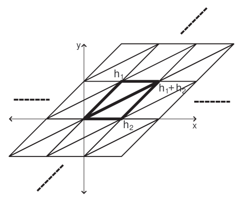
Figure 1.1: Example 1.2, the neighborhood complex (transformed to lie on $\mathbb{Z}^{2}$) when $A$ is a $1\times 3$ matrix.

Example 1.2.

If $A$ is a $1\times 3$ matrix (that is, $G$ is a one-dimensional additive semigroup with three generators), then $\Lambda$ is a two-dimensional sublattice of $\mathbb{Z}^{3}$. There exists a basis $\{h^{1},h^{2}\}$ of $\Lambda$ such that the neighborhood complex consists of vertices $\{x\}$, for $x\in\Lambda$; edges $\{x,x+h^{1}\},$ $\{x,x+h^{2}\}$, and $\{x,x+h^{1}+h^{2}\}$; and triangles $\{x,x+h^{1},x+h^{1}+h^{2}\}$ and $\{x,x+h^{2},x+h^{1}+h^{2}\}$ (see Figure 1.1, where $\Lambda$ has been transformed to be $\mathbb{Z}^{2}$, and see, for example, [13]). Notice that these triangles exactly tile the linear span of $\Lambda$. This is not true in higher dimensions.

Neighborhood complexes often appear in integer programming in a slightly different, but equivalent, form. Let $r$ be the dimension of the lattice $\Lambda$, and let $B$ be an $n\times r$ integer matrix whose columns form a basis for $\Lambda$, so that $\Lambda=\{Bx:\ x\in\mathbb{Z}^{r}\}$. Then we may form a simplicial complex, $S^{\prime}$, on $\mathbb{Z}^{r}$, as follows. Given $s^{\prime}=\{x^{1},x^{2},\ldots,x^{k}\}\subset\mathbb{Z}^{r}$, let $P_{s^{\prime}}$ be the polytope defined by

$$P_{s^{\prime}}=\big{\{}x\in\mathbb{R}^{r}:\ Bx\leq\max\{Bx^{1},Bx^{2},\ldots,Bx^{k}\}\big{\}}.$$

$P_{s^{\prime}}$ is the smallest polytope of any $\{x:\ Bx\leq b\}$, for $b\in\mathbb{Z}^{n}$, which contains $s^{\prime}$. In the generic case, we say that $s^{\prime}\in S^{\prime}$ if and only if $P_{s^{\prime}}$ contains no integer points in its interior. It is easily seen that $S^{\prime}$ and $S$ are isomorphic under the map $x\mapsto Bx$.

If $\{0,x^{\prime}\}\in S^{\prime}$ is an edge of the complex, then $x^{\prime}$ is called a neighbor of the origin. The set of neighbors of the origin form a test set for the family of integer programs

$$\text{minimize }\langle\beta_{n},x\rangle\text{ such that }\langle\beta_{i},x\rangle\leq b_{i},\text{ for }1\leq i\leq n-1,$$

where $\beta_{i}$ is the $i$th row of $B$ and $b=(b_{1},b_{2},\ldots,b_{n-1})$ is allowed to vary in $\mathbb{Z}^{n-1}$, and where $\langle\cdot,\cdot\rangle$ is the standard dot product on $\mathbb{R}^{r}$. The set of neighbors is a test set, because, for a fixed $b$, if $x$ is a feasible solution (that is, it satisfies the linear inequalities), then $x$ minimizes $\langle\beta_{n},x\rangle$ if and only if there is no neighbor, $x^{\prime}$, of the origin such that both $x-x^{\prime}$ is feasible and $\langle\beta_{n},x-x^{\prime}\rangle<\langle\beta_{n},x\rangle$. For an introduction to neighbors and their applications to integer programming, see [13].

Returning to $S$, the complex with vertices in $\Lambda$, we see that $S$ is invariant under translation by $\Lambda$. Let $\bar{S}$ be a set of distinct representatives of $S$ modulo $\Lambda$. Let

$$f_{\bar{S}}(\mathbf{z})=\frac{\sum_{s\in\bar{S}}(-1)^{\dim(s)}\mathbf{z}^{A\cdot\max(s)}}{\prod(1-\mathbf{z}^{a_{i}})}.$$

The following theorem states that this is the generating function that we are looking for.

Theorem 1.3.

Given a $d\times n$ matrix of integers $A$, let $\Lambda=\{\lambda\in\mathbb{Z}^{n}:\ A\lambda=0\}$. Define the neighborhood complex $S$ on $\Lambda$ as above (we define $S$ in the non-generic case in Section 5), and let $\bar{S}$ be a set of distinct representatives of $S$ modulo $\Lambda$. If $f(\mathbf{z})$ and $f_{\bar{S}}(\mathbf{z})$ are defined as above, then

$$f(\mathbf{z})=f_{\bar{S}}(\mathbf{z}).$$

In the generic case, this theorem follows from algebraic results of D. Bayer and B. Sturmfels [6], but we prove it here using elementary geometric methods. Bayer and Sturmfels construct the hull complex, which coincides with $\bar{S}$ when $\Lambda$ is generic, but which is larger than $\bar{S}$ in the non-generic case. Note that they use Hilbert series terminology, which is equivalent, because $f(\mathbf{z})$ is the Hilbert series for the monomial ring $\mathbb{C}[\mathbf{x}^{a_{1}},\mathbf{x}^{a_{2}},\ldots,\mathbf{x}^{a_{n}}]$ with the standard $\mathbb{Z}^{d}$-grading. A. Barvinok and K. Woods show [4] that $f(\mathbf{z})$ can be written as a “short” rational generating function (much shorter than $f_{\bar{S}}(\mathbf{z}))$, but, when written in that form, the structure of the neighborhood complex is lost.

The function $f_{\bar{S}}(\mathbf{z})$ makes sense even if $\Lambda$ is a proper sublattice (perhaps of full dimension, perhaps not) of $\{\lambda\in\mathbb{Z}^{n}:\ A\lambda=0\}$. That is, we may still define the neighborhood complex, $S$, and then take $\bar{S}$, a set of distinct representatives of $S$ modulo $\Lambda$, and define $f_{\bar{S}}(\mathbf{z})$ as above. Does $f_{\bar{S}}$ have an interpretation as a generating function, as in Theorem 1.3?

In fact, it does, as follows. Let $\Lambda$ be any lattice in $\mathbb{Z}^{n}$ such that $A\lambda=0$, for all $\lambda\in\Lambda$. Given $b\in\mathbb{Z}^{d}$, define

$$T_{b}=\{\xi\in\mathbb{Z}^{n}:\ \xi\geq 0\text{ and }A\xi=b\}.$$

That is, $T_{b}$ represents the set of ways to write $b$ as a nonnegative integer combination of the $a_{1},a_{2},\ldots,a_{n}$ (and so $T_{b}$ is nonempty if and only if $b$ is in the semigroup $G$). Define an equivalence relation on $T_{b}$ by

$$\xi\sim\eta\text{ iff }\xi-\eta\in\Lambda.$$

Let $c_{b}$ be the number of equivalence classes in $T_{b}$. Then we have the following theorem, which says that the $c_{b}$ are the coefficients of the Laurent power series $f_{\bar{S}}(\mathbf{z})$.

Theorem 1.4.

Given a $d\times n$ matrix of integers $A$ and a lattice $\Lambda\in\mathbb{Z}^{n}$ such that $A\lambda=0$ for all $\lambda\in\Lambda$, define the neighborhood complex $S$ on $\Lambda$ as above, and let $\bar{S}$ be a set of distinct representatives of $S$ modulo $\Lambda$. If $f_{\bar{S}}(\mathbf{z})$ and $c_{b}$ are defined as above, then

$$f_{\bar{S}}(\mathbf{z})=\sum_{b\in\mathbb{Z}^{d}}c_{b}\mathbf{z}^{b}.$$

When $\Lambda$ is a generic lattice, this theorem can be retrieved from a result of I. Peeva and B. Sturmfels [11], but they again use algebraic methods. In the case where $\Lambda$ is the full lattice $\{\lambda\in\mathbb{Z}^{n}:\ A\lambda=0\}$, every element of $T_{b}$ is equivalent to every other, since if $A\xi=A\eta=b$, then $A\cdot(\xi-\eta)=0$ and so $\xi-\eta\in\Lambda$. In this case, if $b\in G$ then $c_{b}=1$ (and if $b\notin G$ then $c_{b}=0$), and we recover Theorem 1.3.

At the other extreme, if $\Lambda=\{0\}$, each element of $T_{b}$ is in its own equivalence class. Then, since $S$ is the complex with one vertex $0$, we have

$$f_{\bar{S}}(\mathbf{z})=\frac{1}{\prod(1-\mathbf{z}^{a_{i}})},$$

and Theorem 1.4, in this case, is clear. We will present other examples of Theorems 1.3 and 1.4 in Section 2.

Let $L$ be the full orthogonal lattice $\{\ell\in\mathbb{Z}^{n}:\ A\ell=0\}$, and let $C$ be a lattice invariant simplicial complex on $L$. Note that when the lattice $\Lambda$ in Theorem 1.4 is not all of $L$, then $S$ itself is not $L$-invariant. In this case, if $\bar{L}$ is a set of distinct representatives of $L$ modulo $\Lambda$, then the complex $C$ we will examine will be the disjoint union

$$C=\bigcup_{\ell\in\bar{L}}S+\ell,$$

where

$$S+\ell=\big{\{}\{\lambda^{1}+\ell,\lambda^{2}+\ell,\ldots,\lambda^{k}+\ell\}:\ \{\lambda^{1},\lambda^{2},\ldots,\lambda^{k}\}\in S\big{\}},$$

which is $L$-invariant.

Define $C_{\xi}$ to be the subcomplex of $C$ consisting of simplices $s\in C$ such that

$$\max(s)\leq\xi.$$

$C_{\xi}$ is a simplicial complex, though it need not be pure (that is, its maximal simplices may not all be of the same dimension).

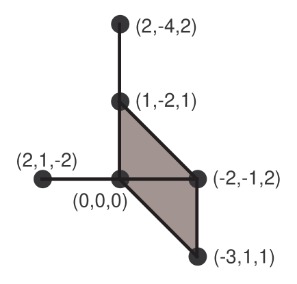
Figure 1.5: $C_{\xi}$ from Example 1.6

Example 1.6.

Let $A=[3\ 4\ 5]$ so that $G$ is the additive semigroup generated by 3, 4, and 5. Let $\Lambda=L=\{\lambda\in\mathbb{Z}^{3}:\ A\lambda=0\}$, and let $C=S$ be the neighborhood complex defined on $\Lambda$. One can show that $C$ has vertices $\{\lambda\}$, for $\lambda\in\Lambda$; edges $\{\lambda,\lambda+(2,1,-2)\},$ $\{\lambda,\lambda+(1,-2,1)\}$, and $\{\lambda,\lambda+(3,-1,-1)\}$; and triangles $\{\lambda,\lambda+(2,1,-2),\lambda+(3,-1,-1)\}$ and $\{\lambda,\lambda+(1,-2,1),\lambda+(3,-1,-1)\}$.

Let $\xi=(2,1,2)$. Then Figure 1.5 shows $C_{\xi}$. Note that, if $\{\lambda\}$ is a vertex of $C_{\xi}$, then $\xi-\lambda\geq 0$ by definition of $C_{\xi}$, and

$$A(\xi-\lambda)=A\xi=20,$$

and so (as will be important later), each vertex of $C_{\xi}$ corresponds to a way to write 20 as a nonnegative integer combination of 3,4, and 5. For example, $\{(1,-2,1)\}$ is a vertex of $C_{\xi}$, $\xi-(1,-2,1)=(1,3,1)$, and $1\cdot 3+3\cdot 4+1\cdot 5=20$.

Define the Euler characteristic, EC$(C_{\xi})$, by

$$\text{EC}(C_{\xi})=\sum_{s\in C_{\xi}}(-1)^{\dim(s)}.$$

Since $C$ is $L$-invariant, $C_{\xi-\ell}=C_{\xi}-\ell$ for all $\ell\in L$. Then, given $b\in\mathbb{Z}^{d}$, all of the $C_{\xi}$, for $\xi\in\mathbb{Z}^{n}$ such that $A\xi=b$, are isomorphic to each other, and we can define

$$d_{b}=\text{EC}(C_{\xi}),\text{ for some (any) }\xi\text{ such that }A\xi=b.$$

We will prove Theorems 1.3 and 1.4 using the following lemma, which says that these Euler characteristics, $d_{b}$, are the coefficients of the Laurent power series $f_{\bar{C}}(\mathbf{z})$.

Lemma 1.7.

If $A$ is a $d\times n$ matrix of integers and $C$ is a lattice invariant simplicial complex on $L=\{\ell\in\mathbb{Z}^{n}:\ A\ell=0\}$, let $d_{b}$ be defined as above, for all $b\in\mathbb{Z}^{d}$. If $\bar{C}$ is a set of distinct representatives of $C$ modulo $L$, then

$$f_{\bar{C}}(\mathbf{z})=\sum_{b\in\mathbb{Z}^{d}}d_{b}\mathbf{z}^{b},$$

where

$$f_{\bar{C}}(\mathbf{z})=\frac{\sum_{s\in\bar{C}}(-1)^{\dim(s)}\mathbf{z}^{A\cdot\max(s)}}{\prod(1-\mathbf{z}^{a_{i}})}.$$

We will prove this lemma in Section 3. First, in Section 2, we will give several examples of Theorems 1.3 and 1.4. In Section 4, we examine neighborhood complexes and make the Euler characteristic calculations necessary to prove Theorems 1.3 and 1.4 from Lemma 1.7. The key ingredient in these calculations will be the fact (first proved in [1]) that these neighborhood complexes have a very nice topological structure. In Section 5, we examine the non-generic case, and prove Theorems 1.3 and 1.4 for these lattices.

2 Examples

In this section, we look at several examples of Theorems 1.3 and 1.4. First we examine Theorem 1.3, for varying $n$ and $d$.

Suppose $d=1$. If $a_{1},a_{2},\ldots,a_{n}$ are positive integers whose greatest common divisor is one, then the Frobenius number is the largest integer not in $G$. The problem of finding this number dates back to Frobenius and Sylvester. H. Scarf and D. Shallcross [14] have related the Frobenius number itself to the neighborhood complex. They show (using slightly different terminology) that, if

$$N=\max\{A\cdot\max(s):\ s\text{ is in the neighborhood complex, }S\},$$

then the Frobenius number is

$$N-(a_{1}+a_{2}+\cdots+a_{n}).$$

Note that, in the terminology of this paper, $N$ is the largest exponent in the numerator of $f_{\bar{S}}(\mathbf{z})=f(\mathbf{z})$.

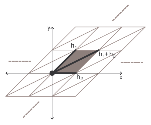
Figure 2.1: $\bar{C}$ (transformed to have vertices $\mathbb{Z}^{2}$), for $d=1,n=3$ in Example 2.3

Example 2.2.

Theorem 1.3, with $d=1,n=2$. Then

$$f(z)=\frac{1-z^{\text{lcm}(a_{1},a_{2})}}{(1-z^{a_{1}})(1-z^{a_{2}})}.$$

In this case, we may choose $\bar{S}$ to consist of the vertex $\{0\}$ and the edge $\{0,h\}$, where $h$ is a generator of the lattice $\Lambda$. This formula can easily be verified directly.

Example 2.3.

Theorem 1.3, with $d=1,n=3$. Then

$$f(z)=\frac{poly(z)}{(1-z^{a_{1}})(1-z^{a_{2}})(1-z^{a_{3}})},$$

where $poly(z)$ is a polynomial with at most 6 monomials.

In this case, $\bar{S}$ consists of one vertex, three edges, and two triangles (see [12]). More specifically, for some $h^{1},h^{2}\in\Lambda$, we may take $\bar{S}$ to be the set with vertex $\{0\}$; edges $\{0,h^{1}\}$, $\{0,h^{2}\}$, and $\{0,h^{1}+h^{2}\}$; and triangles $\{0,h^{1},h^{1}+h^{2}\}$ and $\{0,h^{2},h^{1}+h^{2}\}$ (see Figure 2.1). This formula was previously shown in [7], and also follows from [8], but their proofs required algebraic methods.

Here is a specific example:

Example 2.4.

Theorem 1.3, with $a_{1}=11$, $a_{2}=17$, and $a_{3}=23$. Then

$$f(z)=\frac{1-z^{34}-z^{138}-z^{132}+z^{155}+z^{149}}{(1-z^{11})(1-z^{17})(1-z^{23})}.$$

In this case, we may take $h^{1}=(1,-2,1)$ and $h^{2}=(11,1,-6)$.

Unfortunately, for $d=1,n\geq 4$, the number of simplices in $\bar{S}$ may be very large, so no formula is quite so nice. Now we examine Theorem 1.3 for arbitrary $d$.

Example 2.5.

Theorem 1.3, with n=$d+1$. If the $\mathbb{R}$-span of the $a_{i}$ is all of $\mathbb{R}^{d}$ (and so $\Lambda=\{\lambda\in\mathbb{Z}^{n}:\ A\lambda=0\}$ is a one-dimensional lattice), then

$$f(\mathbf{z})=\frac{1-\mathbf{z}^{a}}{\prod(1-\mathbf{z}^{a_{i}})},$$

where $a=A\lambda$, and $\lambda$ is the generator of the lattice $\Lambda$.

As in the special case $d=1,n=2$, $\bar{S}$ consists solely of one vertex and one edge. This formula can also easily be verified directly.

Example 2.6.

Theorem 1.3, with $n=d+2$. If the $\mathbb{R}$-span of the $a_{i}$ is all of $\mathbb{R}^{d}$ (and so $\Lambda$ is a two-dimensional lattice), then

$$f(\mathbf{z})=\sum_{j}\frac{\mathbf{z}^{p_{j}}}{(1-\mathbf{z}^{q_{j}})\prod_{i}(1-\mathbf{z}^{a_{i}})}+\sum_{k}\frac{\mathbf{z}^{p^{\prime}_{k}}}{\prod_{i}(1-\mathbf{z}^{a_{i}})},$$

where $p_{j},q_{j},p^{\prime}_{k}\in\mathbb{Z}^{d}$. The number of terms in the sums is bounded by $C\cdot(nd+\sum\log_{2}A_{ij})$, for some constant $C$.

In other words, we can write $f(\mathbf{z})$ using relatively “few” terms. This is not immediately obvious, because the number of simplices in $\bar{S}$ may be much larger than $C\cdot(nd+\sum\log_{2}A_{ij})$, exponentially larger, in fact. In [12], however, H. Scarf shows that $\bar{S}$ has a nice structure, which we will exploit. In particular, we may represent the edges of $\bar{S}$ by $\{0,h^{ij}\}$, for $i\in I$ and $0\leq j\leq N_{i}$, where $h^{i0},h^{i1},\ldots,h^{iN_{i}}$ lie on an interval, that is

$$h^{ij}=c_{i}+jd_{i},$$

for some $c_{i},d_{i}\in\Lambda$. The number of such intervals, $\lvert I\rvert$, is bounded by $C_{1}\cdot(nd+\sum\log_{2}A_{ij})$, where $C_{1}$ is a constant. The triangles and 3-simplices also lie on intervals (and there are no higher dimensional simplices). For example, the 3-simplices are

$$\{0,d_{i},c_{i}+(j-1)d_{i},c_{i}+jd_{i}\},$$

for $i\in I$ and $1\leq j\leq N_{i}$. The exponents in the numerator of $f_{\bar{S}}(\mathbf{z})$, which are $A\cdot\max(s)$ for $s\in\bar{S}$, will also lie on intervals $\alpha_{k}+j\beta_{k}$, for $k\in K$, $0\leq j\leq N_{k}$, and $\alpha_{k},\beta_{k}\in\mathbb{Z}^{d}$, and we may write

$$\sum_{j=0}^{N_{k}}\mathbf{z}^{\alpha_{k}+j\beta_{k}}\text{ as }\frac{\mathbf{z}^{\alpha_{k}}-\mathbf{z}^{\alpha_{k}+(N_{k}+1)\beta_{k}}}{1-\mathbf{z}^{\beta_{k}}}.$$

Doing this gives us a short formula for $f(\mathbf{z})$.

Here is a specific example:

Example 2.7.

Theorem 1.3, with $a_{1}=(2,0)$, $a_{2}=(0,3)$, $a_{3}=(3,8)$, and $a_{4}=(5,2)$. Then

$$f(z,w)=\frac{-(z^{20}w^{42}-z^{32}w^{6})+(z^{23}w^{50}-z^{35}w^{14})+(z^{22}w^{42}-z^{32}w^{12})-(z^{25}w^{50}-z^{35}w^{20})}{(1-z^{2}w^{-6})(1-z^{2})(1-w^{3})(1-z^{3}w^{8})(1-z^{5}w^{2})}$$

$$+\frac{1-z^{5}w^{8}-z^{18}w^{48}+z^{20}w^{48}}{(1-z^{2})(1-w^{3})(1-z^{3}w^{8})(1-z^{5}w^{2})}.$$

In this example, $\bar{S}$ has one vertex, and it has eight edges on two intervals, represented by $\{0,h^{ij}\}$, where $h^{10}=(1,-2,1,-1)$ and

$$h^{2j}=(10,14,-5,-1)+(j-1)\cdot(1,-2,1,-1)\text{, for }j=0,\ldots,6.$$

In all, $\bar{S}$ has twelve triangles and five 3-simplices.

Unfortunately, for general $n$ and $d$, the neighborhood complex has no known structure as nice as in the $n=d+2$ case. If it did, then perhaps we could write $f(\mathbf{z})$ in a short way. For example, L. Lovász conjectured [9] that the neighbors of the origin, $b$ such that $\{0,b\}\in S$, are exactly lattice points in “few” polytopes of dimension less than $\dim\Lambda$, where “few” means the number is bounded by a polynomial in $nd+\sum\log_{2}A_{ij}$. This is the case, as mentioned, for $n=d+2$, and it is also the case when $n=4,d=1$ (see [15]), but for more complicated cases the conjecture is not known to be true or false.

Here is an example of Theorem 1.4.

Example 2.8.

Theorem 1.4, with $a_{1}=2$, $a_{2}=3$, and $\Lambda=2L$, where $L=\{\ell\in\mathbb{Z}^{n}:\ A\ell=0\}$ is generated by $(3,-2)$. Then

$$f(\mathbf{z}) =\frac{1-z^{12}}{(1-z^{2})(1-z^{3})}$$

$$\begin{array}[]{l c l c l c l c l c l c l c c}=&&\phantom{2}1&&&+&\phantom{2}z^{2}&+&\phantom{2}z^{3}&+&\phantom{2}z^{4}&+&\phantom{2}z^{5}&&\\ &+&2z^{6}&+&\phantom{2}z^{7}&+&2z^{8}&+&2z^{9}&+&2z^{10}&+&2z^{11}&&\\ &+&2z^{12}&+&2z^{13}&+&2z^{14}&+&2z^{15}&+&2z^{16}&+&2z^{17}&+&\cdots.\end{array}$$

In this case, $\Lambda$ is generated by $(6,-4)$, and $\bar{S}$ has one vertex represented by $\{0\}$ and one edge represented by $\{0,(6,-4)\}$. $T_{8}$, for example, contains two points $(4,0)$ and $(1,2)$ (since $8=4\cdot 2+0\cdot 3=1\cdot 2+3\cdot 3$). Their difference, $(3,-2)$, is not in $\Lambda$, so $T_{8}$ has two equivalence classes, and the coefficient of $z^{8}$ is 2. In general, when $d=1$, the coefficient of $z^{a}$ is constant for sufficiently large $a$, and it is exactly $\det(\Lambda)$. When $d>1$, and if $K\subset\mathbb{R}^{d}$ is the cone generated by $a_{1},a_{2},\ldots,a_{n}$, the coefficient of $z^{a}$ is $\det(\Lambda)$ for $a\in K$ sufficiently far from the boundary of $K$.

3 Proof of Lemma 1.7

In this section we prove Lemma 1.7. Assume that $C$ is a lattice invariant simplicial complex on $L=\{\ell\in\mathbb{Z}^{n}:\ A\ell=0\}$, and let $\bar{C}$ be a set of distinct representatives of $C$ modulo $L$. We will need the following basic lemma about $C_{\xi}$, for $\xi\in\mathbb{Z}^{n}$, the complex of $s\in C$ such that $\max(s)\leq\xi.$ This lemma says that $C_{\xi}$ partitions nicely into pieces, and these pieces are translates of certain subsets of $\bar{C}$. See Example 3.3 and Figure 3.2 for an illustration of this lemma applied to Example 1.6.

Lemma 3.1.

Given $\xi\in\mathbb{Z}^{n}$, and with $L$ and $C_{\xi}$ as defined above,

$$C_{\xi}=\bigcup_{\ell\in L}\Big{(}(\bar{C}\cap C_{\xi-\ell})+\ell\Big{)},$$

where the union is disjoint.

Proof.

Note that the union is disjoint, by the definition of $\bar{C}$. We will use the fact that

$$C_{\xi}-\ell=C_{\xi-\ell}$$

for all $\ell\in L$, since $C$ is invariant under lattice translations. If $s\in C_{\xi}$, write $s=s^{\prime}+\ell$ where $s^{\prime}\in\bar{C}$ and $\ell\in L$. Then

$$s^{\prime}=s-\ell\in C_{\xi-\ell}.$$

Therefore $s^{\prime}\in\bar{C}\cap C_{\xi-\ell}$, and $s\in\Big{(}(\bar{C}\cap C_{\xi-\ell})+\ell\Big{)}$.

Conversely, If $s\in\Big{(}(\bar{C}\cap C_{\xi-\ell})+\ell\Big{)}$ for some $\ell$, then

$$s-\ell\in C_{\xi-\ell},$$

and so $s\in C_{\xi}$. ∎

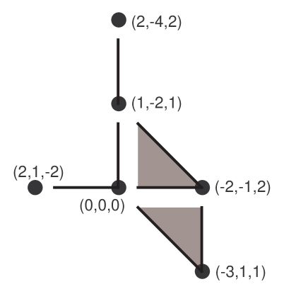
Figure 3.2: Lemma 3.1 applied to Example 1.6

Example 3.3.

Let $C_{\xi}$ be as in Example 1.6 and Figure 1.5. We may take $\bar{C}$ to be the vertex $\{0\}$; the edges $\{0,(2,1,-2)\}$, $\{0,(1,-2,1)\}$, and $\{0,(3,-1,-1)\}$; and the triangles $\{0,(2,1,-2),(3,-1,-1)\}$ and $\{0,(1,-2,1),(3,-1,-1)\}$. Then Lemma 3.1 gives the disjoint union illustrated in Figure 3.2.

We define another generating function that will be useful in the proof. Let

$$F_{\bar{C}}(\mathbf{x})=\frac{\sum_{s\in\bar{C}}(-1)^{\dim(s)}\mathbf{x}^{\max(s)}}{\prod(1-x_{i})},$$

where $\mathbf{x}=(x_{1},\ldots,x_{n})$. Then

$$f_{\bar{C}}(\mathbf{z})=F_{\bar{C}}(\mathbf{z}^{a_{1}},\mathbf{z}^{a_{2}},\ldots,\mathbf{z}^{a_{n}}).$$

Lemma 3.4.

Given $\xi\in\mathbb{Z}^{n}$ and $F_{\bar{C}}(\mathbf{x})$ as defined above, the coefficient of $\mathbf{x}^{\xi}$ in $F_{\bar{C}}(\mathbf{x})$ is

$$\sum_{s\in\bar{C}\cap C_{\xi}}(-1)^{\dim(s)}.$$

Proof.

For a given $s\in\bar{C}$, the term

$$\frac{(-1)^{\dim(s)}\mathbf{x}^{\max(s)}}{\prod(1-x_{i})}$$

will contribute $(-1)^{\dim(s)}\mathbf{x}^{\xi}$ if $\max(s)\leq\xi$, and otherwise it will contribute nothing. The proof follows, by the definition of $C_{\xi}$. ∎

Now we have the tools to prove Lemma 1.7.

Proof of Lemma 1.7:  Given a $L$-invariant simplicial complex, $C$, fix $b\in\mathbb{Z}^{d}$. Take a particular $\xi_{0}\in\mathbb{Z}^{n}$ such that $A\xi_{0}=b$. Then all $\xi\in\mathbb{Z}^{n}$ such that $A\xi=b$ are given by $\xi_{0}-\ell$, for $\ell\in L$. Let $d_{b}=\text{EC}(C_{\xi_{0}}).$ We want to show that the coefficient of $\mathbf{z}^{b}$ in $f_{\bar{C}}(\mathbf{z})$ is $d_{b}$. Since $f_{\bar{C}}(\mathbf{z})=F_{\bar{C}}(\mathbf{z}^{a_{1}},\mathbf{z}^{a_{2}},\ldots,\mathbf{z}^{a_{n}})$,

$$\text{the coefficient of }\mathbf{z}^{b}\text{ in }f_{\bar{C}}(\mathbf{z}) =\sum_{\xi\in\mathbb{Z}^{n}:\ A\xi=b}\text{the coefficient of }\mathbf{x}^{\xi}\text{ in }F_{\bar{C}}(\mathbf{x})$$

$$=\sum_{\ell\in\Lambda}\text{the coefficient of }\mathbf{x}^{\xi_{0}-\ell}\text{ in }F_{\bar{C}}(\mathbf{x})$$

$$=\sum_{\ell\in\Lambda}\sum_{\genfrac{}{}{0.0pt}{}{s^{\prime}\in}{\bar{C}\cap C_{\xi_{0}-\ell}}}(-1)^{\dim(s^{\prime})}\text{ (by Lemma \ref{CoeffF})}$$

$$=\sum_{\genfrac{}{}{0.0pt}{}{s\in C_{\xi_{0}},}{\ell:\ s-\ell\in\bar{C}}}(-1)^{\dim(s-\ell)}\text{ (by Lemma \ref{Union})}$$

$$=\sum_{s\in C_{\xi_{0}}}(-1)^{\dim(s)}$$

$$=d_{b}.$$

We have proven that, for all $b$, the coefficient of $z^{b}$ is the same in $\sum d_{b}\mathbf{z}^{b}$ and in $f_{\bar{C}}(\mathbf{z})$, and the proof follows. $\Box$

4 The Neighborhood Complex

Assume that $\Lambda$ is a generic lattice such that $A\lambda=0$ for all $\lambda\in\Lambda$ (we will deal with the nongeneric case in Section 5), and let $S$ be the neighborhood complex, as defined in Section 1. In this section, we will prove Theorems 1.3 and 1.4. First we will examine $S$ and the subcomplexes $S_{\xi}$ (the complex of $s\in S$ such that $\max(s)\leq\xi$). Our goal is to prove the following lemma.

Lemma 4.1.

Given $S$ as above, for $\xi\in\mathbb{Z}^{n}$, if $S_{\xi}\neq\emptyset$, then EC$(S_{\xi})=1$.

We will prove this lemma by giving a geometric realization of the $S_{\xi}$ and then using properties of this realization to compute the Euler characteristic. We will use a construction from [1], where the authors prove that a particular complex (the neighborhood complex with ideal vertices included) is homeomorphic to $\mathbb{R}^{m-1},$ where $m=\dim(\Lambda)$. In fact, the $S_{\xi}$ also have a nice topological property: they are contractible (this is shown in [5]). Contractibility implies that the Euler characteristic is 1 (this can be seen by applying standard facts from the homology of CW-complexes, see, for example, Theorem IX.4.4 of [10]), but here we will find EC($S_{\xi}$) directly and geometrically. Bayer and Sturmfels [6] also use a very similar construction to analyze their hull complex.

For purposes of exposition, we will present lemmas in a different order from how they are proved. The structure of the proof of Lemma 4.1 is: Lemma 4.7 and Lemma 4.6 imply Lemma 4.3, and then Lemma 4.2 and Lemma 4.3 imply Lemma 4.1.

Let $X=\{x^{1},x^{2},\ldots,x^{m}\}$, with $x^{i}\in\mathbb{R}^{n}$, be given. We define the complex $C(X)$ on the vertices $X$ to be the $s\subset X$ such that there is no $x\in X$ with $x<\max(s)$. $C(X)$ is a simplicial complex. We first prove the following lemma.

Lemma 4.2.

For $\xi\in\mathbb{Z}^{n}$, if $X=\{x\in\Lambda:\ x\leq\xi\}$, then $S_{\xi}=C(X)$.

Proof.

Suppose $s=\{\lambda^{1},\lambda^{2},\ldots,\lambda^{k}\}\in S_{\xi}$. Then $\lambda_{1},\ldots,\lambda_{k}\leq\xi$ and for no $\lambda\in\Lambda$ is $\lambda<\max(s)$. Therefore for no $x\in X$ is $x<\max(s)$ (since $X\subset\Lambda$), and so $s\in C(X)$.

Conversely, suppose $s=\{\lambda^{1},\lambda^{2},\ldots,\lambda^{k}\}\in C(X)$. Then $\lambda_{1},\ldots,\lambda_{k}\leq\xi$ and for no $x\in X$ is $x<\max(s)$. Suppose (seeking a contradiction) that $\lambda<\max(s)$ for some $\lambda\in\Lambda$. Then for each $i$ there is a $j$ such that

$$\lambda_{i}<\lambda^{j}_{i}\leq\xi_{i}.$$

But then $\lambda<\xi$ and so $\lambda\in X$, contradicting that for no $x\in X$ is $x<\max(s)$. Therefore, for no $\lambda\in\Lambda$ is $\lambda<\max(s)$, and so $s\in S_{\xi}$. ∎

We say that $X$ is generic if, whenever there is some $x^{1},x^{2}\in X$, with $x^{1}\neq x^{2}$ but $x^{1}_{i}=x^{2}_{i}$ for some $i$, then there is an $x\in X$ with $x<\max(x^{1},x^{2})$. This definition is slightly more complicated than for a lattice, because $X$ need not be lattice invariant. Then Lemma 4.1 will follow from Lemma 4.2, and the following lemma.

Lemma 4.3.

If $X=\{x^{1},x^{2},\cdots,x^{m}\}$ is generic and $C(X)$ is defined as above, then EC$\big{(}C(X)\big{)}=1$.

To prove this lemma, we follow the method of [1] and construct a polyhedron $P_{t}$ from the points $x^{1},x^{2},\ldots,x^{m}$, as follows. Given $t\geq 0$, define $E_{t}:\ \mathbb{R}^{n}\rightarrow\mathbb{R}^{n}$ by

$$E_{t}(x)=\mathbf{e}^{tx}=(e^{tx_{1}},e^{tx_{2}},\ldots,e^{tx_{n}}),$$

where $x=(x_{1},x_{2},\ldots,x_{n})$. Now we define

$$P_{t}=\mathbb{R}^{n}_{\geq 0}+\text{conv}\{E_{t}(x^{1}),E_{t}(x^{2}),\ldots,E_{t}(x^{m})\},$$

where $X=\{x^{1},x^{2},\ldots,x^{m}\}$.

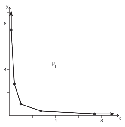
Figure 4.4: Example 4.5, $P_{1}$, with $X=\{-2,-1,0,1,2\}$

Example 4.5.

Let $X=\{-2,-1,0,1,2\}$. Then Figure 4.4 illustrates $P_{1}$.

The polyhedron $P_{t}$ has the following useful property.

Lemma 4.6.

There exists a sufficiently large $t$ such that, if $s\subset X$ with $s=\{s^{1},s^{2},\ldots,s^{k}\}$, then $s\in C(X)$ if and only if conv$\{E_{t}(s^{1}),E_{t}(s^{2}),\ldots,E_{t}(s^{k})\}$ is a face of $P_{t}$.

Proof.

The proof is very similar to the proof of Theorem 2 of [1]. We won’t go through the details. ∎

In Example 4.5 (see Figure 4.4), this lemma tells us that $C(X)$ has vertices $-2,-1,0,1,2$, and edges $\{-2,-1\},\{-1,0\},\{0,1\},\{1,2\}$, as we would expect. In general, Lemma 4.6 gives a geometric realization of $C(X)$ in $\mathbb{R}^{n}$. In fact, as shown in Theorem 2 of [1], if we take $X$ to be the (infinite) set $\Lambda$, $P_{t}$ gives a geometric realization of $S$, the entire neighborhood complex.

Now pick a sufficiently large $t$ such that Lemma 4.6 holds. Then the simplices in $C(X)$ are exactly the bounded faces of $P_{t}$. Then Lemma 4.3 (and hence Lemma 4.1) follows from the following lemma.

Lemma 4.7.

Let $P$ be an unbounded polyhedron in $\mathbb{R}^{n}$. Let $\mathcal{F}$ be the collection of bounded faces of $P$. Then

$$\text{EC}(\mathcal{F})=\sum_{F\in\mathcal{F}}(-1)^{\dim(F)}=1.$$

Proof.

Choose a half-space $H_{+}$ such that $H_{+}$ contains all of the bounded faces of $P$ in its interior and such that $P^{\prime}=P\cap H_{+}$ is bounded. Let $\mathcal{F}^{\prime}$ be the collection of faces of $P^{\prime}$. We know

$$\sum_{F^{\prime}\in\mathcal{F}^{\prime}}(-1)^{\dim(F^{\prime})}=1+(-1)^{n-1}.$$

This is the Euler-Poincaré formula, and it can be seen combinatorially (see, for example, Corollary VI.3.2 of [2]), or it can be seen from the fact that the complex $\mathcal{F}^{\prime}$ is homeomorphic to an $n-1$ sphere (and then applying standard facts from the homology of CW-complexes, see, for example, Theorem IX.4.4 of [10]). Let $H$ be the hyperplane which is the boundary of $H_{+}$. The faces of $P^{\prime}$ fall into $4$ categories:

1. $\mathcal{F}$, the bounded faces of $P$,
   

2. The face $P\cap H$,
   

3. $F\cap H_{+}$, where $F$ is an unbounded face of $P$, and
   

4. $F\cap H$, where $F$ is an unbounded face of $P$.
   

There is a bijective correspondence between the last two categories, mapping a face $F$ from category $3$ of dimension $k$ to $F\cap H$, a face from category $4$ of dimension $k-1$. Therefore, in $\sum_{F^{\prime}\in\mathcal{F}^{\prime}}(-1)^{\dim(F^{\prime})}$, these two categories will exactly cancel each other, and so we have

$$1+(-1)^{n-1}=\sum_{F^{\prime}\in\mathcal{F}^{\prime}}(-1)^{\dim(F^{\prime})}=\Big{[}\sum_{F\in\mathcal{F}}(-1)^{\dim(F)}\Big{]}+(-1)^{n-1}+0.$$

The lemma follows. ∎

Now we are ready to prove Theorems 1.3 and 1.4 (in the generic case).

Proof of Theorem 1.3: Let $\Lambda=L=\{\lambda\in\mathbb{Z}^{d}:\ A\lambda=0\}$, and let $S$ be the neighborhood complex on $\Lambda$. Take a particular $\xi_{0}\in\mathbb{Z}^{n}$ such that $A\xi_{0}=b$, and let $d_{b}=\text{EC}(S_{\xi_{0}})$. We want to show that

$$f_{\bar{S}}(\mathbf{z})=\sum_{b\in G}\mathbf{z}^{b},$$

and by Lemma 1.7 we know that

$$f_{\bar{S}}(\mathbf{z})=\sum_{b\in\mathbb{Z}^{d}}d_{b}\mathbf{z}^{b}.$$

By Lemma 4.1, we know that $d_{b}=1$ if and only if $S_{\xi_{0}}$ is nonempty (and $d_{b}=0$ otherwise), so it suffices to show that $S_{\xi_{0}}$ is nonempty if and only if $b\in G$.

Indeed, if $\{\lambda\}\in S_{\xi_{0}}$, for some $\lambda\in\Lambda$, then $\lambda\leq\xi_{0}$ and so $\xi_{0}-\lambda\geq 0$. Then, since $A\cdot(\xi_{0}-\lambda)=b-0=b$ with $\xi_{0}-\lambda\geq 0$, we have that $b\in G$. Conversely, if $b\in G$, then there is some $\xi\geq 0$ such that $A\xi=b$. Then $\xi_{0}-\xi\leq\xi_{0}$, and $A\cdot(\xi_{0}-\xi)=b-b=0$, so $\xi_{0}-\xi\in\Lambda$ and $\{\xi_{0}-\xi\}\in S_{\xi_{0}}$. The proof follows. $\Box$

Proof of Theorem 1.4: Let $\Lambda$ be a lattice in $\mathbb{Z}^{n}$ such that $A\lambda=0$, for all $\lambda\in\Lambda$, and let $S$ be the neighborhood complex defined on $\Lambda$. Recall that, for $b\in\mathbb{Z}^{n}$, we define $T_{b}=\{\xi\in\mathbb{Z}^{n}:\ \xi\geq 0\text{ and }A\xi=b\}$, we define an equivalence relation on $T_{b}$ by $\xi\sim\eta$ if and only if $\xi-\eta\in\Lambda$, and we define $c_{b}$ to be the number of equivalence classes in $T_{b}$. To use Lemma 1.7, we must have a lattice invariant neighborhood complex on all of $L=\{\ell\in\mathbb{Z}^{n}:\ A\ell=0\}$. Let $\bar{L}$ be a set of distinct representatives of $L$ modulo $\Lambda$, and define $C$ to be the disjoint union

$$C=\bigcup_{\ell\in\bar{L}}S+\ell.$$

$C$ is an $L$-invariant complex, and we can choose $\bar{C}$ and $\bar{S}$ (representatives of $C$ modulo $L$ and $S$ modulo $\Lambda$, respectively) such that $\bar{C}=\bar{S}$. By Lemma 1.7, we know

$$f_{\bar{S}}(\mathbf{z})=f_{\bar{C}}(\mathbf{z})=\sum_{b\in\mathbb{Z}^{d}}d_{b}\mathbf{z}^{b},$$

where $d_{b}=\text{EC}(C_{\xi}),\text{ for some (any) }\xi\text{ such that }A\xi=b$. Therefore we need to show that $c_{b}=d_{b}$, for all $b\in\mathbb{Z}^{n}$.

Fix a $\xi_{0}$ such that $A\xi_{0}=b$. We claim that

$$C_{\xi_{0}}=\bigcup_{\ell\in\bar{L}}(S_{\xi_{0}+\ell}-\ell),$$

where the union is disjoint. Indeed, if $s=\{\ell^{1},\ell^{2},\ldots,\ell^{k}\}\in C_{\xi_{0}}$, then, for each $i$, $\ell^{i}\leq\xi_{0}$. Take $\ell\in\bar{L}$ such that $s+\ell\in S$. Then $\ell^{i}+\ell\leq\xi_{0}+\ell$, and so $s+\ell\in S_{\xi_{0}+\ell}$ and $s\in S_{\xi_{0}+\ell}-\ell.$ Conversely, if $s=\{\ell^{1},\ell^{2},\ldots,\ell^{k}\}\in S_{\xi_{0}+\ell}-\ell,$ then $\ell^{i}+\ell\leq\xi_{0}+\ell$, for all $i$. Therefore, $\ell^{i}\leq\xi_{0}$, and so $s\in C_{\xi_{0}}$. In addition, the union is disjoint, because $S_{\xi+\ell}+\ell\subset S+\ell$, which are themselves disjoint.

Since we have written $C_{\xi_{0}}$ as a disjoint union, we have

$$\text{EC}(C_{\xi_{0}})=\sum_{\ell\in\bar{L}}\text{EC}(S_{\xi_{0}+\ell}).$$

Since EC$(S_{\xi_{0}+\ell})=1$ if $S_{\xi_{0}+\ell}\neq\emptyset$, by Lemma 4.1, and EC$(S_{\xi_{0}+\ell})=0$ if $S_{\xi_{0}+\ell}=\emptyset$, we have

$$\text{EC}(C_{\xi_{0}})=\#\{\ell\in\bar{L}:\ S_{\xi_{0}+\ell}\neq\emptyset\}.$$

Therefore, to prove Theorem 1.4, we must show that the number of nonempty $S_{\xi_{0}+\ell}$ is the number, $c_{b}$, of equivalence classes of $T_{b}$.

For $\xi,\eta\in T_{b}$, $\xi\sim\eta$ if and only if $\xi-\eta\in\Lambda$, which happens if and only if $\xi$ and $\eta$ are in the same coset $\xi_{0}+(\ell+\Lambda)$, for some $\ell\in\bar{L}$. Then the equivalence classes of $T_{b}$ are exactly the $\big{(}\xi_{0}+(\ell+\Lambda)\big{)}\cap\mathbb{Z}^{n}_{\geq 0}$ which are nonempty. But $\lambda\in\Lambda$ is such that $\xi_{0}+(\ell+\lambda)\geq 0$ if and only if $-\lambda\leq\xi_{0}+\ell$, which happens if and only if $\{-\lambda\}\in S_{\xi_{0}+\ell}$. Therefore $S_{\xi_{0}+\ell}$ is nonempty if and only if $\big{(}\xi_{0}+(\ell+\Lambda)\big{)}\cap\mathbb{Z}^{n}_{\geq 0}$ is a nonempty equivalence class of $T_{b}$. The proof of Theorem 1.4 follows. $\Box$

5 The Non-generic Case

The strategy we follow is to perturb the elements of $\Lambda$ so that no two have any coordinate that is the same. Then we will be in the generic case and can apply the lemmas of the last section.

We call $\varphi:\Lambda\rightarrow\mathbb{R}^{n}$ a proper perturbation if the following 3 conditions hold:

1. If $x\neq y$, then $[\varphi(x)]_{i}\neq[\varphi(y)]_{i}$,

2. If $[\varphi(x)]_{i}<[\varphi(y)]_{i}$, then $x_{i}\leq y_{i}$, and

3. If $[\varphi(x)]_{i}<[\varphi(y)]_{i}$, then $[\varphi(x+\lambda)]_{i}<[\varphi(y+\lambda)]_{i}$ for all $\lambda\in\Lambda$.

The first condition insures that we will be in the generic case, the second insures that the perturbation only “breaks ties” and doesn’t change the natural ordering, and the third condition will be needed to prove that the neighborhood complex is lattice invariant.

To prove that proper perturbations exist, we will construct an example of one.

Example 5.1.

This example corresponds to the lexicographical tie-breaking rule used in [12]. Given an integer $i$, let $f_{i}:\mathbb{Z}\rightarrow\mathbb{R}$ be a function such that

1. $f_{i}$ is strictly increasing,

2. $f_{i}(0)=0$ (an hence $f_{i}(x)<0$ if $x<0$), and

3. if $\lvert x\rvert>0$ (hence $\lvert x\rvert\geq 1$), then $\frac{1}{2^{2i}}\leq\lvert f_{i}(x)\rvert<\frac{1}{2^{2i-1}}$.

For example, $f_{i}$ could be an appropriate rescaling of $\arctan(x)$. Now define $\varphi:\Lambda\rightarrow\mathbb{R}^{n}$ by

$$\varphi(x)=x+(x_{1}f_{1}(x_{1})+x_{2}f_{2}(x_{2})+\cdots+x_{n}f_{n}(x_{n}))\cdot\mathbf{1},$$

where $\mathbf{1}$ is the $n$-vector of ones. One can check that $\varphi$ is a proper perturbation.

Given a proper perturbation $\varphi$, we can now define the neighborhood complex, $S$, on the vertices $\Lambda$, by saying $s=\{\lambda^{1},\lambda^{2},\ldots,\lambda^{k}\}$ is in $S$ if and only if for no $\lambda\in\Lambda$ is $\varphi(\lambda)<\max(\varphi(s))$, where $\varphi(s)=\{\varphi(\lambda^{1}),\varphi(\lambda^{2}),\ldots,\varphi(\lambda^{k})\}$. $S$ may be different for different $\varphi$, but many properties (including Theorems 1.3 and 1.4) hold regardless of the choice of $\varphi$. The following lemma shows that $S$ is invariant under lattice translations, and so $f_{\bar{S}}(\mathbf{z})$, as defined in Section 1, makes sense.

Lemma 5.2.

If $\varphi$ is a proper perturbation, then the neighborhood complex $S$, as defined above, is lattice invariant.

Proof.

Given $\lambda\in\Lambda$, we have the following chain of implications:

$$s =\{\lambda^{1},\lambda^{2},\ldots,\lambda^{k}\}\in S$$

$$\Rightarrow\text{for no }\lambda^{\prime}\in\Lambda\text{ is }\varphi(\lambda^{\prime})<\max(\varphi(s))$$

$$\Rightarrow\text{given }\lambda^{\prime}\in\Lambda,\ \exists i\text{ such that }\forall j\ [\varphi(\lambda^{\prime})]_{i}\geq[\varphi(\lambda^{j})]_{i}$$

$$\Rightarrow\text{given }\lambda^{\prime}\in\Lambda,\ \exists i\text{ such that }\forall j\ [\varphi(\lambda^{\prime}+\lambda)]_{i}\geq[\varphi(\lambda^{j}+\lambda)]_{i}$$

(by Property 3 of proper perturbations)

$$\Rightarrow\text{for no }\lambda^{\prime}\in\Lambda\text{ is }\varphi(\lambda^{\prime}+\lambda)<\max(\varphi(s+\lambda))$$

$$\Rightarrow s+\lambda\in S.$$

∎

Given $\xi\in\mathbb{Z}^{n}$, we define $S_{\xi}$ as in Section 1, that is, $S_{\xi}$ is the complex of all $s\in S$ such that $\max(s)\leq\xi$. For generic $X\subset\mathbb{R}^{n}$, define $C(X)$ as in Section 4, that is, $C(X)$ is the simplicial complex of $s\subset X$ such that there is no $x\in X$ with $x<\max(s)$. We mimic Lemma 4.2.

Lemma 5.3.

If $\varphi$ is a proper perturbation, if $\xi\in\mathbb{Z}^{n}$ is given, and if $Y=\{y\in\Lambda:\ y\leq\xi\}$, then $\varphi(S_{\xi})=C(\varphi(Y))$ (and hence $S_{\xi}$ is isomorphic to $C(\varphi(Y))$).

Proof.

Suppose $s=\{\lambda^{1},\lambda^{2},\ldots,\lambda^{k}\}\in S_{\xi}$. Then $\lambda^{1},\ldots,\lambda^{k}\leq\xi$ and for no $\lambda\in\Lambda$ is $\varphi(\lambda)<\max(\varphi(s))$. Therefore for no $y\in Y$ is $\varphi(y)<\max(\varphi(s))$ (since $Y\subset\Lambda$), and so $\varphi(s)\in C(\varphi(Y))$.

Conversely, suppose $\varphi(s)\in C(\varphi(Y))$, with $s=\{\lambda^{1},\lambda^{2},\ldots,\lambda^{k}\}$. Then $\lambda^{1},\ldots,\lambda^{k}\leq\xi$ and for no $y\in Y$ is $\varphi(y)<\max(\varphi(s))$. Suppose (seeking a contradiction) that $\varphi(\lambda)<\max(\varphi(s))$ for some $\lambda\in\Lambda$. Then for each $i$ there is a $j$ such that

$$[\varphi(\lambda)]_{i}<[\varphi(\lambda^{j})]_{i}.$$

Therefore $\lambda_{i}\leq\lambda^{j}_{i}$, by Property 2 of proper perturbations, and so

$$\lambda_{i}\leq\lambda^{j}_{i}\leq\xi_{i}.$$

But then $\lambda\leq\xi$ and so $\lambda\in Y$, contradicting that for no $y\in Y$ is $\varphi(y)<\max(\varphi(s))$. Therefore, for no $\lambda\in\Lambda$ is $\varphi(\lambda)<\max(\varphi(s))$, and so $s\in S_{\xi}$. ∎

In particular, this lemma, together with Lemma 4.3, implies that

$$\text{EC}(S_{\xi})=\text{EC}\big{(}C(\varphi(Y))\big{)}=1$$

whenever $S_{\xi}$ is nonempty. The proofs of Theorems 1.3 and 1.4 in the non-generic case are now identical to their proofs in the generic case (see Section 4).

Cowles Foundation for Research in Economics, Yale University, New Haven, Connecticut 06511
herbert.scarf@yale.edu

Department of Mathematics, University of Michigan, Ann Arbor, Michigan 48109
kmwoods@umich.edu

References

- [1] I. Bárány, H.E. Scarf, and D. Shallcross: The topological structure of maximal lattice free convex bodies: the general case, Mathematical Programming 80 (1998), 1-15.
- [2] A. Barvinok: A Course in Convexity, Graduate Studies in Mathematics 54, Amer. Math. Soc., Providence (2002).
- [3] A. Barvinok and J. Pommersheim: An algorithmic theory of lattice points in polyhedra. New Perspectives in Geometric Combinatorics, MSRI Publications 38 (1999), 91-147.
- [4] A. Barvinok and K. Woods, Short rational generating functions for lattice point problems, Journal of the AMS 16 (2003), 957-979.
- [5] D. Bayer, I. Peeva, B. Sturmfels: Monomial resolutions, manuscript.
- [6] D. Bayer and B. Sturmfels: Cellular resolutions of monomial modules, J. Reine Angew. Math. 502 (1998), 123-140.
- [7] G. Denham: The Hilbert series of a certain module, manuscript (1996).
- [8] J. Herzog: Generators and relations of abelian semigroups and semigroup rings, Manuscripta Math. 3 (1970), 175-193.
- [9] L. Lovász: Geometry of numbers and integer programming, in: M. Iri and K. Tanabe, eds., Mathematical Programming: Recent Developments and Applications, Kluwer, Norwell, MA (1989), 177-210.
- [10] W.S. Massey: A Basic Course in Algebraic Topology, Graduate Texts in Mathematics 127, Springer-Verlag, New York (1991).
- [11] I. Peeva and B. Sturmfels, Generic lattice ideals, Journal of the AMS 11 (1998), 363-373.
- [12] H. E. Scarf: Production sets with indivisibilities, part II: The case of two activities, Econometrica 49(2) (1981), 395-423.
- [13] H. E. Scarf, Test sets for integer programs, Math. Programming, Series B 79 (1997), 355-368.
- [14] H.E. Scarf and D. Shallcross: The Frobenius problem and maximal lattice free bodies, Math. Op. Res. 18(3) (1993), 511-515.
- [15] D. Shallcross: Neighbors of the origin for four by three matrices: Math. Op. Res. 17(3) (1992), 608-614.