Ricci Tensors with Rotational Symmetry on ${\mathbb{R}}^{n}$

Abstract.

In this paper is considered the differential equation $Ric(g)=T$, where $Ric(g)$ is the Ricci tensor of the metric $g$ and $T$ is a rotational symmetric tensor on ${\mathbb{R}}^{n}$. A new, geometric, proof of the existence of smooth solutions of this equation, based on qualitative theory of implicit differential equations, is presented here. This result was obtained previously by DeTurck and Cao in 1994.

1. Introduction

In this paper will be considered a particular case of the second order partial differential equation

$$Ric(g)=T,$$ (1)

where $g$ is a Riemannian metric in a manifold $\mathbb{M}^{n}$, $Ric(g)$ is the Ricci tensor of $g$ and $T$ is a given symmetric tensor of second order. This equation is of physical significance in field theory, see chapter XI of [16] and chapter 18 of [19]. For example, the Einsten’s gravitational equations, the Maxwell’s equations of electromagnetic fields and the Euler equations for fluids are related to equation 1. The tensor $T$ is interpreted physically as the stress-energy tensor due to the presence of matter.

DeTurck showed that if $M$ is a surface then the equation $Ric(g)=T$ can be solved locally if $T=\rho\gamma$ where $\rho$ is a smooth real function and $\gamma$ is a positive definite tensor, see [4].

Also DeTurck showed that in dimension 3 or more the problem $Ric(g)=T$, with $T$ non singular, has local solution in the smooth or analytic category and that for $T=x_{1}dx_{1}^{2}+dx_{2}^{2}+\cdots+dx_{n}^{2}$, singular at $x_{1}=0$, then the problem has no local solution near $x_{1}=0$, see [5].

Recently, DeTurck and Goldschmidt studied the equation 1 with $T$ singular, but of constant rank. A detailed analysis of integrability conditions for local solvability was obtained. Also the authors obtained various results of existence of local solutions, under additional hypothesis, see [7].

In this work will be considered the Ricci equation $Ric(g)=T_{S}$, where $g=e^{2f}g_{0}$ is a conformal deformation of the canonical metric $g_{0}=dr^{2}+r^{2}d\Theta^{2}$ of $\mathbb{R}^{n}$ and $T_{S}$ is a given tensor with $SO(n)$ rotational symmetry. This problem was considered previously by DeTurck and Cao, [6]. They obtained local solutions near the origin $0$.

This paper provides a new proof of existence and unicity, up to homothety, of smooth local solutions near the origin of $\mathbb{R}^{n}$ for the equation $Ric(g)=T_{S}$.

In the paper by DeTurck and Cao, [6], no explicit statement about the smoothness of the metric $g$ at $0$ is presented.

This paper is organized as follows. In section 2 the definition of Ricci tensor is recalled and the problem $Ric(g)=T$ is formulated. In section 3 the main results of this work are stated in proved. In section 4 we give an example of a metric $g$ with rotational symmetry in $\mathbb{R}^{n}$ and the associated Ricci tensor is calculated explicitly. Finally in section 5 some general problems are stated.

2. Preliminaries

On a n-dimensional Riemannian manifold $(M,g)$ the associated Riemann or curvature tensor $R=R(g)$ is given, in a local chart, by the coefficients $R_{ijkl}$. The following relations hold.

$$R_{ijkl} =R_{klij}$$

$$R_{ijkl}+R_{iljk}+R_{iklj} =0$$

$$\nabla_{m}R_{ijkl}+\nabla_{k}R_{ijlm}+\nabla_{l}R_{ijmk} =0$$

This space of coefficients has dimension $n^{2}(n^{2}-1)/12$.

The contraction $R_{ik}=g^{jl}R_{ijkl}$ of the curvature tensor is the called the Ricci tensor, see [2] and [15]. So, for each $p\in M$ the Ricci tensor is a symmetric bilinear form $Ric(g):T_{p}M\times T_{p}M\to\mathbb{R}$ and therefore the dimension of the space of coefficients $R_{ik}$ is equal to $n(n+1)/6$. The Ricci curvature in the direction $X=\{X_{i}\}$ is $R_{ij}X_{i}X_{j}$ and $g^{ij}R_{ij}$ is called the scalar curvature.

In local coordinates the Ricci tensor is given by:

$$R_{ij}= \frac{1}{2(n-1)}g^{kl}[\frac{\partial^{2}g_{jl}}{\partial x^{i}\partial x^{k}}+\frac{\partial^{2}g_{ik}}{\partial x^{j}\partial x^{l}}-\frac{\partial^{2}g_{kl}}{\partial x^{i}\partial x^{j}}-\frac{\partial^{2}g_{ij}}{\partial x^{k}\partial x^{l}}]$$ (2)

$$+ \frac{1}{n-1}g^{kl}g_{pq}[\Gamma_{ik}^{p}\Gamma_{jl}^{q}-\Gamma_{ij}^{p}\Gamma_{kl}^{q}]$$

$$= \frac{\partial\Gamma_{ij}^{s}}{\partial x^{s}}-\frac{\partial\Gamma_{is}^{s}}{\partial x^{j}}+\Gamma_{ij}^{s}\Gamma_{st}^{t}-\Gamma_{it}^{s}\Gamma_{sj}^{t}$$

where,

$$\Gamma_{ij}^{l}=\frac{1}{2}g^{kl}[\frac{\partial g_{jk}}{\partial x^{i}}+\frac{\partial g_{ik}}{\partial x^{j}}-\frac{\partial g_{ij}}{\partial x^{k}}]$$ (3)

are the Christoffel symbols of the metric $g$.

In the two dimensional situation $R_{1212}=\mathcal{K}$ is the Gaussian curvature and it is the only non zero coefficient of both tensors.

In the three dimensional case there exists an algebraic relation between $R(g)$ and $Ric(g)$ which is given by:

$$R_{ijkl}=g_{ik}R_{jl}-g_{il}R_{jk}-g_{jk}R_{il}+g_{jl}R_{ik}-\frac{1}{2}R(g_{ik}g_{jl}-g_{il}g_{jk}).$$

Here $R=g^{ik}R_{ik}$ is the scalar curvature, see [12] and [17].

For $n\geq 4$, in general, the Ricci tensor does not determine the Riemannian curvature tensor.

Also the following holds.

Let $M\subset\mathbb{R}^{n+1}$ be a hypersurface with second fundamental form $h$ and $\{X_{1},\cdots,X_{n}\}$ be an orthonormal frame given by the principal directions $X_{i}$. It follows that the principal curvatures are given by $h_{i}=h(X_{i},X_{i})$ and according to [17] the Riemman tensor is given by :

$$R_{ijkl}= h(X_{i},X_{k})h(X_{j},X_{l})-h(X_{j},X_{k})h(X_{i},X_{l})$$

$$= h_{i}h_{j}(\delta_{ik}\delta_{jl}-\delta_{jk}\delta_{il}).$$

So the Ricci tensor is given by

$$R_{ij}=\delta_{ij}[h_{i}(h_{1}+\cdots+h_{n})-h_{i}^{2}].$$

The scalar curvature is equal to

$$R=(\sum_{i=1}^{n}h_{i})^{2}-\sum_{i=1}^{n}h_{i}^{2}.$$

In this paper we will consider the following restricted problem, studied by Cao and DeTurck, [6].

Problem:Given a smooth rotational symmetric tensor $T$ on ${\mathbb{R}}^{n}$, determine, if it exists, a smooth metric $g$ such that

$$Ric(g)=T.$$ (4)

3. Rotationally Symmetric Tensors

Consider a tensor $T$ on the n-dimensional Euclidean space $\mathbb{R}^{n}$ symmetric with respect to the orthogonal group $SO(n)$; that is $\gamma*T=T$ for every $\gamma\in SO(n)$. These tensors will be referred to as rotationally symmetric.

Under the hypothesis of non singularity of $T$, the following lemma was proved in [6].

Lemma 1.

Let $T=\varphi(t)dt^{2}+t^{2}\psi(t)d\Theta^{2}$, $t\in\mathbb{R}_{+}$ and $\Theta\in{\mathbb{S}}^{n-1}$, a smooth, nonsingular and rotationally symmetric tensor on $\mathbb{R}^{n}$. Then $T$ is either positive or negative definite everywhere. Moreover $\varphi(0)=lim_{t\to 0}\psi(t)$.

Consider also a smooth rotationally symmetric metric $g,$ expressed in spherical coordinates $(r,\Theta)=(r,\theta_{1},\cdots,\theta_{n-1})$, as

$$g=2e^{f(t)}[r^{\prime}(t)dt^{2}+r(t)^{2}d\Theta^{2}].$$ (5)

where, $r(0)=0$, $r^{\prime}(0)=1$ and $r^{\prime}(t)>0$ for all $t>0$.

The Ricci tensor of $g$ defined by equation 5, see [6], is given by:

$$Ric(g)=\alpha(r)dr^{2}+r^{2}\beta(r)d\Theta^{2}$$ (6)

where,

$$\alpha(r) =-(n-1)[f_{rr}+\frac{f_{r}}{r}]$$

$$\beta(r) =-[f_{rr}+(2n-3)\frac{f_{r}}{r}+(n-2)(f_{r})^{2}]$$

$$f_{r} =f^{\prime}(t)/r^{\prime}(t)\;\;\;\;\text{ and}\;\;\;\;f_{rr}=f^{\prime}_{r}(t)/r^{\prime}(t).$$

Therefore the equation $Ric(g)=T$ is equivalent to the following.

$$t^{2}\psi=[\frac{\varphi}{n-1}(\frac{r}{r^{\prime}})^{2}]-(n-2)[2rf_{r}+(rf_{r})^{2}].$$

If $\varphi\neq 0$ it follows that:

$$\frac{t^{2}\psi\varphi}{n-1}=[\frac{\varphi r}{(n-1)r^{\prime}}]^{2}-\frac{(n-2)}{n-1}\varphi[2rf_{r}+(rf_{r})^{2}]$$ (7)

In [6] the Ricci potential was defined as

$$w(t)=\frac{1}{2\pi}\int_{D_{t}}KdA_{g}.$$

Here $D_{t}=\{(s,\Theta)\in W:0\leq s\leq t\}$ and $W$ is a fixed two dimensional subspace of $\mathbb{R}^{n}$ and $K$ is the sectional curvature of $W$. The function $w$ is well defined since the metric $g$ is rotationally symmetric.

Lemma 2.

If $w$ is the Ricci potential of the rotationally symmetric metric $g=2e^{f(t)}[r^{\prime}(t)dt^{2}+r(t)^{2}d\Theta^{2}]$ then

$$w(t)= -rf_{r}=-\frac{r(t)}{r^{\prime}(t)}f^{\prime}(t)$$ (8)

$$w^{\prime}(t)= \frac{\varphi r}{(n-1)r^{\prime}}$$

Proof.

The sectional curvature of the plane $W$ is given by

$$K=-e^{-2f}[f_{rr}+\frac{f_{r}}{r}].$$

Therefore it follows that

$$w(t)=\frac{1}{2\pi}\int_{D_{t}}KdA_{g}=\frac{1}{2\pi}\int_{0}^{t}\int_{0}^{2\pi}K(t)r(t)e^{2f(t)}r^{\prime}(t)dt.$$

Then,

$$\frac{dw}{dt}= K(t)r(t)e^{f(t)}r^{\prime}(t)$$

$$= -[f_{rr}+\frac{f_{r}}{r}]r(t)r^{\prime}(t)$$

$$= -\frac{d}{dt}[rf_{r}].$$

As $w(0)=0$ and $r(0)=0$ it follows that $w(t)=-r(t)f_{r}(t)$. Differentiating the equation above it follows that

$$w^{\prime}(t)=-r^{\prime}f_{r}-rf_{rr}r^{\prime}=\frac{\varphi(t)r(t)}{(n-1)r^{\prime}(t)}.$$

∎

In terms of the Ricci potential $w$ it follows, from equation 7, the following implicit differential equation.

$$\left(\frac{dw}{dt}\right)^{2}=\frac{1}{n-1}[(n-2)\varphi(t)(w^{2}-2w)+t^{2}\varphi(t)\psi(t)]$$ (9)

Proposition 1.

The implicit differential equation 9 with $\varphi(0)=\psi(0)\neq 0$, has a unique local smooth solution, with initial condition $w(0)=w^{\prime}(0)=0$, defined in the interval $[0,\epsilon)$, such that $w^{\prime}(t)\varphi(0)>0$ for all $t\in(0,\epsilon)$.

Proof.

For $n=2$ the implicit differential equation 9 is equivalent to the ordinary differential equations $dw/dt=\pm t\sqrt{\varphi(t)\psi(t)}$. Direct integration leads to the result stated.

So we suppose $n>2$. Consider smooth extensions of $\varphi$ and $\psi$ for $t<0$ and the implicit surface

$${\mathcal{F}}(t,w,p)=\frac{1}{n-1}[(n-2)\varphi(t)(w^{2}-2w)+t^{2}\varphi(t)\psi(t)]-p^{2}\,\,=0,$$

where $p=\frac{dw}{dt}$.

Under the hypothesis above, we have $d{\mathcal{F}}(0)=[0\;\;\frac{n-2}{n-1}\varphi(0)\;\;0]\neq 0$, so ${\mathcal{F}}^{-1}(0)$ is locally a regular smooth surface near $0$.

Next we consider the smooth Lie-Cartan vector field

$$X={\mathcal{F}}_{p}\frac{\partial}{\partial t}+p{\mathcal{F}}_{p}\frac{\partial}{\partial w}-({\mathcal{F}}_{t}+p{\mathcal{F}}_{w})\frac{\partial}{\partial p},$$

defined in a tubular neighborhood of the surface ${\mathcal{F}}^{-1}(0)$ and tangent to it.

The projections of the integral curves of $X$ by $\pi(t,w,p)=(t,w)$ are the solutions of equation 9.

The origin $0$ is a singular point of $X$, isolated in ${\mathcal{F}}^{-1}(0),$ and

$$DX(0)=\begin{pmatrix}0&0&-2\\ 0&0&0\\ \frac{-2\varphi(0)\psi(0)}{n-1}&-2\frac{(n-2)\varphi^{\prime}(0)}{n-1}&2\frac{(n-2)\varphi(0)}{n-1}\end{pmatrix}$$

The non zero eigenvalues of $DX(0)$, $\lambda_{1}$ and $\lambda_{2}$ are the roots of

$$-\lambda^{2}+2\frac{(n-2)\varphi(0)}{n-1}\lambda+\frac{4\varphi(0)\psi(0)}{n-1}=0.$$

As $\lambda_{1}\lambda_{2}=-4\frac{\varphi(0)\psi(0)}{n-1}<0$, it follows that $0$ is a hyperbolic saddle point of $X|_{{\mathcal{F}}^{-1}(0)}$. Also the unstable and stable separatrices are transversal to the regular fold curve $\Sigma$, defined by $\Sigma=\{(t,w,p)|{\mathcal{F}}(t,w,p)={\mathcal{F}}_{p}(t,w,p)=0\}$.

Therefore the projections, by $\pi$, of the smooth stable and unstable separatrices of the hyperbolic singularity $0$ are smooth and quadratically tangent to $\pi(\Sigma)$. Direct calculation shows that $\pi(\Sigma)=\{(t,w(t),0):w(t)=\frac{\psi(0)}{n-1}\frac{t^{2}}{2}+\cdots\}$. The projections of the separatrices of the hyperbolic saddle will be called folded separatrices. The integral curves of $X$ and of their projections in the plane $(t,w)$ are as shown in the Figure 1 below. ∎

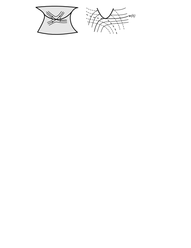
Figure 1. Folded saddle point

Remark 1.

The proposition 1 corresponds to Lemma 2.1 (also labelled Proposition 2.1) and Propositions 2.2 and 2.3 of [6]. In the mentioned paper there is no statement about the smoothness of the solution $w$ at $0$, the fixed point of the rotation group. We adopt to work in the $C^{\infty}$ category, but with the obvious changes the result is valid in the $C^{r}$, $r\geq 2$, category.

Remark 2.

The analysis above is similar to that carried out in the study of asymptotic lines near a parabolic curve, see [10].

Lemma 3.

Let $w$ be the smooth solution of equation (9). Consider the singular differential equation

$$(n-1) w^{\prime}r^{\prime}-\varphi r=0$$ (10)

$$r(0)= 0,\;\;r^{\prime}(0)=1$$

$$w(0)= \;w^{\prime}(0)=0,\;\;w^{\prime\prime}(0)=\frac{\varphi(0)}{n-1}$$

Then there exists a smooth solution $r=r(t)$ of equation (10) in a interval $[0,\epsilon)$.

Proof.

Let $r(t)=tR(t)$ and $w(t)=\frac{t^{2}}{2}W(t)$. Then it follows that the equation (10) is equivalent to the following equation

$$t\frac{dR}{dt}=\frac{\varphi R}{(n-1)(W+\frac{t}{2}W^{\prime})}-R$$ (11)

Therefore, the line $(0,R)$ is a normally hyperbolic set and, by Invariant Manifold Theory, [14], there exists a smooth solution $R(t)$ defined in a neighborhood of $0$ with initial condition $R(0)=1$. ∎

Lemma 4.

Let $w$ be the smooth solution of equation (9). Consider the singular differential equation

$$(n-1) w^{\prime}f^{\prime}+w\varphi=0$$ (12)

$$f(0)= 0,$$

$$w(0)= \;w^{\prime}(0)=0,\;\;w^{\prime\prime}(0)=\frac{\varphi(0)}{n-1}$$

Then there exists a smooth solution $f=f(t)$ of equation (12) in a interval $[0,\epsilon)$.

Proof.

The same argument as in the proof of lemma 3 works here. ∎

¿From proposition 1 and lemmas 3 and 4 follows the next proposition.

Proposition 2.

Let $T=\varphi(t)dt^{2}+t^{2}\psi(t)d\Theta^{2}$ be non singular everywhere and suppose $w$ is a solution of equation (9) such that $w(0)=w^{\prime}(0)$ and $w^{\prime}(t)\varphi(t)>0$ for $t>0$. Then the Ricci system $Ric(g)=T$ is solvable. In fact, $g=2e^{f(t)}[r^{\prime}(t)dt^{2}+r(t)^{2}d\Theta^{2}]$, where $r$ and $f$ are as stated, respectively, in lemmas 3 and 4.

Also formally we can write,

$$r(t)= t\text{ exp}\left(\int_{0}^{t}\left[\frac{\varphi(s)}{(n-1)w^{\prime}(s)}-\frac{1}{s}\right]ds\right),$$ (13)

$$f(t)= -\int_{0}^{t}w(s)\frac{r^{\prime}(s)}{r(s)}ds+c=-\int_{0}^{t}\frac{\varphi}{n-1}\frac{w}{w^{\prime}}ds+c.$$

Proof.

¿From lemma 2 it follows that $w(t)=-r(t)f_{r}(t)=-r(t)f^{\prime}(t)/r^{\prime}(t)$ and $w^{\prime}(t)=\varphi(t)r(t)/(n-1)r^{\prime}(t)$. From lemmas 3 and 4 follows that $r(t)$ and $f(t)$ are smooth solutions of these equations. Therefore, integration leads to the following result. ∎

Theorem 1.

Consider the smooth, nonsingular, rotationally symmetric tensor $T=\varphi(t)dt^{2}+t^{2}\psi(t)d\Theta^{2}$. Suppose that ${\mathcal{F}}^{-1}(0)$ is a regular surface for all $t\geq 0$ and $\frac{d}{dt}(t^{2}\psi(t))\varphi(t)\neq 0$, i.e., the set $\Sigma$, defined by $\Sigma=\{(t,w,p)|{\mathcal{F}}(t,w,p)={\mathcal{F}}_{p}(t,w,p)=0\}$ is a regular curve. Then $Ric(g)=T$ has a rotationally symmetric solution $g$ defined on all $\mathbb{R}^{n}$.

Proof.

The solution of the Ricci equation $Ric(g)=T$ is obtained from the stable or unstable separatrix of a hyperbolic saddle of $X$. This separatrix is defined until it reaches the boundary of a connected component of the set $\{(t,w,p)|\;{\mathcal{F}}(t,w,p)\geq 0\}$, which is, under the hypothesis above, the regular curve $\pi(\Sigma)$. The condition $\frac{d}{dt}(t^{2}\psi(t))\varphi(t)\neq 0$ means that the folded curve $\Sigma=\{(t,w,p):{\mathcal{F}}(t,w,p)={\mathcal{F}}_{p}(t,w,p)=0\}$ is a regular curve, with two connected components and that the vector field $X$ has no singular point outside $0$ on the connected component of $\pi(\Sigma)$ that contains $0$. Therefore, the folded separatrices of the saddle point $0$ of $X$ cannot reach the boundary of $\{(t,w,p)|\;{\mathcal{F}}(t,w,p)\geq 0\}$. If this occurs there would be a topological disk, bounded by a folded separatrix and by a connected component of the folded curve, foliated by regular curves transversal, outside $0$, to the folded curve. But this is impossible. ∎

4. Hypersurfaces with Rotational Symmetry

In this section we will calculated the Ricci tensor for a rotationally symmetric hypersurface of $\mathbb{R}^{n+1}$.

Let $\alpha:\mathbb{R}^{n}\to\mathbb{R}^{n+1}$ be an embedding with rotational symmetry, i.e, a graph of a function $h$, given by $\alpha(y_{1},\cdots,y_{n})=(y_{1},\cdots,y_{n},h(y_{1}^{2}+\cdots+y_{n}^{2}))$.

In spherical coordinates it follows that:

$\alpha(r,\theta_{1},\cdots,\theta_{n-1})=(y_{1},\cdots,y_{n},y_{n+1})$ where,

$$y_{1}= r\cos\theta_{1}\cdots\cos\theta_{n-1}$$ (14)

$$y_{2}= r\cos\theta_{1}\cdots\cos\theta_{n-2}\sin\theta_{n-1}$$

$$\cdots= \cdots$$

$$y_{n-1}= r\cos\theta_{1}\sin\theta_{2}$$

$$y_{n}= r\sin\theta_{1}$$

$$y_{n+1}= h(r^{2})$$

Therefore the first fundamental form of $\alpha$ is given by $g=(g_{ij})$, where

$$g_{11}= 1+4r^{2}(h^{\prime}(r^{2}))^{2}$$

$$g_{22}= r^{2}$$

$$g_{33}= r^{2}\cos^{2}\theta_{1}$$

$$\cdots= \cdots$$

$$g_{nn}= r^{2}\cos^{2}\theta_{1}\cos^{2}\theta_{2}\cdots\cos^{2}\theta_{n-2}$$

$$g_{ij}= 0,\;i\neq j$$

In a concise form we can write

$$g=[1+4r^{2}(h^{\prime}(r^{2}))^{2}]dr^{2}+r^{2}d\Theta^{2},$$

where $d\Theta^{2}$ is the metric of the unitary sphere $\mathbb{S}^{n-1}$.

In the diagonal metric $(g_{ij})$ above the Ricci tensor is given by

$$Ric(g)= Ric(\frac{\partial}{\partial r},\frac{\partial}{\partial r})dr^{2}+\sum_{i=1}^{n-1}Ric(\frac{\partial}{\partial\theta_{i}},\frac{\partial}{\partial\theta_{i}})d\theta_{i}^{2}$$

$$+ \sum_{i=1}^{n-1}Ric(\frac{\partial}{\partial r},\frac{\partial}{\partial\theta_{i}})drd\theta_{i}+\sum_{i,j,i\neq j}^{n-1}Ric(\frac{\partial}{\partial\theta_{i}},\frac{\partial}{\partial\theta_{j}})d\theta_{i}d\theta_{j}.$$

A long, but straightforward, calculation gives:

$$Ric(\frac{\partial}{\partial r},\frac{\partial}{\partial r})= \frac{(n-1)f^{\prime}(r)}{2rf(r)}$$

$$Ric(\frac{\partial}{\partial\theta_{1}},\frac{\partial}{\partial\theta_{1}})= \frac{rf^{\prime}(r)}{2f(r)^{2}}-\frac{n+2}{f(r)}+n-2$$

$$Ric(\frac{\partial}{\partial\theta_{i}},\frac{\partial}{\partial\theta_{i}})= [\frac{rf^{\prime}(r)}{2f(r)^{2}}-\frac{n+2}{f(r)}+n-2]\prod_{k=1}^{i-1}\cos^{2}\theta_{k},\;2\leq i\leq n-1$$

$$Ric(\frac{\partial}{\partial\theta_{i}},\frac{\partial}{\partial\theta_{j}})= 0$$

$$Ric(\frac{\partial}{\partial r},\frac{\partial}{\partial\theta_{i}})= 0,$$

where $f(r)=1+4r^{2}(h^{\prime}(r^{2}))^{2}$.

So the following proposition holds.

Proposition 3.

Let $\alpha:\mathbb{R}^{n}\to\mathbb{R}^{n+1}$ be an embedding with rotational $SO(n)$ symmetry , which in spherical coordinates is expressed by equation 14. Then the Ricci tensor of the induced metric $g=(g_{ij})$, is given by:

$$Ric(g)= a(r)dr^{2}+b(r)dr^{2}$$

$$= \frac{(n-1)f^{\prime}(r)}{2rf(r)}dr^{2}+[\frac{rf^{\prime}(r)}{2f(r)^{2}}-\frac{n+2}{f(r)}+n-2]d\Theta^{2}.$$

Here, $f(r)=1+4r^{2}(h^{\prime}(r^{2}))^{2}$.

Finally we remark that the principal curvatures of the embedding $\alpha$ are given by:

$$h_{1}=\frac{2h^{\prime}(r^{2})+4r^{2}h^{\prime\prime}(r^{2})}{[1+4r^{2}(h^{\prime}(r^{2}))^{2}]^{3/2}},\hskip 28.45274pth_{2}=\cdots=h_{n}=\frac{2h^{\prime}(r^{2})}{[1+4r^{2}(h^{\prime}(r^{2}))^{2}]^{1/2}}.$$

5. Concluding Remarks

There is a considerable literature about the equation $Ric(g)=T$, see [4], [5], [7] and [18], and the general problem is the following.

Problem: Given a tensor $T$ on a Riemannian manifold $\mathbb{M}^{n}$, determine, if it exists, a metric $g$ such that

$$Ric(g)=T.$$ (15)

This equation is a second order system of quasi linear partial differential equation, [13].

Other problems related to the equation $Ric(g)=T$ are the following classical Nirenberg and Yamabe problems.

For $n=2$ consider the two-sphere $\mathbb{S}^{2}$ with the standard metric $g_{0}=dx^{2}+dy^{2}+dz^{2}$.

The Gaussian curvature of $g=e^{2u}g_{0}$ is given by

$$K(p)=(1-\Delta)e^{-2u(p)},$$ (16)

where $\Delta$ is the Laplacian relative to the metric $g_{0}$.

A global problem in this case is the following: which functions $K$ can be the Gaussian curvature of a metric $g$ which is a conformal deformation of $g_{0}$, i. e., for which $K:{\mathbb{S}}^{2}\to\mathbb{R}$ are there solutions $u$ of equation (16)?

A general version of this problem in $\mathbb{R}^{n}$, $n\geq 3$, is known as the generalized Yamabe Problem and consists in obtaining solutions of the partial differential equation

$$4{\frac{n-1}{n-2}}\Delta_{g}u+R_{g}u=R_{\bar{g}}u^{\frac{n+2}{n-2}};\;\;\;u>0,$$ (17)

where $\bar{g}=u^{4/(n-2)}g$, $R_{g}$ is the scalar curvature of $g$ and $R_{\bar{g}}$ is the prescribed scalar curvature of the metric $\bar{g}$, see [2].

Another kind o problem is the local realization problem for the Gaussian curvature of a surface which can be stated as follows: given a germ $K$ of a smooth function of two variables near the origin, find a surface in $\mathbb{R}^{3}$ with Gaussian curvature equal o $K$. This problem was considered by Arnold, [1], and the main result is that it can be solved whenever $K$ has a critical point of finite multiplicity at the origin.

Some more concrete problems can be also stated.

Problem 1: Existence and unicity of solutions for the equation $Ric(g)=T$ in manifolds with boundary, for example in the unitary disk $\mathbb{D}^{n}\subset\mathbb{R}^{n}$ or in the cylinder $\mathbb{D}^{n}\times\mathbb{R}^{m}$.

Problem 2: Study of the equation $Ric(g)=T$ in $\mathbb{R}^{m+n}$ where $T$ has the symmetry of other geometric groups, for example $O(m)\times O(n)$. See [6].

Problem 3: In the singular case, i. e., $T=\varphi(t)dt^{2}+t^{2}\psi(t)d\Theta^{2}$, with $\varphi(0)=0$ and $\varphi^{\prime}(0)\neq 0$ analyze the existence and unicity of local solutions of the symmetric Ricci problem.

Problem 4: Consider the Ricci principal curvatures defined by the equation $R_{ij}-\lambda g_{ij}=0$ and the associated Ricci principal directions. Study the Ricci Configuration, defined by $n$ one dimensional singular foliations on a Riemannian manifold $(\mathbb{M},g)$ and compare it with the principal configuration of a hypersurface of $\mathbb{R}^{n+1}$. This setting is analogous to that of the configurations of principal curvature lines, see [9] and [11].

Ronaldo Alves Garcia
Instituto de Matemática e Estatística,
Universidade Federal de Goiás,
CEP 74001-970, Caixa Postal 131,
Goiânia, GO, Brazil

Romildo da Silva Pina
Instituto de Matemática e Estatística,
Universidade Federal de Goiás,
CEP 74001-970, Caixa Postal 131,
Goiânia, GO, Brazil

References

• [1] V. Arnold, On the problem of realization of a given Gaussian curvature function. Topol. Methods Nonlinear Analysis, 11, (1998), no. 2, pp. 199–206.
• [2] T. Aubin, A Course in Differential Geometry, Grad. Studies in Math., vol. 27, Amer. Math. Soc., (2000).
• [3] M. Berger, Riemannian Geometry During the Second Half of the Twentieth Century, Univ. Lect. Series, vol. 17, Amer. Math. Society, (2000).
• [4] D. DeTurck, Metrics with prescribed Ricci curvature. Seminar on Differential Geometry, pp. 525–537, Ann. of Math. Stud., 102, (1982), Princeton Univ. Press, Princeton, N.J.
• [5] D. DeTurck, Existence of metrics with prescribed Ricci curvature: Local theory; Invent. Math., 65,(1981), pp. 179-207.
• [6] J. Cao and D. DeTurck, The Ricci Curvature Equation with Rotational Symmetry, American Math. Journal, 116   (1994), pp. 219–241.
• [7] D. DeTurck and H. Goldschmidt, Metrics with prescribed Ricci curvature of constant rank. I. The integrable case, Adv. Math. 145   (1999), pp. 1–97.
• [8] M. do Carmo, Geometria Riemanniana, Projeto Euclides, IMPA/CNPq, (1988).
• [9] C. Gutierrez and J. Sotomayor, Structural Stable Configurations of Lines of Principal Curvature , Asterisque, 98-99, (1982).
• [10] R. Garcia and J. Sotomayor, Structural stability of parabolic points and periodic asymptotic lines. Workshop on Real and Complex Singularities (SΓ£o Carlos, 1996). MatemΓ‘tica ContemporΓ’nea, 12, (1997), 83–102.
• [11] R. Garcia, Principal Curvature Lines near Darbouxian Partially Umbilic Points of Hypersurfaces Immersed in $\mathbb{R}^{4}$, Computational and Applied Mathematics, 20, (2001), pp. 121–148.
• [12] R. S. Hamilton, Three-Manifolds with Positive Ricci Curvature, Journal of Differential Geometry, 17, (1982), pp. 255–306.
• [13] L. Hormander, Lectures on Nonlinear Hyperbolic Differential Equations, Springer Verlag, (1997).
• [14] m. hirsch, c. pugh and m. shub, Invariant Manifolds, Lectures Notes in Math., 583, (1976).
• [15] J. Jost, Riemannian Geometry and Geometric Analysis, Springer Verlag, (1985).
• [16] L. Landau et E. Lifchitz, ThΓ©orie du Champ, Γ‰dition Mir, Moscou, (1966).
• [17] M. M. Postinikov, Geometry VI, Riemannian Geometry, Encyclopaedia of Mathematical Sciences, vol. 91, Springer Verlag, (2000).
• [18] R. Pina and K. Tenenblat, Conformal Metrics and Ricci Tensors in the Pseudo-Euclidean Space, Proc. Amer. Math. Soc. 129, 1149-1160, 2000.
• [19] M. Taylor, Partial Differential Equations III, Applied Math. Science, 117, Springer Verlag, (1996).