Thin presentation of knots and lens spaces

Abstract

This paper concerns thin presentations of knots $K$ in closed $3$-manifolds $M^{3}$ which produce $S^{3}$ by Dehn surgery, for some slope $\gamma$. If $M$ does not have a lens space as a connected summand, we first prove that all such thin presentations, with respect to any spine of $M$ have only local maxima. If $M$ is a lens space and $K$ has an essential thin presentation with respect to a given standard spine (of lens space $M$) with only local maxima, then we show that $K$ is a $0$-bridge or $1$-bridge braid in $M$; furthermore, we prove the minimal intersection between $K$ and such spines to be at least three, and finally, if the core of the surgery $K_{\gamma}$ yields $S^{3}$ by $r$-Dehn surgery, then we prove the following inequality: $|r|\leq 2g$, where $g$ is the genus of $K_{\gamma}$.

57M25 57N10, 57M15 ATG Volume 3 (2003) 677–707Published: 4 July 2003

Abstract

AMS Classification;

Keywords

1 Introduction

All $3$-manifolds are assumed to be compact, connected and orientable. A link in a $3$-manifold is a compact and closed $1$-submanifold. A Dehn surgery on a link $\cal L$ in a $3$-manifold $M$, consists on removing a regular neighbourhood $N(\mathcal{L})$ of $\mathcal{L}$, and gluing back solid tori to the corresponding toroidal boundary components of $M-N(\mathcal{L})$ by boundary-homeomorphisms. In [27, 41] Wallace and Lickorish have proved independently that a compact, connected and orientable $3$-manifold can be obtained by Dehn surgery on a link in the $3$-sphere $S^{3}$. Dehn surgery on knots (one-component links) are of high interest in low dimensional topology, see the nice surveys of Gordon [19] or Luecke [28].

In this paper, we are interested in $3$-manifolds obtained by Dehn surgery on a knot in $S^{3}$ and in particular, in the following question: what do the knots look like in an arbitrary closed $3$-manifold if they produce $S^{3}$ by Dehn surgery? We will answer the question towards the thin presentation of the knots according to a spine of the $3$-manifold.

Each closed $3$-manifold $M$ is a $3$-ball with an identification on its boundary (see Section 2 and [33, Chapter 2] for details). Let $\Sigma$ be the corresponding spine of $M$; i.e. the identified boundary of the $3$-ball. Then $M$ where $\Sigma$ and an interior point are removed, is homeomorphic to $S^{2}\times\mathbb{R}$. We consider this $2$-spheres foliation of $M$, and to study what the knots look like, we define their thin presentations in $M$, in a similar way as Gabai did for knots in $S^{3}$ [15, Section 4.A], but with respect to the spine $\Sigma$.

This notion is very useful, and has played a key-point in the proof of the property $\mathcal{R}$ by Gabai [15] , as well as in the solution of the complement problem by Gordon and Luecke [22]. This concept has been used also in other important $3$-dimensional topology problems, as the recognition of $S^{3}$ by Thompson [39] or the study of Heegaard diagram of the $I$-fibered on surfaces by Scharlemann [37]. Now, the thin presentation of knots is in itself the topic of many works (see for example [1, 24, 35, 40, 45]).

The first result of the present paper is the following.

Theorem 1.1Let $K$ be a knot in a closed $3$-manifold $M$, that does not have a lens space as a connected summand. If there exists a spine $\Sigma$ such that a thin presentation of $K$ in $M$, with respect to $\Sigma$, has a local minimum then $K$ cannot yield $S^{3}$ by Dehn surgery.

Let put this result in terms of knots in $S^{3}$, giving this other formulation of Theorem 1.1.

Theorem 1.1.BisLet $k$ be a knot in $S^{3}$. Let $k(\alpha)$ be the $3$-manifold obtained by $\alpha$-Dehn surgery on $k$ and $k_{\alpha}$ be the core of the surgery. If $k(\alpha)$ does not contain a lens space summand then, for any spine of $k(\alpha)$, all the thin presentations of $k_{\alpha}$ have only local maxima.

Recall that for any knot in $S^{3}$, only two slopes can produce a reducible manifold (i.e. containing a $2$-sphere that does not bound a $3$-ball) by [23] (see also [25] for an alternative proof); and similarly for non-torus knots, at most three slopes can produce a lens space [8, 32].

So, Theorem 1.1.Bis implies that for the cores $K$ of all Dehn surgeries on a knot in $S^{3}$ but a finite number, their thin presentations, with respect to all spines in the surgered manifold, have only local maxima.

Now, the main part of the paper is devoted to the case where $M$ is a lens space $L$ within we define standard spines. We know Dehn surgeries on the trivial knot to produce $S^{3}$, $S^{2}\times S^{1}$ and general lens spaces. So, the problem is focus on Dehn surgeries on non-trivial knots in $S^{3}$ and in particular, is it possible to obtain a lens space? We know the answer to be negative for $L(1,m)=S^{3}$ [22], and also for $L(0,1)=S^{2}\times S^{1}$ [15]. In the general case, the answer is positive for many knots [3, 16]. Nevertheless, the question whether Dehn surgery on a knot in $S^{3}$ produces a lens space, is still open and subject to a large sphere of investigations [14, 17, 19, 28].

The problem is completely solved for torus knots [32] and satellite knots [6, 20, 42, 43]. It is also known that there are many hyperbolic knots which produce lens spaces; among them the $(-2,3,7)$-pretzel knot [14] produces $L(18,5)$ and $L(19,7)$. Furthermore, Berge in [3] exhibits infinite families of knots with a Dehn surgery yielding a lens space and gives its construction. In [19], Gordon asked Question 5.5: Does every knot $K$ producing a lens space for some Dehn surgery appear in Berge’s list? As there is no known example concerning the production of a lens space with order smaller than five, an affirmative answer to this question would imply the following conjecture to be true.

Conjecture A(Gordon ’90 [19, Conjecture 5.6])

Dehn surgery on a non-trivial knot in $S^{3}$ cannot yield a lens space with order less than five.

A knot in a lens space $L$ is a $n$-bridge braid if, for a Heegaard solid torus $V$ of $L$ (i.e. $L-V$ is a solid torus), it can be isotoped to a braid in $V$ which lies in $\partial V$ except for $n$ bridges [16].

Then a $0$-bridge braid is a torus knot (in $\partial V$). And a knot is a $1$-bridge braid if it is the union of two arcs $\alpha$ and $\beta$, each transverse to the meridional disks of $V$, such that: $\alpha$ is lying on $\partial V$ and $\beta$ is properly embedded in $V$ and is cobounding a disk in $V$ with an arc on $\partial V$.

In [3], Berge asked a question about the production of lens spaces, but in terms of a knot in the lens space: If $k$ is a knot in a lens space such that Dehn surgery on $k$ yields $S^{3}$, must $k$ be a $0$ or $1$-bridge knot in the lens space?

Let us remark that Berge also proves that a $1$-bridge knot in a lens space (i.e. a $(1,1)$-knot), producing $S^{3}$ by Dehn surgery is isotopic to a knot which is simultanously braided with respect to both of the solid tori of genus one Heegaard splitting of the lens space. Many works concern $(1,1)$-knots, see for example [12, 13].

Following Berge and Gordon, one would state the following conjecture which places the point of view in terms of knots in lens spaces.

Conjecture B If a knot $K$ in a lens space $L$ produces $S^{3}$ by Dehn surgery then $K$ is a $0$ or $1$-bridge braid.

In this framework, where $M=L$ is a lens space, we define a thin presentation with respect to a standard spine $\Sigma$ of $L$. Then a local maximum in a thin presentation is inessential if one can isotope it to $\Sigma$. And it is essential if it cannot be isotoped. After what, we introduce an essential thin presentation based on the existence of such essential local maxima in the first ones. For more details, we refer to Sections 2 and 4.

Note that in all the following, we consider $L$ different from $S^{3}$ and also from $S^{2}\times S^{1}$. We prove the following result.

Theorem 1.2Let $K$ be a knot in $L$ yielding $S^{3}$ by Dehn surgery. If there exist a standard spine $\Sigma$ and an essential thin presentation of $K$ with respect to $\Sigma$ beginning by a local maximum, then $K$ is a $0$ or $1$-bridge braid in $L$.

Let $K$ be a knot in a lens space $L$ and $\Sigma$ be a standard spine of $L$. If a thin presentation of $K$ with respect to $\Sigma$ has only inessential local maxima then $K$ can be isotoped onto $\Sigma$; the authors refer again to Section 4 for the definition. For convenience, we say that $K$ is a standardly spinal knot in $L$.

So, in the light of Theorem 1.1, we state the following conjecture.

Conjecture C If $K$ is a knot in a lens space $L$ yielding $S^{3}$ by Dehn surgery then $K$ is a standardly spinal knot.

Question D If $K$ is a standardly spinal knot, must $K$ be a $(1,1)$-knot?

The $\mathbb{R}P^{3}$–Conjecture (i.e. Conjecture A for real projective $3$-space) claims that $\mathbb{R}P^{3}$ cannot be obtained by Dehn surgery on a non-trivial knot in $S^{3}$. Let us note here that if one can prove Conjecture C and answers positively to Question D, then it would imply Conjecture B and so the $\mathbb{R}P^{3}$– Conjecture.

Let $s$ be the minimal geometric intersection number between $\Sigma$ and $K$. Note that in [9], where $L=L(2,1)=\mathbb{R}P^{3}$, it is shown that if a thin presentation of $K$ with respect to a minimal projective plane (as standard spine) has only local maxima then $s=1$ and therefore, the core of the surgery is the trivial knot in $S^{3}$. This result can now be viewed as a consequence of Theorem 1.2.

We know the $\mathbb{R}P^{3}$-conjecture to be satisfied for cable knots [42, 43]. Furthermore, the standard spine of $\mathbb{R}P^{3}$ is a projective plane and by [11], we know $s\geq 5$.

In this paper, we also look at the number of intersections $s$, but for a knot in a general lens space.

Proposition 1.3 If $K$ is neither a $0$ nor $1$-bridge braid in $L$, then $s\geq 3$ for all standard spines of $L$.

If the core of the surgery $K_{\gamma}$ is not a torus knot in $S^{3}$, the slope $r$ that yields the lens space $L$ is an integer [8]. Let $g$ be the genus of $K_{\gamma}$. In [17], Goda and Teragaito show that $|r|\leq 12g-6$, if $K_{\gamma}$ is hyperbolic, and conjectures that $\mid r\mid\leq 4g-1$. This inequality has recently been improved by Ichihara [26]: $|r|\leq 3\cdot 2^{7\over 4}g$. Here, we prove an inequality involving also the genus $g$ and the slope $r$ but towards non $0$ nor $1$-bridge braids.

Let us mention that if $K_{\gamma}$ is a torus knot then $K_{\gamma}$ is a $0$-bridge braid in $S^{3}$ and so $K$ is a $0$-bridge knot in $L$ by [16].

Theorem 1.4 If $K$ is not a standardly spinal knot in $L$, then $\mid r\mid\leq 2g$.

The main results of this paper are based on intersection graphs techniques [8, 22] and Cerf Theory, in a similar way as Gordon and Luecke [22], proving that knots in $S^{3}$ are determined by their complements. Let give a brief description of these arguments.

Let $K$ be a knot in a closed $3$-manifold $M$, which produces $S^{3}$ by Dehn surgery. We define a spinal presentation of the $3$-manifold $M$ which allows us to define a thin presentation of knots in $M$. Therefore, we obtain, on one side, a $M$-foliation (with level $2$-spheres, according to a height function) in which $K$ is in thin presentation, and on the other side, a $S^{3}$-foliation in which $K_{\gamma}$ is in a thin presentation, by [15].

Then, we study the intersection of two one-parameter families of surfaces whose we deduce the respective foliations, to find a pair of properly embedded surfaces in the complement of $N(K)$ in $M$ (where $N(K)$ is a regular neighbourhood of $K$). This pair of surfaces gives rise to a pair of intersection graphs, in the usual way [7, 16, 22]. A study of the two foliations leads to properties for the associated graphs. And conversely, a study of the pair of intersection graphs leads to some properties of the corresponding foliations. Comparing these properties with the original gives a contradiction or the required properties of the knot ($0$ or $1$-bridge braid).

The paper is organized as follows. In Section 2, we define the basic tools of the paper: the thin presentation of knots in closed $3$-manifolds associated to a particular foliation and the corresponding essential thin presentation in the case of lens spaces; also the intersection graphs and the links between foliations and properties of the graphs. Section 3 is devoted to the proof of Theorem 1.1.

In the last sections, we only consider the case where $M$ is a lens space $L$ say. In Section 4, we prove that if a thin presentation of $K$ in $L$, with respect to a standard spine $\Sigma$, begins by an essential local maximum then $K$ intersects $\Sigma$ only once. In Section 5, we first extend the result of the previous section proving as a consequence, Theorem 1.2. Then, as a converse and then, focusing on the number of intersections between $K$ and the standard spines in $L$, we prove Proposition 1.3. Finally, in Section 6, we use the previous results to prove Theorem 1.4.

AcknowledgementWe address our deep thanks to Mario Eudave-Muñoz for interesting and helpful discussions.

2 Preliminaries

In this section, we define the common background and fix the notations for all the following sections.

Let us first recall the definition of Dehn surgery.

If $k$ is a knot in $S^{3}$, we denote $X_{k}=S^{3}-$int$N(k)$ the exterior of the knot (also called the space of the knot), where $N(k)$ is a regular neighbourhood of $k$. So, the boundary of $X_{k}$ is a torus $T_{k}$ and a slope $r$ on $T_{k}$ is the isotopy class of an un-oriented essential simple closed curve. The slopes are then parametrized by $\mathbb{Q}\cup\{\infty\}$ (for more details, see [36]).

A $r$-Dehn surgery on $k$ consists in gluing a solid torus $V=S^{1}\times D^{2}$ to $X_{k}$ along $T_{k}$ such that $r$ bounds a meridional disk in $V$. We denote $X_{k}(r)$ the resulting closed $3$-manifold. The core of $V$ becomes a knot $k_{r}$ in $X_{k}(r)$ called the core of the surgery.

Dehn surgery on a knot in a closed $3$-manifold is defined in a similar way, by gluing a solid torus to the exterior of the knot such that the chosen slope bounds a meridional disk (in the attached solid torus). Note that if we do $r$-Dehn surgery on a knot $k$ in $S^{3}$, then we can obtain $S^{3}$ by doing Dehn surgery on $k_{r}$ in the closed $3$-manifold $X_{k}(r)$.

Thin presentation of knots in $S^{3}$

For convenience, we recall the definition of a thin presentation of knots in $S^{3}$, introduced by Gabai [15, Section 4.A].

Figure 1: Thin presentation of complexity $8$

If $\pm\infty$ are the North and South poles of $S^{3}$, note that $S^{3}-\{\pm\infty\}\cong S^{2}\times\mathbb{R}$. Then we have an associated height function $h:S^{3}-\{\pm\infty\}\longrightarrow\mathbb{R}$ which is the projection onto the second factor. A sphere $\hbox{$\widehat{P}$}_{t}=S^{2}\times\{t\}$ in such a foliation for $t\in\mathbb{R}$, is called a level $2$-sphere.

Let $k$ be a knot in $S^{3}$. By an isotopy of $k$, we may assume that $k\subset S^{3}-\{\pm\infty\}$ and that $h|_{k}$ is a Morse function, that is, $h|_{k}$ has only finitely many critical points, all non-degenerate, with all critical values distinct. Each critical value represents a tangency point between the corresponding level $2$-sphere and the knot.

Between each pair of consecutive critical values of $h{|}_{k}$, the level $2$-spheres have the same geometric intersection number with the knot. Given such a Morse presentation of $k$, let $S_{1},\dots,S_{m}$ be level $2$-spheres, one between each pair of consecutive critical levels.

One then calls the number $\displaystyle\sum_{i=1}^{m}|S_{i}\cap k|$ the complexity of the Morse presentation. A thin presentation of $k$ is a Morse presentation of minimal complexity (Figure 1).

A properly embedded surface in $X_{k}$, isotopic to $P_{t}=\hbox{$\widehat{P}$}_{t}\cap X_{k}$ is called a level surface of the presentation, and $\partial P_{t}$ consists of several parallel copies of a meridional curve on $\partial X_{k}=\partial N(k)$.

Spinal presentation of closed $3$-manifolds

A classical method for constructing any closed $3$-manifold consists in matching up all the $2$-simplices in the boundary of a triangulated $3$-cell; known as the maximal cave method [33, Chapter 2].

Let $M$ be a closed $3$-manifold. Then we can see $M$ as $B_{/_{\sim_{\partial}}}$, where $B$ is a (closed) $3$-ball and $\sim_{\partial}$ is an equivalence relation defined on the $2$-sphere $S=\partial B$. We call $\Sigma=S_{/\sim_{\partial}}$ the spine of $M$. Let recall the construction of $M$ as $B_{/_{\sim_{\partial}}}$; for more details, see [29, 33].

All $3$-manifolds are triangulable [5, 31]. So, let $\mathcal{T}$ be a triangulation of $M$. If $N$ is a combinatorial sub-manifold of $M$, we denote $\mid N\mid$ the sub-complex of $\mathcal{T}$, corresponding to the closure of $N$ in $M$. Let $B_{0}$ be the interior of a $3$-simplex $\sigma_{0}$ in $\mathcal{T}$. Let us choose an open $3$-simplex $\sigma_{1}$ in $\mathcal{T}-B_{0}$ such that $\mid B_{0}\mid\cap\ \hbox{$\overline{\sigma}$}_{1}$ is a (non-empty) union of $2$-simplices in $\partial\sigma_{1}$. And set $B_{1}$ to be the union of $B_{0}$ and $\sigma_{1}$, glued along the interior of one of the simplices of $\mid B_{0}\mid\cap\ \hbox{$\overline{\sigma}$}_{1}$ (just choose one). Now extend this construction by induction in the following way: For each integer $k$, let $B_{k+1}$ be the union of $B_{k}$ and an open $3$-simplex $\sigma_{k+1}$ in $\mathcal{T}-B_{k}$ as described above; that is, one have to choose an open $3$-simplex $\sigma_{k+1}$ in $\mathcal{T}-B_{k}$ and his “prefered” $2$-simplex in $\mid B_{k}\mid\cap\ \hbox{$\overline{\sigma}$}_{k+1}$. Then, for each integer $k$, $B_{k}$ is opened and $|B_{k}|$ is a closed $3$-ball in $M$.

By this process, we must include all the $3$-simplices of $\mathcal{T}$, because $M$ is connected. Furthermore, $M$ is compact so, there exists an integer $N$ such that $M-B_{N}$ contains no $3$-simplex of $\mathcal{T}$. If $B$ is the closure of $B_{N}$, then $B$ is a closed triangulated $3$-ball (with the induced triangulation on the boundary). But note that if $M-B_{N}$ is the union of the $2$-simplices of $\partial B$ represented only once, these $2$-simplices are represented twice on $\partial B$. So, they define an equivalence relation on $\partial B$, we denote $\sim_{\partial}$. Furthermore, we then have $M=\hbox{$B_{/_{\sim_{\partial}}}$}$, and $\partial B$ with the identified $2$-simplices is exactly the spine $\Sigma=M-B_{N}$.

We say that $\Sigma$ is canonical, by meaning that $S$ is triangulated, and the $2$-simplices are identified by the equivalence relation. All spines are assumed to be canonical in the following.

In the case of lens spaces, we say that a spine is standard if it corresponds to the usual, refering to Rolfsen [36, p.236]. That is, each $2$-simplex in the $2$-sphere $S$ has one edge on the equator circle of $S$, and one vertex at either the North or South pole. Moreover, each simplex in the north hemisphere of $S$ is identified to a simplex in the south one, by some ${2\pi q\over p}$-rotation (Figure 2). The edges on the equator are all identified to a single embedded circle $\kappa$ in $\Sigma$. We call $\kappa$, the core of the standard spine and this is the singular set of $\Sigma$. We would like to warn the reader on the special notation used for the core of a standard spine: we use the greek letter kappa $\kappa$; not to misunderstand with the notation of knot $K$.

A regular neighbourhood of $\kappa$ in $\Sigma$ is defined to be a spinal helix: this is a $2$-complex obtained by removing a disk in $\Sigma$ disjoint from $\kappa$. In $L(2,1)$, it is a Möbius band. But in the general case $L(p,q)$ for $p>2$, a spinal helix is a $2$-complex with a singular set $\kappa$ on which the “surface” runs a finite number of times; that what we call the order of the spinal helix. If it is obtained from a spine, by removing a disk, the spinal helix is of order $p$, which is the order of the spine and also of the lens space $L(p,q)$.

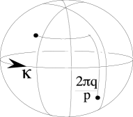
Figure 2: Standard spine of $L(p,q)$ and core $\kappa$

Thin presentation of knots in closed $3$-manifolds

Now, we define the thin presentation of a knot in $M$ with respect to a spine $\Sigma$. We note $M=\hbox{$B_{/_{\sim_{\partial}}}$}$ according to the spine $\Sigma=\partial B_{/\sim_{\partial}}$.

Let $\infty$ be an interior point of the $3$-ball $B$. Then $M-(\Sigma\cup\{\infty\})\cong S^{2}\times\mathbb{R}_{>0}$. So, we have an associated height function $h:M-(\Sigma\cup\{\infty\})\rightarrow\mathbb{R}_{>0}$ which is the projection on the second factor. We extend $h$ to $\Sigma$ by setting $h|_{\Sigma}=0\in\mathbb{R}_{\geq 0}$, so $h(M-\{\infty\})=\mathbb{R}_{\geq 0}$. The level $2$-spheres are the spheres $\hbox{$\widehat{Q}$}_{t}=S^{2}\times\{t\},\ t\in]0,+\infty[$.

Let $K$ be a knot in $M$. By an isotopy of $K$, we may assume that $K\subset M-\{\infty\}$ is transverse to $\Sigma$ and $h|_{K}$ is a Morse function.

Similarly as for knots in $S^{3}$, between each pair of consecutive critical values of $h|_{K}$, the level $2$-spheres of the foliation have the same geometric intersection number with the knot (Figure 3). Given such a Morse presentation of $K$, let $S_{1},\dots,S_{m}$ be level $2$-spheres, one between each pair of consecutive critical levels. Furthermore, let $S_{0}$ be a level $2$-sphere between $\Sigma$ and the first critical level. So, $\widehat{Q}_{0}=S_{0}=\partial N(\Sigma)$, where $N(\Sigma)$ is a regular neighbourhood of $\Sigma$.

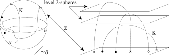
Figure 3: Morse presentation in a $3$-manifold

We then call the number $\displaystyle\#(K)=\sum_{i=0}^{m}|S_{i}\cap K|$ the complexity of the Morse presentation. A thin presentation of $K$ is a Morse presentation of minimal complexity; that is, precisely a presentation of the knot obtained by further isotopies of $K$ in $M-\Sigma\cong M-IntN(\Sigma)$ on a given Morse presentation to minimize the complexity. In a thin presentation, one cannot decrease $\displaystyle\#(K)-s_{0}=\sum_{i=1}^{m}|S_{i}\cap K|$.

We denote $M_{K}=M-$int$N(K)$, the exterior of the knot $K$. A properly embedded surface in $M_{K}$, isotopic to $Q_{t}=\hbox{$\widehat{Q}$}_{t}\cap M_{K}$ is called a level surface of the presentation. Remark that $Q_{0}=\hbox{$\widehat{Q}$}_{0}\cap M_{K}=S_{0}\cap M_{K}$ is (still) in a regular neighbourhood of $\Sigma\cap M_{K}$.

Note first that $\Sigma$ is not necessary a minimal spine; i.e. a spine with a minimal intersection number with the knot among all spines of the $3$-manifold. Thin presentations of $K$ are defined with an arbitrary choosen spine $\Sigma$.

And finally note that if, for a presentation, $K$ intersects the singular set of $\Sigma$ then $h|_{K}$ is not a Morse function (because of the openess property of being a Morse function).

We will see, in Section 4 that in certain conditions we can minimize the intersection between $K$ and a standard spine $\Sigma$ of a lens space, by allowing intersection with $\kappa$, the singular set of $\Sigma$.

Associated intersection graphs

Let $k$ be a knot in $S^{3}$ and $M=X_{k}(r)$ the $3$-manifold obtained by $r$-Dehn surgery on $k$. Recall that $k_{r}$ denotes the core of the surgery and $X_{k}=S^{3}-$int$N(k)\cong M-$int$N(k_{r})=M_{k_{r}}$.

Let us consider a thin presentation of $k$ in $S^{3}$ and a thin presentation of $k_{r}$ in $M$, associated to any spine.

Let $\widehat{P}$ and $\widehat{Q}$ denote level $2$-spheres in the foliations of $S^{3}$ and $M$, respectively and $P=\hbox{$\widehat{P}$}\cap X_{k}$ and $Q=\hbox{$\widehat{Q}$}\cap X_{k}$ be the corresponding level surfaces. Then $P$ and $Q$ are planar surfaces, properly embedded in $X_{k}$. The torus boundary $T_{k}=\partial X_{k}$ contains the slopes $r$ and $\infty$, and each component of $\partial P$ (resp. $\partial Q$) represents $\infty$ (resp. $r$). Moreover, up to isotopies, $P$ and $Q$ are transverse, and each component of $\partial P$ intersects each component of $\partial Q$ exactly $\Delta$ times, where $\Delta$ is $\Delta(\infty,r)$, the geometric intersection number between $r$ and $\infty$ on $T_{k}$.

Let us recall the construction of intersection graphs coming from a pair of planar surfaces properly embedded in $X_{k}$; this is described in details in [18, 22].

Let $(G,H)$ denote the pair of graphs associated to $(\hbox{$\widehat{P}$},\hbox{$\widehat{Q}$})$. Capping off the boundary components of $P$ (resp. $Q$) with meridional disks of $N(k)$ (resp. of $N(k_{r})$), we regard these disks as defining the “fat” vertices of the graph $G$ (resp. $H$) in $\widehat{P}$ (resp. in $\widehat{Q}$). The edges of $G$ (resp. $H$) are the arc-components of $P\cap Q$ in $P$ (resp. in $Q$).

The endpoints of edges in $G$ and $H$ can be labelled in the following way. We first number the components of $\partial P$ and $\partial Q$ in the order they appear (successively) on $T_{k}$. Let number the components of $\partial P$: $V_{1},V_{2},\dots,V_{p}$; and those of $\partial Q$: $W_{1},W_{2},\dots,W_{q}$. We then label the endpoints of an arc of $P\cap Q$ in $P$ (resp. in $Q$) with the numbers of the corresponding components of $\partial Q$ (resp. of $\partial P$) that intersect $P$ (resp. in $Q$) to create these endpoints. Thus, around each component of $\partial P$ (resp. $\partial Q$), we see the labels $\{1,2,\dots,q\}$ (resp. $\{1,2,\dots,p\}$) appearing in this order (either clockwise or anticlockwise). So these labels of the arcs of $P\cap Q$ allows us to label the endpoints of edges in $G$ and $H$ whether the arcs are viewed in $P$ or $Q$, respectively.

A vertex is positive if the labels appear clockwise around it; otherwise, we say it is negative. And two vertices are parallel if they have the same sign, i.e. they are both positive or both negative; otherwise they are antiparallel.

In this framework, we say that the pair of graphs $(G,H)$ is of type $(\hbox{$\widehat{P}$},\hbox{$\widehat{Q}$})$.

If $P$ and $Q$ are orientable surfaces, we have the so called parity rule [8]: an edge $e$ in $G$ joins two parallel vertices if and only if $e$ joins two antiparallel vertices in H.

Let $G^{0}$ and $G^{1}$ denote the set of vertices and edges of $G$, respectively. A face of $G$ is the closure of a connected component of $\hbox{$\widehat{P}$}-(G^{1}\cup G^{0})$. Similarly, we denote $H^{0}$ and $H^{1}$, the set of vertices and edges of $H$, respectively, and we have the same definitions for the faces of $H$.

Let $\Gamma$ be $G$ or $H$. A cycle in $\Gamma$ is a subgraph of $\Gamma$ homeomorphic to a circle when vertices are considered as points; the length of the cycle is the number of its edges. Note that if a cycle in $\Gamma$ bounds a face of $\Gamma$, then this face is necessarily a disk; we will then say that it is a disk-face. Two edges are said to be parallel in $\Gamma$ if they form a cycle of length two which bounds a disk-face of $\Gamma$.

Two particular cycles play a key-role in the following. A trivial loop is a cycle of length one which bounds a disk-face; see Figure 4(b). A Scharlemann cycle is a cycle which bounds a disk-face, such that for an orientation of the cycle, all the edges have the same label at their sink, $x$ say, and also at their source, $y$ say. Consequently $y=x\pm 1\ (mod\ \zeta)$ (where $\zeta$ is $p$ or $q$ according to $\Gamma$ is $H$ or $G$ respectively). These labels $\{x,y\}$ are called the labels of the Scharlemann cycle; see Figure 5(b). And we then say that this is a $\{x,y\}$-Scharlemann cycle.

Links between foliations and intersection graphs

For a $M$-foliation, a level $2$-sphere $\widehat{Q}$ separates $M$ in two connected components; one of these contains the spine $\Sigma$ and we say it below $\widehat{Q}$ (or below the level of $\widehat{Q}$), the other component setting to be above $\widehat{Q}$. With these definitions, we have also implicitly set what do we mean by a presentation beginning by a local maximum (resp. minimum).

We set above a level $2$-sphere $\widehat{P}$ in a $S^{3}$-foliation, the component of $S^{3}-$$\widehat{P}$ containing $+\infty$; if containing $-\infty$, it is below $\widehat{P}$.

In this paragraph, we keep the hypothesis and notations of the previous. Let $\{X,Y\}=\{P,Q\}$.

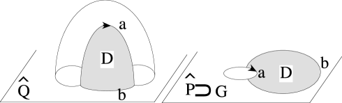
(a)High disk in $P$       (b)Trivial loop in $G$

Figure 4:

Then, $X$ is said to be high (resp. low) with respect to $Y$ if there exists a disk $D\subset Y$ below (resp. above) $X$ with $\partial D=a\cup b$ such that $a=D\cap\partial X_{k}$ and $b=D\cap X$ are simple arcs (Figure 4(a)).

The existence of such a (high or low) disk in $P$ (resp. in $Q$) is equivalent to the existence of a trivial loop in the graph $G$ (resp. $H$); see Figure 4(b).

Now, we define a characteristic corresponding to the existence of a Scharlemann cycle. We say that a disk $D\subset Y$ is carrying if the two following conditions are satisfied, for an orientation of $\partial D$ (Figure 5(a)).

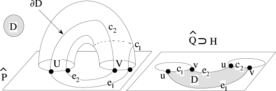
(a)Carrying disk in $Q$    (b)Scharlemann cycle in $H$

Figure 5:

$D\cap X=\partial D\cap X$ is the disjoint union of $n$ simple arcs, $e_{1},\dots,e_{n}$ which join the same components $U$ and $V$ of $\partial X$ and are all oriented from $V$ to $U$;

$\partial D\cap\partial X_{k}$ is the disjoint union of $n$ simple arcs, $c_{1},\dots,c_{n}$, all oriented from $U$ to $V$ in $\partial X_{k}$;

We say that $X$ is carrier with respect to $Y$ if there exists a carrying disk $D\subset Y$.

The existence of such a carrying disk in $Q$ (resp. in $P$) is equivalent to the existence of a Scharlemann cycle in the graph $H$ (resp. $G$); see Figure 5(b). Actually, the vertices $U$ and $V$ in the above definition are consecutive ones (in terms of labels) in the graph lying on $X$.

3 The generic case

Let $M$ be a closed $3$-manifold that does not contain a lens space as a connected summand; here the connected sum can be trivial, that is we exclude the cases where $M$ would be a lens space (or $S^{3}$ or $S^{1}\times S^{2}$). Let $K$ be a knot in $M$ yielding $S^{3}$ by $\gamma$-Dehn surgery; note $K_{\gamma}$ the core of the surgery.

Proof of Theorem 1.1 Suppose for a contradiction that a thin presentation of $K$ in $M$ has a local minimum.

A middle slab in a thin presentation of a knot is a family of level $2$-spheres, between consecutive local minimum and local maximum (of the thin presentation). Let $K_{\gamma}$ be in a thin presentation in $S^{3}$.

Consequently, the above thin presentations gave both middle slabs, denoted $\mathcal{M}$ and $\mathcal{M}^{\prime}$ respectively. Therefore, by [22, Proposition 1], there is a pair of level $2$-spheres $(\hbox{$\widehat{P}$},\hbox{$\widehat{Q}$})$ in $(\mathcal{M},\mathcal{M}^{\prime})$ such that $P$ is neither low nor high with respect to $Q$, and vice-versa. Equivalently, the pair of graphs $(G,H)$ of type $(\hbox{$\widehat{P}$},\hbox{$\widehat{Q}$})$, does not contain a trivial loop. Note that $\widehat{P}$ and $\widehat{Q}$ are separating $2$-spheres because they are level spheres. Thus, we can apply the following combinatorial result, due to Gordon and Luecke.

Theorem 3.1[22, Proposition 2.0.1] Let $(G,H)$ be a pair of intersection graphs of type $(S^{2},S^{2})$ without trivial loop. If $H$ does not represent all types then $G$ contains a Scharlemann cycle, and vice-versa.

Moreover, if $H$ represents all types then $S^{3}$ contains a $3$-sub-manifold with non-trivial torsion ([22, Section 3] or [34]) which is impossible. Consequently, $G$ contains a Scharlemann cycle, and so $M$ contains a lens space as a connected summand by [8, Lemma 2.5.2.b], which is the required contradiction proving Theorem 1.1.

Intersection with all spines

To conclude this section, we prove the following.

Lemma 3.2 $K$ intersects all the spines of $M$.

Proof.

Let $M_{K}=M-$Int$N(K)$ and $M_{K}(\gamma)$ be the $3$-manifold obtained by $\gamma$-Dehn surgery on $K$. Assume $M_{K}(\gamma)=S^{3}$ and note that $\gamma$ is not the meridional slope of $K$, otherwise $M_{K}(\gamma)=M=S^{3}$.

We consider $M$ as $B_{/_{\sim_{\partial}}}$, and denote $\Sigma=S_{/\sim_{\partial}}$, the corresponding spine. Let $s$ be the geometric intersection number between $K$ and $\Sigma$. If $s=0$ then $K$ lies in Int$B$, and $M_{K}(\gamma)=M\#B_{K}(\gamma)$. Consequently, $M_{K}(\gamma)$ is $M$ or a reducible $3$-manifold, in contradiction with $S^{3}$. ∎

In all the following, we consider the case where $M$ is a lens space.

4 Lens space case

Let $K$ be a knot in a lens space $L$, and $\Sigma$ be a standard spine in $L$. Let us suppose that $K$ is in a thin presentation, with respect to $\Sigma$. Let $\kappa$ be the core of $\Sigma$, that is the $1$-dimensional singular sub-complex of $\Sigma$ (Figure 2).

Let $\mu$ be the level of a local maximum. Denote $\alpha_{\mu}$ the arc on $K$ realizing this local maximum; that is the arc on $K$ that starts on the spine $\Sigma$, goes up straight through the level spheres, passes tangently by the level $\mu$ and goes down straight through the level spheres, back to $\Sigma$ (Figure 6). Let $D_{\mu}$ be a disk properly embedded in $L_{K}-\Sigma$ where $\partial D_{\mu}=\alpha\cup\beta$ is such that:

$\alpha=\partial L_{K}\cap D_{\mu}=\partial L_{K}\cap\partial D_{\mu}$ is an arc parallel to $\alpha_{\mu}$,

$\beta=\Sigma\cap D_{\mu}=\Sigma\cap\partial D_{\mu}$ is an arc.

Remark that $\beta$ must intersect the core $\kappa$ of $\Sigma$ in a several finite number of points.

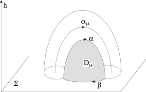
Figure 6: Inessential local maximum

If there is such a disk then the corresponding local maximum at level $\mu$ is said to be inessential. This means that the local maximum $\alpha_{\mu}$ can be isotoped, to $\beta$ in $\Sigma$. For such an inessential local maximum $\mu_{1}$, let us do the isotopy of $\alpha_{\mu_{1}}$ to $\Sigma$. Then if there is another inessential local maximum $\mu_{2}$, let us do the same. And so on, until there is no more disk $D_{\mu}$ as we described above. We then obtain a particular presentation of the knot $K$ that we call essential thin presentation.

If an essential thin presentation of $K$ begins by a local maximum then this local maximum is not inessential in the thin presentation; i.e. it cannot be isotoped onto $\Sigma$. We call it essential local maximum.

Let us note that an inessential local maximum is necessarily below the first local minimum (if there is) in the thin presentation of $K$. And also note that any local maximum above a local minimum must be essential because of the thinness of the presentation of $K$.

Now, suppose that $K$ is a knot in a lens space $L$ yielding $S^{3}$ by Dehn surgery. The remaining of this section is devoted to the proof of the following result.

Theorem 4.1 If an essential thin presentation of $K$, with respect to the standard spine $\Sigma$, begins by a local maximum then $s=1$.

As usual, let $K_{\gamma}$ denote the core of the surgery in $S^{3}$ and remark that $L_{K}=L-$Int$N(K)\cong S^{3}-intN(K_{\gamma})=X_{K_{\gamma}}$. So, let us consider a $S^{3}$-foliation in which $K_{\gamma}$ is in thin presentation and the $L$-foliation associated to an essential thin presentation of $K$ beginning by a local maximum, by hypothesis. Let $\mu^{\prime}$ be the first local maximum level of this essential thin presentation of $K$.

Our goal is now to find two level surfaces $P=\hbox{$\widehat{P}$}\cap L_{K}$, and $Q=\hbox{$\widehat{Q}$}\cap L_{K}$ in the $S^{3}$-foliation and the $L$-foliation respectively, neither high, nor low, nor carrier, one with respect to the other, and vice-versa. Such a result is then in contradiction with Theorem 3.1.

To find this pair of transverse planar surfaces, we use the Cerf Theory [7, Chapter 2] in a similar way as [22].

One-parameter families of $2$-spheres

Recall that a middle slab in a thin presentation of a knot is a family of level $2$-spheres, between consecutive local minimum and local maximum. We then consider:

a middle slab $\{\hbox{$\widehat{P}$}_{\lambda}\}_{\lambda\in I}$ in the $S^{3}$-foliation and

a family of level $2$-spheres $\{\hbox{$\widehat{Q}$}_{\mu}\}_{\mu\in J}$ in the $L$-foliation between $\Sigma$ and the first local maximum.

We may suppose that $I=J=[0,1]$ and for convenience, we fix the index notations $\lambda\in[0,1]$ for $S^{3}$ and $\mu\in[0,1]$ for $L$.

We denote a level $2$-sphere of a foliation $\cal H$, $\cal L$ or $\cal C$ according to its characteristic is $\cal H$igh, $\cal L$ow or $\cal C$arrier and $\cal N$ if it is $\cal N$one of these.

Lemma 4.2

$Q_{\mu}$ cannot be $\cal L$ for all $\mu<\mu^{\prime}$.

There exists $\mu_{0}<\mu^{\prime}$ such that $Q_{\mu}$ is $\cal C$ for all $\mu<\mu_{0}$.

Proof.

(i)This follows immediatly from the fact that the local maxima are essential in the thin presentation.

(ii)By the previous point, there exists $\mu_{0}<\mu^{\prime}$ such that $Q_{\mu}$ is not $\cal L$ with respect to $P_{\lambda}$, for all $\mu<\mu_{0}$ and all $\lambda\in[0,1]$. Then $Q_{\mu}$ is neither $\mathcal{L}$ nor $\mathcal{H}$, for all $\mu<\mu_{0}$. Therefore, by [15, Lemma 4.4] there exists a level surface $P_{\lambda}$ which is neither $\mathcal{L}$ nor $\mathcal{H}$ with respect to $Q_{\mu}$. The pair of surfaces $(P_{\lambda},Q_{\mu})$ gives then rise to a pair of intersection graphs $(G,H)$ without trivial loop. Since $S^{3}$ does not contain a $3$-sub-manifold with non trivial torsion, $H$ does not represent all types. Therefore $G$ contains a Scharlemann cycle, by Theorem 3.1, which implies that $Q_{\mu}$ is $\mathcal{C}$, for all $\mu<\mu_{0}$. ∎

Lemma 4.3(Extremal conditions) Without loss of generality, we may suppose that:

$P_{\lambda=0}$ is $\cal H$ and $P_{\lambda=1}$ is $\cal L$; and

$Q_{\mu=0}$ is $\cal C$ and $Q_{\mu=1}$ is $\cal L$.

Proof.

By the previous lemma, the level surfaces $Q_{\mu}$ in a thin neighbourhood of $\Sigma$ must be $\cal C$ so is $Q_{\mu=0}$. Modulo isotopy, we can say that the level surfaces $Q_{\mu}$ in a neighbourhood of $Q_{\mu^{\prime}}$ are $\cal L$ so is $Q_{\mu=1}$. In the same way of isotopies, we have the conditions (i). ∎

Lemma 4.4

If $K_{\gamma}$ is a non-trivial knot then for all $\lambda$, there exists $\mathcal{X}_{\lambda}\in\{\mathcal{H},\mathcal{L}\}$ such that, for all $\mu$, $P_{\lambda}$ is either $\mathcal{N}$ or $\mathcal{X}_{\lambda}$ with respect to $Q_{\mu}$.

If $s\not=1$ then for all $\mu$, there exists $\mathcal{X}_{\mu}\in\{\mathcal{L},\mathcal{C}\}$ such that, for all $\lambda$, $Q_{\mu}$ is either $\mathcal{N}$ or $\mathcal{X}_{\mu}$ with respect to $P_{\lambda}$.

Proof.

(i)If there exists $(\lambda,\mu)$ such that $P_{\lambda}$ is $\mathcal{C}$ with respect to $Q_{\mu}$ then the graph $G\subset\hbox{$\widehat{Q}$}_{\mu}$ of the associated pair of intersection graphs $(G,H)$, contains a Scharlemann cycle, which implies that $S^{3}$ contains a (non-trivial) lens space as a connected summand [8, Lemma 2.5.2.b]. Therefore for all $(\lambda,\mu),\ P_{\lambda}$ is never $\mathcal{C}$ with respect to $Q_{\mu}$.

Now, assume that there exist $\lambda,\mu_{1}$ and $\mu_{2}$ such that $P_{\lambda}$ is $\cal H$ with respect to $Q_{\mu_{1}}$ and $\cal L$ with respect to $Q_{\mu_{2}}$. Then, by [22, Lemma 1.1] if $K_{\gamma}$ is not trivial, the low and high disks give an isotopy on $K_{\gamma}$ that leads to a minimization of the complexity, which is a contradiction.

(ii)Since $\mu<\mu^{\prime},\ Q_{\mu}$ cannot be $\cal H$. So, assume there exist $\lambda_{1},\lambda_{2}$ and $\mu$ such that $Q_{\mu}$ is $\cal C$ with respect to $P_{\lambda_{1}}$ and $\cal L$ with respect to $P_{\lambda_{2}}$. Let $b$ denote the arc component of the intersection of the high disk (in $P_{\lambda_{2}}$) with $Q_{\mu}$ (see Figure 4(a)) and $\{e_{i}\}_{1\leq i\leq n}$ the arc components of the intersection between the carrying disk (in $P_{\lambda_{1}}$) and $Q_{\mu}$ (see Figure 5(a)). Since there is no local minimum of level lower than $\mu^{\prime}$, the arc $b$ can be isotoped in $X$, to $\Sigma$. The isotopy define a disk $D_{\mu^{\prime}}$ such that $\mu^{\prime}$ corresponds to an inessential local maximum because $b$ does not intersect the carrying disk and so $D_{\mu^{\prime}}$ cannot be a singular disk. But this is a contradiction. ∎

Graph of singularities

From now on, we suppose that $K_{\gamma}$ is not trivial, and $s\not=1$. For convenience, we say that a level surface $P_{\lambda}$ or $Q_{\mu}$ is at most $\cal H,\cal L$ or $\cal C$, in reference to the previous lemma. Note that $P_{\lambda}$ is never $\mathcal{C}$ and $Q_{\mu}$ is never $\mathcal{H}$.

Let $\Gamma$ be the Cerf graph of singularities, representing the singularities which appear in the intersection of two one-parameter families of surfaces (Figure 7).

A point in $\Gamma$ is a couple of parameters $(\lambda,\mu)\in[0,1]^{2}$ for which the corresponding surfaces $P_{\lambda}$ and $Q_{\mu}$ are tangents; a point in the exterior of the graph $\Gamma^{c}=[0,1]^{2}-\Gamma$, corresponds to transverse surfaces.

Figure 7: Graph of singularities

Only two types of singular points can appear in $\Gamma$:

Index $1$ point

which corresponds to interchange of two tangency points. For example, the surface $P_{\lambda=i-\varepsilon}$ in Figure 7, has two tangency points on two different levels (for two surfaces $Q_{\mu_{1}}$ and $Q_{\mu_{2}}$). Now, decreasing $\varepsilon$ through $0$, these two points pass through the same level as tangency points between $P_{\lambda=i}$ and some surface $Q_{\mu}$.

Index $2$ point

which corresponds to birth/death of two tangency points. For example, the surface $P_{\lambda=j-\varepsilon}$ in Figure 7, has two tangency points on two different levels which degenerate in a single tangency point for $\varepsilon$ decreasing to $0$ and disappears for $\lambda>j$.

All such singular points of $\Gamma$ can be supposed, without loss of generality, with distinct abscissa $\lambda$, and also with distinct ordinates $\mu$.

Moreover, the slope of such a graph can be supposed neither vertical nor horizontal. These conditions can be realized by transversality arguments due to Cerf [7, Chapter 2]. Furthermore, by isotopies on $\{P_{\lambda}\}_{\lambda\in[0,1]}$, the extremal conditions (Lemma 4.3) continue to hold. Note that all conditions we work with, are open ones.

Lemma 4.5 For all $(\lambda,\mu)$ in a connected component of $\Gamma^{c}$, all the $P_{\lambda}$ have the same characteristic in $\{\mathcal{H},\mathcal{L},\mathcal{N}\}$ with respect to $Q_{\mu}$; and similarly, all the $Q_{\mu}$ have the same characteristic in $\{\mathcal{C},\mathcal{L},\mathcal{N}\}$ with respect to $P_{\lambda}$.

Proof.

Because $P_{\lambda}\cap Q_{\mu}$ cannot change its isotopy class, except as passing through a point of the graph $\Gamma$. ∎

So, we can associate to each component of $\Gamma^{c}$ two characteristics from the set $\{\cal H,\cal L,\cal C,\cal N\}$: one with respect to $\lambda$ and the other, with respect to $\mu$.

From Lemmas 4.4 and 4.5, we then obtain:

Corollary 4.6

Let $\lambda_{1}\in[0,1]$ and $\Lambda_{1}$ the set of the connected components of $\Gamma^{c}$ intersecting the vertical line $\lambda=\lambda_{1}$. Then there exists $\mathcal{X}\in\{\mathcal{H},\mathcal{L}\}$ such that, for all $(\lambda,\mu)$ in $\Lambda_{1}$, $P_{\lambda}$ have the characteristic $\mathcal{X}$ or $\mathcal{N}$ with respect to $Q_{\mu}$.

Let $\mu_{1}\in[0,1]$, and $\Lambda_{1}$ the set of the connected components of $\Gamma^{c}$ intersecting the horizontal line $\mu=\mu_{1}$. Then there exists $\mathcal{X}\in\{\mathcal{L},\mathcal{C}\}$ such that, for all $(\lambda,\mu)$ in $\Lambda_{1}$, $Q_{\mu}$ have the characteristic $\mathcal{X}$ or $\mathcal{N}$ with respect to $P_{\lambda}$.

Lemma 4.7

$\forall\lambda\in[0,1]\ \ \exists\mu\in[0,1]\ |\ (\lambda,\mu)\in\Gamma^{c}$ and $Q_{\mu}$ is $\cal N$ with respect to $P_{\lambda}$.

$\forall\mu\in[0,1]\ \ \exists\lambda\in[0,1]\ |\ (\lambda,\mu)\in\Gamma^{c}$ and $P_{\lambda}$ is $\cal N$ with respect to $Q_{\mu}$.

Proof.

(i)Assume for a contradiction that there exists $P_{\lambda_{1}}$, such that $Q_{\mu}$ is either $\cal L$ or $\cal C$ with respect to $P_{\lambda_{1}}$, for all $\mu\in[0,1]$ with $(\lambda_{1},\mu)\in\Gamma^{c}$. By Lemma 4.4, $Q_{\mu}$ cannot be $\cal L$ and $\cal C$. Therefore, there exists a saddle tangency level, $\mu_{1}$, in $P_{\lambda_{1}}$, which is above the Carrier spheres $Q_{\mu<\mu_{1}}$ and below the Low spheres $Q_{\mu>\mu_{1}}$.

Let $\varepsilon>0$ and $\displaystyle\bigcup_{i=\lambda_{1}-\varepsilon}^{i=\lambda_{1}+\varepsilon}P_{i}$ a regular neighbourhood of $P_{\lambda_{1}}$. Since $\mu_{1}$ corresponds to a saddle point, $Q_{\mu_{1}}$ is $\cal L$ and $\cal C$ with respect to $P_{\lambda_{1}-\varepsilon}$ and $P_{\lambda_{1}+\varepsilon}$, respectively; in contradiction with Lemma 4.4.

(ii)We apply the same argument, changing the Carrier characteristic to the High one. ∎

Claim 4.8 Without loss of generality, we may suppose that there is no pair $(\lambda,\mu)\in\Gamma^{c}$ such that $P_{\lambda}$ and $Q_{\mu}$ are both $\mathcal{N}$ one with respect to the other.

Proof.

Otherwise the associated pair of intersection graphs is in contradiction with the Theorem 3.1. ∎

Therefore, in a same connected component of $\Gamma^{c}$, we cannot have both characteristics of $P_{\lambda}$ and $Q_{\mu}$ to be $\cal N$.

Let $t=\sup\{\mu\in[0,1]\mid Q_{\mu}\ {\rm{is}}\ \cal C\}$; so $0<t<1$, by Lemma 4.3. Since the slopes of $\Gamma$ are non-horizontal, the corresponding point $(s,t)\in\Gamma$ is a singular point.

If $(s,t)$ is an index $2$ point then there are exactly two connected components of $\Gamma^{c}$ in a neighbourhood of $(s,t)$. Therefore, from Corollary 4.6(ii), the level surfaces $Q_{\mu}$ have characteristic $\cal C$ in one of them and $\cal N$ in the other, with respect to all the corresponding $P_{\lambda}$’s.

Furthermore, $Q_{\mu=t+\varepsilon}$ is $\cal N$ with respect to $P_{\lambda}$ for all $\lambda\in[0,1]$; otherwise, as $t=\sup\{\mu\in[0,1]\mid Q_{\mu}\ {\rm{is}}\ \cal C\}$ we could find $\lambda_{1},\lambda_{2}$ such that $Q_{\mu=t-\varepsilon}$ is $\mathcal{C}$ for $P_{\lambda_{1}}$ and $Q_{\mu=t-\varepsilon}$ is $\mathcal{L}$ for $P_{\lambda_{2}}$, in contradiction with Lemma 4.4(i). By Lemma 4.7, we can find $P_{\lambda}$ and $Q_{\mu}$, each being $\cal N$ with respect to the other; which is impossible by the previous claim.

Consequently, we may assume that $(s,t)$ is an index $1$ point.

Figure 8: Configuration of $(s,t)$ in $\Gamma$

Lemma 4.9 The graph $\Gamma$, in a neighbourhood of the point $(s,t)$ is described in Figure 8 with the following properties:

$(\lambda,\mu)\in R_{1}\Rightarrow P_{\lambda}$ is $\cal H$ with respect to $Q_{\mu}$ and $Q_{\mu}$ is $\cal N$ with respect to $P_{\lambda}$.

$(\lambda,\mu)\in R_{2}\Rightarrow P_{\lambda}$ is $\cal N$ with respect to $Q_{\mu}$ and $Q_{\mu}$ is $\cal C$ with respect to $P_{\lambda}$.

$(\lambda,\mu)\in R_{3}\Rightarrow P_{\lambda}$ is $\cal L$ with respect to $Q_{\mu}$ and $Q_{\mu}$ is $\cal N$ with respect to $P_{\lambda}$.

$(\lambda,\mu)\in R_{4}\Rightarrow P_{\lambda}$ is $\cal N$ with respect to $Q_{\mu}$ and $Q_{\mu}$ is $\cal L$ with respect to $P_{\lambda}$.

Proof.

The definition of $t$ implies $Q_{\mu}$ is $\mathcal{C}$ with respect to $P_{\lambda}$, for $(\lambda,\mu)\in R_{2}$ and $Q_{\mu}$ is not $\mathcal{C}$ with respect to $P_{\lambda}$, for $(\lambda,\mu)\in R_{4}$; so is $\mathcal{L}$ or $\mathcal{N}$ in $R_{4}$.

As singular points of $\Gamma$ are on different ordinates, $(s,t)$ is the only singular point of $\Gamma$ in $N(\mu=t)=[0,1]\times[t-\varepsilon,t+\varepsilon]$ for small enough $\varepsilon$. So, as $Q_{\mu}$ is $\mathcal{C}$ in $R_{2}$, Corollary 4.6(ii) implies:

$Q_{\mu}$ is $\mathcal{N}$ with respect to $P_{\lambda}$ for all $(\lambda,\mu)\in N(\mu=t)\backslash(R_{2}\cup R_{4})$  $(*)$

Furthermore, if we suppose $Q_{\mu}$ is $\mathcal{N}$ in $R_{4}$ then, by Lemma 4.7(ii), we deduce a contradiction to Claim 4.8. Then $Q_{\mu}$ is $\mathcal{L}$ in $R_{4}$ and $\mathcal{N}$ in $R_{1}\cup R_{3}$.

So, Claim 4.8 again implies $P_{\lambda}$ is not $\mathcal{N}$ in $R_{1}\cup R_{3}$ and $(*)$ implies $P_{\lambda}$ is not $\mathcal{N}$ in $N(\mu=t)\backslash(R_{2}\cup R_{4})$. And from Lemma 4.3 (Extremal conditions), we conclude $P_{\lambda}$ is $\mathcal{H}$ and $\mathcal{L}$ in $R_{1}$ and $R_{3}$, respectively. Finally, Corollary 4.6(i) implies $P_{\lambda}$ is $\mathcal{N}$ in $R_{2}\cup R_{4}$. ∎

For convenience, we note $\lambda=s\pm\varepsilon$, abscissa of points in $\Gamma$, in a regular neighbourhood of $s$. And similarly for ordinates $\mu=t\pm\varepsilon$, in a neighbourhood of $\mu=t$. Note that (see Figure 8) there exist $\varepsilon^{\prime}>0$ and $C_{\lambda}$, $C^{\prime}_{\lambda}$ with $t-\varepsilon^{\prime}<C_{\lambda}<t<C^{\prime}_{\lambda}<t+\varepsilon^{\prime}$ such that:

$P_{\lambda=s-\varepsilon}$ and $Q_{\mu=C_{\lambda}}$ are tangents in a point $x_{\lambda}$.

$P_{\lambda=s-\varepsilon}$ and $Q_{\mu=C^{\prime}_{\lambda}}$ are tangents in a point $x^{\prime}_{\lambda}$.

$x_{\lambda}$ and $x^{\prime}_{\lambda}$ are in the boundary of $R_{1}$ (on different lines of $\Gamma$).

Therefore, the point $(s,t)\in\Gamma$ is an index $1$ point, which corresponds to a pair of saddle-points $x=x_{\lambda=s}$ and $x^{\prime}=x^{\prime}_{\lambda=s}$ which are the two tangency points between the surfaces $P_{\lambda=s}$ and $Q_{\mu=t}$. For convenience, the reader should refer, say [22, p.381].

Let $D^{-}$ and $D^{+}$ be the limits in $Q_{\mu=t}$ when $\lambda$ goes to $s$, of the low and high disks for $P_{\lambda}$ coming from $R_{1}$ and $R_{3}$, respectively. Then the boundary of $D^{-}$ (resp. $D^{+}$) contains $x$ and $x^{\prime}$.

Indeed, if for example $x\notin\partial D^{-}$ then the low disk for $(\lambda,\mu)\in R_{1}$ does not disappear when $(\lambda,\mu)$ goes through the line defined by $\{\mu=C_{\lambda}\}$ (Figure 8). Therefore $P_{\lambda}$ is still high with respect to $Q_{\mu}$ for $(\lambda,\mu)\in R_{2}$ and this is in contradiction with Lemma 4.7.

If $x^{\prime}\notin\partial D^{-}$ then we pass the low disk of $R_{1}$ through the line defined by $\{\mu=C^{\prime}_{\lambda}\}$ (Figure 8), surviving so in $R_{4}$ in contradiction with Lemma 4.7.

For the case $x\notin\partial D^{+}$, one can pass the high disk from $R_{3}$ to $R_{4}$ and for the case $x^{\prime}\notin\partial D^{+}$, from $R_{3}$ to $R_{2}$; arriving also at a contradiction.

Trying to put the limit-disks $D^{-}$ and $D^{+}$ in $Q_{\mu=t}$, we deduce the configuration on $Q_{\mu=t}$ of Figure 9(a); otherwise $P_{\lambda=s}$ has only two boundary components, and hence $K_{\gamma}$ is trivial in $S^{3}$. Let $V_{1}$ and $V_{2}$ denote the boundary components of $Q_{\mu=t}$ that $D^{+}$ and $D^{-}$, respectively meet (Figure 9(a)); see [22, pp. 383-384], for convenience.

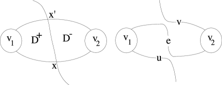
(a)$D^{\pm}$ in $Q_{\mu=t}$     (b)$b_{\varepsilon}$ in $Q_{\mu=t+\varepsilon}\cap P_{\lambda=s}$

Figure 9:

Now we look at the characteristics $\mathcal{C}$ and $\mathcal{L}$ of $Q_{\mu}$, with respect to $P_{\lambda}$, that is for $(\lambda,\mu)$ in $R_{2}$ and $R_{4}$, respectively. The characteristic $\cal L$ in $R_{4}$ gives rise to a high disk $D_{\varepsilon}$ ($\subset P_{\lambda=s}$) whose boundary contains an arc $b_{\varepsilon}$ in $Q_{\mu=t+\varepsilon}$, i.e. $b_{\varepsilon}=\partial D_{\varepsilon}\cap Q_{\mu=t+\varepsilon}=D_{\varepsilon}\cap Q_{\mu=t+\varepsilon}$. Let $b^{+}$ be its limit for $\varepsilon$ decreasing to $0$. Then $b^{+}$ is a simple arc properly embedded in $Q_{\mu=t}$, which contains $x$ and $x^{\prime}$ for the same reason as above with $\partial D^{-}$ (and $\partial D^{+}$).

Furthermore, $x$ and $x^{\prime}$ are saddle-points, so we describe in Figure 9(b) the local intersection in $Q_{\mu=t+\varepsilon}$ with $P_{\lambda=s}$.

Let $e$ be the arc in $Q_{\mu=t+\varepsilon}$, joining $V_{1}$ and $V_{2}$, which corresponds to the arc in $Q_{\mu=t}$ joining $V_{1}$ and $V_{2}$, and passing through $x^{\prime}$ and $x$ (Figure 9(a)). Let $u$ and $v$ be the remaining open arcs. Then either $b_{\varepsilon}$ contains $e$ or $u\cup v$. Consequently, $b^{+}$ joins the two components $V_{1}$ and $V_{2}$.

Likewise, the characteristic $\cal C$ in $R_{2}$ gives an union of arcs in $Q_{\mu=t-\varepsilon}$. Their limit $b^{-}$ (union of arcs) must also contain $x$ and $x^{\prime}$. Furthermore, $V_{1}$ and $V_{2}$ are joined by $b^{-}$, as well as for $b^{+}$ above.

Thus the knot $K$ intersects exactly twice the sphere $Q_{\mu=t}$ and once the spine $\Sigma$. So $s=1$, proving Theorem 4.1.

5 Geometric intersection with a lens spine

Let $K$ be a knot in a lens space $L$, which produces $S^{3}$ by $\gamma$-Dehn surgery. Let $\Sigma$ be a standard spine of $L$, and $s$ be the minimal geometric intersection number between $K$ and $\Sigma$. Let $K_{\gamma}$ be the core of the surgery in $S^{3}$.

A $(m,n)$-cable of a knot $k$, is a knot lying on the boundary of a regular neighbourhood of $k$, which goes $m$ times in the meridional direction and $n$ times in the longitudinal. And non-trivial cables of torus knots are known to produce lens spaces by Dehn surgery [2, 20]. Note that cables of the trivial knot (or $0$-bridge braids) in $S^{3}$ are exactly the torus knots.

Lemma 5.1 Assume that $s=1$.

If a thin presentation of $K$, with respect to $\Sigma$, begins by a local maximum then $K$ is a $0$ or $1$-bridge braid in $L$.

If a thin presentation of $K$, with respect to $\Sigma$, begins by a local minimum then $K_{\gamma}$ is a cable in $S^{3}$.

Proof.

(i)The knot $K$ intersects exactly twice the sphere $S=\partial N(\Sigma)$. Let $X$ be the $3$-ball bounded by $S$, and $a=K\cap X$, then $(a,X)$ is a trivial tangle, since $a$ is a “local maximum”. Therefore there is a disk, $D$ say, in $X$ such that $\partial D=a\cup b$, where $b$ is a simple arc in $S$. Then, we can isotope $a$, successively via $D$ and $N(\Sigma)$, to a simple arc $\alpha$ in $\Sigma$, with its endpoints identified, since $s=1$.

Let $\kappa$ be the core of the spine. Then $\alpha$ and $\kappa$ “cobound” a pinched spinal helix of order less than $\hbox{\ssmall order of }\Sigma\over 2$ (Figure 10). In other words, $K$ is isotoped to a simple closed curve in $\Sigma$ which intersects the core $\kappa$ only once. Thus, $K$ is isotoped to $\alpha$ and therefore, is a $0$ or $1$-bridge braid in $L$.

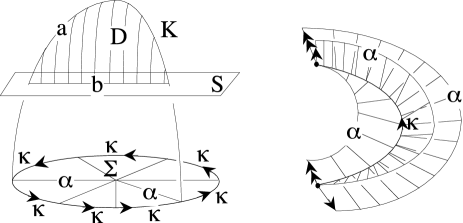
(a)High disk until $\alpha\subset\Sigma$     (b)Pinched spinal helix

Figure 10:

(ii)Let $\widehat{Q}=\partial N(\Sigma)$ be a level $2$-sphere of the thin presentation of $K$, in a neighbourhood of the spine. And denote $Q=\widehat{Q}\cap L_{K}$, the corresponding level surface. Since $|\widehat{Q}\cap K|=2$ and the thin presentation of $K$ begins by a local minimum, we deduce that $Q$ is incompressible and $\partial$-incompressible in $L_{K}$. Fixing a thin presentation of $K_{\gamma}$ in $S^{3}$, $Q$ is a properly embedded planar surface in $X_{K_{\gamma}}$ such that $\partial Q$ is not meridional. Therefore, by [15, Lemma 4.4], one can find a level surface $P$ from the $S^{3}$-foliation, transverse to $Q$ in $L_{K}$ with the property that $P$ (and already $Q$) is neither $\mathcal{L}$ nor $\mathcal{H}$ with respect to $Q$ (resp. $P$).

We can then associate a pair of intersection graphs $(G,H)$ of type $(\hbox{$\widehat{P}$},\hbox{$\widehat{Q}$})$ as in Section 2 such that $G$ and $H$ contain no trivial loop. Now, $H$ has exactly two vertices, therefore the edges in $H$, all join these two with distinct labels at their endpoints. So, $K_{\gamma}$ is a cable knot by [21, Section 5]. ∎

Now Theorem 4.1 and Lemma 5.1(i) prove together Theorem 1.2. Indeed, if we have the hypothesis of Theorem 1.2, so a knot $K$ in an essential thin presentation beginning by a local maximum then Theorem 4.1 applies and Lemma 5.1(i) implies the result.

Proof of Proposition 1.3

Let us suppose, in this paragraph that $K$ is neither a $0$ nor $1$-bridge braid in $L$. And furthermore, let us suppose that $s<3$.

First, if $s=1$ then $K_{\gamma}$ is a cable knot in $S^{3}$ by Lemma 5.1(ii). So, there is a non-meridional essential annulus $A$ in the exterior $X_{K_{\gamma}}=X_{K}$. We also have the level surface $Q$, below the first local minimum, which is an essential annulus in $X_{K}$ transverse to $A$. We obtain a pair of graphs, each with two vertices and without trivial loop. And this contradicts the parity rule.

Now, if $s=2$ and the thin presentation of $K$ is beginning by a local maximum then it is inessential, by Theorem 1.2.

Claim 5.3 If $K$ is standardly spinal then it is a $0$ or $1$-bridge braid.

Proof.

As $s=2$, then $K=\alpha\cup\beta\subset\Sigma$ such that $\alpha\cap\kappa=\beta\cap\kappa=\partial\alpha=\partial\beta$, where $\kappa$ is the core of $\Sigma$. So, $K$ is a $0$ or $1$-bridge braid in $L$. ∎

This claim implies that the thin presentation of $K$ has a local minimum above the first and inessential local maximum. So, by the same argument used in the proof of Lemma 5.1(ii), we deduce that the core of the surgery is a cable knot in $S^{3}$. And using the same reasonning as above for the case $s=1$, we arrive at a contradiction with parity rule.

So, from now on, we may suppose that for $s=2$, we only have the case in which the thin presentation of $K$ begins by a local minimum. Then let $\widehat{Q}$ be the level $2$-sphere in a neighbourhood of the spine $\Sigma$; i.e. such that the corresponding level surface $Q=\partial(N(\Sigma)\cap L_{K})$.

If $Q$ is not incompressible, then there is a compressing disk in $L_{K}$ that cobounds a $3$-ball with a disk $D$ in $\widehat{Q}$; $IntD$ intersects then exactly twice the knot $K$, for its boundary to be essential in $Q$. We isotope $K$, using this $3$-ball, below the first local minimum, reducing so the complexity of the thin presentation of $K$, which is supposed to be impossible. So, $Q$ is incompressible in $L_{K}$. Furthermore, because of the minimal complexity of this presentation beginning by a local minimum, $Q$ is also $\delta$-incompressible.

Then, by [15, Lemma 4.4], we find a level sphere $\widehat{P}$ in a thin presentation of $K_{\gamma}$ in $S^{3}$ such that $P$ is incompressible and $\partial$-incompressible in $X_{K_{\gamma}}=L_{K}$.

So, the pair of graphs $(G,H)$ of type $(\hbox{$\widehat{P}$},\hbox{$\widehat{Q}$})$ does contain no trivial loop. Applying Theorem 3.1, $G$ then contains a Scharlemann cycle $\sigma$ of length $n$, say; let $\{1,2\}$ be the labels of $\sigma$ and $W_{1}$, $W_{2}$ the corresponding vertices in $H$. If $|G^{0}|=p$ and $\Delta=\Delta(\infty,\gamma)$, then there are $\Delta p$ endpoints of edges around each vertex of $H$. The edges of $\sigma$ separate $H$ in $n$ disjoint bigons if we consider the vertices as points; i.e. $\widehat{Q}-N(\sigma\cup W_{1}\cup W_{2})$ is a union of $n$ disks.

Figure 11: Standard spine in $Z$

Claim 5.4 The two other vertices of $H$ ($W_{3}$ and $W_{4}$ say) are in a same bigon $B$.

Proof.

Suppose they do not. Since $H$ contains no trivial loop, all endpoints of $W_{i}$ ($i\in\{3,4\}$) are incident to edges meeting only $W_{1}$ or $W_{2}$. Therefore, $W_{1}$ and $W_{2}$ are incident to more than $2\Delta p$ edges (counting the edges of $\sigma$), which is impossible. ∎

So $B^{*}=\hbox{$\widehat{Q}$}-$int$B$ contains $W_{1}$, $W_{2}$ and the edges of $\sigma$. Let $J_{1,2}$ be the $1$-handle in $N(K)$, bounded by $W_{1}$ and $W_{2}$, which does not contain $W_{3}$ (and therefore $W_{4}$). We consider a regular neighbourhood $W$ of $B^{*}\cup J_{1,2}$ which is a solid torus whose boundary is pierced twice by $K$. We then add the disk-face $D$ bounded by $\sigma$, as a $2$-handle: $Z=N(W\cup D)$ is a punctured lens space of order $n$. Note that $D$ is not intersected by $K$ because $D$ is a disk-face. But $\partial D$ (which is $\sigma$) is the boundary of a spinal helix of order $n$ in the punctured lens space $Z$: the core $\kappa$ of the solid torus $W$ is the singular set (the core) of a $2$-complex bounded by $\partial D$.

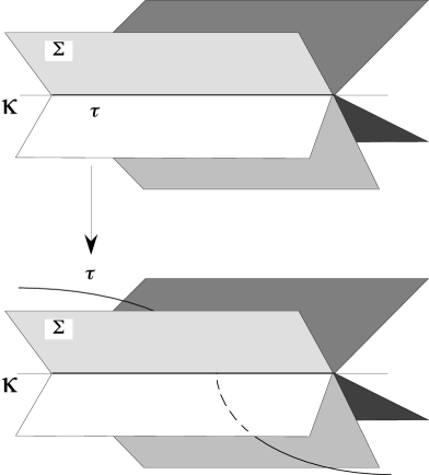
Figure 12: Isotopy of $\tau$ with respect to the spinal helix

Let $\kappa_{1}$ and $\kappa_{2}$ be two arcs such that $\kappa=\kappa_{1}\cup\kappa_{2}$ and $\kappa_{1}$ is isotoped to $K\cap W=\tau$ (see Figure 11). By capping off this spinal helix with $D$, we then obtain a standard spine $\Sigma$ of $Z$. Then we may isotope $\tau$, fixing $\partial\tau$ (see Figure 12) to intersect $\Sigma$ in a single point in $\kappa$. So $K$ intersects a standard spine exactly once, which is a contradiction with Lemma 5.1.

6 Proof of Theorem 1.4

Let $K$ be a non-standardly spinal knot in a lens space $L=L(m,n)$ with standard spine $\Sigma$, which yields $S^{3}$ by $\gamma$-Dehn surgery. A fortiori, $K$ is not a $0$ or $1$-bridge braid in $L$. Denote $s$ the minimal geometric intersection number between $K$ and $\Sigma$. Let $k=K_{\gamma}$ be the core of the $\gamma$-Dehn surgery in $S^{3}$. As we remark after Proposition 1.3 in the Introduction, we may assume that $k$ is not a torus knot. So there is an integer slope $r$ by [8] such that $r$-Dehn surgery on $k$ yields $L$. Then $H_{1}(L)=\mathbb{Z}/|r|\mathbb{Z}$ and $\Delta=\Delta(r,\lambda)=|r|=m\geq 2$.

Furthermore, since $K$ is neither $0$ nor $1$-bridge braid, we have $s\geq 3$ (Proposition 1.3), and hence by Theorem 4.1, we may assume that the essential thin presentation of $K$ begins by a local minimum.

So, let $\widehat{Q}$ be a level $2$-sphere between $\Sigma$ and the first local minimum and note $Q=\widehat{Q}\cap L_{K}$ the corresponding level surface.

And let $P$ be a Seifert surface (with minimal genus) for $k$, properly embedded in $L_{K}$. The single boundary component of $P$ has the longitudinal slope $\lambda$ and let denote $\widehat{P}$, the closed surface obtained by capping off $P$ by a disk.

Now, we consider the pair of intersection graphs $(G,H)$ of type $(\hbox{$\widehat{P}$},\hbox{$\widehat{Q}$})$.

Claim 6.1 The graphs $G$ and $H$ contain no trivial loop.

Proof.

Since $P$ is an incompressible and $\partial$-incompressible surface, then $H$ contains no trivial loop. And if $G$ contains a trivial loop, then we may assume (up to isotopy) that the tight presentation of $K$ begins by a local maximum, which is a contradiction. ∎

Let $G_{x}$ be the subgraph of $G$, with the single vertex and all the edges with an endpoint labelled by $x$. By the parity rule, the edges of $G_{x}$ do not have both endpoints labelled by $x$.

Claim 6.2

If $\Delta\geq 2g+1$ then $G_{x}$ contains at least two disk-faces.

Proof.

The Euler characteristic calculation for $G_{x}$ gives $\chi(\hbox{$\widehat{P}$})=2-2g=V-E+F$, where $V$ is the number of vertices, $E$ is the number of edges of $G_{x}$, and $\displaystyle F=\sum_{f\ face\ ofG_{x}}\chi(f)$. Here we have $V=1$ and $E=\Delta$, so $F=\Delta-2g+1$. Therefore, if $\Delta\geq 2g+1$ then $G_{x}$ contains at least two disk-faces. ∎

Each disk-face of $G_{x}$ contains a Scharlemann cycle in $G$, by [23, Lemma 2.2]. If $G$ contains a Scharlemann cycle of length $\ell$, then $X_{k}(r)$ contains a lens space of order $\ell$ (see [8] or below); therefore $\ell=m=|r|=\Delta$.

Assume for a contradiction that $\Delta\geq 2g+1$. Let $\sigma$ and $\sigma^{\prime}$ be two Scharlemann cycles in $G$. Without loss of generality, we may assume that $\{1,2\}$ are the labels of $\sigma$. Since $\sigma$ contains $\Delta$ edges, the corresponding edges in $H$ join the vertices $W_{1}$ and $W_{2}$, forming a connected component of $H$; i.e. no more edges than the $\Delta$’s from $\sigma$, can have its extremities attached on $W_{1}$ or $W_{2}$. Therefore, $\sigma^{\prime}$ has a pair of labels $\{n,n+1\}$ disjoint from $\{1,2\}$. And the vertices $W_{n}$, $W_{n+1}$, together with the corresponding edges of $\sigma^{\prime}$ form another connected component of $H$.

Let $\Lambda$ and $\Lambda^{\prime}$ be these components of $H$, corresponding to $\sigma$ and $\sigma^{\prime}$ respectively. Since $H$ is on a $2$-sphere, there exist two disjoint disks $D$ and $D^{\prime}$ in $\widehat{Q}$, containing $\Lambda$ and $\Lambda^{\prime}$ respectively.

Therefore $L=X_{k}(r)$ contains two disjoint punctured lens spaces.

Indeed, let $A,A^{\prime}$ be the face disks bounded by respectively $\sigma,\sigma^{\prime}$ in $G$; $V$ the $2$-handle of the attached solid torus between respectively $W_{1}$ and $W_{2}$ with no other $W_{i}$ inside, and similarly $V^{\prime}$ the $2$-handle of the attached solid torus between respectively $W_{n}$ and $W_{n+1}$ with no other $W_{i}$ inside. Then $N(D\cup A\cup V)$ and $N(D^{\prime}\cup A^{\prime}\cup V^{\prime})$ are two disjoint punctured lens spaces, in contradiction with $L$.

Consequently, $G$ contains at most one Scharlemann cycle. So $\Delta\leq 2g$.

Received:7 October 2002  Revised:2 May 2003

References

- [1] D. Bachman, Non-parallel essential surfaces in knots complements, preprint.
- [2] J. Bailey and D. Rolfsen, An unexpected surgery construction of a lens space, Pacific J. Math. 71 (1977), 295-298.
- [3] J. Berge, Some knots with surgeries yielding lens spaces, preprint.
- [4] J. Berge, The knots in which have nontrivial Dehn surgeries that yield , Top. and its App. 39 (1991), 1-19.
- [5] R.H. Bing, An alternative proof that all -manifolds can be triangulated, Ann. of Math. 69 (1959), 37-65.
- [6] S. Bleiler and R. Litherland, Lens spaces and Dehn surgery, Proc. Amer. Math. Soc. 107 (1989), 1127-1131.
- [7] J. Cerf, Sur les difféomorphismes de la sphère de dimension trois, Lecture Notes in Math. 53 Springer-Verlag, Berlin and New-York, 1968.
- [8] M. Culler, C.McA. Gordon, J. Luecke and P.B. Shalen, Dehn surgery on knots, Ann. of Math. 125 (1987), 237-300.
- [9] A. Deruelle, Conjecture de et nœuds minimalement tressés, preprint.
- [10] M. Domergue, Dehn surgery on a knot and real -projective space, Progress in knot theory and related topics (Travaux en cours 56) (Hermann, Paris 1997), 3-6.
- [11] M. Domergue and D. Matignon, Minimizing the boundaries of punctured projective planes in , J. of Knot Theory and Its Ram. 10 (2001), 415-430.
- [12] M. Eudave-Muñoz, Incompressible surfaces in tunnel number one knot complements, Topology Appl. 98 (1999), 167-189.
- [13] M. Eudave-Muñoz, Incompressible surfaces and -knots, preprint.
- [14] R. Fintushel and R. Stern, Constructing lens spaces by surgery on knots, Math. Z. 175 (1980), 33-51.
- [15] D. Gabai, Foliations and the topology of -manifolds, III, J. Diff. Geom. 26 (1987), 479-536.
- [16] D. Gabai, Surgery on knots in solid tori, Topology 28 (1989), 1-6.
- [17] H. Goda and M. Teragaito, Dehn surgeries on knots with yield lens spaces and genera of knots, Math. Proc. Camb. Phil. Soc. 129 (2000), 501-515.
- [18] C. McA. Gordon, Combinatorial methods in Dehn surgery, Lectures at Knots 96 (1997 World Scientific Publishing), 263-290.
- [19] C. McA. Gordon, Dehn surgery on knots, Proc. ICM Kyoto 1990 (1991), 555-590.
- [20] C. McA. Gordon, Dehn surgery and satellite knots, Trans. of the A.M.S. 275 (1983), 687-708.
- [21] C. McA. Gordon and R.A. Litherland, Incompressible planar surfaces in -manifolds, Top. and its App. 18 (1984), 121-144.
- [22] C. McA. Gordon and J. Luecke, Knots are determined by their complements, J. Amer. Math. Soc. 2 (1989), 385-409.
- [23] C. McA. Gordon and J. Luecke, Reducible manifolds and Dehn surgery, Topology 35 (1996), 94-101.
- [24] D. J. Heath and T. Kobayashi, Essential tangle decomposition from thin position of a link, Pacific J. Math. 179 (1997), 101-117.
- [25] J. A. Hoffman and D. Matignon, Producing essential -spheres, Top. and its App. 124 (2002), 435-444.
- [26] K. Ichihara, Exceptional surgeries and genera of knots, Proc. Japan Acad. Ser. A Math. Sci. 77 (2001), 66-67.
- [27] R. Lickorish, A representation of orientable combinatorial -manifolds, Ann. of. Math. 76 (1962), 531-540.
- [28] J. Luecke, Dehn surgery on knots in the -sphere, Proc. I.C.M. Zurich (1994).
- [29] S.V. Matveev, Complexity theory of three-dimensional manifolds, Acta Appl. Math. 19 (1990), 101-130.
- [30] D. Matignon and N. Sayari, Longitudinal slope and Dehn fillings, Hiroshima Math. Journal 33 (2003), 127-136.
- [31] E. Mo se, Affine structure in -manifolds, III, Ann. of Math. 55 (1952), 96-114.
- [32] L. Moser, Elementary surgery along a torus knot, Pacific J. of Math. 38 (1971), 737-745.
- [33] J.P. Neuwirth, Knot groups, Ann. of Math. Studies 56, Princeton University Press, New Jersey, 1965.
- [34] W. Parry, All types implies torsion, Proc. Amer. Math. Soc. 110 (1990), 871-875.
- [35] Y. Rieck and E. Sedgwick, Thin position for a connected sum of small knots, Alg. Geom. Top. 2 (2002), 297-309.
- [36] D. Rolfsen, Knots and Links, Math. Lect. Ser. 7, Publish or Perish, Berkeley, California, 1976.
- [37] M. Scharlemann and A. Thompson, Heegaard splittings of (surface) are standard, Math. Ann. 295 (1993), 549-564.
- [38] M. Teragaito, Cyclic surgery on genus one knots, Osaka J. of Math. 34 (1997), 145-150.
- [39] A. Thompson, Thin position and the recognition problem for the -sphere, Math. Research Letters. 1 (1994), 613-630.
- [40] A. Thompson, Thin position and bridge number for knots in the -sphere, Topology 36 (1997), 505-507.
- [41] A. Wallace, Modifications and cobounding manifolds, Can. J. Math. 12 (1960), 503-528.
- [42] S. Wang, Cyclic surgery on knots, Proc. Amer. Math. Soc. 107 (1989), 1091-1094.
- [43] Y.Q. Wu, Cyclic surgery and satellite knots, Topology Appl. 36 (1990), 205-208.
- [44] Y.Q. Wu, The reduciblility of surgered 3-manifolds, Topology Appl. 43 (1992), 213-218.
- [45] Y-Q. Wu, Thin position and essential planar surfaces, preprint.
Received:\qua7 October 2002 Revised:\qua2 May 2003