Nonisotopic symplectic tori in the fiber class of elliptic surfaces
Abstract. The purpose of this note is to present a construction of an infinite family of symplectic tori representing an arbitrary multiple of the homology class of the fiber of an elliptic surface , for , such that, for , there is no orientation-preserving diffeomorphism between and . In particular, these tori are mutually nonisotopic. This complements previous results of Fintushel and Stern in [FS2], showing in particular the existence of such phenomenon for a primitive class.
1. Introduction and statement of the result
An interesting question of symplectic topology concerns the existence, for a symplectic -manifold , of homologous, but not isotopic, symplectic representatives of a given homology class. Fintushel and Stern provided, in [FS2], the first example of such phenomenon. Their construction, that applies to a large class of symplectic manifolds, implies in particular that in any elliptic surface the class (where and is the class of the elliptic fiber) can be represented by an infinite family of mutually nonisotopic symplectic tori. Smith ([S1]) has been able to increase the genus of the examples, proving that the class (where ) in the (non simply-connected) surface can be represented by an infinite family of mutually nonisotopic symplectic curves (whose genus can be determined by the adjunction formula). The results above should be compared with the ones expected from a conjecture, due to Siebert and Tian, about the absence of such phenomena in the case of minimal rational ruled manifolds (Siebert and Tian have in fact proven the conjecture for several homology classes of and ).
These results leave open an interesting question, first pointed out by Smith in [S2]. Apart from the problem of obtaining examples for homology classes with odd divisibility, which appears mainly a technical question, the method used in [FS2] and [S1] does not allow us to obtain nonisotopy results for primitive homology classes, as the case of the fiber in .
Our purpose here is to present a different construction that produces families of symplectic tori also in primitive homology classes, and distinguishes their isotopy class avoiding the use of branched coverings. This allows us to extend (almost completely) the previous results, obtaining this way examples of symplectic surfaces homologous but not isotopic to a complex connected curve. Moreover, we will able to obtain a stronger result, namely that there does not exist a orientation-preserving diffeomorphism of sending one of these tori to another. Precisely, we will prove the following
Theorem 1.1.
For any there exists an infinite family of symplectic tori representing the class of an elliptic surface , for (where is the class of the fiber) such that, for , there is no orientation-preserving diffeomorphism between and . In particular, these tori are mutually nonisotopic.
We briefly sketch the argument: for each we will consider different homologous simple curves in the exterior of the -component link given by pushing off one component of the Hopf link. These curves will define a family of homologous, symplectic tori in the elliptic surface . We will glue copies of the rational elliptic surface along these tori. The symplectic manifolds obtained this way are link surgery manifolds, obtained by applying a variation of the construction of Fintushel-Stern (introduced in [V1]) to a family of links introduced in Section 2. Gluing along its fiber does not depend (up to diffeomorphism of the resulting manifolds) on the choice of the gluing map (see [GS]); in particular the resulting manifold depends only on the diffeomorphism type of the pair . Using different tori, we will get an infinite number of mutually nondiffeomorphic manifolds, distinguished (in a rather unusual way, see Section 4) by the SW invariant. For two such tori we have therefore no diffeomorphism of the pairs , . This implies in turn that the two tori are not smoothly isotopic.
We remark that while our examples cover cases that were excluded in [FS2] and, mutatis mutandis, in [S1], we have a price to pay, namely - as can be observed by analyzing the construction presented in the next section - the constraint of of Theorem 1.1 does not seem to be removable (while the examples of [FS2] exist for any elliptic surface).
2. Construction of the family of links
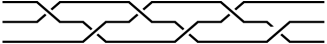
In this section we introduce a doubly-indexed class of links which we will be of paramount importance in our construction: First, denote by the -component link obtained by pushing off, with respect to the -framing, copies of one component of the Hopf link, (with the components oriented as the fibers of the Hopf fibration of ). Next, consider the -strand braid of Figure 1, and denote by be the -component link given by the -component link obtained by closing the braid of Figure 1, together with the braid axis oriented in such a way that the sublink composed by and any closed strand is the Hopf link.
Similarly, denote by the -component link given by the -component link obtained by closing the braid , the composition of copies of , together with the symmetry axis oriented as before.
The link is the link Borromean rings plus axis, analyzed (for different purposes) in [MT]. Its multivariable Alexander polynomial is
| (1) |
where is the variable corresponding to the meridian of the axis and correspond to the meridians of the three components given by the closure of the strands of the braid .
The link is defined by modifying in the following way; add, to the braid , strands, which are braided to the the first strand in the way denoted in Figure 2.

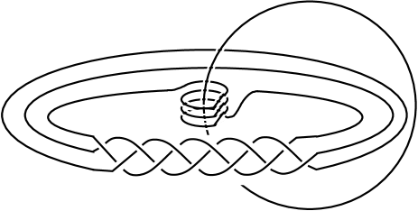
The closure of this new braid still gives the -component link (the various braids differ in fact only by Markov moves of type II), but if we add the axis , we get a new link , that we can visualize as obtained from by taking its first component and twisting it times around , see Figure 3.
The linking matrix of has the form
| (2) |
Observe that the linking matrix does not depend on .
We will not be interested in the computation of the complete multivariable Alexander polynomial of ; we will be content with the computation of the reduced polynomial , that is determined in the following
Lemma 2.1.
Let be a specialization of the Alexander polynomial of the link constructed before, for . Then
| (3) |
(with the convention that for the latter product is meant to be equal to ).
Proof: To prove this equation, we need first of all the Torres formula (see e.g. [Tu]) which in our case reads
| (4) |
where is the Alexander polynomial of and the are the linking numbers of Equation 2. To compute , we observe that is a periodic link, whose image under the action over with fixed point set the unknot is the Borromean rings ; from the formula for the Alexander polynomial of periodic links ([Tu]), and the fact that , we have
| (5) |
where is the primitive -th root of unit. Equation 1 and explicit calculation lead then to Equation 3. ∎
In the link , as for the Borromean rings , each component is an unknot, and any -component sublink is the trivial link. In particular, we can think at as the union where is the push-off of one component of the Hopf link (with the components and being unlinked). The links - for a fixed value of - differ therefore from the way the unknot is linked to the -component link . In particular, if we consider the link exterior , the link exteriors are obtained by removing nonisotopic circles. The case corresponds to the removal of the circle isotopic to , the meridian of . In the case of instead we are removing the circle which is homologous to in , as from the linking matrix of Equation 2 we deduce that has linking number with the axis , and with the other two components. In what follows we will consider the circle , as well as any other link component, endowed of the framing defined by a spanning disk.
3. Link surgery manifolds associated to
In this section we will construct the family of -manifolds used to prove Theorem 1.1. We start by recalling briefly the definition of link surgery manifold (see [FS1]), in the modified form introduced in [V1]. Consider an -component link and take an homology basis of simple curves of intersection in the boundary of the link exterior. Next, take elliptic surfaces and define the manifold
| (6) |
where the orientation reversing diffeomorphism between the boundary -tori is defined so to identify with and acts as complex conjugation on the remaining circle factor.
It is well known that in general the fiber sum above is not well defined and, for a fixed choice of homology basis, the smooth structure of the manifold above could depend on various choices, but because of the use of elliptic surfaces the manifold we will discuss will not be affected by this indeterminacy.
We have now a simple claim, whose proof follows by the definition of the elliptic surface as an iterated fiber sum of elliptic surfaces. Fix .
Claim 3.1.
Let be the -component link obtained by pushing off one copy of one component of the Hopf link; then we can chose the homology basis so that .
Proof: This claim follows from the observation that
| (7) |
so that choosing for and we have an explicit presentation of . ∎
In defined as above, the image of the class of the curve under the injective map
| (8) |
is the class of the elliptic fiber. More precisely, the image of the torus in is identified with a copy of the elliptic fiber .
Consider now the images of the tori under the injection
| (9) |
these compose a family of embedded, self-intersection zero framed tori. We have the following
Proposition 3.2.
Up to isotopy, the tori are symplectic submanifolds of , homologous to , where is the fiber of the elliptic fibration.
Proof: The statement on homology follows from the fact that the circles are all homologous to in , and the class coincides therefore with the image of under the map of Equation 8, i.e. it is the multiple of the class of the fiber.
In order to prove that the are symplectic, we will present , together with its symplectic structure, as a symplectic fiber sum in the following way: we perform a surgery with coefficients respectively to (i.e. ultimately a -surgery to the unknot ) to obtain the three manifold , in which the cores of the solid tori used in the surgery (specifically and itself, plus a curve isotopic to ) are framed, essential curves, whose framing induces one for the tori . Then we have
| (10) |
Note that, by the definition of fiber sum and because of the framings of , this construction coincides with the one of Claim 3.1.
In the curves are transverse to the fiber of the obvious fibration (which extends the fibration of ) and if we denote by a closed nondegenerate representative of that fibration, for any curve in which is transversal to the disk fibration, we have pointwise ; as a consequence, endowing of the symplectic structure (with a volume form on the fiber and sufficiently small), the tori (more generally, any torus as above) are symplectic in and, consequently, in . The curves are (up to isotopy) transverse to the disk fibration, and the tori are therefore symplectic. ∎
We can now introduce the link surgery manifolds associated to the links . These are defined as in Equation 6, but we can also present them as fiber sum of and along the embedded tori and . This is the content of the next definition, in which we write also the Seiberg-Witten polynomial of the manifold. Fix :
Definition 3.3.
Let be the -component link considered above, and define
| (11) |
where , for and . The SW polynomial is given by the product of the relative SW invariants
| (12) |
where is the symmetrized version of the multivariable Alexander polynomial.
The latter statement follows from Theorem 2.7 of [Ta] (see also [FS1]), as the homology class of the fiber of (the elliptic surface glued to (axis of )) is identified with the image of in .
Note that, although we made explicit a choice of curves in Definition 3.3, the smooth structure of the resulting manifold is independent of such choice, i.e. depends ultimately only on the diffeomorphism type of .
4. Infinitely many nonisotopic tori
In this section we will prove Theorem 1.1, namely we will show that, for a fixed value of , there are infinitely many diffeomorphism types of pairs . In order to prove that two tori , define different pairs for it would be sufficient to prove that the manifolds , have different SW polynomial. This means that there does not exist any automorphism of the manifold, inducing an automorphism of the second cohomology group which sends to (note that, when comparing the SW polynomials of two manifolds, as the ones appearing in Equation 12, we must consider the fact that the variables with the same symbol could refer to different cohomology classes for the two manifolds). Proving such a result appears to be quite a challenging problem (also considering the fact that we do not have a complete knowledge of the SW polynomials of our manifolds).
We will not attempt here to prove this, and we will limit ourselves to the proof of a weaker statement, that is anyhow sufficient to prove the statement of Theorem 1.1. The model of proof we will exploit here could find application also in other similar problems, where the explicit comparison of SW polynomials is difficult.
We will start, for sake of example, to work out in detail (and with a proof which differs from the general case) the case of two preferred tori, among the ones defined in Section 3, namely and . The proof that these tori define different pairs constitutes, in some sense, a “finite” version of Theorem 1.1. To obtain such a result, we will use in a rather weak way SW theory, building from the following observation: Let be the dimension of the the vector subspace of spanned by SW basic classes of ; then is a smooth invariant of . We use this fact to prove the following
Theorem 4.1.
For any the manifolds and are nondiffeomorphic (symplectic) manifolds.
Proof: in order to prove that, we will show that while . The first statement follows from the explicit computation of the Alexander polynomial of : we can observe that is a graph link obtained by connected sum along of a -component link given by the unknot and its cable with the -component link given by the unknot and two copies of the meridian. We leave to the reader the application of the results of [EN] to verify that the Alexander polynomial of this graph link is
| (13) |
(For similar computations see e.g. [V2].) In particular, this polynomial depends on only two variables, and the nonzero terms span a -dimensional subspace of . From this and Equation 12 the statement about follows. For , we can observe that the span of the nonzero terms of is bounded by below by the span of nonzero terms of the reduced polynomial which is given, according to Equation 4, by
| (14) |
The span of nonzero terms of this polynomial, as is easily verified, has dimension ; using Equation 12 again we obtain that (note that the fact that the SW polynomial reduced at is zero, for , does not affect this). This completes the proof. ∎
We will discuss now the general case. We will prove the following
Theorem 4.2.
For any the family contains an infinite number of nondiffeomorphic (symplectic) manifolds.
Proof: To prove this statement it is sufficient to prove that, if we denote by the number of basic classes of the manifold (for a fixed ), we have . We will start by proving this for the case of , where the invariant “coincides” with the Alexander polynomial of , as written in Equation 12. In this case we can observe that the number of basic classes of coincides with the number of nonzero terms in . Such a number is bounded by below by the number of nonzero terms in the reduced polynomial of Lemma 2.1, that we rewrite here by convenience:
| (15) |
In order to estimate we observe that the number of nonzero terms of a Laurent polynomial in satisfies the inequality of Lemma 5.1 in the appendix, i.e. where is the number of nonzero real roots of . The proof that will therefore prove our statement. It follows from elementary arguments that the equation has exactly real reciprocal solutions for , which differ for different values of . As a consequence each of the first factors appearing in the product of Equation 15 contributes two roots to , and we have
| (16) |
This proves the statement for .
We point out that the estimate on the number of terms is not optimal; in particular for odd it is not difficult to prove that .
To prove the statement for we consider the specialization of the SW polynomial given by
| (17) |
Once again, to prove that it is sufficient to prove that the number of nonzero terms in goes to infinity with . We can rewrite such a two-variable polynomial as
| (18) |
where, in the last identity, we define as the polynomial in that appears in writing as a power series in . If we consider the number of nonzero coefficients , this is bounded by below by the number of nonzero ; but the set of the latter coefficients (with a reparametrization for that takes account of the symmetrization and the “squaring” of the variable) coincides the set of the coefficients of Equation 15: therefore and Equation 16 asserts that this number diverges with . This completes the proof of the statement. ∎
Notice that, although implies , the condition is instead not sufficient to prove this, as we cannot guarantee that the specializations of the Alexander polynomials are the same.
As the family of manifolds obtained by gluing to along different , for a fixed , contains infinitely many nondiffeomorphic manifolds, infinitely many pairs are not diffeomorphic. In particular there are infinitely many nonisotopic symplectic tori . This completes the proof of Theorem 1.1.
5. Appendix
In this Appendix we give a proof of the Lemma used in Section 4. (It is likely that this statement already exists in literature, but we have not been able to find a reference). We thank Maximilian Seifert for suggesting us the proof of this Lemma.
Lemma 5.1.
Let be a nontrivial real Laurent polynomial. Denote by the number of nonzero real roots (counted without multiplicity) and by the number of terms of the polynomial. Then we have the inequality .
Proof: Assume first that is an ordinary polynomial of degree satisfying
| (19) |
and denote by the number of holes appearing in the polynomial plus , where we define by hole a string of consecutive powers with coefficient equal to zero and (e.g. has ). By obvious reasons, . Introduce now the family of integer pairs , with , defined in such a way that
| (20) |
this means that for some .
We will first prove, by induction over , that for a polynomial as in Equation 19 we have the inequality
| (21) |
This inequality is trivially true for . Assume by inductive hypothesis that it holds true for : we want to prove it for . Take the first derivatives of and denote
| (22) |
The polynomial has one hole less than and satisfies the conditions of Equation 19: we can thus apply the inductive hypothesis for it. Moreover, the roots of coincide with the roots of , plus the root : in particular we have
| (23) |
By Rolle’s theorem, the number of real zeroes of is bounded in terms of the zeroes of its derivative: more precisely we have, from Equation 23 and the fact that , the inequality
| (24) |
which is what we wanted to prove. This completes our induction.
Now we can observe that . Applying this to Equation 22, together with the inequality , proves the Lemma when is an ordinary polynomial. The statement for a general Laurent polynomials is readily obtained from this, by multiplying the polynomial with a suitable power of in order to get an ordinary polynomial of the form of Equation 19. ∎
Acknowledgements: I would like to thank Maximilian Seifert for the proof of Lemma 5.1. I would like to thank also Patrick Brosnan and Ki Heon Yun for discussions.
References
- [EN] D.Eisenbud, W.Neumann, Three Dimensional Link Theory and Invariants of Plane Curve Singularities, Annals of Mathematics Studies 110 (1985).
- [FS1] R.Fintushel, R.Stern, Knots, Links, and 4-manifolds, Invent.Math. 134, 363-400 (1998).
- [FS2] R.Fintushel, R.Stern, Symplectic Surfaces in a Fixed Homology Class, J. Differential Geom. 52, 203-222 (1999).
- [GS] R.Gompf, A.Stipsicz, 4-Manifolds and Kirby Calculus, Graduate Studies in Mathematics (vol. 20) AMS (1999).
- [MT] C.McMullen, C.Taubes, 4-Manifolds with Inequivalent Symplectic Forms and 3-Manifolds with Inequivalent Fibrations, Math.Res.Lett. 6, 681-696 (1999).
- [S1] I.Smith, Symplectic Submanifolds from Surface Fibrations, Pacif.Jour.Math. 198, 197-206 (2001).
- [S2] I.Smith, Review of [FS2], Math.Rev. 2001j:57036 (2001).
- [Ta] C.Taubes, The Seiberg-Witten Invariants and 4-manifolds with Essential Tori, Geom. & Topol. 5, 441-519 (2001).
- [Tu] V.Turaev, Reidemeister Torsion in Knot Theory, Russian Math.Surveys 41, 119-182 (1986).
- [V1] S.Vidussi, Smooth Structure on Some Symplectic Surfaces, Mich.Math.J. 49 (2001).
- [V2] S.Vidussi, Homotopy ’s with Several Symplectic Structures, Geom. & Topol. 5, 267-285 (2001).