Enumerative problems inspired by
Mayer’s theory of cluster integrals

Abstract

The basic functional equations for connected and 2-connnected graphs can be traced back to the statistical physicists Mayer and Husimi. They play an essential role in establishing rigorously the virial expansion for imperfect gases. We survey this approach and inspired by these equations, we investigate the problem of enumerating some classes of connected graphs all of whose blocks are contained in a given class $B$. Included are the species of Husimi graphs ($B=$ ”complete graphs”), cacti ($B=$ ”unoriented cycles”), and oriented cacti ($B=$ ”oriented cycles”). For each of these, we consider the question of their labelled or unlabelled enumeration and of their molecular expansion, according (or not) to their block-size distributions.

Résumé

Les équations fonctionnelles de base pour les graphes connexes et 2-connexes remontent aux physiciens Mayer et Husimi. Ces relations sont importantes pour établir rigoureusement le développement du viriel pour les gaz imparfaits. Nous présentons cette démarche et inspirés par ces relations, nous examinons le problème du dénombrement de quelques classes de graphes connexes dont les blocs sont pris dans une famille $B$ donnée. Cela inclut les graphes de Husimi ($B=$ ”graphes complets”), les cactus ($B=$ ”polygones”), et les cactus orientés ($B=$ ”cycles orientés”). Pour chacune de ces espèces, on s’intéresse au dénombrement étiqueté, ordinaire ou selon la distribution des tailles des blocs, au dénombrement non-étiqueté, et au développement moléculaire.

1 Introduction

1.1 Combinatorial species and functional equations for connected graphs and blocks

Informally, a combinatorial species is a class of labelled discrete structures which is closed under isomorphisms induced by relabelling along bijections. See Joyal [13] and Bergeron, Labelle, Leroux [2] for an introduction to the theory of species. To each species $F$ are associated a number of series expansions among which are the (exponential) generating function, $F(x)$, for labelled enumeration, defined by

$$F(x)=\sum_{n\geq 0}|F[n]|\frac{x^{n}}{n!},$$ (1)

where $|F[n]|$ denotes the number of $F$-structures on the set $[n]=\{1,2,\ldots,n\}$, the (ordinary) tilde generating function $\widetilde{F}(x)$, for unlabelled enumeration, defined by

$$\widetilde{F}(x)=\sum_{n\geq 0}\widetilde{F}_{n}{x^{n}},$$ (2)

where $\widetilde{F}_{n}$ denotes the number of isomorphism classes of F-structures of size $n$, the cycle index series $Z_{F}(x_{1},x_{2},x_{3},\cdots)$, defined by

$$Z_{F}(x_{1},x_{2},x_{3},\cdots)=\sum_{n\geq 0}\frac{1}{n!}\left(\sum_{\sigma\in S_{n}}\mathop{\rm fix}F[\sigma]\ x_{1}^{\sigma_{1}}x_{2}^{\sigma_{2}}x_{3}^{\sigma_{3}}\cdots\right),$$ (3)

where $S_{n}$ denotes the group of permutations of $[n]$, $\mathop{\rm fix}F[\sigma]$ is the number of $F$-structures on $[n]$ left fixed by $\sigma$, and $\sigma_{j}$ is the number of cycles of length $j$ in $\sigma$, and the molecular expansion of $F$, which is a description of the $F$-structures and a classification according to their stabilizers and will be discussed later.

Combinatorial operations are defined on species: sum, product, (partitional) composition, derivation, which correspond to the usual operations on the exponential generating functions. And there are rules for computing the other associated series, involving plethysm. See [2] for more details. An equality $F=G$ between species is a family of bijections between structures,

$$\alpha_{U}:F[U]\rightarrow G[U],$$

where $U$ ranges over all underlying (labelling) sets, which commutes under relabellings. Such an identity gives rise to an equality between all the series expansion associated to species.

Figure 1: A simple graph $g$ and its connected components

For example, the fact that any simple graph on a set (of vertices) $U$ is the disjoint union of connected simple graphs (see Figure 1) is expressed by the equation

$$\mathcal{G}=E(\mathcal{C}),$$ (4)

where $\mathcal{G}$ denotes the species of (simple) graphs, $\mathcal{C}$, that of connected graphs, and $E$, the species of Sets (in French: Ensembles). There correspond the well-known relations for their exponential generating functions,

$$\mathcal{G}(x)=\exp(\mathcal{C}(x))$$ (5)

and for their tilde generating functions,

$$\widetilde{\mathcal{G}}(x) = Z_{E}(\widetilde{\mathcal{C}}(x),\widetilde{\mathcal{C}}(x^{2}),\ldots)$$ (6)

$$= \exp{\left(\sum_{k\geq 1}\frac{1}{k}\widetilde{\mathcal{C}}(x^{k})\right)}.$$

Definitions. A cutpoint (or articulation point) of a connected graph $g$ is a vertex of $g$ whose removal yields a disconnected graph. A connected graph is called 2-connected if it has no cutpoint. A block in a simple graph is a maximal 2-connected subgraph. The block-graph of a graph $g$ is a new graph whose vertices are the blocks of $g$ and whose edges correspond to blocks having a common cutpoint. The block-cutpoint tree of a connected graph $g$ is a graph whose vertices are the blocks and the cutpoints of $g$ and whose edges correspond to incidence relations in $g$. See Figure 2.

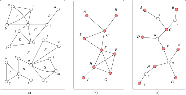
Figure 2: a) A connected graph $g$, b) the block-graph of $g$, c) the block-cutpoint tree of $g$

Now let $\mathcal{B}$ be a given species of 2-connected graphs. We denote by $C_{\mathcal{B}}$ the species of connected graphs all of whose blocks are in $\mathcal{B}$, called $C_{\mathcal{B}}$-graphs.

Examples 1.1. Here are some examples for various choices of $\mathcal{B}$:

1. If $\mathcal{B}=\mathcal{B}_{a}$, the class of all 2-connected graphs, then $C_{\mathcal{B}}=\mathcal{C}$, the species of (all) connected graphs.

2. If $\mathcal{B}=K_{2}$, the class of ”edges”, then $C_{\mathcal{B}}=\mbox{\Large{$a$}}$, the species of (unrooted, free) trees ($a$ for French arbres).

3. If $\mathcal{B}=\{P_{m},m\geq 2\}$, where $P_{m}$ denotes the class of size-$m$ polygons (by convention, $P_{2}=K_{2}$), then $C_{\mathcal{B}}=\mathop{\rm Ca}\nolimits$, the species of cacti. A cactus can also be defined as a connected graph in which no edge lies in more than one cycle. Figure 3, a), represents a typical cactus.

   

   Figure 3: a) a typical cactus, b) a typical oriented cactus

4. If $\mathcal{B}=K_{3}=P_{3}$, the class of ”triangles”, then $C_{\mathcal{B}}=\delta$, the class of triangular cacti.

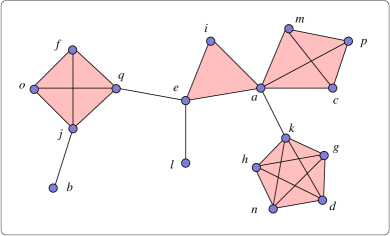
Figure 7: A Husimi graph with block-size distribution $(4,1,2,1,0,\ldots)$

5. If $\mathcal{B}=\{K_{n},n\geq 2\}$, the family of complete graphs, then $C_{\mathcal{B}}=\mathop{\rm Hu}\nolimits$, the species of Husimi graphs, that is of connected graphs whose blocks are complete graphs. They were first (informally) introduced by Husimi in [12]. A Husimi graph is shown in Figure 2, b). See also Figure 7. It can be easily shown that any Husimi graph is the block-graph of some connected graph.

6. If $\mathcal{B}=\{C_{n},n\geq 2\}$, the family of oriented cycles, then $C_{\mathcal{B}}=\mathop{\rm Oc}\nolimits$, the species of oriented cacti. Figure 3, b) shows a typical oriented cactus. These structures were introduced by C. Springer [28] in 1996. Although directed graphs are involved here, the functional equations (7) and (12) given below are still valid.

Remark. Cacti where first called Husimi trees. See for example [9], [11], [26] and [29]. However this term received much criticism since they are not necessarily trees. Also, a careful reading of Husimi’s article [12] shows that the graphs he has in mind and that he enumerates (see formula (42) below) are the Husimi graphs defined in item 5 above. The term cactus is now widely used. See Harary and Palmer [10]. Cacti appear regularly in the mathematical litterature, for example in the classification of base matroids [20], and in combinatorial optimization [4].

The following functional equation (see (7)) is fairly well known. It can be found in various forms and with varying degrees of generality in [2], [10], [13], [17], [18], [19], [24], [26], [27]. In fact, it was anticipated by the physicists (see [12] and [29]) in the context of Mayers’ theory of cluster integrals as we will see below. The form given here, in the structural language of species, is the most general one since all the series expansions follow. It is also the easiest form to prove.

Recall that for any species $F=F(X)$, the derivative $F^{\prime}$ of $F$ is the species defined as follows: an $F^{\prime}$-structure on a set $U$ is an $F$-structure on the set $U\cup\{\ast\}$, where $\ast$ is an external (unlabelled) element. In other words, one sets

$$F^{\prime}[U]=F[U+\{\ast\}].$$

Moreover, the operation $F\mapsto F^{\bullet}$, of pointing (or rooting) $F$-structures at an element of the underlying set, can be defined by

$$F^{\bullet}=X\cdot F^{\prime}.$$

Theorem 1.1

Let $\mathcal{B}$ be a class of 2-connected graphs and $C_{\mathcal{B}}$, the species of connected graphs all of whose blocks are in $\mathcal{B}$. We then have the functional equation

$$C_{\mathcal{B}}^{\prime}=E(\mathcal{B}^{\prime}(C_{\mathcal{B}}^{\bullet})).$$ (7)

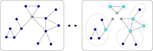
Figure 4: $C_{\mathcal{B}}^{\prime}=E(\mathcal{B}^{\prime}(C_{\mathcal{B}}^{\bullet}))$

Proof. See Figure 4. $\Box$

Multiplying (7) by $X$, one finds

$$C_{\mathcal{B}}^{\bullet}=X\cdot E(\mathcal{B}^{\prime}(C_{\mathcal{B}}^{\bullet})),$$ (8)

and, for the exponential generating function,

$$C_{\mathcal{B}}^{\bullet}(x)=x\cdot\exp(\mathcal{B}^{\prime}(C_{\mathcal{B}}^{\bullet}(x))).$$ (9)

1.2 Weighted versions

Weighted versions of these equations are needed in the applications. See for example Uhlenbeck and Ford [29]. A weighted species is a species $F$ together with weight functions $w=w_{U}:F[U]\rightarrow{\sf IK}$ defined on $F$-structures, which commute with the relabellings. Here ${\sf IK}$ is a commutative ring in which the weights are taken, usually a ring of polynomials or formal power series over a field of characteristic zero. We write $F=F_{w}$ to emphasize the fact that $F$ is a weighted species with weight function $w$. The associated generating functions are then adapted by replacing set cardinalities $|A|$ by total weights

$$|A|_{w}=\sum_{a\in A}w(a).$$

The basic operations on species are also adapted to the weighted context, using the concept of Cartesian product of weighted sets: Let $(A,u)$ and $(B,v)$ be weighted sets. A weight function $w$ is defined on the Cartesian product $A\times B$ by

$$w(a,b)=u(a)\cdot v(b).$$

We then have    $|A\times B|_{w}=|A|_{u}\cdot|B|_{v}$.

Definition. A weight function $w$ on the species $\mathcal{G}$ of graphs is said to be multiplicative on the connected components if for any graph $g\in\mathcal{G}[U]$, whose connected components are $c_{1},c_{2},\ldots,c_{k}$, we have

$$w(g)=w(c_{1})w(c_{2})\cdots w(c_{k}).$$

Examples 1.2. The following weight functions $w$ on the species of graphs are multiplicative on the connected components.

1. $w_{1}(g):=y^{e(g)}$, where $e(g)$ is the number of edges of $g$.

2. $w_{2}(g)$ = graph complexity of $g$ := number of maximal spanning forests of $g$.

3. $w_{3}(g):=x_{0}^{n_{0}}x_{1}^{n_{1}}x_{2}^{n_{2}}\cdots$, where $n_{i}$ is the number of vertices of degree $i$.

Theorem 1.2

Let $w$ be a weight function on graphs which is multiplicative on the connected components. Then we have

$$\mathcal{G}_{w}=E\left(\mathcal{C}_{w}\right).$$ (10)

For the exponential generating functions, we have

$$G_{w}(x)=\exp(\mathcal{C}_{w}(x)),$$

where $G_{w}(x)\ =\ \sum_{n\geq 0}|\mathcal{G}[n]|_{w}\frac{x^{n}}{n!}\ =\ \sum_{n\geq 0}(\sum_{g\in G[n]}w(g))\frac{x^{n}}{n!},$ and similarly for $\mathcal{C}_{w}(x).$

Definition. A weight function on connected graphs is said to be block-multiplicative if for any connected graph $c$, whose blocks are $b_{1},b_{2},\ldots,b_{k}$, we have

$$w(c)=w(b_{1})w(b_{2})\cdots w(b_{k}).$$

Examples 1.3. The weight functions $w_{1}(g)=y^{e(g)}$ and   $w_{2}(g)=$ graph complexity of $g$ of Examples 1.2 are block-multiplicative, but not the function $w_{3}(g)=x_{0}^{n_{0}}x_{1}^{n_{1}}x_{2}^{n_{2}}\cdots$. Another example of a block-multiplicative weight function is obtained by introducing formal variables $y_{i}$ ($i\geq 2$) marking the block sizes. In other terms, if the connected graph $c$ has $n_{i}$ blocks of size $i$, for $i=2,3,\ldots$, one sets

$$w(c)=y_{2}^{n_{2}}y_{3}^{n_{3}}\cdots.$$ (11)

The following result is then simply the weighted version of Theorem 1.1.

Theorem 1.3. Let $w$ be a block-multiplicative weight function on connected graphs whose blocks are in a given species $B$. Then we have

$$\left({C_{\mathcal{B}}^{\bullet}}\right)_{w}=X\cdot E(\mathcal{B}^{\prime}_{w}((C_{\mathcal{B}}^{\bullet})_{w})).$$ (12)

1.3 Outline

In the next section, we see how equations (10) and (12) are involved in the thermodynamical study of imperfect (or non ideal) gases, following Mayers’ theory of cluster integrals [21], as presented in Uhlenbeck and Ford [29]. In particular, the virial expansion, which is a kind of asymptotic refinement of the perfect gases law, is established rigourously, at least in its formal power series form. See equation (34) below. It is amazing to realize that the coefficients of the virial expansion involve directly the total valuation $|\mathcal{B}_{a}[n]|_{w}$, for $n\geq 2$, of 2-connected graphs. An important role in this theory is also played by the enumerative formula (42) for labelled Husimi trees according to their block-size distribution, which extends Cayley’s formula $n^{n-2}$ for the number of labelled trees of size $n$.

Motivated by this, we first consider, in Section 3, the labelled enumeration of some classes of connected graphs of the form $C_{\mathcal{B}}$, according or not to their block-size distribution. Included are the species of Husimi graphs, cacti, and oriented cacti. The methods involve the Lagrange inversion formula and Prüfer-type bijections. It is also natural to examine the question of unlabelled enumeration of these structures. This is a more difficult problem, for two reasons. First, equation (12) deals with rooted structures and it is necessary to introduce a tool for counting the unrooted ones. Traditionally, this is done by extending the Dissimilarity charactistic formula for trees of Otter [25]. See for example [9]. Inspired by formulas of Norman ([6], (18)) and Robinson ([27], Theorem 7), we have given over the years a more structural formula which we call the Dissymmetry theorem for graphs, whose proof is remarkably simple and which can esily be adapted to various classes of tree-like structures; see [2], [3], [7], [14], [15], [16], [18], [19]. Second, as for trees, it should not be expected to obtain simple closed expressions but rather recurrence formulas for the number of unlabelled $C_{\mathcal{B}}$-structures. Three examples are given in that section.

Finally, in Section 4, we present the molecular expansion of some of these species. This expansion can be computed first for the rooted species, by iteration, and the dissymmetry theorem is then invoked for the unrooted ones. The computations can be carried out easily using the Maple package ”Devmol” developped at LaCIM and available at the URL www.lacim.uqam.ca; see [1].

Acknowledgements. This talk is partly taken from my student Mélanie Nadeau’s ”Mémoire de maîtrise” [23]. I would like to thank her and Pierre Auger for their considerable help, and also Abdelmalek Abdesselam, André Joyal, Gilbert Labelle, Bob Robinson, and Alan Sokal, for useful discussions.

2 Some statistical mechanics

2.1 Partition functions for the non-ideal gas

Consider a non-ideal gas, formed of $N$ particles interacting in a vessel $V\subseteq{\sf IR}^{3}$ (whose volume is also denoted by $V$) and whose positions are $\overrightarrow{x_{1}},\overrightarrow{x_{2}},\ldots,\overrightarrow{x_{N}}$. The Hamiltonian of the system is of the form

$$H=\sum_{i=1}^{N}\left(\frac{\overrightarrow{p_{i}}^{2}}{2m}+U(\overrightarrow{x_{i}})\right)+\sum_{1\leq i<j\leq N}\varphi(|\overrightarrow{x_{i}}-\overrightarrow{x_{j}}|),$$ (13)

where $\overrightarrow{p_{i}}$ is the linear momentum vector and $\frac{\overrightarrow{p_{i}}^{2}}{2m}$ is the kinetic energy of the $i^{th}$ particle, $U(\overrightarrow{x_{i}})$ is the potential at position $\overrightarrow{x_{i}}$ due to outside forces (e.g., walls), $|\overrightarrow{x_{i}}-\overrightarrow{x_{j}}|=r_{ij}$ is the distance between the particles $\overrightarrow{x_{i}}$ and $\overrightarrow{x_{j}}$, and it is assumed that the particles interact only pairwise through the central potential $\varphi(r)$. This potential function $\varphi$ has a typical form shown in Figure 5 a).

Figure 5: a) the function $\varphi(r)$, b) the function $f(r)$

The canonical partition function $Z(V,N,T)$ is defined by

$$Z(V,N,T)=\frac{1}{N!h^{3N}}\int\exp{(-\beta H)}d\Gamma,$$ (14)

where $h$ is Planck’s constant, $\beta={1\over{kT}}$, $T$ is the absolute temperature and $k$ is Boltzmann’s constant, and $\Gamma$ represents the state space $\overrightarrow{x_{1}},\ldots,\overrightarrow{x_{N}},\overrightarrow{p_{1}},\ldots,\overrightarrow{p_{N}}$ of dimension $6N$. A first simplification comes from the assumption that the potential energy $U(\overrightarrow{x_{i}})$ is negligible or null. Secondly, the integral over the momenta $\overrightarrow{p_{i}}$ in (14) is a product of Gaussian integrals which are easily evaluated so that the canonical partition function can now be written as

$$Z(V,N,T)=\frac{1}{N!\lambda^{3N}}\int_{V}\cdots\int_{V}\exp{\left(-\beta\sum_{i<j}\varphi(|\overrightarrow{x_{i}}-\overrightarrow{x_{j}}|)\right)}d\overrightarrow{x_{1}}\cdots d\overrightarrow{x_{N}},$$ (15)

where $\lambda=h(2\pi mkT)^{-\frac{1}{2}}$.

Mathematically, the grand-canonical distribution is simply the generating function for the canonical partition functions, defined by

$$Z_{\mathop{\rm gr}}(V,T,z)=\sum_{N=0}^{\infty}Z(V,N,T)(\lambda^{3}z)^{N},$$ (16)

where the variable $z$ is called the fugacity or the activity. All the macroscopic parameters of the system are then defined in terms of this grand canonical ensemble. For example, the pressure, $P$, the average number of particles, $\overline{N}$, and the density, $\rho$, are defined by

$$\frac{P}{kT}=\frac{1}{V}\log{Z_{\mathop{\rm gr}}(V,T,z)},\ \ \ \overline{N}=z\frac{\partial}{\partial z}\log{Z_{\mathop{\rm gr}}(V,T,z)},\ \ \ \mathrm{and}\ \ \ \rho:=\frac{\overline{N}}{V}.$$ (17)

2.2 The virial expansion

In order to better explain the thermodynamic behaviour of non ideal gases, Kamerlingh Onnes proposed, in 1901, a series expansion of the form

$$\frac{P}{kT}=\frac{\overline{N}}{V}+\gamma_{2}(T)\left(\frac{\overline{N}}{V}\right)^{2}+\gamma_{3}(T)\left(\frac{\overline{N}}{V}\right)^{3}+\cdots,$$ (18)

called the virial expansion. Here $\gamma_{2}(T)$ is the second virial coefficient, $\gamma_{3}(T)$ the third, etc. This expansion was first derived theoretically from the partition function $Z_{\mathop{\rm gr}}$ by Mayer [21] around 1930. It is the starting point of Mayer’s theory of ”cluster integrals”. Mayer’s idea consists in setting

$$1+f_{ij}=\exp{\left(-\beta\varphi(|\overrightarrow{x_{i}}-\overrightarrow{x_{j}}|)\right)},$$ (19)

where $f_{ij}=f(r_{ij})$. The general form of the function $f(r)=\exp(-\beta\varphi(r))-1$ is shown in Figure 5, b). In particular, $f(r)$ vanishes when $r$ is greater than the range $r_{1}$ of the interaction potential. By substituting in the canonical partition function (15), one obtains

$$Z(V,N,T)=\frac{1}{N!\lambda^{3N}}\int_{V}\cdots\int_{V}\prod_{1\leq i<j\leq N}\left(1+f_{ij}\right)d\overrightarrow{x_{1}}\cdots d\overrightarrow{x_{N}}.$$ (20)

The terms obtained by expanding the product $\prod_{1\leq i<j\leq N}(1+f_{ij})$ can be represented by simple graphs where the vertices are the particles and the edges are the chosen factors $f_{ij}$. The partition function (20) can then be rewritten in the form

$$Z(V,N,T) = \frac{1}{N!\lambda^{3N}}\sum_{g\in\mathcal{G}[N]}\int_{V}\cdots\int_{V}\prod_{\{i,j\}\in g}f_{ij}\ d\overrightarrow{x_{1}}\cdots d\overrightarrow{x_{N}}$$ (21)

$$= \frac{1}{N!\lambda^{3N}}\sum_{g\in\mathcal{G}[N]}W(g),$$

where the weight $W(g)$ of a graph $g$ is given by the integral

$$W(g)=\int_{V}\cdots\int_{V}\prod_{\{i,j\}\in g}f_{ij}d\overrightarrow{x_{1}}\cdots d\overrightarrow{x_{N}}.$$ (22)

For the grand canonical function, we then have

$$Z_{\mathop{\rm gr}}(V,T,z) = \sum_{N=0}^{\infty}Z(V,N,T)(\lambda^{3}z)^{N}$$ (23)

$$= \sum_{N=0}^{\infty}\frac{1}{N!\lambda^{3N}}\sum_{g\in\mathcal{G}[N]}W(g)(\lambda^{3}z)^{N}$$

$$= \sum_{N=0}^{\infty}\frac{1}{N!}\sum_{g\in\mathcal{G}[N]}W(g)z^{N}$$

$$= \mathcal{G}_{W}(z).$$

Proposition 2.1

The weight function $W$ is multiplicative on the connected components.

For example, for the graph $g$ of Figure 1, we have

$$W(g)=\int_{V^{8}}f_{12}f_{17}f_{27}f_{45}f_{46}f_{56}f_{58}d\overrightarrow{x_{1}}\cdots d\overrightarrow{x_{8}}$$

$$= \int f_{12}f_{17}f_{27}d\overrightarrow{x_{1}}d\overrightarrow{x_{2}}d\overrightarrow{x_{7}}\int d\overrightarrow{x_{3}}\int f_{45}f_{46}f_{56}f_{58}d\overrightarrow{x_{4}}d\overrightarrow{x_{5}}d\overrightarrow{x_{6}}d\overrightarrow{x_{8}}$$

$$= W(c_{1})W(c_{2})W(c_{3}),$$

where $c_{1}$, $c_{2}$ and $c_{3}$ represent the three connected components of $g$. Following Theorem 1.2, we deduce that

$$\mathcal{G}_{W}(z)=\exp{\left(\mathcal{C}_{W}(z)\right)},$$ (24)

where $\mathcal{C}_{W}$ denotes the weighted species of connected graphs, with

$$\mathcal{C}_{W}(z)=\sum_{n\geq 1}|\mathcal{C}[n]|_{W}\frac{z^{n}}{n!},$$

and

$$|\mathcal{C}[n]|_{W}=\sum_{c\in\mathcal{C}[n]}\int_{V}\cdots\int_{V}\prod_{\{i,j\}\in c}f_{ij}\ d\overrightarrow{x_{1}}\cdots d\overrightarrow{x_{n}}.$$ (25)

Historically, the quantities $b_{n}(V)=\frac{1}{Vn!}|\mathcal{C}[n]|_{W}$ are precisely the cluster integrals of Mayer. Equation (24) then provides a combinatorial interpretation for the quantity $\frac{P}{kT}$. Indeed, one has, by (17),

$$\frac{P}{kT} = \frac{1}{V}\log{Z_{\mathop{\rm gr}}(V,T,z)}$$ (26)

$$= \frac{1}{V}\log{\mathcal{G}_{W}(z)}$$

$$= \frac{1}{V}\mathcal{C}_{W}(z).$$

Proposition 2.2

For $V$ large, the weight function $w(c)=\frac{1}{V}W(c)$, defined on the species of connected graphs, is block-multiplicative.

Proof. First observe that for any connected graph $c$ on the set of vertices $[k]=\{1,2,\ldots\,k\}$, the value of the partial integral

$$I=I(\overrightarrow{x_{k}})=\lim_{V\rightarrow\infty}\,\int_{V}\cdots\int_{V}\prod_{\{i,j\}\in c}f_{ij}d\overrightarrow{x_{1}}\cdots d\overrightarrow{x_{k-1}}$$ (27)

is in fact independent of $\overrightarrow{x_{k}}$. Indeed, since the $f_{ij}$’s only depend on the relative positions $r_{ij}=|\overrightarrow{x_{i}}-\overrightarrow{x_{j}}|,$ and considering the short range $r_{1}$ of the interaction potential and the connectednes of $c$, we see that the support of the integrand in (27) lies in a ball of radius at most $(k-1)r_{1}$ centered at $\overrightarrow{x_{k}}$ and that a simple translation $\overrightarrow{x_{i}}\mapsto\overrightarrow{x_{i}}+\overrightarrow{u}$ will give the same value of the integral. It follows that

$$W(c) = \int_{V}\cdots\int_{V}\prod_{\{i,j\}\in c}f_{ij}d\overrightarrow{x_{1}}\cdots d\overrightarrow{x_{k-1}}\int_{V}d\overrightarrow{x_{k}}$$

$$\approx \int_{V}\cdots\int_{V}\prod_{\{i,j\}\in c}f_{ij}d\overrightarrow{x_{1}}\cdots d\overrightarrow{x_{k-1}}\cdot V,$$

for $V$ large, and the value of the partial integral (27) is in fact $w(c)$:

$$\lim_{V\rightarrow\infty}\,\int_{V}\cdots\int_{V}\prod_{\{i,j\}\in c}f_{ij}d\overrightarrow{x_{1}}\cdots d\overrightarrow{x_{k-1}}=\lim_{V\rightarrow\infty}\,\frac{1}{V}W(c)=w(c).$$ (28)

Now if a connected graph is decomposed into blocks $b_{1},b_{2},\ldots,b_{k}$, we have

$$w(c)=w(b_{1})w(b_{2})\cdots w(b_{k}).$$

For example, for the graph $c$ shown in Figure 6, we have

$$w(c)=\int_{V^{7}}f_{12}f_{13}f_{23}f_{34}f_{56}f_{37}f_{36}f_{67}f_{68}f_{78}d\overrightarrow{x_{1}}d\overrightarrow{x_{2}}\cdots d\overrightarrow{x_{7}}$$

$$= \int f_{12}f_{13}f_{23}d\overrightarrow{x_{1}}d\overrightarrow{x_{2}}\,f_{34}d\overrightarrow{x_{4}}\,f_{56}d\overrightarrow{x_{5}}\,f_{37}f_{36}f_{67}f_{68}f_{78}d\overrightarrow{x_{3}}d\overrightarrow{x_{6}}d\overrightarrow{x_{7}}$$

$$= w(b_{1})w(b_{2})w(b_{3})w(b_{4}).$$

$\Box$

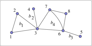
Figure 6: A connected graph with blocks $b_{1},b_{2},b_{3},b_{4}$

By Theorem 1.3, it follows that

$$\mathcal{C}_{w}^{\bullet}=X\cdot E(\mathcal{B}^{\prime}_{w}(\mathcal{C}_{w}^{\bullet})),$$ (29)

where $\mathcal{B}=\mathcal{B}_{a}$ is the species of all 2-connected graphs, and for the exponential generating functions,

$$\mathcal{C}_{w}^{\bullet}(z)=z\exp(\mathcal{B}^{\prime}_{w}(\mathcal{C}_{w}^{\bullet}(z))).$$ (30)

2.3 Computation of the virial expansion

The virial expansion (18) can now be established, following Uhlenbeck and Ford [29]. From (17), we have, for the density $\rho(z)=\frac{\overline{N}}{V}$,

$$\rho(z) = z\frac{\partial}{\partial z}\frac{1}{V}\log{Z_{\mathop{\rm gr}}(V,T,z)}$$ (31)

$$= z\frac{\partial}{\partial z}\mathcal{C}_{w}(z)$$

$$= \mathcal{C}_{w}^{\bullet}(z).$$

Hence $\rho(z)$ satisfies the functional equation (30), that is

$$\rho(z)=z\exp{\mathcal{B}^{\prime}_{w}(\rho(z))}.$$ (32)

The idea is then to use this relation in order to express $z$ in terms of $\rho$ in $\frac{P}{kT}(z)$, as follows. We have, by (26) and (31),

$$\frac{P}{kT} = \frac{1}{V}\log{Z_{\mathop{\rm gr}}(V,T,z)}$$ (33)

$$= \mathcal{C}_{w}(z)$$

$$= \int_{0}^{z}\mathcal{C}_{w}^{\prime}(t)\ dt$$

$$= \int_{0}^{z}\frac{\rho(t)}{t}\ dt.$$

Let us make the change of variable

$$t=t(r)=r\exp{(-\mathcal{B}_{w}^{\prime}(r))},$$

which is the inverse function of $r=\rho(t)$, by (32). Note that $\rho(0)=0$ and $\rho(z)=\rho$, and also that

$$dt=[\exp{(-\mathcal{B}_{w}^{\prime}(r))}-r\exp{(-\mathcal{B}_{w}^{\prime}(r))}\cdot\mathcal{B}_{w}^{\prime\prime}(r)]dr.$$

Pursuing the computation of the integral (33), we have

$$\frac{P}{kT} = \int_{0}^{z}\frac{\rho(t)}{t}\ dt$$ (34)

$$= \int_{0}^{\rho}\left(1-r\mathcal{B}_{w}^{\prime\prime}(r)\right)\ dr$$

$$= \rho-\int_{0}^{\rho}r\mathcal{B}_{w}^{\prime\prime}(r)\ dr$$

$$= \rho-\int_{0}^{\rho}\sum_{n\geq 1}n\beta_{n+1}\frac{r^{n}}{n!}\ dr$$

$$= \rho-\sum_{n\geq 2}(n-1)\beta_{n}\frac{{\rho}^{n}}{n!},$$

where we have set $\mathcal{B}_{w}(r)=\sum_{n\geq 2}\beta_{n}\frac{r^{n}}{n!}$. This is precisely the virial expansion, with $\rho=\frac{\overline{N}}{V}$. Hence the $n^{\mathop{\rm th}}$ virial coefficient, for $n\geq 2$, is given by

$$\gamma_{n}(T) = -\frac{(n-1)}{n!}\beta_{n}$$ (35)

$$= -\frac{(n-1)}{n!}|\mathcal{B}[n]|_{w}.$$

Mayer’s original proof of the virial expansion is more technical, since he is not aware of a direct combinatorial proof of equation (30). The following observation is used: By grouping the connected graphs on $[n]$ whose block decomposition determines the same Husimi graph on $[n]$, and then collecting all Husimi graphs having the same block-size distribution, one obtains, using the 2-multiplicativity of $w$,

$$|C[n]|_{w} = \sum_{c\in\mathcal{C}[n]}w(c)$$

$$= \sum_{\{B_{1},B_{2},\ldots\}\in\mathop{\rm Hu}\nolimits[n]}\sum_{\{b_{i}\in\mathcal{B}[B_{i}]\}}\prod_{i}w(b_{i})$$

$$= \sum_{\{B_{1},B_{2},\ldots\}\in\mathop{\rm Hu}\nolimits[n]}\prod_{i}\sum_{b\in\mathcal{B}[B_{i}]}w(b)$$

$$= \sum_{\{B_{1},B_{2},\ldots\}\in\mathop{\rm Hu}\nolimits[n]}\prod_{i}\beta_{|B_{i}|}$$

$$= \sum_{{n_{2},n_{3},\ldots\atop\sum n_{i}(i-1)=n-1}}\mathop{\rm Hu}\nolimits(n_{2},n_{3},\ldots)\beta_{2}^{n_{2}}\beta_{3}^{n_{3}}\cdots,$$

where $\mathop{\rm Hu}\nolimits[n]$ denotes the set of Husimi graphs on $[n]$ and $\mathop{\rm Hu}\nolimits(n_{2},n_{3},\ldots)$ is the number of Husimi graphs on $[n]$ having $n_{i}$ blocks of size $i$, for $i\geq 2$. Mayer then proves the following enumerative formula

$$\mathop{\rm Hu}\nolimits(n_{2},n_{3},\ldots)=\frac{(n-1)!\,n^{\sum n_{j}-1}}{\prod_{i\geq 2}\,(i-1)!^{n_{i}}\,n_{i}!},$$ (36)

and goes on proving (30) and (34) analytically.

Formula (36) is quite remarkable. It is an extension of Cayley’s formula $n^{n-2}$ for the number of trees on $[n]$ (take $n_{2}=n-1,n_{3}=0,\ldots$). It has many different proofs, using, for example, Lagrange inversion or a Prüfer correspondence, and gives the motivation for the enumerative problems related to Husimi graphs, cacti, and oriented cacti, studied in the next section.

2.4 Gaussian model

It is interesting, mathematically, to consider a Gaussian model, where

$$f_{ij}=-\exp{(-\alpha||\overrightarrow{x_{i}}-\overrightarrow{x_{j}}||^{2})},$$ (37)

which corresponds to a soft repulsive potential, at constant temperature. In this case, all cluster integrals can be explicitly computed (see [29]): The weight $w(c)$ of a connected graph $c$, defined by (28), has value

$$w(c)=(-1)^{e(c)}\left(\frac{\pi}{\alpha}\right)^{\frac{3}{2}(n-1)}\gamma(c)^{-\frac{3}{2}},$$ (38)

where $e(c)$ is the number of edges of $c$ and $\gamma(c)$ is the graph complexity of $c$, that is, the number of spanning subtrees of $c$. This formula incorporates three very descriptive weightings on connected graphs, which are multiplicative on 2-connected components, namely,

$$w_{1}(c)=y^{e(c)},\ \ w_{2}(c)=\gamma(c),$$

already seen in Examples 1.2, and $w_{3}(c)=u^{n-1},$ where $n$ is the number of vertices.

3 Enumerative results

In this section, we investigate the enumeration of Husimi graphs, cacti and oriented cacti, according, or not, to their block size distribution. Recall that these classes can be viewed as species of connected graphs of the form $C_{\mathcal{B}}$ and that the functional equation (8) for rooted $C_{\mathcal{B}}$-structures can be invoked, as well as its weighted version (12).

3.1 Labelled enumeration

Proposition 3.1

The number $\mathop{\rm H}\nolimits_{n}=|\mathop{\rm Hu}\nolimits[n]|$ of (labelled) Husimi graphs on $[n]$, for $n\geq 1$, is given by

$$\mathop{\rm H}\nolimits_{n}=\sum_{k\geq 0}S(n-1,k)\,n^{k-1},$$ (39)

where $k$ represents the number of blocks and $S(m,k)$ denotes the Stirling number of the second kind.

Proof. The species $\mathop{\rm Hu}\nolimits$ of Husimi graphs is of the form $C_{\mathcal{B}}$ with $\mathcal{B}=K_{\geq 2}$, the class of complete graphs of size $\geq 2$. From the species point of view, it is equivalent to take $\mathcal{B}=E_{\geq 2}$, the species of sets of size $\geq 2$. We then have $\mathcal{B}^{\prime}=E_{\geq 1}$, with exponential generating function $E_{\geq 1}(x)={e^{x}-1}$. Hence the species $\mathop{\rm Hu}\nolimits^{\bullet}$ of rooted Husimi graphs satisfies the functional equation

$$\mathop{\rm Hu}\nolimits^{\bullet}=X\,E(E_{\geq 1}(\mathop{\rm Hu}\nolimits^{\bullet})).$$ (40)

which, for the generating function $\mathop{\rm Hu}\nolimits^{\bullet}(x)$, translates into

$$\mathop{\rm Hu}\nolimits^{\bullet}(x)=xR(\mathop{\rm Hu}\nolimits^{\bullet}(x)),$$ (41)

with $R(x)=\exp(e^{x}-1)$. The Lagrange inversion formula then gives

$$[x^{n}]\mathop{\rm Hu}\nolimits^{\bullet}(x) = \frac{1}{n}[t^{n-1}]\left(e^{e^{t}-1}\right)^{n}$$

$$= \frac{1}{n}[t^{n-1}]e^{n(e^{t}-1)}$$

$$= \frac{1}{n}[t^{n-1}]\sum_{k\geq 0}n^{k}\frac{(e^{t}-1)^{k}}{k!}$$

$$= \frac{1}{n}[t^{n-1}]\sum_{k\geq 0}n^{k}\sum_{m}S(m,k)\frac{t^{m}}{m!}$$

$$= \frac{1}{n}\sum_{k\geq 0}n^{k}\frac{S(n-1,k)}{(n-1)!}$$

$$= \sum_{k\geq 0}n^{k}\frac{S(n-1,k)}{n!}.$$

Since we are dealing with exponential generating functions, we should multiply by $n!$ to get the coefficient of $x^{n}\over n!$. Moreover we should divide by $n$ to obtain the number of unrooted Husimi graphs. In conclusion, we have $\mathop{\rm H}\nolimits_{n}=\frac{1}{n}n![x^{n}]\mathop{\rm Hu}\nolimits^{\bullet}(x)=\sum_{k\geq 0}S(n-1,k)\,n^{k-1}.$ The fact that $k$ represents the number of blocks will appear more clearly in the bijective proof given below. $\Box$

We now come to Mayer’s enumerative formula (36).

Proposition 3.2

(Mayer [22], Husimi [12]) Let $(n_{2},n_{3},\ldots)$ be a sequence of non-negative integers and $n=\sum_{i\geq 2}n_{i}(i-1)+1$. Then the number $\mathop{\rm Hu}\nolimits(n_{2},n_{3},\ldots)$ of Husimi graphs on $[n]$ having $n_{i}$ blocks of size $i$ is given by

$$\mathop{\rm Hu}\nolimits(n_{2},n_{3},\ldots)=\frac{(n-1)!}{(1!)^{n_{2}}n_{2}!(2!)^{n_{3}}n_{3}!\cdots}\,n^{k-1},$$ (42)

where $k=\sum_{i\geq 2}n_{i}$ is the total number of blocks.

Proof. Here we are dealing with the weighted species $\mathop{\rm Hu}\nolimits_{w}$ of Husimi graphs weighted by the function $w(h)=y_{2}^{n_{2}}y_{3}^{n_{3}}\cdots$ describing the block-size distribution of the Husimi graph $h$. Technically, we should take $B_{w}=\sum_{m\geq 2}(E_{m})_{y_{m}}$, where the index $y_{m}$ indicates that the sets of size $m$ have weight $y_{m}$, for which

$$B_{v}(x)=\sum_{m\geq 2}y_{m}{x^{m}\over{m!}}\ \ \mathop{\rm and}\ \ \mathcal{B}^{\prime}_{v}(x)=\sum_{m\geq 1}y_{m+1}{x^{m}\over{m!}}.$$

The functional equation (12) then gives

$$\mathop{\rm Hu}\nolimits^{\bullet}_{w}(x)=x\,(\exp\,(\sum_{m\geq 1}y_{m+1}{x^{m}\over{m!}})\circ\mathop{\rm Hu}\nolimits^{\bullet}_{w}(x))$$ (43)

and Lagrange inversion formula can be used. We find

$$[x^{n}]\mathop{\rm Hu}\nolimits^{\bullet}_{w}(x) = \frac{1}{n}[t^{n-1}]\left(\exp(\sum_{m\geq 1}y_{m+1}{t^{m}\over{m!}})\right)^{n}$$

$$= \frac{1}{n}[t^{n-1}]\exp(n\sum_{m\geq 1}y_{m+1}{t^{m}\over{m!}})$$

$$= \frac{1}{n}[t^{n-1}]\sum_{k\geq 0}\frac{n^{k}}{k!}\left(\sum_{m\geq 1}y_{m+1}\frac{t^{m}}{m!}\right)^{k}$$

$$= \frac{1}{n}[t^{n-1}]\sum_{k\geq 0}\frac{n^{k}}{k!}\left(y_{2}\frac{t}{1!}+y_{3}\frac{t^{2}}{2!}+y_{4}\frac{t^{3}}{3!}\cdots\right)^{k}$$

$$= \frac{1}{n}[t^{n-1}]\sum_{k\geq 0}\frac{n^{k}}{k!}\sum_{k_{1}+k_{2}+\cdots=k}\frac{k!}{k_{1}!k_{2}!\cdots}\left(y_{2}\frac{t}{1!}\right)^{k_{1}}\left(y_{3}\frac{t^{2}}{2!}\right)^{k_{2}}\cdots$$

$$= \frac{1}{n}[t^{n-1}]\sum_{k\geq 0}\,\sum_{k_{1}+k_{2}+\cdots=k}\frac{n^{k}}{k_{1}!k_{2}!\cdots}\frac{y_{2}^{k_{1}}y_{3}^{k_{2}}\cdots}{(1!)^{k_{1}}(2!)^{k_{2}}\cdots}t^{k_{1}+2k_{2}+\cdots}$$

$$= \sum_{k\geq 0}\sum_{{k_{1}+k_{2}+\cdots=k\atop k_{1}+2k_{2}+\cdots=n-1}}\frac{n^{k-1}}{k_{1}!(1!)^{k_{1}}k_{2}!(2!)^{k_{2}}\cdots}y_{2}^{k_{1}}y_{3}^{k_{2}}\cdots.$$

Extracting the coefficient of the monomial $y_{2}^{n_{2}}y_{3}^{n_{3}}\cdots$ and multiplying by $(n-1)!=\frac{1}{n}n!$ then gives the result. $\Box$

There are many other proofs of (42). Husimi [12] establishes a recurrence formula which, in fact, characterizes the numbers $\mathop{\rm Hu}\nolimits(n_{2},n_{3},\ldots)$. He then goes on to prove the functional equation (43). Mayer gives a direct proof which becomes more convincing when coupled with a Prüfer-type correspondence. Such a correspondence is given by Springer in [28] for the number $\mathop{\rm Oc}\nolimits(n_{2},n_{3},\ldots)$ of labelled oriented cacti having block size distribution $2^{n_{2}}3^{n_{3}}\cdots$.

It is easy to adapt Springer’s bijection to Husimi graphs. To each Husimi graph $h$ on $[n]$ having $k$ blocks is assigned a pair $(\lambda,\pi)$, where $\lambda$ is a sequence $(j_{1},\ldots,j_{k-1})$ of elements of $[n]$ of length $k-1$, and $\pi$ is a partition of the set $[n]\backslash\{j_{k-1}\}$ into $k$ parts. Moreover, if $h$ has block size distribution $2^{n_{2}}3^{n_{3}}\cdots$, then $\pi$ has part-size distribution $1^{n_{2}}2^{n_{3}}\cdots$. This is done as follows. A leaf-block $b$ of a Husimi graph $h$ is a block of $h$ containing exactly one articulation point, denoted by $j_{b}$. Let $b=b(h)$ be the leaf-block of $h$ for which the set $b(h)\backslash\{j_{b(h)}\}$ contains the smallest element among all sets of the form $b\backslash\{j_{b}\}$.

The correspondence proceeds recursively by

1. adding $j_{b(h)}$ to the sequence $\lambda$,

2. adding the set $b(h)\backslash\{j_{b(h)}\}$ to the partition $\pi$,

3. removing the block $b(h)$ (but not the articulation point $j_{b(h)}$) from $h$, and

4. pursuing with the remaining Husimi graph.

The procedure stops after the $(k-1)^{\mathop{\rm th}}$ iteration when, in supplement, the last remaining block minus the $(k-1)^{\mathop{\rm th}}$ articulation point $j_{k-1}$ is added to the partition $\pi$. An example is shown in Figure 8. This procedure can easily be reversed and the resulting bijection proves both (39) and (42).

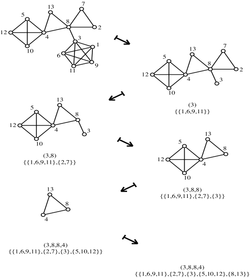
Figure 8: Prüfer correspondence for a Husimi graph

We now turn to the species of oriented cacti, defined in Example 1.1.6. These structures were introduced by Springer in [28] for the purpose of enumerating ”ordered short factorizations” of a circular permutation $\rho$ of length $n$ into circular permutations, $a_{i}$ of length $i$ for each $i$. Such a factorization is called short if $\sum_{i\geq 2}(i-1)a_{i}=n-1$.

Proposition 3.3

The number $\mathop{\rm Oc}\nolimits_{n}=|\mathop{\rm Oc}\nolimits[n]|$ of oriented cacti on $[n]$, for $n\geq 2$, is given by

$$\mathop{\rm Oc}\nolimits_{n}=\sum_{k\geq 1}\frac{(n-1)!}{k!}{n-2\choose k-1}\,n^{k-1},$$ (44)

where $k=\sum_{i\geq 2}n_{i}$ is the number of cycles.

Proof. The proof is similar to that of (39). Here $\mathcal{B}=\sum_{k\geq 2}C_{k}$, the species of oriented cycles of size $k\geq 2$ and $\mathcal{B}^{\prime}=\sum_{k\geq 1}X^{k}$, the species of ”lists” (totally ordered sets) of size $k\geq 1$. One can use Lagrange inversion formula, with $R(x)=\exp({x\over{1-x}})$. Alternately, observe that the factor $\frac{(n-1)!}{k!}{n-2\choose k-1}$ in (44) represents the number of partitions of a set of size $n-1$ into $k$ totally ordered parts so that the Prüfer-type bijection of Springer [28] can be used here. $\Box$

Proposition 3.4

[28] Let $(n_{2},n_{3},\ldots)$ be a sequence of non-negative integers and $n=\sum_{i\geq 2}n_{i}(i-1)+1$. Then the number $\mathop{\rm Oc}\nolimits(n_{2},n_{3},\ldots)$ of oriented cacti on $[n]$ having $n_{i}$ cycles of size $i$ for each $i$, is given by

$$\mathop{\rm Oc}\nolimits(n_{2},n_{3},\cdots)=\frac{(n-1)!}{n_{2}!n_{3}!\cdots}\,n^{k-1},$$ (45)

where $k=\sum_{i\geq 2}n_{i}$ is the number of cycles.

Proof. Again, it is possible to use Lagrange inversion or the Prüfer-type correspondence of Springer. However the result now follows simply from equation (42) since it is easy to see that

$$\mathop{\rm Oc}\nolimits(n_{2},n_{3},\ldots)=\prod_{i\geq 2}(i-1)!^{n_{i}}\mathop{\rm Hu}\nolimits(n_{2},n_{3},\ldots).$$

Indeed, a set of size $i$ can be structured into an oriented cycle in $(i-1)!$ ways. $\Box$

Finally, let us consider the species $\mathop{\rm Ca}\nolimits$ of cacti which is of the form $C_{\mathcal{B}}$, where $B=\sum_{k\geq 2}P_{k}$ is the species of polygons. By convention, a polygon of size $2$ is simply an edge ($K_{2}=E_{2}$). See Example 1.1.3 and Figure 3. These structures frequently appear in mathematical research, for example, more recently, in the context of the Traveling Salesman Problem (see for instance [4]) and in the classification of graphic matroids [Za02].

Proposition 3.5

(Ford and Uhlenbeck [5]) Let $(n_{2},n_{3},\ldots)$ be a sequence of non-negative integers and $n=\sum_{i\geq 2}n_{i}(i-1)+1$. Then the number $\mathop{\rm Ca}\nolimits(n_{2},n_{3},\ldots)$ of cacti on $[n]$ having $n_{i}$ polygons of size $i$ for each $i$, is given by

$$\mathop{\rm Ca}\nolimits(n_{2},n_{3},\cdots)=\frac{1}{2^{\sum_{j\geq 3}n_{j}}}\frac{(n-1)!}{\prod_{j\geq 2}n_{j}!}\,n^{k-1},$$ (46)

where $k=\sum_{i\geq 2}n_{i}$ is the number of polygons.

Proof. Indeed, since any (labelled) polygon of size $\geq 3$ has $2$ orientations, we see that

$$\mathop{\rm Oc}\nolimits(n_{2},n_{3}\ldots)=2^{\sum_{j\geq 3}n_{j}}\mathop{\rm Ca}\nolimits(n_{2},n_{3},\cdots).$$

The result then follows from (45). $\Box$

As observed in [5], this corrects the formula given in the introduction of [11] which is rather Husimi’s formula (42) for Husimi graphs. By summing over the polygon-size distribution, we finally obtain:

Proposition 3.6

The number $\mathop{\rm Ca}\nolimits_{n}=|\mathop{\rm Ca}\nolimits[n]|$ of (labelled) cacti on $[n]$, for $n\geq 2$, is given by

$$\mathop{\rm Ca}\nolimits_{n}=\sum_{k\geq 0}\sum_{{n_{2}+n_{3}+\cdots=k\atop n_{2}+2n_{3}+\cdots=n-1}}\frac{(n-1)!\ n^{k-1}}{2^{n_{3}+n_{4}+\cdots}\ n_{2}!n_{3}!\cdots}\ .$$ (47)

3.2 Unlabelled enumeration

For unlabelled enumeration, the cases of rooted and of unrooted $C_{\mathcal{B}}$-graphs must be treated separately. There is a basic species relationship which permits the expression of the unrooted species in terms of the rooted ones. It plays the role of the classical Dissimilarity characteristic theorem for graphs (see [10]). Let $\mathcal{B}$ be a species of 2-connected graphs and $C_{\mathcal{B}}$, the associated species of $C_{\mathcal{B}}$-graphs, that is of connected graphs with blocks in $\mathcal{B}$. We introduce the following notations:

1. $C_{\mathcal{B}}^{\diamondsuit}$ is the species of $C_{\mathcal{B}}$-graphs with a distinguished block,

2. $C_{\mathcal{B}}^{\bullet\negthinspace\diamondsuit}$ is the species of $C_{\mathcal{B}}$-graphs with a distinguished vertex-rooted block.

Theorem 3.7

Dissymmetry Theorem for Graphs [18], [19], [2]. The species $C_{\mathcal{B}}$ of connected graphs whose blocks are in $\mathcal{B}$ and its associated rooted species are related by the following isomophism:

$$C_{\mathcal{B}}^{\bullet}+C_{\mathcal{B}}^{\diamondsuit}=C_{\mathcal{B}}+C_{\mathcal{B}}^{\bullet\negthinspace\diamondsuit}.$$ (48)

This identity can also be written as

$$C_{\mathcal{B}}^{\bullet}+\mathcal{B}(C_{\mathcal{B}}^{\bullet})=C_{\mathcal{B}}+C_{\mathcal{B}}^{\bullet}\cdot\mathcal{B}^{\prime}(C_{\mathcal{B}}^{\bullet}).$$ (49)

Proof. The proof of (48) is remarkably simple. It uses the concept of center of a $C_{\mathcal{B}}$-graph, which is defined as the center of the associated block-cutpoint tree (see Figure 2, c)). The center will necessarily be either a vertex (in fact an articulation point), or a block of the $C_{\mathcal{B}}$-graph. Now a structure $s$ belonging to the left-hand-side of (48) is a $C_{\mathcal{B}}$-graph which is rooted at either a vertex or a block (a cell). It can happen that the rooting is performed right at the center. This is canonically equivalent to doing nothing and is represented by the first term in the right-hand-side of (48). On the other hand, if the rooting is done at an off-center cell, a vertex or a block, then there is a unique incident cell of the other kind (a block for a vertex and vice-versa) which is located towards the center, thus defining a unique $C_{\mathcal{B}}^{\bullet\negthinspace\diamondsuit}$-structure. It is easily checked that this correspondence is bijective and independent of any labelling, giving the desired species isomorphism.

For (49), it suffices to verify the species isomophisms $C_{\mathcal{B}}^{\diamondsuit}=\mathcal{B}(C_{\mathcal{B}}^{\bullet})$ and $C_{\mathcal{B}}^{\bullet\negthinspace\diamondsuit}=C_{\mathcal{B}}^{\bullet}\cdot\mathcal{B}^{\prime}(C_{\mathcal{B}}^{\bullet})$. Details are left as an exercise. $\Box$

The method of enumeration of unlabelled $C_{\mathcal{B}}$-graphs then consists in enumerating first the rooted unlabelled $C_{\mathcal{B}}$-graphs, using the functional equation (8) or (12), and then the unrooted ones, using (49). Notice that these steps will lead not to explicit but rather to recursive formulas for the desired numbers or total weights. Here we illustrate the method in detail in the case of triangular cacti (Example 1.1.4). We will also give some results for Husimi graphs and oriented cacti.

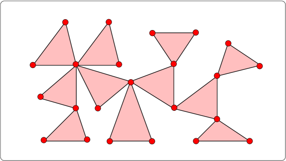
Figure 9: Unlabelled triangular cactus

Recall that a triangular cactus is a connected graph all of whose blocks are triangles. See Figure 9 for an example. These structures (and also the quadrangular cacti) were enumerated by Harary, Norman, and Uhlenbeck [9], [11]. Here we go further by giving recurrence formulas for their numbers. Let $\delta=C_{\mathcal{B}}$ and $\Delta=\delta^{\bullet}$ denote the species of triangular cacti and of rooted triangular cacti, respectively. Also set

$$\widetilde{\delta}(x)=\sum_{n\geq 1}d_{n}x^{n}\ \ \mathop{\rm and}\ \ \widetilde{\Delta}(x)=\sum_{n\geq 1}D_{n}x^{n},$$ (50)

where $d_{n}$ and $D_{n}$ denote the numbers of unlabelled triangular cacti and rooted triangular cacti, respectively. Here we have $\mathcal{B}=K_{3}=E_{3}$, and $\mathcal{B}^{\prime}=E_{2}$. The functional equations (8) and (49) give

$$\Delta=X\,E(E_{2}(\Delta))$$ (51)

and

$$\Delta+E_{3}(\Delta)=\delta+\Delta\,E_{2}(\Delta),$$ (52)

respectively. Note that

$$Z_{E\circ E_{2}}(x_{1},x_{2},x_{3},\ldots) = Z_{E}(Z_{E_{2}}(x_{1},x_{2},\ldots),Z_{E_{2}}(x_{2},x_{4},\ldots),\ldots)$$

$$= Z_{E}(\frac{1}{2}(x_{1}^{2}+x_{2}),\frac{1}{2}(x_{2}^{2}+x_{4}),\ldots)$$

$$= \exp{\left(\sum_{k\geq 1}\frac{1}{k}\frac{(x_{k}^{2}+x_{2k})}{2}\right)}.$$

From (51), we deduce (see [11])

$$\widetilde{\Delta}(x) = (XE(E_{2}(\Delta)))^{\sim}(x)$$ (53)

$$= xZ_{E\circ E_{2}}(\widetilde{\Delta}(x),\widetilde{\Delta}(x^{2}),\widetilde{\Delta}(x^{3}),\ldots)$$

$$= x\exp{\left(\sum_{k\geq 1}\frac{1}{2k}\left(\widetilde{\Delta}^{2}(x^{k})+\widetilde{\Delta}(x^{2k})\right)\right)}.$$

A recurrence formula for $D_{n}$ can be obtained by taking $x$ $\times$ the derivative of (53). First set

$$b(x)=x\frac{d}{dx}\sum_{k\geq 1}\frac{1}{2k}\left(\widetilde{\Delta}^{2}(x^{k})+\widetilde{\Delta}(x^{2k})\right).$$

We then have $x\widetilde{\Delta}^{\prime}(x)=\widetilde{\Delta}(x)+\widetilde{\Delta}(x)b(x)$ and

$$x\widetilde{\Delta}^{\prime}(x)-\widetilde{\Delta}(x)=\widetilde{\Delta}(x)b(x).$$ (54)

But

$$b(x) = x\frac{d}{dx}\sum_{k\geq 1}\frac{1}{2k}\left(\widetilde{\Delta}^{2}(x^{k})+\widetilde{\Delta}(x^{2k})\right)$$

$$= x\cdot\sum_{k\geq 1}\frac{1}{2k}\left(2\widetilde{\Delta}(x^{k})\widetilde{\Delta}^{\prime}(x^{k})kx^{k-1}+\widetilde{\Delta}^{\prime}(x^{2k})2kx^{2k-1}\right)$$

$$= \sum_{k\geq 1}\left(\widetilde{\Delta}(x^{k})\widetilde{\Delta}^{\prime}(x^{k})x^{k}+\widetilde{\Delta}^{\prime}(x^{2k})x^{2k}\right)$$

$$= \sum_{k\geq 1}\left(\sum_{h\geq 1}\sum_{j\geq 1}jD_{h}D_{j}x^{k(h+j)}+\sum_{j\geq 1}jD_{j}x^{2kj}\right)$$

$$= \sum_{m\geq 1}\left(\sum_{{d|m\atop d\geq 2}}\sum_{j=1}^{d}jD_{d-j}D_{j}+\sum_{{d|m\atop d\ \mbox{\tiny{even}}}}\frac{d}{2}D_{\frac{d}{2}}\right)x^{m}.$$

By extracting the coefficient of $x^{n+1}$ in (54), we obtain

Proposition 3.8

The numbers $D_{n}$, of unlabelled rooted triagular cacti on $n$ vertices satisfy $D_{1}=1$ and the recurrence formula, for $n\geq 1$,

$$D_{n+1}=\frac{1}{n}\sum_{m=1}^{n}D_{n-m+1}\left(\sum_{d|m\atop d\geq 2}\sum_{j=1}^{d}jD_{d-j}D_{j}+\sum_{{d|m\atop d\ \mbox{\tiny{even}}}}\frac{d}{2}D_{\frac{d}{2}}\right).$$ (55)

In order to enumerate unlabelled unrooted triangular cacti, we use (49), that is,

$$\delta=\Delta+E_{3}(\Delta)-\Delta E_{2}(\Delta).$$

The passage to the tilde generating functions yields (see [9])

$$\widetilde{\delta}(x) = \widetilde{\Delta}(x)+(E_{3}(\Delta(x)))^{\sim}-\widetilde{\Delta}(x)(E_{2}(\Delta(x)))^{\sim}$$ (56)

$$= \widetilde{\Delta}(x)+Z_{E_{3}}(\widetilde{\Delta}(x),\widetilde{\Delta}(x^{2}),\ldots)-\widetilde{\Delta}(x)Z_{E_{2}}(\widetilde{\Delta}(x),\widetilde{\Delta}(x^{2}),\ldots)$$

$$= \widetilde{\Delta}(x)+\frac{1}{6}(\widetilde{\Delta}^{3}(x)+3\widetilde{\Delta}(x)\widetilde{\Delta}(x^{2})+2\widetilde{\Delta}(x^{3}))-\frac{1}{2}\widetilde{\Delta}(x)(\widetilde{\Delta}^{2}(x)+\widetilde{\Delta}(x^{2}))$$

$$= \widetilde{\Delta}(x)+\frac{1}{3}\left(\widetilde{\Delta}(x^{3})-\widetilde{\Delta}^{3}(x)\right).$$

By extracting the coefficient of $x^{n}$, we finally obtain

Proposition 3.9

The numbers $d_{n}$, of unlabelled (unrooted) triangular cacti on $n$ vertices satisfy, for $n\geq 1$,

$$d_{n}=D_{n}+\frac{1}{3}\left(\mbox{\Large{$\chi$}}(3|n)D_{\frac{n}{3}}-\sum_{i+j+k=n}D_{i}D_{j}D_{k}\right).$$ (57)

We now turn our attention to the species $\mathop{\rm Hu}\nolimits$ of Husimi graphs. Let us denote by $h_{n}$ and $H_{n}$, the numbers of unlabelled Husimi graphs and rooted Husimi graphs, respectively, and set

$$h(x)=\sum_{n\geq 1}h_{n}x^{n}=\widetilde{\mathop{\rm Hu}\nolimits}(x)\ \ \mathop{\rm and}\ \ H(x)=\sum_{n\geq 1}H_{n}x^{n}=\widetilde{\mathop{\rm Hu}\nolimits^{\bullet}}(x).$$ (58)

Here, as seen in Section 3.1, $\mathcal{B}=E_{\geq 2}$ and $\mathcal{B}^{\prime}=E_{\geq 1}=E_{+}$, and the basic functional equation (40) translates, for the tilde generating function, into (see [24], p. 51)

$$H(x)=x\exp{\sum_{k\geq 1}\frac{1}{k}\left(\exp{\left(\sum_{m\geq 1}\frac{1}{m}H(x^{mk})\right)-1}\right)}.$$ (59)

We introduce the auxiliary series

$$b(x)=\sum_{n\geq 1}b_{n}x^{n}=x\frac{d}{dx}\sum_{k\geq 1}\frac{1}{k}\left(\exp\left(\sum_{m\geq 1}\frac{1}{m}H(x^{mk})\right)-1\right),$$ (60)

$$\varphi(x)=\sum_{n\geq 1}\varphi_{n}x^{n}=x\exp{\left(\sum_{j\geq 1}\frac{1}{j}\mathop{\rm H}\nolimits(x^{j})\right)}.$$ (61)

Then, after some computations, similar to those for triangular cacti, we find:

Proposition 3.10

The numbers $H_{n}$, of unlabelled rooted Husimi graphs on $n$ vertices can be computed by the following recusive scheme:   $\varphi_{1}=1$,   $H_{1}=1$,   and, for $n\geq 1$,

$$b_{n} = \sum_{d|n}\sum_{h=1}^{d}\sum_{l|d-h+1}lH_{l}\ \varphi_{h},$$ (62)

$$H_{n+1} = \frac{1}{n}\sum_{k=1}^{n}H_{n-k+1}b_{k},$$ (63)

$$\varphi_{n+1} = \frac{1}{n}\sum_{m=1}^{n}\varphi_{n-m+1}\sum_{d|m}dH_{d}.$$ (64)

For unlabelled unrooted Husimi graphs, we use the Dissymmetry Theorem, in the form (49), which gives

$$\mathop{\rm Hu}\nolimits^{\bullet}+E_{\geq 2}(\mathop{\rm Hu}\nolimits^{\bullet}) = \mathop{\rm Hu}\nolimits+\mathop{\rm Hu}\nolimits^{\bullet}\cdot E_{+}(\mathop{\rm Hu}\nolimits^{\bullet}),$$

$$E_{+}(\mathop{\rm Hu}\nolimits^{\bullet}) = \mathop{\rm Hu}\nolimits+\mathop{\rm Hu}\nolimits^{\bullet}\cdot E_{+}(\mathop{\rm Hu}\nolimits^{\bullet}),$$

and finally

$$\mathop{\rm Hu}\nolimits=(E_{+}(\mathop{\rm Hu}\nolimits^{\bullet}))\cdot(1-\mathop{\rm Hu}\nolimits^{\bullet}).$$ (65)

For the tilde generating series, we deduce that

$$h(x) = \left(\exp{\left(\sum_{k\geq 1}\frac{1}{k}H(x^{k})\right)}-1\right)\cdot\left(1-H(x)\right)$$

$$= \left(\frac{\varphi(x)}{x}-1\right)\cdot\left(1-H(x)\right),$$

and we obtain the following result.

Proposition 3.11

The numbers $h_{n}$, of unlabelled Husimi graphs on $n$ vertices satisfy

$$h_{n}=\varphi_{n+1}-\sum_{k=1}^{n-1}\varphi_{k+1}H_{n-k},$$ (66)

where the numbers $H_{n}$ and $\varphi_{n}$ are given by Proposition 3.10.

The same method can be applied to weighted $C_{\mathcal{B}}$-graphs where the weight is defined by (11), that is, with the variables $(y_{2},y_{3},\ldots)$ marking the block sizes. We have done the computations for the weighted species $\mathop{\rm Oc}\nolimits_{w}$, of oriented cacti, where $\mathcal{B}_{w}=\sum_{m\geq 2}(C_{m})_{y_{m}}$ and $\mathcal{B}^{\prime}_{w}=\sum_{m\geq 1}(L_{m})_{y_{m+1}}$, where $(C_{m})_{y_{m}}$ denotes the species of oriented cycles of length $m$ and weight $y_{m}$, and $L_{m}=X^{m}$ is the species of lists of size $m$, endowed here with the weight $y_{m+1}$. Introduce the following tilde generating series, whose coefficients are polynomials in the variables $\textbf{y}=(y_{2},y_{3},\ldots)$:

$$o(x;\textbf{y}):=\widetilde{\mathop{\rm Oc}\nolimits_{w}}(x) = \sum_{n\geq 1}o_{n}({\textbf{y}})x^{n},$$

$$O(x;\textbf{y}):=\widetilde{\mathop{\rm Oc}^{\bullet}\nolimits_{w}}(x) = \sum_{n\geq 1}O_{n}({\textbf{y}})x^{n}.$$

The two basic species functional equations are

$$\mathop{\rm Oc}^{\bullet}\nolimits_{w}=X\cdot E\left(\sum_{m\geq 1}(L_{m})_{y_{m+1}}(\mathop{\rm Oc}^{\bullet}\nolimits_{w})\right),$$ (67)

$$C_{w}(\mathop{\rm Oc}^{\bullet}\nolimits)=\mathop{\rm Oc}\nolimits+L_{\geq 2,w}(\mathop{\rm Oc}^{\bullet}\nolimits),$$ (68)

where $C_{w}=\sum_{m\geq 1}(C_{m})_{y_{m}}$, with $C_{1}=X,\ y_{1}=1$, and $L_{\geq 2,w}=\sum_{m\geq 2}(X^{m})_{y_{m}}$. Note that

$$Z_{C_{w}}=\sum_{m\geq 1}\frac{y_{m}}{m}\sum_{d|m}\phi(d)x_{d}^{\frac{m}{d}}=\sum_{d\geq 1}\sum_{h\geq 1}\frac{y_{dh}}{dh}\phi(d)x_{d}^{h},$$

where $\phi$ is Euler’s totient function, and that $Z_{L_{\geq 2,w}}=\sum_{m\geq 2}y_{m}x_{1}^{m}$. From (67), we deduce, using the plethystic composition rule for the tilde generating function of weighted species (see (4.3.1) of [2]),

$$O(x;\textbf{y})=x\exp{\left(\sum_{k\geq 1}\frac{1}{k}\sum_{j\geq 1}y_{j+1}^{k}O^{j}(x^{k};\textbf{y}^{k})\right)},$$ (69)

where $\textbf{y}^{k}=(y_{2}^{k},y_{3}^{k},\ldots)$. We then set

$$O^{j}(x;\textbf{y})=(O(x;\textbf{y}))^{j}=\sum_{n\geq 1}O_{n}^{(j)}({\textbf{y}})x^{n},$$ (70)

$$b(x;\textbf{y})=\sum_{m\geq 1}b_{m}(\textbf{y})x^{m}=x\frac{\partial}{\partial x}\sum_{k\geq 1}\frac{1}{k}\sum_{j\geq 1}y_{j+1}^{k}O^{j}(x^{k};\textbf{y}^{k}).$$ (71)

From (68), we deduce

$$o(x;\textbf{y})=\sum_{d\geq 1}\phi(d)\sum_{h\geq 1}\frac{y_{dh}}{dh}O(x^{d};\textbf{y}^{d})-\sum_{m\geq 2}y_{m}O(x;\textbf{y})^{m}$$ (72)

and we obtain, after some computations, the following result.

Proposition 3.12

The generating polynomials $O_{n}(\textbf{y})$ and $o_{n}(\textbf{y})$ for unlabelled rooted and unrooted (resp.) oriented cacti on $n$ vertices are given by the following recursive scheme:

$$O_{n+1}(\textbf{y})=\frac{1}{n}\sum_{m=1}^{n}O_{n-m+1}(\textbf{y})b_{m}(\textbf{y}),$$ (73)

where

$$b_{m}(\textbf{y})=\sum_{d|m}\sum_{i=1}^{d}\sum_{j=1}^{d-i+1}ij\ y_{j+1}^{\frac{m}{d}}O_{i}(\textbf{y}^{\frac{m}{d}})O_{d-i}^{(j-1)}(\textbf{y}^{\frac{m}{d}}),$$ (74)

and

$$o_{n}(\textbf{y})=\sum_{d|n}\phi(d)\sum_{h=1}^{\frac{n}{d}}\frac{y_{dh}}{dh}O_{\frac{n}{d}}^{(h)}(\textbf{y}^{d})-\sum_{m=2}^{n}y_{m}O_{n}^{(m)}(\textbf{y}).$$ (75)

4 Molecular expansions

The molecular expansion of a species $F$ is a description and a classification of the unlabelled $F$-structures according to their stabilizers, within the language of species. It is interesting and useful to have at hand the first few terms of the molecular expansion of $C_{\mathcal{B}}$-graphs. This is possible with the Maple package Devmol, developped at LaCIM. See [1].

As an example, consider again the species $\mathop{\rm Hu}\nolimits_{w}$ of Husimi graphs, weighted according to their block-size distribution. Here $\mathcal{B}_{w}=E_{\geq 2,w}=\sum_{k\geq 2}(E_{k})_{y_{k}}$. This is the species $BB$ in the following extract from a Maple session, using the package Devmol. The Devmol procedure ”CBgraphes(BB,n)” produces the molecular expansion of the species of $\mathcal{C}_{BB}$-graphs, up to the given truncation order $n$. The expansion is then collected by degree (vertex number). The weight variables $y_{2},y_{3},\ldots,y_{n}$ are first declared to Devmol. Afterwards, the monomial weights in the $y_{i}$’s appear multiplicatively in the expressions. Here is the extract:

$>$    n := 6;

$$n:=6$$

$>$    ajoutvv(seq(y[k], k = 1..n));

$$\{t,\,{y_{1}},\,{y_{2}},\,{y_{3}},\,{y_{4}},\,{y_{5}},\,{y_{6}}\}$$

$>$    BB := sum(y[k]*E[k](X), k = 2..n);

$$\begin{array}[]{c}BB:={y_{2}}\,{E_{2}}(X)+{y_{3}}\,{E_{3}}(X)+{y_{4}}\,{E_{4}}(X)+{y_{5}}\,{E_{5}}(X)+{y_{6}}\,{E_{6}}(X)\end{array}$$

$>$    HuW := CBgraphes(BB,n):

$>$    affichertable(tablephom(HuW));

$$\begin{array}[]{c}1\\ X\end{array}$$

$$\begin{array}[]{c}2\\ {y_{2}}\,{E_{2}}(X)\end{array}$$

$$\begin{array}[]{c}3\\ X\,{y_{2}}^{2}\,{E_{2}}(X)+{y_{3}}\,{E_{3}}(X)\end{array}$$

$$\begin{array}[]{c}4\\ {y_{2}}\,X^{2}\,{y_{3}}\,{E_{2}}(X)+X\,{y_{2}}^{3}\,{E_{3}}(X)+{y_{2}}^{3}\,{E_{2}}(X^{2})+{y_{4}}\,{E_{4}}(X)\end{array}$$

$$\begin{array}[]{c}5\\ ({y_{3}}\,{y_{2}}^{2}+{y_{2}}^{4})\,X^{3}\,{E_{2}}(X)+X\,{y_{2}}^{2}\,{E_{2}}(X)^{2}\,{y_{3}}+({y_{3}}\,{y_{2}}^{2}+{y_{2}}^{4})\,X\,{E_{2}}(X^{2})\\ +X\,{y_{2}}^{4}\,{E_{4}}(X)+X\,{y_{3}}^{2}\,{E_{2}}({E_{2}}(X))+{y_{5}}\,{E_{5}}(X)+{y_{2}}\,X^{2}\,{y_{4}}\,{E_{3}}(X)\par\end{array}$$

$$\begin{array}[]{c}6\\ {y_{2}}^{5}\,X^{2}\,{E_{2}}(X^{2})+({y_{2}}^{2}\,{y_{4}}+{y_{3}}\,{y_{4}}+{y_{3}}\,{y_{2}}^{3})\,X\,{E_{2}}(X)\,{E_{3}}(X)\\ +{y_{4}}\,{E_{2}}(X)\,{y_{2}}^{2}\,{E_{2}}(X^{2})\mbox{}+({y_{3}}^{2}\,{y_{2}}+{y_{2}}^{5}+3\,{y_{3}}\,{y_{2}}^{3})\,X^{4}\,{E_{2}}(X)\\ +{y_{2}}^{5}\,{E_{2}}(X^{3})+({y_{3}}^{2}\,{y_{2}}+{y_{2}}^{5})\,{E_{2}}(X\,{E_{2}}(X))\mbox{}+{y_{2}}\,{y_{3}}^{2}\,X^{2}\,{E_{2}}({E_{2}}(X))\\ +{y_{3}}\,{y_{2}}^{3}\,{E_{3}}(X^{2})+{y_{2}}\,{y_{5}}\,X^{2}\,{E_{4}}(X)+{y_{6}}\,{E_{6}}(X)+{y_{3}}\,{y_{2}}^{3}\,X^{2}\,{E_{2}}(X)^{2}\\ \mbox{}+{y_{3}}\,{y_{2}}^{3}\,X^{6}+({y_{2}}^{5}+{y_{2}}^{2}\,{y_{4}})\,X^{3}\,{E_{3}}(X)+{y_{2}}^{5}\,X\,{E_{5}}(X)\end{array}$$

Figure 10: Husimi graphs of size $5$

As an illustration, the nine terms of size $5$ are shown in Figure 10. Observe that multiciplicities will frequently occur in these expansions. For size $6$, for example, the term $3\,y_{3}\,y_{2}^{3}\,X^{4}E_{2}(X)$ corresponds to the $3$ similar types of Husimi graphs shown in Figure 11.

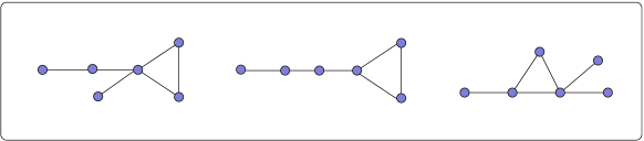
Figure 11: The three unlabelled Husimi graphs of molecular type $y_{2}^{3}y_{3}\cdot X^{4}E_{2}(X)$

Pierre Leroux
LaCIM, Dép. de mathématiques,
Université du Québec à Montréal,
C.P. 8888, Succ. Centre-Ville,
Montréal (Québec), Canada H3C 3P8.
leroux.pierre@uqam.ca, www.lacim.uqam.ca/$\sim$leroux

References

-
[1]
Pierre Auger, Pierre Leroux and Gilbert Labelle, Computing the molecular expansion of species
with the Maple Package Devmol, Séminaire Lotharingien de Combinatoire, 2002, B49z (2003), 34 pp.
http://igd.univ-lyon1.fr/ webeuler/home/slc/wpapers/s49leroux.html - [2] François Bergeron, Gilbert Labelle and Pierre Leroux. Combinatorial Species and Tree-Like Structures, Coll. Encyclopedia of mathematics and its applications, Vol. 67, Cambridge University Press, 1998, 457 p.
- [3] Miklós Bóna, Michel Bousquet, Gilbert Labelle and Pierre Leroux, Enumeration of -ary cacti, Advances in Applied Mathematics, 24, 2000, 22–56.
- [4] Lisa Fleischer, Building chain and cactus representations of all minimum cuts from Hao-Orlin in the same asymptotic run time, J. Algorithms, 33, 1999, 51–72.
- [5] George Ford and George Uhlenbeck, Combinatorial Problems in the Theory of Graphs, I, Proc. Nat. Acad. Sciences, 42 (1956), 122–128.
- [6] George Ford, Robert Norman and George Uhlenbeck, Combinatorial Problems in the Theory of Graphs, II, Proc. Nat. Acad. Sciences, 42 (1956), 203–208.
- [7] Tom Fowler, Ira Gessel, Gilbert Labelle and Pierre Leroux, The specification of 2-tress, Advances in Applied Mathematics, 28, 2002, 145–168.
- [8] Frank Harary, Graph Theory, Addison-Wesley, 1969, 274 p.
- [9] Frank Harary and Robert Norman. The dissimilarity characteristic of Husimi trees, Ann. of Math., 58, 1953, 134–141.
- [10] Frank Harary and Edgar Palmer. Graphical Enumeration, Academic Press, New York and London, 1973, 271 p.
- [11] Frank Harary and George Uhlenbeck. On the number of Husimi trees, Proc. Nat. Aca. Sci., 39, 1953, 315–322.
- [12] Kodi Husimi. Note on Mayers’ theory of cluster integrals, The Journal of Chemical Physics, 18, 1950, 682–684.
- [13] André Joyal, Une théorie combinatoire des séries formelles, Advances in Mathematics, 42, 1981, 1–82.
- [14] Gilbert Labelle, Counting asymmetric enriched trees, Journal of Symbolic Computation, 14, 1992, 211–242.
- [15] G. Labelle, C. Lamathe, P. Leroux, Énumération des 2-arbres -gonaux, Proceedings of the conference Mathematics and Computer Science: Algorithms, Trees, Combinatorics and Probabilities, Versailles, September 16–19, 2002, in Mathematics and Computer Science II, B. Chauvin, P. Flajolet, D. Gardy, and A. Mokkadem, ed., Birkhäuser, Basel, 2002, 95–109.
- [16] Gilbert Labelle, Cédric Lamathe and Pierre Leroux, A classification of plane and planar 2-trees, Theoretical Computer Science, 307 (2003), 337–363.
- [17] Labelle, Jacques, Applications diverses de la théorie combinatoire des espèces de structures, Annales des Sciences Mathématiques du Québec, 7, 1983, 59–94.
- [18] Pierre Leroux, Methoden der Anzahlbestimmung für einige Klassen von Graphen, Bayreuther Mathematische Schriften, 26, 1988, 1–36.
- [19] Pierre Leroux and Brahim Miloudi Généralisations de la formule d’Otter, Annales des Sciences Mathématiques du Québec, 16, 1992, 53–80.
- [20] F. Maffioli and N. Zagaglia Salvi, A characterization of the base-matroids of a graphic matroid, Preprint, 2003.
- [21] J. E. Mayer and M. G. Mayer, Statistical Mechanics, Wiley, New York, 1940.
- [22] J. E. Mayer, Equilibrium Statistical Mechanics, The international encyclopedia of physical chemistry and chemical physics, Pergamon Press, Oxford, 1968, 242 p.
- [23] Mélanie Nadeau, Graphes de Husimi, Cactus, et mécanique statistique. Mémoire de maîtrise, UQAM, 2002.
- [24] R. Z. Norman, On the number of linear graphs with given blocks, Dissertation, University of Michigan, 1954.
- [25] Richard Otter, The number of trees, Ann. of Math, 49, 1948, 583–599.
- [26] Robert Riddell . Contributions to the theory of condensation, Dissertation, University of Michigan, Ann Arbor, 1951.
- [27] Robert Robinson Enumeration of non-separable graphs, Journal of Combinatorial Theory, 9, 1970, 327–356.
- [28] Colin Springer, Factorizations, Trees, and Cacti, Proceedings of the Eighth International Conference on Formal Power Series and Algebraic Combinatorics (FPSAC), University of Minnesota, 1996, 427–438.
- [29] George Uhlenbeck et George Ford, Lectures in Statistical Mechanics, Amer. Math. Soc., Providence, Rhode Island, 1963, 181 p.