The Denjoy type-of argument for quasiperiodically forced circle diffeomorphisms

Abstract

We carry the argument used in the proof of the Theorem of Denjoy over to the quasiperiodically forced case. Thus we derive that if a system of quasiperiodically forced circle diffeomorphisms with bounded variation of the derivative has no invariant graphs with a certain kind of topological regularity, then the system is topologically transitive.

1 Introduction

When studying quasiperiodically forced circe maps, it is an obvious question to ask to what extent the results for unperturbed circle homeomorphisms and diffeomorphisms carry over. Invariant graphs serve as a natural analogue for fixed or periodic points. Unfortunately, a system without invariant graphs is not necessarily conjugated to an irrational torus translation (at least not if the conjugacy is required to respect the skew product structure; a simple counterexample will be given in Section 2). However, there is a result by Furstenberg ([Fur61]), which may be considered as an anologue to the Poincaré classification for circle homeomorphisms in a measure-theoretic sense: It states that for a system of quasiperiodically forced circle maps either there exists an invariant graph, then all invariant ergodic measures are associated to invariant graphs, or the system is uniquely ergodic with respect to an invariant measure which is continuous on the fibres. In the latter case the system will be isomorphic to a skew translation of the torus by an isomorphism with some additional nice properties. We will briefly discuss Furstenbergs results after we have introduced the concept of invariant graphs in Section 2.

The (fibrewise) rotation number can be defined in the same way as the rotation number of a circle homeomorphism, but Herman already gave examples where invariant graphs exist in combination with arbitrary rotation numbers (see [Her83]). Thus the connection between the existence of fixed or periodic points and rational rotation numbers seems to break down in the forced case. However, this is different if we require a certain amount of topological regularity of the invariant graphs, in particular when the invariant graphs are continuous. Then the structure of an invariant graph already determines the fibrewise rotation number, and this is described in Section 3. It might be considered well-known folklore, but as we knew of no apropriate reference and need a slight generalization afterwards it seemed apropriate to include some details.

Section 4 contains our main result, namely Theorem 4.4. ${\cal T}_{\textrm{BV}}$ denotes the class of systems where the variation of the logarithm of the derivative of the fibre maps is integrable. The concept of a regular $p,q$-invariant graph and its implications for the rotation numbers are introduced in Sections 2 and 3, as mentioned. The statement we derive then reads as follows: :

If $T\in{\cal T}_{\textrm{BV}}$ is not topologically transitive, then there exists a regular $p,q$-invariant graph for $T$. In particular, $\rho_{T}$ depends rationally on $\omega$, i.e. $\rho_{T}=\frac{k}{q}\omega+\frac{l}{pq}\bmod 1$ for suitable integers $k$ and $l$.

The question whether such systems are minimal (as in the unforced case) has to be left open here. However, if there exists a minimal strict subset of the circle then some further conclusions about its structure can be drawn.

2 Invariant graphs and invariant measures

We study quasiperiodically forced circle homeomorphisms and diffeomorphisms, i.e. continuous maps of the form

$$T:\mathbb{T}^{2}\rightarrow\mathbb{T}^{2}\ ,\ (\theta,x)\mapsto(\theta+\omega,T_{\theta}(x))\ ,$$ (2.1)

where the fibre maps $T_{\theta}$ are either orientation-preserving circle homeomorphisms or orientation-preserving circle diffeomorphisms with the derivative $DT_{\theta}$ depending continuously on $(\theta,x)$. To ensure all required lifting properties we additionally assume that $T$ is homotopic to the identity on $\mathbb{T}^{2}$. The classes of such systems will be denoted by ${\cal T}_{\textrm{hom}}$ and ${\cal T}_{\textrm{diff}}$ respectively. In all of the following, $m$ will be the Lebesgue-measure on $\mathbb{T}^{1}$, $\lambda$ the Lebesgue-measure on $\mathbb{T}^{2}$ and $\pi_{i}:\mathbb{T}^{2}\rightarrow\mathbb{T}^{1}\ (i=1,2)$ the projection to the respective coordinate. When considering fibre maps of iterates of $T$ or their inverses, we use the convention $T_{\theta}^{n}:=(T^{n})_{\theta}\ \forall n\in\mathbb{Z}$. Finally, by $\mathbb{T}^{n}_{*}$ we denote the set of all points $(x_{1},\ldots,x_{n})\in\mathbb{T}^{n}$ with $x_{i}\neq x_{j}\ \forall i,j:1\leq i<j\leq n$.

Invariant graphs. Due to the aperiodicity of the forcing rotation, there cannot be any fixed or periodic points for a system of the form (2.1). The simplest invariant objects will therefore be invariant graphs. In contrast to quasiperiodically forced monotone interval maps, where such invariant graphs are always one-valued functions, these might be multi-valued when circle maps are considered and the definition therefore needs a little bit more care. We will usually not distinguish between invariant graphs as functions and as point sets. This might seem a bit confusing at some times, but it is very convenient at others.

Definition 2.1 ($p,q$-invariant graphs)

Let $T\in{\cal T}_{\textrm{hom}}$, $p,q\in\mathbb{N}$. A $p,q$-invariant graph is a measurable function $\varphi:\mathbb{T}^{1}\rightarrow\mathbb{T}^{pq}_{*}\ ,\ \theta\mapsto\displaystyle(\varphi^{i}_{j}(\theta))^{\scriptscriptstyle 1\leq i\leq p}_{\scriptscriptstyle 1\leq j\leq q}$ with

$$T_{\theta}(\{\varphi_{1}^{1}(\theta),\ldots,\varphi^{p}_{q}(\theta)\})\ =\ \{\varphi_{1}^{1}(\theta+\omega),\ldots,\varphi^{p}_{q}(\theta+\omega)\}$$ (2.2)

for $m$-a.e. $\theta\in\mathbb{T}^{1}$, which satisfies the following:

• $\varphi$ cannot be decomposed (in a measurable way) into disjoint subgraphs $\varphi^{1},\ldots,\varphi^{m}\ (m\in\mathbb{N})$ which also satisfy (2.2).

• $\varphi$ can be decomposed into $p$ $p$-periodic $q$-valued subgraphs $\varphi^{1},\ldots,\varphi^{p}$.

• The subgraphs $\varphi^{1},\ldots,\varphi^{p}$ cannot further be decomposed into invariant or periodic subgraphs.

If $p=q=1$, $\varphi$ is called a simple invariant graph. The point set $\Phi:=\{(\theta,\varphi^{i}_{j}(\theta))\mid\theta\in\mathbb{T}^{1},\ 1\leq i\leq p,\ 1\leq j\leq q\}$ will also be called an invariant graph, but labeled with the corresponding capital letter. An invariant graph is called continuous if it is continuous as a function $\mathbb{T}^{1}\rightarrow\mathbb{T}^{pq}_{*}$.

Note that by this convention an invariant graph is a minimal object in the sense that it is not decomposable into smaller invariant parts. Therefore, the union of two or more invariant graphs will not be called an invariant graph again. On the other hand, it is always possible to decompose an invariant set which is the graph of a $n$-valued function into the disjoint union of invariant graphs:

Lemma 2.2

Let $T\in{\cal T}_{\textrm{hom}}$ and suppose $F:\mathbb{T}^{1}\rightarrow\mathbb{T}^{n}$ satisfies

$$T_{\theta}(\{F_{1}(\theta),\ldots,F_{n}(\theta)\})\ =\ \{F_{1}(\theta+\omega),\ldots,F_{n}(\theta+\omega)\}\ \ m\textrm{-a.s.\ .}$$

Then $\textrm{graph}(F)$ can be decomposed in exactly one way (modulo permutation) into $k$ disjoint $p,q$-invariant graphs $\Phi^{i}$, i.e. $\textrm{graph}(F)=\bigcup_{i=1}^{k}\Phi^{k}$, with $kpq=n$.

Proof.

Uniqueness: Any two invariant graphs are either disjoint or equal on $m$-a.e. fibre, otherwise their intersection would define an invariant subgraph. Thus if $\Psi^{1},\ldots,\Psi^{l}$ is another decomposition of $\textrm{graph}(F)$ into invariant graphs, then every $\Psi^{j}$ must be equal to some $\Phi^{i}$ (as it cannot be disjoint to all of them). This immediately implies the uniqueness of the decomposition.  
Existence: $\textrm{graph}(F)$ is either an invariant graph itself or can be decomposed into subgraphs which are invariant as point sets. The same is true for any such subgraph and after at most $n$ steps this yields an invariant graph $\hat{\varphi}$. This is either a $1,q$-periodic invariant graph, or it contains a periodic subgraph. Again, after a finite number of steps this yields some $p$-periodic graph $\varphi^{1}=\varphi_{1}^{1},\ldots,\varphi_{q}^{1}$ which is not further decomposable into invariant or periodic subgraphs. W.l.o.g. we can assume that the points $\varphi^{1}_{j}$ are ordered in $\mathbb{T}^{1}$, i.e. $\varphi^{1}_{1}(\theta)<\varphi^{1}_{2}(\theta)<\ldots<\varphi^{1}_{q}(\theta)<\varphi^{1}_{1}(\theta)$. Now for $m$-a.e. $\theta\in\mathbb{T}^{1}$ all the intervals $[\varphi^{1}_{i}(\theta),\varphi^{1}_{i+1}(\theta)]$ contain the same number of points $F_{j}(\theta)$, otherwise it would be possible to define an $T^{p}$-invariant subgraph of $\varphi^{1}$. Thus, by setting $\varphi_{i}^{l}(\theta):=$ $l$th point of $\{F_{1}(\theta),\ldots,F_{n}(\theta)\}$ in $[\varphi^{1}_{i}(\theta),\varphi^{1}_{i+1}(\theta)]$, the required decomposition of $\textrm{graph}(F)$ into $p,q$-invariant graphs can be defined.

∎

Of course, an example of a $p,1$-invariant graph can always be given by choosing a circle homeomorphism $f$ with a periodic point of period $p$ and taking $T_{\theta}=f\ \forall\theta\in\mathbb{T}^{1}$. Then the periodic orbit of $f$ defines a constant $p,1$-invariant graph. For $q\neq 1$ the situation is slightly more complicated, and there is no direct analogue for $1,q$-invariant graphs in the unperturbed case. The appropriate picture in this case is rather an invariant line for a flow on the torus, as the following example shows. The fact that invariant graphs may correspond to these two different types of dynamics, or both at once, will come up again later, namely in the proof of Thm. 4.4 .

Simple examples for $p,q$-invariant graphs with arbitrary $p$ and $q$ are given by torus translations: Consider $T:\mathbb{T}^{2}\rightarrow\mathbb{T}^{2},\ (\theta,x)\mapsto(\theta+\omega,x+\frac{k}{q}\omega+\frac{l}{pq})$ with $k$ relatively prime to $q$ and $l$ relatively prime to $p$. Then

$$\varphi^{i}_{j}(\theta):=\frac{k}{q}\theta+\frac{i-1+(j-1)p}{pq}\hskip 40.00006pt(1\leq i\leq p,\ 1\leq j\leq q)$$

defines a continuous $p,q$-invariant graph. The meaning of the numbers $k$ and $l$ will be explained in Section 3. Note that the motion on $\Phi^{i}$ induced by the action of $T^{p}$ is equivalent to an irrational rotation on $\mathbb{T}^{1}$ (by $\frac{p}{q}\omega+\frac{\tilde{l}}{q}$ where $l=\tilde{l}k\bmod q$), such that it is not possible to decompose these graphs into smaller invariant components.

Furstenberg’s results. As mentioned before, even in the absence of invariant graphs conjugacy to an irrational torus translation cannot be expected, at least not if we want the conjugacy to respect the skew product structure:

Example 2.3

A skew translation of the torus is a map $T:\mathbb{T}^{2}\rightarrow\mathbb{T}^{2},\ (\theta,x)\mapsto(\theta+\omega,x+g(\theta)\bmod 1)$ with some measurable function $g:\mathbb{T}^{1}\rightarrow\mathbb{R}$. When $g$ is continuous, a fibrewise rotation number $\rho_{T}$ can be assigned to $T$ (see Def. 3.1), and $\rho_{T}$ will be equal to $\tau:=\int_{\mathbb{T}^{1}}g(\theta)\ d\theta$. As conjugacy preserves the rotation numbers, $T$ can only be conjugated to the irrational torus translation $R:(\theta,x)\mapsto(\theta+\omega,x+\tau)$.

Now suppose $\tau\notin Q:=\{\frac{k}{q}\omega+\frac{l}{p}\bmod 1\mid k,q,l,p\in\mathbb{Z},\ p,q\neq 0\}$. Then $R$ is uniquely ergodic, and if $T$ and $R$ are conjugated (via a conjugacy $h$) so will be $T$. Thus $h$ must preserve the Lebesgue measure, which is invariant under both transformations. If we require the conjugacy to respect the skew product structure of the system, i.e. $\pi_{1}\circ h(\theta,x)=\theta\ \forall(\theta,x)\in\mathbb{T}^{2}$, then all fibre maps $h_{\theta}$ must also preserve Lebesgue measure and therefore be rotations. Hence $h$ will be a skew translation as well, i.e. $h(\theta,x)=(\theta,x+\varphi(\theta)\bmod 1)$ for some continuous function $\varphi:\mathbb{T}^{1}\rightarrow\mathbb{R}$. As $R=h^{-1}\circ T\circ h$ this function $\varphi$ is a continuous solution of the cohomology equation

$$g(\theta)-\tau=\varphi(\theta+\omega)-\varphi(\theta)\ .$$ (2.3)

Conversely, if a function $g$ has measurable, but no continuous solutions of (2.3), then on the one hand the resulting system $T$ cannot be conjugated to an irrational torus translation. On the other hand $T$ will still not have any invariant graphs, because a (non-continuous) solution $\varphi$ of (2.3) still allows to define an isomorphism $h$ between $T$ and $R$ as above. Thus $T$ will still be uniquely ergodic with respect to the Lebesgue measure on $\mathbb{T}^{2}$. An example of such a function $g$ is explicitly constructed in [KH97] (Section 12.6(b)).

This means that a possible analogue to the Poincaré classification for circle homeomorphisms must be somewhat weaker in nature. It turned out that the right perspective is to look at the invariant ergodic measures (see [Fur61]). First note that to any invariant graph an invariant ergodic measure can be assigned:

Definition 2.4 (Associated measure)

Let $\varphi$ be a $p,q$-invariant graph. Then

$$\mu_{\varphi}(A):=\frac{1}{pq}\sum_{i=1}^{p}\sum_{j=1}^{q}m(\{\theta\in\mathbb{T}^{1}:(\theta,\varphi^{i}_{j}(\theta))\in A\})\ \ \forall A\in{\cal B}(\mathbb{T}^{2})$$ (2.4)

defines an invariant ergodic measure. If $\mu=\mu_{\varphi}$ for some $p,q$-invariant graph $\varphi$, then $\mu$ and $\varphi$ are called associated to each other.

In order to study general invariant ergodic measures, it is useful to look at the so-called fibre measures. Any invariant measure $\mu$ can be disintegrated in the way $\mu=m\times K$ where $K$ is a stochastic kernel from $\mathbb{T}^{1}$ to $\mathbb{T}^{1}$, such that $\mu(A)=\int_{\mathbb{T}^{1}}K(\theta,A_{\theta})\ d\theta\ \forall A\in{\cal B}(\mathbb{T}^{2})$. The measures $\mu_{\theta}:=K(\theta,\textbf{.})$ on $\mathbb{T}^{1}$ are the fibre measures of $\mu$. The fibre measures are mapped to each other by the action of $T$, i.e.

$$\mu_{\theta+\omega}=\mu_{\theta}\circ T_{\theta+\omega}^{-1}\ \ \ \textrm{for }m\textrm{-a.e. }\theta\in\mathbb{T}^{1}\ .$$ (2.5)

All this is throughouly discussed for general random dynamical systems in Chapter 1.4 in [Arn98]. Note that an invariant ergodic measure $\mu$ is associated to some invariant graph if and only if its fibre measures are $m$-a.s. point measures. Otherwise the fibre measures are continuous.

The following result of Furstenberg ([Fur61], Thm. 4.2) now provides a partial converse of Def. 2.4 and a substitute for the Poincaré classification in the unforced case. Furstenberg used quite different terminology, but his result can be stated in the following way:

Theorem 2.5

Let $T\in{\cal T}_{\textrm{hom}}$. Then one of the following is true:

• There exists a $p,q$-invariant graph $\varphi$. Then every invariant ergodic measure is associated to some $p,q$-invariant graph.

• There exists no invariant graph. Then $T$ is uniquely ergodic and the fibre measures of the unique invariant measure $\mu$ are continuous.

Indeed the original result is even slightly more general: Furstenberg only assumes that the base of the skew product is uniquely ergodic, not necessarily an irrational rotation. The main ingredient in the proof is the construction of an isomorphism $h$ between the original system and a skew translation of the torus. This isomorphism has some additional properties, which we describe by the following

Definition 2.6 (Fibrewise conjugacy)

Let $T,S\in{\cal T}_{\textrm{hom}}$. $T$ is said to be fibrewise semi-conjugated to $S$, if there exists a measurable map $h:\mathbb{T}^{2}\rightarrow\mathbb{T}^{2}$ with the following properties:

• $\pi_{1}\circ h(\theta,x)=\theta\ \forall(\theta,x)\in\mathbb{T}^{2}$

• For every $\theta\in\mathbb{T}^{1}$ the map $h_{\theta}:\mathbb{T}^{1}\rightarrow\mathbb{T}^{1},\ x\mapsto\pi_{2}\circ h(\theta,x)$ is continuous and order-preserving.

• $h\circ T=S\circ h$

If the fibre maps $h_{\theta}$ are all homeomorphisms, then $T$ and $S$ are called fibrewise conjugated. $h$ is called a fibrewise semi-conjugacy or fibrewise conjugacy, respectively.

Now Furstenbergs proof of Thm. 2.5 already contains

Lemma 2.7

Let $T\in{\cal T}_{\textrm{hom}}$ and suppose there exists no invariant graph for $T$. Then $T$ is fibrewise semi-conjugated to an uniquely ergodic skew translation of the torus, and the semi-conjugacy $h$ maps the unique $T$-invariant measure $\mu$ to the Lebesque-measure on $\mathbb{T}^{2}$.

There is an interesting consequence of Thm. 2.5 concerning Lyapunov exponents, which are defined pointwise by $\lambda(\theta,x):=\lim_{n\rightarrow\infty}\log DT_{\theta}^{n}(x)$. If the system is uniquely ergodic all these limits exist and the convergence is uniform on $\mathbb{T}^{2}$. As no iterate of $T$ can be uniformly expanding or contracting, all Lyapunov exponents must be zero in the uniquely ergodic case. Conversely, the existence of points with non-existent or non-zero Lyapunov exponents implies that the system is not uniquely ergodic and therefore has invariant graphs by Thm. 2.5 .

3 Rotation numbers and regular invariant graphs

Throughout this and the next section, we will repeatedly work with lifts of different objects on $\mathbb{T}^{2}$ to either $\mathbb{T}^{1}\times\mathbb{R}$ or $\mathbb{R}^{2}$ (both of which are covering spaces of $\mathbb{T}^{2}$). Therefore, we have to make some conventions regarding notation and terminology:

• Projections: $\pi$ will denote the natural projection either from $\mathbb{R}^{2}\rightarrow\mathbb{T}^{2}$, $\mathbb{T}^{1}\times\mathbb{R}\rightarrow\mathbb{T}^{2}$ or $\mathbb{R}\rightarrow\mathbb{T}^{1}$. If we want to project to one coordinate and in addition project this coordinate onto the circle (if it is not in $\mathbb{T}^{1}$ anyway) we will denote this by $\pi_{1}$ and $\pi_{2}$. In those cases where we want to project to an $\mathbb{R}$-valued coordinate we will use $\widehat{\pi}_{1}$ or $\widehat{\pi}_{2}$, respectively. $\mathbb{R}$-valued variables will be denoted by $\hat{\theta},\hat{x},\hat{y},\ldots$ . The only exception is the rotation number $\omega$ on the base, which we will always identify with its unique lift in $[0,1)$.

• A lift of a map $T\in{\cal T}_{\textrm{hom}}$ to either $\mathbb{T}^{1}\times\mathbb{R}$ or $\mathbb{R}^{2}$ will usually be denoted by $\widehat{T}$ (i.e. $T\circ\pi=\pi\circ\widehat{T}$), for a second lift of the same map we will use $\overline{T}$. It is easy to see that

  $$\widehat{T}\ =\ \overline{T}+(l,m)$$ (3.1)

  for some $l,m\in\mathbb{Z}$ whenever $\widehat{T},\overline{T}$ are two lifts of the same map $T$, and that a lift is uniquely determined by choosing its value $\widehat{T}(\widehat{\theta}_{0},\widehat{x}_{0})=(\hat{\theta}_{1},\hat{x}_{1})$ at one point $(\widehat{\theta}_{0},\widehat{x}_{0})$.

Fibrewise rotation numbers. The fibrewise rotation number of a quasiperiodically forced circle homeomophism can be defined exactly in the same way as the rotation number in the unforced case:

Theorem and Definition 3.1 (Fibrewise rotation number)

Let $T\in{\cal T}_{\textrm{hom}}$ and $\widehat{T}:\mathbb{T}^{1}\times\mathbb{R}\rightarrow\mathbb{T}^{1}\times\mathbb{R}$ be a lift of $T$. Then the limit

$$\rho_{T}:=\lim_{n\rightarrow\infty}\frac{1}{n}(\widehat{T}_{\theta}^{n}(\widehat{x})-\widehat{x})\ \bmod 1\$$ (3.2)

is independent of $\theta$, $\widehat{x}$ and the choice of the lift $\widehat{T}:\mathbb{T}^{1}\times\mathbb{R}\rightarrow\mathbb{T}^{1}\times\mathbb{R}$. It is called the fibrewise rotation number of $T$. Further more,

$$\rho_{\hat{T}}=\lim_{n\rightarrow\infty}\frac{1}{n}\int_{\mathbb{T}^{1}}\widehat{T}_{\theta}^{n}(0)\ d\theta$$ (3.3)

and the convergence in (3.2) is uniform on $\mathbb{T}^{1}\times\mathbb{R}$.

This result is due to Herman ([Her83]), a very nice and more elementary proof can be found in [SFGP02]. As we will see, the existence of a continuous invariant graph implies that the fibrewise rotation number depends rationally on the rotation number on the base, i.e.

$$\rho_{T}\ =\ \frac{k}{q}\omega+\frac{l}{n}\ \bmod 1$$

holds for some $k,q,l,n\in\mathbb{Z}$. $\rho_{T}$ is called rationally independent of $\omega$, if it is not rationally dependent.

Dynamics of continuous invariant graphs. In order to describe the structure of continuous invariant graphs, we need the following concept: Suppose a continuous function $\widehat{\gamma}:\mathbb{R}\rightarrow\mathbb{R}$ satisfies

$$\widehat{\gamma}(\widehat{\theta}+q)-\widehat{\gamma}(\widehat{\theta})=k\ \textrm{ and }\ \widehat{\gamma}(\widehat{\theta}+l)-\widehat{\gamma}(\widehat{\theta})\notin\mathbb{Z}\ \ \forall\widehat{\theta}\in\mathbb{R},\ 1\leq l<q$$ (3.4)

for some $q\in\mathbb{N}$ and $k\in\mathbb{Z}$. We can then project it down to $\mathbb{T}^{2}$ to obtain a $q$-valued graph

$$\gamma(\theta)=(\gamma_{1}(\theta),\ldots,\gamma_{q}(\theta)),\ \textrm{ where }\ \gamma_{i}(\theta)=\pi(\widehat{\gamma}(\widehat{\theta}+i-1))\hskip 30.00005pt(\widehat{\theta}\in[0,1)),$$

which wraps around the circle $q$ times in the $\theta$-direction and never intersects itself. In this situation we will call both $\gamma$ and the corresponding point set $\Gamma:=\{(\theta,\gamma_{i}(\theta))\mid\theta\in\mathbb{T}^{1},1\leq i\leq q\}$ a $q$-curve, a lift of $\gamma$ will always be a function $\widehat{\gamma}:\mathbb{R}\rightarrow\mathbb{R}$ as in (3.4). If $\gamma$ is one-valued, it will be called a simple curve.

Such a $q$-curve $\gamma$ has the property that it is a continuous function $\mathbb{T}^{1}\rightarrow\mathbb{T}^{q}_{*}$ and consists of one connected component only (as a point set). Conversely, it follows from the usual arguments for the existence of lifts that any graph $\gamma:\mathbb{T}^{1}\rightarrow\mathbb{T}^{q}_{*}$ with these properties is a $q$-curve, as it can be lifted to a function $\widehat{\gamma}:\mathbb{R}\rightarrow\mathbb{R}$ which satisfies (3.4) and projects down to $\gamma$. Such a lift is uniquely determined by choosing the value at one point, and by $\widehat{\gamma}_{x}$ we will denote the lift of $\gamma$ which satisfies $\widehat{\gamma}_{x}(0)=x$ (with $x\in\pi^{-1}(\gamma(0))$).

Suppose $\varphi$ is a continuous $1,q$-invariant graph. Then $\Phi$ consists of one connected component only (otherwise the connected components would be permuted, and $\Phi$ could therefore be decomposed into periodic subgraphs). It follows from the comments made above that $\varphi$ is a $q$-curve. Similarly, any continuous $p,q$-invariant graph $\varphi$ is a collection of $p$ disjoint $q$-curves $\varphi^{1},\ldots,\varphi^{p}$.

We now want to describe, how the structure and dynamics of an invariant graph determine the rotation number. To that end, we need to define two characteristic numbers which can be assigned to an invariant graph, the winding and the jumping number.

Definition 3.2 (Winding number)

Let $\gamma$ be a $q$-curve and $k\in\mathbb{Z}$, such that $\widehat{\gamma}(\widehat{\theta}+q)-\widehat{\gamma}(\widehat{\theta})=k$ (see (3.4)). Then $k$ is called the winding number of $\gamma$.

In other words, the winding number is the number of times $\gamma$ winds around the circle in the $x$-direction before it closes. Some simple observations about the winding number are collected in the following:

Lemma 3.3

Let $\gamma$ be a $q$-curve with winding number $k$.

• If $q>1$ then $k\neq 0$.

• $q$ and $k$ are relatively prime.

• If $\zeta$ is another $q$-curve which does not intersect $\gamma$, then $\zeta$ has the same winding number as $\gamma$.

Proof.

If $\widehat{\gamma}$ is a lift of $\gamma$, then $\widehat{\gamma}(\widehat{\theta}+q)-\widehat{\gamma}(\widehat{\theta})=k\ \forall\widehat{\theta}\in\mathbb{R}$. Thus, for any $j\in\mathbb{N}$ we have

$$\frac{1}{q}\int_{0}^{q}\widehat{\gamma}(\widehat{\theta}+j)-\widehat{\gamma}(\widehat{\theta})\ d\widehat{\theta}\ =$$ (3.5)

$$= \frac{j}{q}\int_{0}^{q}\widehat{\gamma}(\widehat{\theta}+1)-\widehat{\gamma}(\widehat{\theta})\ d\widehat{\theta}\ =\ \frac{j}{q^{2}}\int_{0}^{q}\widehat{\gamma}(\widehat{\theta}+q)-\widehat{\gamma}(\widehat{\theta})\ d\widehat{\theta}\ =\ \frac{jk}{q}$$

• Suppose $q>1$ and $k=0$. Taking $j=1$ in (3.5) the Mean Value Theorem yields the existence of at least one $\widehat{\theta}\in[0,q)$ with $\widehat{\gamma}(\widehat{\theta}+1)=\widehat{\gamma}(\widehat{\theta})$, a contradiction to the fact that $\gamma$ does not intersect itself (see (3.4)).

• Suppose $q$ and $k$ are not relatively prime and take $j<q$, such that $\frac{jk}{q}\in\mathbb{Z}$. Then, as above, there is at least one $\widehat{\theta}\in[0,q)$ which satisfies $\widehat{\gamma}(\widehat{\theta}+j)-\widehat{\gamma}(\widehat{\theta})=\frac{jk}{q}\in\mathbb{Z}$, again contradicting (3.4).

• Suppose $\zeta$ has winding number $\tilde{k}<k$ and take lifts $\widehat{\gamma}$ of $\gamma$ and $\widehat{\zeta}$ of $\zeta$ with $\widehat{\zeta}(0)\in[\widehat{\gamma}(0),\widehat{\gamma}(0)+1)$. But then $\widehat{\zeta}(q)=\widehat{\zeta}(0)+\tilde{k}<\widehat{\gamma}(0)+k=\widehat{\gamma}(q)$, and the two curves have to intersect somewhere in between. The case $\tilde{k}>k$ is treated analogously.

∎

In order to define the jumping number, suppose $T\in{\cal T}_{\textrm{hom}}$ has a continuous $p,q$-invariant graph $\varphi=(\varphi_{1}^{1},\ldots,\varphi^{p}_{q})$, consisting of $p$ $p$-periodic $q$-curves $\varphi^{1},\ldots,\varphi^{p}$. Let $\widehat{x}_{1}^{1},\ldots,\widehat{x}^{p}_{q}\in[0,1)$ be lifts of $\varphi_{1}^{1}(0),\ldots,\varphi^{p}_{q}(0)$. W.l.o.g. we can assume that these points are ordered in the way

$$\widehat{x}^{1}_{1}<\widehat{x}^{2}_{1}<\ldots<\widehat{x}^{p}_{1}<\widehat{x}^{1}_{2}<\ldots<\widehat{x}^{p}_{2}<\ldots<\widehat{x}^{p}_{q}\ .$$

(Note that any of the intervals $[\varphi^{1}_{j}(0),\varphi^{1}_{j+1}(0)]$ must contain the same number of points from the other graphs $\varphi^{i}$.) To each of the points $\widehat{x}^{i}_{j}$ we can assign a lift $\widehat{\varphi}^{i}_{j}:=\widehat{\varphi}^{i}_{\widehat{x}^{i}_{j}}$ of the $q$-curve $\varphi^{i}$, and there is exactly one lift $\widehat{T}$ of $T$ which maps $\widehat{\varphi}^{1}_{1}$ to one of the other lifts $\widehat{\varphi}^{i}_{j}$ (see Fig. 1 for an example).

Figure 1: Depicted on the left is the graph $\varphi=(\varphi^{1},\varphi^{2})$ with $\varphi^{i}_{j}(\theta)=\frac{1}{2}\theta+\frac{i-1+2(j-1)}{4}\ (i,j=1,2)$. This is a $2,2$-invariant graph for both $(\theta,x)\mapsto(\theta+\omega,x+\frac{1}{2}\omega+\frac{1}{4})$ and $(\theta,x)\mapsto(\theta+\omega,x+\frac{1}{2}\omega+\frac{3}{4})$, but the jumping number is different in the two cases ($l=1$ and $l=3$ respectively). The different lifts mentioned before Def. 3.4 are shown on the right.

Definition 3.4 (Jumping number)

Let $0\leq m\leq p-1$ and $0\leq n\leq q-1$ be such, that there is a lift $\widehat{T}$ of $T$ for which

$$\widehat{T}(\widehat{\theta},\widehat{\varphi}^{1}_{1}(\widehat{\theta}))=(\widehat{\theta}+\omega,\widehat{\varphi}^{1+m}_{1+n}(\widehat{\theta}+\omega))\ .$$

Then $l:=m+np$ is called the jumping number of $\varphi$ (with respect to $T$).

Remark 3.5

If $l=m+np$ is the jumping number of a $p,q$-invariant graph $\varphi$, then $m$ and $p$ are relatively prime, which is equivalent to $l$ and $p$ being relatively prime. Otherwise $p\mid mp^{\prime}$ holds for some $p^{\prime}\in\{1,\ldots,p-1\}$. But then the union of $\Phi^{1},\Phi^{1+m},\ldots,\Phi^{1+(p^{\prime}-1)m}$ is invariant, contradicting the minimality of $\Phi$.

Proposition 3.6

Suppose $T\in{\cal T}_{\textrm{hom}}$ and $\varphi$ is a continuous $p,q$-invariant graph with winding number $k$ and jumping number $l$. Then

$$\rho_{T}\ =\ \frac{k}{q}\omega+\frac{l}{pq}\ \bmod 1\ .$$ (3.6)

Conversely, the numbers $p,q,k$ and $l$ associated to a continuous invariant graph in the above way are uniquely determined by the rotation numbers $\omega$ and $\rho_{T}$.

Proof.

Obviously, instead of working with a lift to $\mathbb{T}^{1}\times\mathbb{R}$ we can also work with a lift to $\mathbb{R}^{2}$. By Def./ Thm. 3.1 we can use any such lift, any initial point $(\widehat{\theta},\widehat{x})$ and any sequence of iterates to determine the fibrewise rotation number. Let therefore $\widehat{\varphi}^{1}_{1},\ldots,\widehat{\varphi}^{p}_{q}$ be as in Def. 3.4 and choose the lift $\widehat{T}:\mathbb{R}^{2}\rightarrow\mathbb{R}^{2}$, such that $\widehat{T}(0,\widehat{\varphi}^{1}_{1}(0))=(\omega,\widehat{\varphi}^{1+m}_{1+n}(\omega))$. After $pq$ iterates, we will return to a copy of $\widehat{\varphi}^{1}_{1}$ which is vertically translated exactly by $l$, i.e.

$$\widehat{T}_{\theta}^{pq}(\widehat{\varphi}^{1}_{1}(0))=\widehat{\varphi}^{1}_{1}(pq\omega)+l\ .$$

Thus we get

$$\rho_{\widehat{T}}=\lim_{n\rightarrow\infty}\frac{1}{npq}\left(\widehat{\varphi}^{1}_{1}(npq\omega)-\widehat{\varphi}^{1}_{1}(0)\right)+\frac{l}{pq}\ .$$

By using the continuity of $\widehat{\varphi}^{1}_{1}$ and (3.4) we can replace the irrational translation with integer translation, i.e.

$$\lim_{n\rightarrow\infty}\frac{1}{npq}\left(\widehat{\varphi}^{1}_{1}(npq\omega)-\widehat{\varphi}^{1}_{1}(0)\right)=\lim_{\widehat{x}\rightarrow\infty}\frac{1}{\widehat{x}}\left(\widehat{\varphi}^{1}_{1}(\widehat{x}\omega)-\widehat{\varphi}_{1}^{1}(0)\right)=\lim_{j\rightarrow\infty}\frac{\omega}{jq}(\widehat{\varphi}^{1}_{1}(jq)-\widehat{\varphi}^{1}_{1}(0))=\frac{k}{q}\omega\ .$$

Putting all this together yields $\rho_{\widehat{T}}=\frac{k}{q}\omega+\frac{l}{pq}$.  
It remains to show, that $p,q,k$ and $l$ are uniqely determined by $\omega$ and $\rho_{T}$. To that end, suppose

$$\frac{k}{q}\omega+\frac{l}{pq}=\frac{k^{\prime}}{q^{\prime}}\omega+\frac{l^{\prime}}{p^{\prime}q^{\prime}}\ ,$$

and the numbers on both sides belong to continuous invariant graphs. Then by Lemma 3.3 $k$ and $q$ as well as $k^{\prime}$ and $q^{\prime}$ must be relatively prime and therefore $k=k^{\prime}$ and $q=q^{\prime}$. The same argument then applies to $l,p$ and $l^{\prime},p^{\prime}$ (see Rem. 3.5).

∎

Regular invariant graphs. So far we have seen that the existence of continuous invariant graphs allows to draw conclusions about the fibrewise rotation number. This stays true if the assumption of continuity is weakened to some extent, namely for the class of regular invariant graphs which we will introduce in this section. This concept will then turn out to be vitally important for both the formulation and the proof of Thm. 4.4 . The regularity we require is, that the invariant graphs are boundary lines of certain compact invariant sets. This is hardly surprising, considering that such boundary lines, which are necessarily semi-continuous functions, also play a prominent role in the study of quasiperiodically forced interval maps (see e.g. [Kel96, Sta03]). However, instead of working with the compact invariant sets it will be more convenient for our purposes to use their complements.

Definition 3.7 ($p,q$-invariant strips and $p,q$-invariant open tubes)

Let $T\in{\cal T}_{\textrm{hom}}$.

• A compact invariant set $A$ is called a $1,q$-invariant strip if it consists of $q$ disjoint closed and nonempty intervals on every fibre and only has one connected component. When $A^{1}$ is a $1,q$-invariant strip for $T^{p}$ and the sets $A^{i}:=T^{i-1}(A^{1})\ (i=2,\ldots,p)$ are pairwise disjoint, then $A:=\bigcup_{i=1}^{p}A^{i}$ is called a $p,q$-invariant strip.

• Similarly, an open invariant set $U$ is called a $1,q$-invariant open tube, if it consists of $q$ disjoint open and nonempty intervals on every fibre and only has one connected component. When When $U^{1}$ is a $1,q$-invariant open tube for $T^{p}$ and the sets $U^{i}:=T^{i-1}(U^{1})\ (i=2,\ldots,p)$ are pairwise disjoint, then $U:=\bigcup_{i=1}^{p}U^{i}$ is called a $p,q$-invariant strip.

Of course a continuous invariant graph is a special case of an invariant strip. By some elementary topological arguments one can also see that the above definitions are indeed complementary:

Remark 3.8

• The complement of a $p,q$-invariant strip is always a $p,q$-invariant open tube and vice versa.

• If $U=\bigcup_{i=1}^{p}U^{i}$ is a $p,q$-invariant open tube, then any of the connected components $U^{i}$ contains a $q$-curve $\gamma^{i}$ such that each of the $q$ intervals of $U^{i}_{\theta}$ contains exactly one of the points $\gamma^{i}_{1}(\theta),\ldots,\gamma^{i}_{q}(\theta)$. As the $q$-curves $\gamma^{1},\ldots,\gamma^{p}$ cannot intersect, they all have the same winding number

• A winding and a jumping number can be assigned to invariant open tubes in almost exactly the same way as to continuous invariant graphs: The winding number of a $q,p$-invariant open tube $U$ is that of the $q$-curves it contains, and the jumping number can be defined compleatly analogous to Def. 3.4  by looking at the different lifts of the $U^{i}$ instead of those of the $\varphi^{i}$.

Lemma 3.9

Let $T\in{\cal T}_{\textrm{hom}}$ and suppose there exists a $p,q$-invariant open tube with winding number $k$ and jumping number $l$. Then

$$\rho_{T}\ =\ \frac{k}{q}\omega+\frac{l}{pq}\ \bmod 1\ .$$

Conversely, the numbers $p,q,k$ and $l$ are uniquely determined by $\omega$ and $\rho_{T}$.

Proof.

The proof is almost the same as for Prop. 3.6. Instead of the lift $\widehat{\varphi}^{1}_{1}$ of $\varphi^{1}$ we use a lift $\widehat{\gamma}^{1}_{1}$ of the $q$-curve $\gamma^{1}$. Then $U_{i}$ can be lifted around $\widehat{\gamma}_{1}^{1}$ in a unique way, and although $\gamma$ is not invariant the properties of $U_{i}$ still guarantee

$$\left|\widehat{T}_{\theta}^{npq}(\widehat{\gamma}^{1}_{1}(0))-\widehat{\gamma}^{1}_{1}(npq\omega)-nl\right|\ <\ 1\ .$$

From that the result follows easily by repeating the proof for continuous invariant graphs, replacing $\widehat{\varphi}^{1}_{1}$ with $\widehat{\gamma}^{1}_{1}$.

∎

Invariant strips and tubes are of course bounded by invariant graphs, which are semi-continuous in a sense (although semi-continuity is hard to define for $\mathbb{T}^{1}$-valued functions). These invariant graphs could be defined by just taking the right (or left) endpoints of the intervals on the fibres as values, but with the $q$-curves contained in an invariant open tube this can be made a little bit more precise:

Definition 3.10 (Regular invariant graphs)

$\varphi:\mathbb{T}^{1}\rightarrow\mathbb{T}^{pq}_{*}$ is called a regular $p,q$-invariant graph if it is the boundary line of a $p,q$-invariant open tube, i.e.

$$\varphi^{i}_{j}(\theta)=\gamma^{i}_{j}(\theta)+\inf\{x\in[0,1)\mid\gamma^{i}_{j}(\theta)+x\in U_{\theta}^{c}\}$$

or

$$\varphi^{i}_{j}(\theta)=\gamma^{i}_{j}(\theta)-\sup\{x\in[0,1)\mid\gamma^{i}_{j}(\theta)-x\in U_{\theta}^{c}\}\ ,$$

where $U=\bigcup_{i=1}^{pq}U^{i}$ and the $\gamma^{i}$ are $q$-curves contained in $U^{i}$.

4 The Denjoy argument

The aim of this section is to carry over the distortion argument used in the proof of the Theorem of Denjoy to the quasiperiodically forced case. Denjoy’s Theorem states, that a circle diffeomorphism with irrational rotation number and bounded variation of the derivative is not only semi-conjugated but conjugated to the corresponding rotation. As a simple consequence of this the system will be minimal. However, the crucial step in the proof is to exclude the possibility of wandering open sets, and the rest then follows quite easily from the fact that a semi-conjugacy to the irrational rotation is already established. This is different in the quasiperiodically forced case, where the absence of invariant graphs does not imply semi-conjugacy to an irrational rotation. Thus the Denjoy argument generalized to the forced case will only yield that there are no wandering open sets. A few simple arguments can then be used to establish transitivity (see Thm. 4.4), but whether such systems are minimal has to be left open here.

There are two other problems which make the quasiperiodically forced case more complicated: On the one hand, in the one-dimensional case the semi-conjugacy result provides all the combinatorics which are necessary. Without such a result in the forced case this has to be done “bare hands”, and thus a significant part of the proof of Thm. 4.4 will consist of dealing with the possible combinatorics of wandering open sets.

Another fact was already mentioned in Section 2: An invariant graph may correspond to two different dynamical situations. Thus the distortion argument will have to be applied twice, first in the proof of Lemma 4.3 and then in the proof of Thm. 4.4, each time dealing with one of the two possibilities. To get a better picture of this, one should recall Denjoy’s examples of diffeomorphisms which are not conjugate to the corresponding irrational rotation. The construction of these starts with an orbit of the irrational rotation, which is then “blown up” to yield wandering intervals. Now, in the quasiperiodically forced case there are two objects which might be used for such a construction. One is just the orbit of a constant line, similar to the one-dimensional case, but instead one could also use an infinite invariant line for a flow on the torus.

If the fibre maps $T_{\theta}$ of $T\in{\cal T}_{\textrm{hom}}$ are differentiable for $m$-a.e. $\theta$, let

$$V(T)\ :=\ \int_{\mathbb{T}^{1}}V_{\theta}\ d\theta\ ,$$

where $V_{\theta}$ denotes the variation of $\log DT_{\theta}$, i.e. $V_{\theta}=\sup\{\sum_{i=1}^{n}|\log DT_{\theta}(x_{i})-\log DT_{\theta}(x_{i-1})|\ \mid 0\leq x_{1}\leq\ldots\leq x_{n}\leq 0\}$. By ${\cal T}_{BV}$ we will denote the set of all such $T$ with $V(T)<\infty$.

Bounded variation usually implies bounded distortion of the derivative (Compare Lemma 12.1.3 in [KH97] or Corally 2 to Lemma 2.1 in [dMvS93]). In the forced case, however, any such statement must always be an integrated version of the one-dimensional. To obtain fibrewise bounds will hardly be possible, as an equal amount of distortion might be picked up from a different fibre in each iteration step. For the formulation of the lemma below we will also consider graphs $\varphi,\psi:I\rightarrow\mathbb{T}^{1}$ which are defined only on a subinterval $I\subseteq\mathbb{T}^{1}$ and use the notation

$$[\varphi,\psi]\ :=\ \{(\theta,x)\in\mathbb{T}^{2}\mid\theta\in I,\ x\in[\varphi(\theta),\psi(\theta)]\}\ .$$

Then we have

Lemma 4.1

Let $T\in{\cal T}_{\textrm{BV}}$, $I\subseteq\mathbb{T}^{1}$ an interval and $\varphi,\psi:I\rightarrow\mathbb{T}^{1}$ be such that $[\varphi,\psi],T([\varphi,\psi]),\ldots,T^{n-1}([\varphi,\psi])$ are pairwise disjoint. Then $\forall s>0$

$$\int_{I}\left(\frac{DT_{\theta}^{n}(\psi(\theta))}{DT_{\theta}^{n}(\varphi(\theta))}\right)^{s}\ d\theta\ \geq\ |I|e^{-\frac{sV(T)}{|I|}}\ .$$

Proof.

$$\log\int_{I}\left(\frac{DT_{\theta}^{n}(\psi(\theta))}{DT_{\theta}^{n}(\varphi(\theta))}\right)^{s}\ \cdot\frac{1}{|I|}\ d\theta\ \stackrel{{\scriptstyle\scriptstyle\textrm{Jensen}}}{{\geq}}\int_{I}\log\left(\frac{DT_{\theta}^{n}(\psi(\theta))}{DT_{\theta}^{n}(\varphi(\theta))}\right)^{s}\ \cdot\frac{1}{|I|}\ d\theta\ =\$$

$$= \frac{s}{|I|}\int_{I}\sum_{i=0}^{n-1}\left(\log DT_{\theta+i\omega}(T_{\theta}^{i}(\psi(\theta))-\log DT_{\theta+i\omega}(T_{\theta}^{i}(\varphi(\theta))\right)\ d\theta\ =\$$

$$= \frac{s}{|I|}\int_{\mathbb{T}^{1}}\underbrace{\sum_{\begin{array}[]{c}\scriptstyle 0\leq i<n\\ \scriptstyle\theta-i\omega\in I\end{array}}\left(\log DT_{\theta}(T_{\theta-i\omega}^{i}(\psi(\theta-i\omega))-\log DT_{\theta}(T_{\theta-i\omega}^{i}(\varphi(\theta-i\omega))\right)}_{\geq-V_{\theta}}\ d\theta\ \geq\ -\frac{s}{|I|}V(T)\$$

∎

In order to apply this lemma, we will now look at the combinatorics of wandering boxes. To that end, some notation must be introduced (see also Fig. 2):

• In all of the following we will assume that $W=I\times K$ is a wandering set, i.e. $T^{n}(W)\cap W=\emptyset\ \forall n\in\mathbb{N}$, where $I,K\subset\mathbb{T}^{1}$ are open intervals and $|I|<\frac{1}{2}$. For the sake of simplicity we will assume that $I$ is centered around $0$. $I_{\alpha}$ will denote the symmetric middle part of $I$ with length $\alpha|I|$, i.e. $I_{\alpha}:=(-\frac{\alpha|I|}{2},\frac{\alpha|I|}{2})$.

• $n_{1},\ldots,n_{k}\in\mathbb{N}$ are called comparable over an interval $J$, if $J\subseteq\bigcap_{i=1}^{k}I+n_{i}\omega$  .

• If $k\geq 3$, then

  $$n_{1}\lhd\ldots\lhd n_{k}\lhd n_{1}\ \textrm{ over }J$$

  means that $n_{1},\ldots,n_{k}$ are comparable over $J$ and

  $$\forall\theta\in J\ \forall x_{i}\in(T^{n_{i}}W)_{\theta}:x_{1}<\ldots<x_{k}<x_{1}$$

  (if this last statement is satisfied for some $\theta\in J$ and $x_{i}\in(T^{n}W)_{\theta}$, then it is true for all). We will usually omit the last $\lhd n_{1}$ and only write $n_{1}\lhd\ldots\lhd n_{k}$.

• Let $n_{1}$ and $n_{2}$ be comparable over $J$. Then

  $$(n_{1},n_{2})_{J}\ :=\ \{(\theta,x)\in\mathbb{T}^{2}\mid\theta\in J\textrm{ and }\exists x_{1}\in(T^{n_{1}}W)_{\theta},\ x_{2}\in(T^{n_{2}}W)_{\theta}:x_{1}\leq x\leq x_{2}\}\ .$$

• The set of return times (with respect to $I_{\alpha}$) is defined as

  $$N(\alpha):=\{n\in\mathbb{Z}\mid n\textrm{ comparable over }I_{\alpha}\}=\{n\in\mathbb{Z}\mid|n\omega\bmod 1|\leq\frac{1-\alpha}{2}|I|\}\ .$$

• $n\in N(\alpha)$ is called a closest return time (with respect to $I_{\alpha}$), if

  $$-n\lhd 0\lhd n\ \textrm{ over }I_{\theta}\ \textrm{ and }\ \nexists k\in N(\alpha)\setminus\{0\}:|k|<|n|,\ 0\lhd k\lhd n\ \textrm{ over }I_{\alpha}$$

  or

  $$n\lhd 0\lhd-n\ \textrm{ over }I_{\theta}\ \textrm{ and }\ \nexists k\in N(\alpha)\setminus\{0\}:|k|<|n|,\ n\lhd k\lhd 0\ \textrm{ over }I_{\alpha}\ .$$

Note that it is usually not possible to use the “ordering” $\lhd$ just in a formal way, as the interval with respect to which it is used always has to be taken into account. Therefore, a little bit of care has to be taken and in the following remark a few simple facts are collected. They might all seem trivial, but as they are used frequently in different combinations later on this should help to avoid confusion.

Figure 2: Here $n$ is comparable over $I^{\prime}=I_{\frac{1}{3}}$ and $-n\lhd 0\lhd n$.

Remark 4.2

• If $J$ is symmetric in $I$ (i.e. $J=I_{\alpha}$ for some $\alpha$) and $n,k$ are comparable over $J$, then either $k$ is comparable over $J+n\omega$ (this is the case when $n\omega\bmod 1$ and $k\omega\bmod 1$ are in the same half of $I$), or $k$ is comparable over $J-n\omega$ and $n+k$ is comparable over $J$ (when $n\omega\bmod 1$ and $k\omega\bmod 1$ are in opposite halfs of $I$ they “cancel each other out”). Thus $0,n,k$ and $n+k$ will always be comparable over one of the two intervals $J$ or $J+n\omega$.

• $n_{1}\lhd\ldots\lhd n_{k}\ \textrm{ over }J\ \Leftrightarrow\ n_{1}+i\lhd\ldots\lhd n_{k}+i\ \textrm{ over }J+iw\ \ \forall i\in\mathbb{Z}$.

• $n_{1}\lhd n_{2}\lhd n_{3}$  over $J$ and $n_{1}\lhd n_{3}\lhd n_{4}$  over $J$  $\Rightarrow$  $n_{1}\lhd n_{2}\lhd n_{3}\lhd n_{4}$  over $J$.

• Let $n_{1},\ldots,n_{k}$ be comparable both over $J_{1}$ and $J_{2}$. Then

  $$n_{1}\lhd\ldots\lhd n_{k}\ \textrm{ over }J_{1}\ \Leftrightarrow\ n_{1}\lhd\ldots\lhd n_{k}\ \textrm{ over }J_{2}\ .$$

• $-n\lhd 0\lhd k\lhd n$  over $I_{\alpha}$  $\Leftrightarrow$  $-n\lhd-k\lhd 0\lhd n$  over $I_{\alpha}$. In particular, if $n$ is a closest return time then so is $-n$.

Apart from the last all these statements should be obvious, and (v) can be seen as follows: Due to the symmetry of $I_{\alpha}$, $k$ is either comparable over $I_{\alpha}+n\omega$ or over $I_{\alpha}-n\omega$ (compare (i)). Suppose $k$ is comparable over $I_{\alpha}+n\omega$. Then by (ii) $-n\lhd k-n\lhd 0\$  over $I_{\alpha}$ and this can be extended to $-n\lhd k-n\lhd 0\ \lhd k$  over $I_{\alpha}$ by (iii). Thus $k-n\lhd 0\lhd k$  over $I_{\alpha}+k\omega$ by (iv) and applying (ii) and (iii) for a second time yields $-n\lhd-k\lhd 0\lhd n$  over $I_{\alpha}$. The case where $k$ is comparable over $I_{\alpha}-n\omega$ is treated similarly: Then $-n\lhd k-n\lhd 0\lhd k$  over $I_{\alpha}-n\omega$ by (ii) and (iii) and therefore $k-n\lhd 0\lhd k$  over $I_{\alpha}+k\omega$ by (iv) as before.

With these notions it is now possible to give a lower bound for the size of the images of $W$ at closest return times:

Lemma 4.3

Let $T\in{\cal T}_{\textrm{BV}}$ and suppose $n\in N$ is a closest return time with respect to $I_{\alpha}$, w.l.o.g. $-n\lhd 0\lhd n$  over $I_{\alpha}$, $\beta:=\min\{\alpha,\frac{1-\alpha}{2}\}$. Then

• $T^{k}(0,n)_{I_{\beta}}\cap(0,n)_{I_{\beta}}=\emptyset\ \ \forall k:|k|<|n|$

• $\lambda(T^{n}W\cup T^{-n}W)\ \geq\ |K|\cdot|I_{\beta}|\cdot e^{-\frac{V(T)}{2|I_{\beta}|}}\ .$

In particular, there can only be finitely many closest returns.

Proof.

• Suppose for a contradiction that $T^{k}(0,n)_{I_{\beta}}\cap(0,n)_{I_{\beta}}\neq\emptyset$. Of course, this can only be if $I_{\beta}\cap(I_{\beta}+k\omega)\neq\emptyset$, i.e. $|k\omega\bmod 1|<\beta$, and this implies $k\in N(\alpha)$. Further, there are in principle three possibilities: $0\lhd k\lhd n$ or $0\lhd n+k\lhd n$ or $k\lhd 0\lhd n\lhd n+k$. Of course we have to specify with respect to which intervals these numbers can be compared, in particular in the last case which has to be split up once more (according to Rem. 4.2(i)).
  Case 1: $0\lhd k\lhd n$  over $I_{\alpha}$.
  Case 2: $0\lhd n+k\lhd n$  over $I_{\alpha}+n\omega$. But then by Rem. 4.2(ii) $-n\lhd k\lhd 0$  over $I_{\alpha}$.
  Case 3(a): $k\lhd 0\lhd n\lhd n+k$ over $I_{\alpha}$. Then $0\lhd-k\lhd n-k\lhd n$  over $I_{\alpha}-k\omega$ and thus also $0\lhd-k\lhd n$  over $I_{\alpha}$ (Rem. 4.2(ii) and (iv) respectively).
  Case 3(b): $k\lhd 0\lhd n\lhd n+k$ over $I_{\alpha}+k\omega$. Then $0\lhd-k\lhd n-k\lhd n$  over $I_{\alpha}$ (Rem. 4.2(ii)).  
  In all cases this contradicts the fact that $n$ (and thus $-n$ by Rem. 4.2(v)) is a closest return time.

• Note that $I_{\beta}+n\omega\subseteq I$. Thus

  $$\lambda(T^{n}W\cup T^{-n}W)\ =\ \int_{K}\int_{I}DT_{\theta}^{n}(x)+DT_{\theta}^{-n}(x)\ d\theta dx\ \geq$$

  $$\geq \int_{K}\int_{I_{\beta}}DT_{\theta}^{n}(x)+DT_{\theta+n\omega}^{-n}(x)\ d\theta dx\ \geq\ \int_{K}\int_{I_{\beta}}\left(DT_{\theta}^{n}(x)\cdot DT_{\theta+n\omega}^{-n}(x)\right)^{\frac{1}{2}}\ d\theta dx\ =$$

  $$= \int_{K}\int_{I_{\beta}}\left(\frac{DT_{\theta}^{n}(x)}{DT_{\theta}^{n}(T^{-n}_{\theta+n\omega}(x))}\right)^{\frac{1}{2}}d\theta dx\ \stackrel{{\scriptstyle\scriptstyle\textrm{Lem.\ \ref{lem:distortion}}}}{{\geq}}\ \int_{K}|I_{\beta}|e^{-\frac{V(T)}{2|I_{\beta}|}}\ dx\ =\ |K||I_{\beta}|e^{-\frac{V(T)}{2|I_{\beta}|}}\ .$$

As $W$ is wandering we have that $\sum_{n\in\mathbb{Z}}\lambda(T^{n}W)\leq 1$, and therefore the number of closest returns must be finite.

∎

This lemma will turn out to be crucial in the proof of the next theorem, which is the main result of this section.

Theorem 4.4

If $T\in{\cal T}_{\textrm{BV}}$ is not topologically transitive, then there exists a regular $p,q$-invariant graph for $T$. In particular, $\rho_{T}$ depends rationally on $\omega$.

Proof.

The proof consists of two steps. The first is to show that the existence of a wandering open set implies the existence of a regular invariant graph. The second will then be to show, that the non-existence of wandering sets already implies the transitivity of the system. For this, we will use the fact that no iterate of $T$ can have wandering open sets in the absence of regular invariant graphs either, as all these iterates are also in ${\cal T}_{\textrm{BV}}$ and therefore Step 1 applies to them as well.

Step 1:  By Lemma 4.3 there can only be finitely many closest return times with respect to $I_{\frac{1}{2}}$. Let $p$ be the maximum of these, w.l.o.g. $-p\lhd 0\lhd p$  over $I_{\frac{1}{2}}$. As a consequence of Rem. 4.2(v) we have $\nexists n\in\mathbb{Z}\setminus\{0\}:-p\lhd n\lhd p$  over $I_{\frac{1}{2}}$, otherwise the minimum of such $n>0$ would be a closest return time greater than $p$. Of course $T^{p}(0,p)_{I_{\frac{1}{2}}}\cap(0,p)_{I_{\frac{1}{2}}}\neq\emptyset$, but as in the proof of Lemma 4.3(i) we can conclude that afterwards

$$T^{np}(0,p)_{I_{\frac{1}{2}}}\cap(0,p)_{I_{\frac{1}{2}}}\ =\ \emptyset\ \ \ \forall n\geq 2\ .$$ (4.2)

It follows that $\bigcup_{n\in\mathbb{Z}}T^{np}(0,p)_{I_{\frac{1}{2}}}$ is an $T^{p}$-invariant open set and looks like a “tube” which winds around the circle infinitely many times in the $\theta$-direction. To make this more precise, we will construct a infinite invariant line $\gamma$ inside of this set which never intersects itself.

Let $\tilde{\omega}:=p\omega\bmod 1$. For the sake of simplicity we assume that $\tilde{\omega}$ is close to $0$ from the right, e.g. $\tilde{\omega}\in[0,\frac{1}{4})$. The open set $(0,p)_{I_{\frac{1}{2}}}\cup T^{p}(0,p)_{I_{\frac{1}{2}}}$ is connected, thus there exists a continuous function $\gamma_{0}:[0,\tilde{\omega}]\rightarrow\mathbb{T}^{1}$, such that $(0,\gamma_{0}(0))\in(0,p)_{I_{\frac{1}{2}}}$, $\gamma_{0}(\tilde{\omega})=T_{0}^{p}(\gamma_{0}(0))$ and $(\theta,\gamma_{0}(\theta))\in(0,p)_{I_{\frac{1}{2}}}\cup T^{p}(0,p)_{I_{\frac{1}{2}}}\ \forall\theta\in[0,\tilde{\omega}]$. Let $\widehat{\gamma}_{0}:[0,\tilde{\omega}]\rightarrow\mathbb{R}$ be a lift of $\gamma_{0}$, $\widehat{T}:\mathbb{R}^{2}\rightarrow\mathbb{R}^{2}$ a lift of $T^{p}$. Then by

$$\widehat{\gamma}(\widehat{\theta}):=\widehat{T}_{\theta-n\tilde{\omega}}^{n}(\widehat{\gamma}_{0}(\widehat{\theta}-n\tilde{\omega}))\ \ \textrm{ if }\ \widehat{\theta}\in[n\tilde{\omega},(n+1)\tilde{\omega})$$

a continuous $\widehat{T}$-invariant curve $\widehat{\gamma}:\mathbb{R}\rightarrow\mathbb{R}$ can be defined. $\widehat{\gamma}$ projects down to an infinite $T^{p}$-invariant curve $\gamma:\mathbb{R}\rightarrow\mathbb{T}^{1}$, and the point set $\Gamma:=\{\pi(\widehat{\theta},\gamma(\widehat{\theta}))\mid\widehat{\theta}\in\mathbb{R}\}\subseteq\mathbb{T}^{2}$ lies inside of $\cup_{n\in\mathbb{Z}}T^{np}(0,p)_{I_{\frac{1}{2}}}$. Further, (4.2) implies that $\gamma$ does never intersect itself.

$\gamma$ can be strobed at $\theta=0$ by setting $x_{n}:=\gamma(n)\ \forall n\in\mathbb{Z}$. Let $\Lambda:=\{x_{n}\mid n\in\mathbb{Z}\}$. Then the map $\Lambda\rightarrow\Lambda,\ x_{n}\mapsto x_{n+1}$ is order-preserving and bijective, but this means that the sequence $(x_{n})_{n\in\mathbb{N}}$ is combinatorically equivalent to the orbit of a circle homeomorphism. In addition, to each $n\in\mathbb{Z}$ there exists a unique number $a(n)\in\mathbb{Z}$ which satisfies

$$(0,x_{n})\in T^{a(n)p}(0,p)_{J}\ \textrm{ and }\ a(n)\in A:=\{a\in\mathbb{Z}\mid|a\tilde{\omega}\mod 1|\leq\frac{\tilde{\omega}}{2}\}.$$

$(0,x_{n})$ may be contained in several successive iterates of $(0,p)_{I_{\frac{1}{2}}}$, but the second requirement makes the choice of $a(n)$ unique (note that $|a\tilde{\omega}\bmod 1|=\frac{1}{2}\tilde{\omega}$ is not possible since $\tilde{\omega}$ is irrational). If we keep in mind the way in which the iterates of $(0,p)_{I_{\frac{1}{2}}}$ are attached to and moving along $\gamma$, it is obvious that the map $a:\mathbb{Z}\rightarrow A$ defined in this way is bijective, monotone and symmetric (i.e. $a(-n)=-a(n)$).

Similar as before we will call $n\in\mathbb{Z}$ a closest intersection time (in order to distinguish it from the closest return times), whenever  $x_{-n}<x_{0}<x_{n}$ and $\nexists k\in\mathbb{Z}\setminus\{0\}:|k|<|n|,\ x_{-n}<x_{k}<x_{n}$  or  $x_{n}<x_{0}<x_{-n}$ and $\nexists k\in\mathbb{Z}\setminus\{0\}:|k|<|n|,\ x_{n}<x_{k}<x_{-n}$. Again we want to apply Lemma 4.3 to conclude that there can only be finitely many such $n$.

To that end, consider the rectangle $W^{\prime}=I^{\prime}\times K$, where $I^{\prime}$ is the symmetric middle part of $I$ with lenght exactly $\frac{3}{2}\tilde{\omega}$. Note that $I^{\prime}\subseteq I_{\frac{1}{2}}$, because $|\tilde{\omega}|=|p\omega\bmod 1|\leq\frac{1}{4}|I|$ as $p\in N(\frac{1}{2})$. $W^{\prime}$ is a wandering rectangle for $T^{p}$, and we now want to look at the closest return times of $W^{\prime}$ with respect to $I^{\prime}_{\frac{1}{3}}$. However, we have already described them quite neatly: First of all, the set of return times $N^{\prime}(\frac{1}{3})$ is exactly the set $A$ defined above. As $T^{a(n)}W^{\prime}$ is contained in $T^{a(n)}(0,p)_{I_{\frac{1}{2}}}$, the ordering of these sets over $I^{\prime}(\frac{1}{3})$ coincide and are determined by the ordering of the points $x_{n}\in\Lambda$. Thus $k\in\mathbb{Z}$ is a closest return time (with respect to $W^{\prime}$ and $I^{\prime}_{\frac{1}{3}}$) if and only if $k=a(n)$ for some closest intersection time $n$. As there cannot be infinitely many closest return times by Lemma 4.3, the same is true for the closest intersection times.

Let $q$ be the maximum of the closest intersection times. First assume $q=1$ and (w.l.o.g.) $x_{-1}<x_{0}<x_{1}$. Then $(x_{n})_{n\in\mathbb{N}}$ is strictly monotonically increasing in the sense that

$$x_{0}<x_{1}<\ldots<x_{n}<x_{-n}<\ldots x_{-1}<x_{0}\ \ \forall n\in\mathbb{N}\ .$$

A sequence of graphs which increases monotonically in the same sense can be obtained by

$$\varphi_{n}(\theta):=\gamma(\widehat{\theta})\ \textrm{ with }\pi(\widehat{\theta})=\theta\ \textrm{ and }\widehat{\theta}\in[n,n+1)$$

(such that $\varphi_{n}$ can be identified with $\gamma_{|[n,n+1)}$ in a very natural way). We have

$$T_{\theta}^{p}(\varphi_{n}(\theta))\ =\ \left\{\begin{array}[]{ll}\varphi_{n}(\theta+\tilde{\omega})&\textrm{if }\theta\in[0,1-\tilde{\omega})\\ \varphi_{n+1}(\theta+\tilde{\omega})&\textrm{if }\theta\in[1-\tilde{\omega},0)\end{array}\right.$$

Further the graphs $\varphi_{n}$ are continuous, except at $\theta=0$ where they are continuous to the right and $\lim_{\theta\nearrow 0}\varphi_{n}(\theta)=\varphi_{n+1}(0)$. From all this it follows easily that $U:=\bigcup_{n\in\mathbb{Z}}(\varphi_{-n},\varphi_{n})$ is an $1,1$-invariant open tube for $T^{p}$ (and thus some $p^{\prime},1$-invariant tube for $T$ with $p^{\prime}\leq p$ must exist as well).

Now if $q>1$ we can lift both $\gamma$ and $T^{p}$ to the “blown-up” torus $\mathbb{R}/q\mathbb{Z}\times\mathbb{T}^{1}$. If we then strobe the lift $\bar{\gamma}$ at $\theta=0$, the set $\bar{\Lambda}$ we obtain contains exactly the points $x_{nq}\ (n\in\mathbb{Z})$ and the construction works as before. The $p^{\prime},1$-invariant open tube $\bar{U}$ on $\mathbb{R}/q\mathbb{Z}$ will then project down to a $p^{\prime},q$-invariant open tube for the original system. That this projected tube will not “intersect itself” (i.e. the projection restricted to the tube is injective) follows from the fact that for no $k,n\in\mathbb{Z}$ $x_{k}$ can be contained in $(x_{nq},x_{(n+1)q})$. Thus $\bar{U}_{\theta=0}=\bigcup_{n\in\mathbb{Z}}(x_{-nq},x_{nq})$ and $\bar{U}_{\theta=j}=\bigcup_{n\in\mathbb{Z}}(x_{-(nq+j)},x_{nq+j})$ are disjoint $\forall j=1,\ldots,q-1$. As strobing $\widehat{\gamma}$ at $\theta=0$ was arbitrary ($\bar{U}$ could have been obtained in the same way by strobing at any other $\theta$), the same is true for any $\theta\in\mathbb{R}/q\mathbb{Z}$, i.e. $\bar{U}_{\theta}$ and $\bar{U}_{\theta+j}$ are disjoint $\forall j=1,\ldots,q-1$.

Step 2:  Absence of regular invariant graphs implies transitivity.
We have to show that for all open sets $U,V\subseteq\mathbb{T}^{2}\ \exists n\in\mathbb{N}:T^{-n}U\cap V\neq\emptyset$. Of course it suffices to restrict to the case where $U$ and $V$ are rectangles (in particular connected). First suppose

$$T^{n}U\cap V=\emptyset\ \forall n\in\mathbb{Z}\ .$$ (4.3)

As $U$ is non-wandering we have $T^{m}U\cap U\neq\emptyset$ for some $m\in\mathbb{N}$. Thus $\tilde{U}:=\bigcup_{n\in\mathbb{N}}T^{nm}U$ will be a kind of “infinite open tube”, similar to the situation in Step 1. But in this case, as $U$ is non-wandering for any iterate of $T$, the tube has to intersect itself after winding around the circle a certain number, say $q$, of times. By passing to the $q$-fold torus again if necessary, we can assume $q=1$. This means that for any point $(\theta,x)\in\tilde{U}$ there exists a simple closed curve $\gamma_{(\theta,x)}$ passing through $(\theta,x)$, which is completely contained in $\tilde{U}$.

Now $\tilde{U}$ is a $T^{m}$-invariant set, and by using some multiple $p$ of $m$ we can repeat this construction to obtain a $T^{p}$-invariant set $\tilde{V}:=\bigcup_{n\in\mathbb{N}}T^{np}V$ with exactly the same properties. (4.3) implies $\tilde{U}\cap\tilde{V}=\emptyset$.

$\tilde{U}$ and $\tilde{V}$ are already very close to $p,q$-invariant open tubes, but they may still have some “holes”. However, points in $\tilde{U}$ and $\tilde{V}$ cannot alternate on the fibres: Suppose $u_{1},u_{2}\in U_{\theta}$ and $v_{1},v_{2}\in V_{\theta}$. The curves $\gamma_{(\theta,u_{1})}$ and $\gamma_{(\theta,u_{2})}$ divide the torus into at least two connected components. As $\tilde{V}$ is connected (which is obvious from the construction) it must be completely contained in one of them, i.e. $v_{1}$ and $v_{2}$ must be contained in the same interval $(u_{1},u_{2})$ or $(u_{2},u_{1})$. Therefore $u_{1}<v_{1}<u_{2}<v_{2}<u_{1}$ is not possible. With this it is easy to see, that

$$\bar{U}:=\{(\theta,x)\mid\exists u_{1},u_{2}\in\tilde{U}_{\theta}:x\in[u_{1},u_{2}]\textrm{ and }[u_{1},u_{2}]\cap V_{\theta}=\emptyset\}$$

is a $1,1$-invariant open tube with respect to $T^{p}$, contradicting the assumption that there are no regular invariant graphs.

Thus we have $\exists n\in\mathbb{Z}:T^{n}U\cap V\neq\emptyset$. If $n<0$ we are done. Otherwise $U\cap T^{-n}V$ is non-wandering with respect to $T^{n}$, i.e. $\emptyset\neq(U\cap T^{-n}V)\cap T^{kn}(U\cap T^{-n}V)\subseteq U\cap T^{(k-1)n}V$ for some $k\geq 1$. Therefore $T^{-(k-1)n}U\cap V\neq\emptyset$.

∎

Recall that for a single circle diffeomorphism transitivity implies minimality. For quasiperiodically driven circle diffeomorphisms we do not expect this to be true. But the preceding proof can be modified a bit to give information about the structure of all minimal sets of the system. Indeed, what we proved is that $\bigcup_{n\in\mathbb{N}}T^{-n}U$ is dense in $\mathbb{T}^{2}$ for each open set $U\subseteq\mathbb{T}^{2}$. Equivalently, the set of points $(\theta,x)$ whose orbit never enters $U$ is closed and nowhere dense so that the set $N$ of points $(\theta,x)$ whose orbit is not dense is meager (i.e. of first Baire category). If $T$ is not minimal, then obviously $N$ contains every minimal subset of $\mathbb{T}^{2}$. The structure of such minimal sets is described in the following theorem.

Theorem 4.5

Suppose that $T\in{\cal T}_{\textrm{BV}}$ has no regular invariant graph (so that it is transitive) but that it is not minimal, and let $M$ be a minimal subset of $\mathbb{T}^{2}$. Then each connected component of $M$ is contained in a single fiber $\pi_{1}^{-1}(\theta)$.

Proof.

Fix some rectangle $U$ in the complement of a minimal set $M$. As in Step 2 of the preceding proof the “infinite open tube” $\tilde{U}=\bigcup_{n\in\mathbb{N}}T^{nm}U$ intersects itself after winding around the torus $q$ times where we can assume as above that $q=1$, and there exists a simple closed curve $\gamma$ winding around the torus which is completely contained in $\tilde{U}$ so that it has distance $\delta_{M}>0$ to the minimal set $M$. If we construct this curve as in Step 1 of the preceding proof, except that in the last step of winding around once we close it, then $\Gamma\cap T^{m}\Gamma\neq\emptyset$. Denote by $Q$ the complement of $\Gamma\cup T^{m}\Gamma$ in $\mathbb{T}^{2}$ and observe that $M\subseteq Q$.

Now suppose for a contradiction that $C$ is a connected component of the minimal set $M$ such that $\pi_{1}(C)$ is a nontrivial subinterval of $\mathbb{T}^{1}$. Denote its length by $\delta_{C}$. Let $Q^{\prime}$ be any connected component of $Q$ and assume that $Q^{\prime}\cap M\neq\emptyset$. Then $Q^{\prime}\cap M$ is closed and so is $\pi_{1}(Q^{\prime}\cap M)$. We claim that $\pi_{1}(Q^{\prime}\cap M)$ is also open: Let $(\theta,x)\in Q^{\prime}\cap M$ and fix some point $(\eta,y)\in C$ such that $\eta$ is in the middle part of length $\delta_{C}/2$ of the interval $\pi_{1}(C)$. As the orbit of $(\eta,y)$ is dense in $M$ there is some iterate $k$ such that $d(T^{k}(\eta,y),(\theta,x))<\min\{\delta_{M},\delta_{C}/4\}$ and this implies at once that $T^{k}C\subseteq Q^{\prime}\cap M$ and that $\pi_{1}(Q^{\prime}\cap M)\subseteq\mathbb{T}^{1}$ contains an interval neighbourhood of $\theta$. Hence the nonempty set $\pi_{1}(Q^{\prime}\cap M)$ is closed and open so that indeed $\pi_{1}(Q^{\prime}\cap M)=\mathbb{T}^{1}$. But since $\Gamma\cap T^{m}\Gamma\neq\emptyset$, the complement $Q$ of $\Gamma\cup T^{m}\Gamma$ can have at most one such connected component.

Equipped with this information we will now construct an invariant open tube which contradicts the assumption that $T$ has no regular invariant graph: Define $\hat{\phi},\hat{\psi}:\mathbb{T}^{1}\to\mathbb{R}$ by

$$\begin{split}\hat{\phi}(\theta)&:=\inf\{t>0:\gamma(\theta)-t\in M_{\theta}\}\\ \hat{\psi}(\theta)&:=\inf\{t>0:\gamma(\theta)+t\in M_{\theta}\}\end{split}$$

As $\gamma$ is a continuous curve and as $M$ is closed, the function $\hat{\phi}$ is u.s.c. and $\hat{\psi}$ is l.s.c. and $\gamma-\phi$ and $\gamma+\psi$ are u.s.c. respectively l.s.c. continuous functions from $\mathbb{T}^{1}$ to $\mathbb{T}^{1}$. $(\gamma-\phi,\gamma+\psi)$ is an open tube disjoint from $M$, and we will show that it is $T^{m}$-invariant: By definition of $\hat{\phi}$,

$$\begin{split}T_{\theta}^{m}(\gamma(\theta)-\phi(\theta))&=T_{\theta}^{m}(\gamma(\theta))-\inf\{t>0:T_{\theta}^{m}(\gamma(\theta))-t\in M_{\theta+m\omega}\}\quad\text{whereas}\\ \gamma(\theta+m\omega)-\phi(\theta+m\omega)&=\gamma(\theta+m\omega)-\inf\{t>0:\gamma(\theta+m\omega)\in M_{\theta+m\omega}\}\ .\end{split}$$

But the two right hand sides have the same value, because $M$ is contained in a single connected component of the complement of $\Gamma\cup T^{m}\Gamma$ so that for any two points $u,v\in M_{\theta+m\omega}$ it is impossible that $\gamma(\theta+m\omega)<u<T_{\theta}^{m}(\gamma(\theta))<v<\gamma(\theta+m\omega)$.

∎

The kind of total disconnectedness of minimal sets in $\theta$-direction that is expressed in Theorem 4.5 is in some contrast to the following simple observation.

Lemma 4.6

Let $T\in{\cal T}_{\textrm{BV}}$ and let $\emptyset\neq M$ be a minimal strict subset subset of $\mathbb{T}^{2}$. Then every point $(\theta,x)\in M$ has the following property: If $U$ is any neighbourhood of $(\theta,x)$, then $\pi_{1}(U)$ contains a nontrivial interval which contains $\theta$. (It may happen that $\theta$ is an endpoint of this interval.)

Proof.

Denote by $G$ the set of theose $(\theta,x)\in\mathbb{T}^{2}$ which have a neighbourhood $U$ such that $\pi_{1}(U\cap M)$ is nowhere dense in $\mathbb{T}^{1}$. This set is obviously open and invariant under $T$. Hence $M\setminus G$ it is either empty or all of $M$. Suppose first that $M\subseteq G$. Then the compact set $M$ can be covered by finitely many sets $U$ for which $\pi_{1}(U\cap M)$ is nowhere dense, and it follows that $\pi_{1}(M)$ is a nowhere dense closed subset of $\mathbb{T}^{1}$ invariant under the irrational rotation by $\omega$. Hence $\pi_{1}(M)=\emptyset$ in contradiction to the assumption $M\neq\emptyset$. Therefore $M\cap G=\emptyset$ so that each point $(\theta,x)\in M$ has the property claimed in the lemma.

∎

We close this section with an example which seems a good candidate for transitive but nonminimal behaviour. It is the critical Harper map

$$T(\theta,x)=\left(\theta+\omega,\frac{-1}{x-E+\lambda\cos(2\pi\theta)}\right)\quad\text{with $E=0$ and $\lambda=2$}$$

with fiber maps $T_{\theta}$ acting on $P^{1}\mathbb{R}$. After a change of co-ordinate $x^{\prime}=\arctan(x)$ the map $T$ belongs to the class ${\cal T}_{\textrm{BV}}$. The map $T$ has Lyapunov exponent zero [BJ02] and rotation number $\frac{1}{2}$. Numerical evidence suggests that $T^{2}$ has no invariant tube, and invariant tubes for higher powers $T^{q}$ which are not invariant for any smaller power of $T$ are uncompatible with rotation number $\frac{1}{2}$. Therefore $T$ should be transitive. Numerical evidence again, but also the general classification of ergodically driven Möbius maps [Thi97, ACO99] together with the close relation of the dynamics of this family of maps with spectral properties of the almost Mathieu operator suggests that $T$ has a unique invariant probability measure $\mu(A)=\int_{\mathbb{T}^{1}}{\bf 1}_{A}(\theta,\phi(\theta))\,d\theta$ where $\phi:\mathbb{T}^{1}\to\mathbb{T}^{1}$ is a measurable invariant graph. (This is called the parabolic case in [Thi97].) Then the topological support of $\mu$ would be the only minimal set. Figure 3 shows the plot of a trajectory of length $10^{5}$, and Figure 4 displays the result of a numerical reconstruction of the graph $\phi$ based on the assumption that the map is indeed parabolic. More details can be found in the forthcoming note [DJKR].

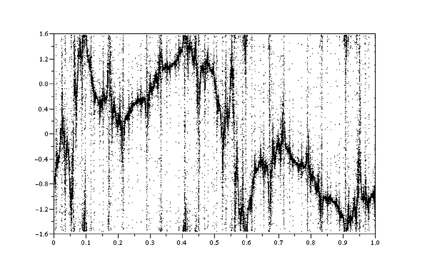
Figure 3: A trajectory of $T$

$\arctan(x)$

$\theta$

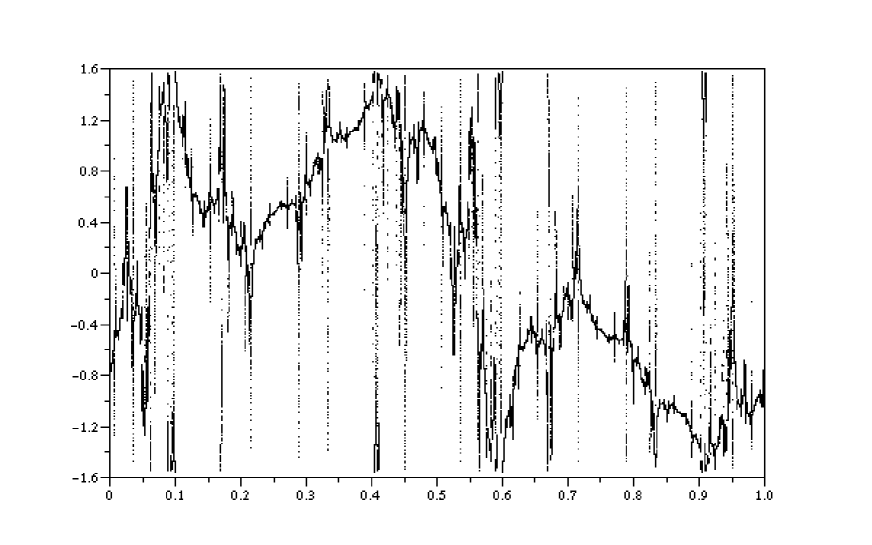
Figure 4: The invariant graph

$\arctan(x)$

$\theta$

References

• [ACO99] L. Arnold, N.D. Cong, and V.I. Oseledets. Jordan normal form for linear cocycles. Random Operators and Stochastic Equations, 7(4):303–358, 1999.
• [Arn98] L. Arnold. Random Dynamical Systems. Springer, 1998.
• [BJ02] J. Bourgain and S. Jitomimirskaya. Continuity of the Lyapunov exponent for quasiperiodic operators with analytic potential. Journal of Statistical Physics, 108(5–6):1203–1218, 2002.
• [DJKR] S. Datta, T. Jäger, G. Keller, and R. Ramaswamy. Preprint.
• [dMvS93] W. de Melo and S. van Strien. One-dimensional dynamics. Springer, 1993.
• [Fur61] H. Furstenberg. Strict ergodicity and transformation of the torus. American Journal of Mathematics, 83:573–601, 1961.
• [Her83] Michael R. Herman. Une méthode pour minorer les exposants de Lyapunov et quelques exemples montrant le caractère local d’un théorème d’Arnold et de Moser sur le tore de dimension 2. Commentarii Mathematici Helvetici, 58:453–502, 1983.
• [Jit99] S. Y. Jitomirskaya. Metal-insulator transition for the almost Mathieu operator. Annals of Mathematics (2), 150(3):1159–1175, 1999.
• [Kel96] Gerhard Keller. A note on strange nonchaotic attractors. Fundamenta Mathematicae, 151(2):139–148, 1996.
• [KH97] A. Katok and B. Hasselblatt. Introduction to the Modern Theory of Dynamical Systems. Cambridge University Press, 1997.
• [KS97] Jukka A. Ketoja and Indubala I. Satija. Harper equation, the dissipative standard map and strange nonchaotic attractors: Relationship between an eigenvalue problem and iterated maps. Physica D, 109:70–80, 1997.
• [PRSS99] Awadhesh Prasad, Ramakrishna Ramaswamy, Indubala I. Satija, and Nausheen Shah. Collision and symmetrie breaking in the transition to strange nonchaotic attractors. Physical Review Letters, 83(22):4530–4533, 1999.
• [SFGP02] J. Stark, U. Feudel, P. Glendinning, and A. Pikovsky. Rotation numbers for quasi-periodically forced monotone circle maps. Dynamical System, 17:1–28, 2002.
• [Sta03] J. Stark. Transitive sets for quasiperiodically forced monotone maps. Preprint, 2003.
• [Thi97] Ph. Thieullen. Ergodic reduction of random products of two-by-two matrices. Journal d’Analyse Mathématique, 73:19–64, 1997.