A discontinuous Galerkin formulation for a strain gradient-dependent damage model

Abstract

Keywords
Discontinuous Galerkin methods, gradient-dependent continua, damage.

1 Introduction

Strain gradient dependent continuum models have been developed for a wide range of problems. Strain gradient effects are included in continuum models to reproduce experimentally observed phenomena which cannot be captured with classical models [1, 2, 3, 5, 4, 6, 7]. The range of application is broad, from large geological problems to polycrystals. Typical phenomena which can be captured with strain gradient models include strain localisation in the presence of softening and size effects.

The development of strain gradient models has been hindered by the lack of a suitable numerical framework for their robust solution on arbitrary domains. The introduction of strain gradients into continuum models poses significant challenges in solving the ensuing equations. The finite element method, the dominant numerical method in solid mechanics, is ideally suited to the solution of second-order partial differential equations, such as classical elasticity. The solution of gradient-dependent continuum problems usually demands at least $C^{1}$ continuous basis functions, which are difficult to construct in spatial dimensions higher than one. Previous attempts to solve such problems with $C^{1}$ shape functions or ad-hoc measures have proven difficult [2, 8, 9]. More seriously, in numerous publications, basic continuity requirements are completely ignored. To avoid these difficulties, Askes et al. [10] applied the element-free Galerkin method, which can provide a high degree of continuity, for the solution of strain gradient dependent damage models. However, the element-free Galerkin method entails other difficulties, lacks the penetration in the solid mechanics community of the finite element method, and is generally less efficient. As a result of these difficulties, strain gradient dependent models are not widely applied, and many formulations are largely untested. The difficulties presented by continuity requirements has even lead to reformulations of strain gradient models that are driven by algorithmic convenience [5, 11].

In this work, a fresh perspective is taken on the solution of strain gradient dependent continuum problems in light of recent developments in discontinuous and continuous/discontinuous Galerkin methods for elliptic problems [12, 13, 14]. A summary of recent developments can be found in Arnold et al. [13]. In the derivation of the Galerkin problem, potential discontinuities in the basis functions across internal surfaces are taken into account, resulting in a generalisation of the conventional Galerkin method.

To begin, a strain gradient-dependent damage model, which is used as a prototype example, is introduced. It is cast as a continuous Galerkin problem in a finite element framework and the difficulties with the conventional finite element method are highlighted. The Galerkin problem is then generalised to allow for discontinuities in the appropriate fields. The formulation is tested for the simplest possible finite element in one dimension. A series of test cases are computed and the results are compared to a benchmark solution.

2 Gradient-enhanced damage model: Preliminaries

Consider a body $\Omega$ in $\mathbb{R}^{n}$, with boundary $\Gamma=\partial\Omega$. The strong form of the equilibrium equation for the body $\Omega$, in the absence of body forces, and associated standard boundary conditions, is:

$${\nabla}\cdot\bm{\sigma} =\bm{0} {\rm in}\ \Omega$$ (1)

$$\bm{\sigma}\cdot\bm{n} =\bm{h} {\rm on}\ \Gamma_{h}$$ (2)

$$\bm{u} =\bm{g} {\rm on}\ \Gamma_{g}$$ (3)

where ${\nabla}$ is the gradient operator, $\bm{\sigma}$ is the stress tensor, $\bm{h}$ is the prescribed traction on $\Gamma_{h}$ and $\bm{g}$ is the prescribed displacement on the boundary $\Gamma_{g}$ ($\Gamma_{g}\cup\Gamma_{h}=\Gamma$, $\Gamma_{g}\cap\Gamma_{h}=\emptyset$). The outward normal to $\Gamma$ is denoted $\bm{n}$.

For an isotropic elasticity-based damage model, the stress at a material point is given by:

$$\bm{\sigma}=\left({1-\omega}\right)\mathcal{C}\mathbf{:}{\nabla}^{\rm s}\bm{u}$$ (4)

where $\mathcal{C}$ is the usual linear-elastic constitutive tensor and the damage variable ($0\leq\omega\leq 1$) is a function of a scalar history parameter $\kappa$,

$$\omega=\omega\left({\kappa}\right).$$ (5)

The history parameter $\kappa$ is related to a gradient-dependent ‘equivalent strain’, $\overline{\epsilon}$. A common choice for $\overline{\epsilon}$ is:

$$\overline{\epsilon}=\epsilon_{\rm eq}+c^{2}\Delta\epsilon_{\rm eq}$$ (6)

where $\epsilon_{\rm eq}$ is an invariant of the local strain tensor $\bm{\epsilon}={\nabla}^{\rm s}\bm{u}$, $c$ is a length scale which reflects the strength of strain gradient effects and $\Delta$ is the Laplacian operator. This formulation is often named ‘explicit gradient damage’ [5]. The chosen invariant for the local equivalent strain reflects the processes that drive damage growth in a given material. In one dimension, the obvious choice is that the equivalent strain is equal to the strain.

The history parameter $\kappa$ is equal to the largest positive value of $\overline{\epsilon}$ reached at a material point. Defining a loading function $f$,

$$f=\overline{\epsilon}-\kappa$$ (7)

the evolution of $\kappa$ obeys the Kuhn-Tucker conditions,

$$\dot{\kappa}\geq 0, f\leq 0, \dot{\kappa}f=0.$$ (8)

A commonly adopted dependency is:

$$\omega=\begin{cases}0&{\rm if}\ \ \kappa\leq\kappa_{0}\\ 1-\dfrac{\kappa_{0}\left({\kappa_{c}-\kappa}\right)}{\kappa\left({\kappa_{c}-\kappa_{0}}\right)}&{\rm if}\ \ \kappa_{0}<\kappa<\kappa_{c}\\ 1&{\rm if}\ \ \kappa\geq\kappa_{c}\end{cases}$$ (9)

where $\kappa_{0}$ is the value of the history parameter at which damage begins to develop and $\kappa_{c}$ is the value at which $\omega=1$. The evolution of $\omega$ in equation (9) yields a linear softening response for a uniaxial test in the absence of strain gradient effects. To make the dependency of $\omega$ on $\overline{\epsilon}$ clear, the expressions $\omega\left({\kappa}\right)$ and $\omega\left({\overline{\epsilon}}\right)$ will be used interchangeably.

Insertion of the constitutive model (see equations (4), (5) and (6)) into the equilibrium equation (1) leads to a non-linear fourth-order partial differential equation. This requires the prescription of boundary conditions on gradients of the displacement field higher than one. The physical implications of these boundary conditions are unclear and are the subject of debate. At this stage, the boundary condition

$$c^{2}{\nabla}\epsilon_{\rm eq}\cdot\bm{n}=\epsilon_{\rm bc} {\rm on}\ \Gamma$$ (10)

is considered. A common choice is $\epsilon_{\rm bc}=0$, which is adopted for all examples in Section 4.

This elasticity-based damage model is convenient for preliminary developments as $\epsilon_{\rm eq}$ is calculated explicitly from the gradient of the displacement field, which is in contrast to the equivalent plastic strain in an elastoplastic model. However, equation (6) is identical in form to the equation for the gradient-dependent equivalent plastic strain that is adopted in many strain gradient dependent plasticity models [1, 3, 7]. This model therefore provides a canonical formulation which can be extended to a broader class of models.

3 Galerkin formulation

In developing a weak formulation for eventual finite element solution, the equilibrium equation (1) and the equation for $\overline{\epsilon}$ (6) are considered separately. The non-linear fourth-order equation resulting from insertion of the constitutive equations into the equilibrium equation could potentially be cast in a weak from. The formulation would inevitably be specific to the chosen dependency of damage on $\overline{\epsilon}$, a dependency which is potentially highly complex. Hence, for simplicity and generality, it is convenient to treat the two equations separately.

The body $\Omega$ is partitioned into $n_{el}$ non-overlapping elements $\Omega_{e}$ such that

$$\overline{\Omega}=\bigcup_{e=1}^{n_{el}}\overline{\Omega}_{e}.$$ (11)

where $\overline{\Omega}_{e}$ is a closed set (i.e., it includes the boundary of the element). The elements $\Omega_{e}$ (which are open sets) satisfy the standard requirements for a finite element partition. A domain $\widetilde{\Omega}$ is also defined

$$\widetilde{\Omega}=\bigcup_{e=1}^{n_{el}}\Omega_{e}$$ (12)

where $\widetilde{\Omega}$ does not include element boundaries. It is also useful to define the ‘interior’ boundary $\widetilde{\Gamma}$,

$$\widetilde{\Gamma}=\bigcup_{i=1}^{n_{b}}\Gamma_{i}$$ (13)

where $\Gamma_{i}$ is the $i$th interior element boundary and $n_{b}$ is the number of internal inter-element boundaries.

Consider now the function spaces $\mathcal{S}^{h}$, $\mathcal{V}^{h}$ and $\mathcal{W}^{h}$,

$$\mathcal{S}^{h} =\left\{{u^{h}_{i}\in H_{0}^{1}\left({\Omega}\right)\ \left|\ u_{i}^{h}|_{\Omega_{e}}\in P_{k_{1}}\left({\Omega_{e}}\right)\forall e,\ u_{i}=g_{i}\ {\rm on}\ \Gamma_{g}\right.}\right\}$$ (14)

$$\mathcal{V}^{h} =\left\{{w^{h}_{i}\in H_{0}^{1}\left({\Omega}\right)\ \left|\ w_{i}^{h}|_{\Omega_{e}}\in P_{k_{1}}\left({\Omega_{e}}\right)\forall e,\ w_{i}=0\ {\rm on}\ \Gamma_{g}\right.}\right\}$$ (15)

$$\mathcal{W}^{h} =\left\{{q^{h}\in L_{2}\left({\Omega}\right)\ \left|\ q^{h}|_{\Omega_{e}}\in P_{k_{2}}\left({\Omega_{e}}\right)\forall e\right.}\right\}$$ (16)

where $P_{k}$ represents the space of polynomial finite element shape functions (of polynomial order $k$). The spaces $\mathcal{S}^{h}$ and $\mathcal{V}^{h}$ represent usual $C^{0}$ continuous finite element shape functions. The space $\mathcal{W}^{h}$ can contain discontinuous functions.

3.1 Standard Galerkin weak form

The standard, continuous Galerkin problem for the equilibrium equation (1) is of the form: Find $\bm{u}^{h}\in\mathcal{S}^{h}$ such that

$$\int_{\Omega}{\nabla}\bm{w}^{h}\mathbf{:}\left({1-\omega\left({\overline{\epsilon}^{h}}\right)}\right)\mathcal{C}\mathbf{:}{\nabla}^{\rm s}\bm{u}^{h}\ d\Omega-\int_{\Gamma_{h}}\bm{w}^{h}\cdot\bm{h}\ d\Gamma=0 \forall\bm{w}^{h}\in\mathcal{V}^{h}$$ (17)

where it was already assumed that $\bm{u}^{h}$ is $C^{0}$ continuous (see equation (14)). Note that the damage is a function of $\overline{\epsilon}$, which is in turn a function of displacement gradients, making the equation non-linear. It is presumed at this point that $\overline{\epsilon}^{h}$ is square-integrable over $\Omega$ ($\overline{\epsilon}^{h}\in L_{2}\left({\Omega}\right)$).

A second Galerkin problem is constructed to solve for $\overline{\epsilon}$ (equation (6)). It consists of: Find $\overline{\epsilon}\in\mathcal{W}^{h}$ such that

$$\int_{\Omega}q^{h}\overline{\epsilon}^{h}\ d\Omega-\int_{\Omega}q^{h}\epsilon_{\rm eq}^{h}\ d\Omega+\int_{\Omega}{\nabla}q^{h}\cdot c^{2}{\nabla}\epsilon_{\rm eq}^{h}\ d\Omega-\int_{\Gamma}q^{h}\epsilon_{\rm bc}\ d\Gamma=0\ \ \ \ \forall q^{h}\in\mathcal{W}^{h}$$ (18)

where it is assumed that $\epsilon_{\rm eq}^{h}$ is known. Recall that discontinuities in $q^{h}$ and $\overline{\epsilon}^{h}$ are permitted.

Two difficulties exist in the preceding Galerkin formulation. The first is that the weight function $q^{h}$ can be discontinuous (cf. equation (16)), meaning that ${\nabla}q^{h}$ is not necessarily square-integrable on $\Omega$. This problem can be circumvented easily by requiring $C^{0}$ continuity of the functions in $\mathcal{W}^{h}$. The second problem, which is less easily solved, is that $\epsilon_{\rm eq}^{h}$ is computed from ${\nabla}^{\rm s}\bm{u}^{h}$. Therefore, calculating ${\nabla}\epsilon_{\rm eq}^{h}$ everywhere in $\Omega$ requires that the displacement field $\bm{u}^{h}$ be $C^{1}$ continuous if singularities are to be avoided. However, since $\bm{u}^{h}\in H^{1}_{0}\left({\Omega}\right)$ (see equation (14)), it is not necessarily $C^{1}$ continuous.

To proceed with this formulation in a conventional manner, two possibilities present themselves. The first is to solve equations (17) and (18) using $C^{0}$ finite element shape functions to interpolate $\overline{\epsilon}^{h}$ and $q^{h}$, which is straightforward, and using $C^{1}$ shape functions for $\bm{w}^{h}$ and $\bm{u}^{h}$. The second approach is to interpolate $\epsilon_{\rm eq}$ using $C^{1}$ shape functions, from which the term $\Delta\epsilon_{\rm eq}$ can be evaluated everywhere in $\Omega$. The second approach may appear more attractive than the first as it requires a $C^{1}$ interpolation of a scalar field rather than a vector field. Both approaches pose significant difficulties as $C^{1}$ shape functions are difficult to construct, lack generality and lead to extremely complex element formulations. $C^{1}$ functions are difficult to construct in two dimensions, and to the authors’ knowledge, untried in three dimensions.

3.2 Discontinuous Galerkin form

The approach advocated here avoids the need for $C^{1}$ continuity of the displacement field by imposing the required degree of continuity in a weak sense. Before proceeding with the formulation, it is necessary to define jump and an averaging operations. The jump in a field $\bm{a}$ across a surface (which is associated with a body) is given by [13]:

$$\left\llbracket{\bm{a}}\right\rrbracket=\bm{a}_{1}\cdot\bm{n}_{1}+\bm{a}_{2}\cdot\bm{n}_{2}$$ (19)

where the subscripts denote the side of the surface and $\bm{n}$ is the outward unit normal vector. This definition is convenient as it avoids introducing ‘+’ and ‘-’ sides of a surface. This is particularly so for arbitrarily-oriented surfaces in two and three dimensions. The average of a field $\bm{a}$ across a surface is given by:

$$\left<{\bm{a}}\right>=\frac{\left({\bm{a}_{1}+\bm{a}_{2}}\right)}{2}.$$ (20)

Consider now equation (6) for $\overline{\epsilon}$, which can be cast in a weak form using integration by parts and the divergence theorem on the boundary $\Gamma$ and on inter-element boundaries, $\widetilde{\Gamma}$. This yields:

$$\int_{\Omega}q^{h}\overline{\epsilon}^{h}\ d\Omega-\int_{\Omega}q^{h}\epsilon_{\rm eq}^{h}\ d\Omega+\int_{\widetilde{\Omega}}{\nabla}q^{h}\cdot c^{2}{\nabla}\epsilon_{\rm eq}^{h}\ d\Omega-\int_{\Gamma}q^{h}\epsilon_{\rm bc}\ d\Gamma\\ -\int_{\widetilde{\Gamma}}\left<{q^{h}}\right>\cdot c^{2}\left\llbracket{{\nabla}\epsilon_{\rm eq}^{h}}\right\rrbracket\ d\Gamma-\int_{\widetilde{\Gamma}}\left\llbracket{q^{h}}\right\rrbracket\cdot c^{2}\left<{{\nabla}\epsilon_{\rm eq}^{h}}\right>\ d\Gamma=0.$$ (21)

Note the distinction between $\Omega$ and $\widetilde{\Omega}$ for the volume integrals. It is chosen that the following weak statements of continuity should hold:

$$\int_{\widetilde{\Gamma}}\left<{q^{h}}\right>c^{2}\left\llbracket{{\nabla}\epsilon_{\rm eq}^{h}}\right\rrbracket\ d\Gamma =0 \forall q^{h}\in\mathcal{W}^{h}$$ (22)

$$-\int_{\widetilde{\Gamma}}\left<{{\nabla}q^{h}}\right>\cdot c^{2}\left\llbracket{\epsilon_{\rm eq}^{h}}\right\rrbracket\ d\Gamma =0 \forall q^{h}\in\mathcal{W}^{h}.$$ (23)

Also, a ‘penalty-like’ term is introduced:

$$\int_{\widetilde{\Gamma}}\frac{c^{2}}{h_{e}}\left\llbracket{q^{h}}\right\rrbracket\cdot{\left\llbracket{\epsilon_{\rm eq}^{h}}\right\rrbracket}\ d\Gamma=0$$ (24)

where $h_{e}$ is a length scale which is required for dimensional consistency. Adding the additional equations to equation (21) leads to the following Galerkin problem: Find $\overline{\epsilon}^{h}\in\mathcal{W}^{h}$ such that

$$\int_{\Omega}q^{h}\overline{\epsilon}^{h}\ d\Omega-\int_{\Omega}q^{h}\epsilon_{\rm eq}^{h}\ d\Omega+\int_{\widetilde{\Omega}}{\nabla}q^{h}\cdot c^{2}{\nabla}\epsilon_{\rm eq}^{h}\ d\Omega-\int_{\Gamma}q^{h}\epsilon_{\rm bc}\ d\Gamma\\ -\int_{\widetilde{\Gamma}}\left\llbracket{q^{h}}\right\rrbracket\cdot c^{2}\left<{{\nabla}\epsilon_{\rm eq}^{h}}\right>\ d\Gamma-\int_{\widetilde{\Gamma}}\left<{{\nabla}q^{h}}\right>\cdot c^{2}\left\llbracket{\epsilon_{\rm eq}^{h}}\right\rrbracket\ d\Gamma\\ +\int_{\widetilde{\Gamma}}\frac{c^{2}}{h_{e}}\left\llbracket{q^{h}}\right\rrbracket\cdot{\left\llbracket{\epsilon_{\rm eq}^{h}}\right\rrbracket}\ d\Gamma=0\ \ \ \ \forall q^{h}\in\mathcal{W}^{h}.$$ (25)

Adding the term in equation (23) to the problem provides a degree of ‘symmetry’ with the term $\int_{\widetilde{\Gamma}}\left\llbracket{q^{h}}\right\rrbracket\cdot c^{2}\left<{{\nabla}\epsilon_{\rm eq}^{h}}\right>\ d\Gamma$. The choice of $c^{2}/h_{e}$ may seem somewhat arbitrary considering that it appears as a penalty-like parameter. This choice will be justified later through an analogy between the proposed method and a finite difference scheme. No gradients of $\epsilon_{\rm eq}^{h}$ or $q^{h}$ appear in terms integrated over $\Omega$ (which includes interior boundaries) in equation (25), hence the continuity requirements on the spaces $\mathcal{S}^{h}$ and $\mathcal{W}^{h}$ are sufficient.

Equation (25) reassembles the ‘interior penalty’ method for classical elasticity, which belongs to the discontinuous Galerkin family of methods [13]. Terms have been added to the weak form that for a conventional elasticity problem would lead to a symmetric formulation. Symmetry is however not of relevance here as the functions $q^{h}$ and $\epsilon_{\rm eq}^{h}$ will generally come from different function spaces. This formulation is general for the case in which the space $\mathcal{W}^{h}$ contains discontinuous functions. However, note if all functions in the space $\mathcal{W}^{h}$ are $C^{0}$ continuous, the formulation is still valid, with terms relating to the jump in $\epsilon^{h}$ remaining. The formulation would then resemble a continuous/discontinuous Galerkin method [14].

The solution of the gradient enhanced damage problem requires the simultaneous solution of equations (17) and (25), which are coupled. In summary, the problem is: Find $\bm{u}^{h}\in\mathcal{S}^{h}$ and $\overline{\epsilon}^{h}\in\mathcal{W}^{h}$ such that

$$\int_{\Omega}{\nabla}\bm{w}^{h}\mathbf{:}\left({1-\omega\left({\overline{\epsilon}^{h}}\right)}\right)\mathcal{C}\mathbf{:}{\nabla}^{\rm s}\bm{u}^{h}\ d\Omega-\int_{\Gamma_{h}}\bm{w}^{h}\cdot\bm{h}\ d\Gamma=0 \forall\bm{w}^{h}\in\mathcal{V}^{h}$$ (26)

$$\int_{\Omega}q^{h}\overline{\epsilon}^{h}\ d\Omega-\int_{\Omega}q^{h}\epsilon_{\rm eq}^{h}\ d\Omega+\int_{\widetilde{\Omega}}{\nabla}q^{h}\cdot c^{2}{\nabla}\epsilon_{\rm eq}^{h}\ d\Omega-\int_{\Gamma}q^{h}\epsilon_{\rm bc}\ d\Gamma\\ -\int_{\widetilde{\Gamma}}\left\llbracket{q^{h}}\right\rrbracket\cdot c^{2}\left<{{\nabla}\epsilon_{\rm eq}^{h}}\right>\ d\Gamma-\int_{\widetilde{\Gamma}}\left<{{\nabla}q^{h}}\right>\cdot c^{2}\left\llbracket{\epsilon_{\rm eq}^{h}}\right\rrbracket\ d\Gamma\\ +\int_{\widetilde{\Gamma}}\frac{c^{2}}{h_{e}}\left\llbracket{q^{h}}\right\rrbracket\cdot{\left\llbracket{\epsilon_{\rm eq}^{h}}\right\rrbracket}\ d\Gamma=0\ \ \ \ \forall q^{h}\in\mathcal{W}^{h}$$ (27)

where the nonlinear equations are coupled through the dependency of $\omega$ on $\overline{\epsilon}^{h}$ and the dependency of $\overline{\epsilon}^{h}$ on $\bm{u}^{h}$. Linearisation of these equations is straightforward, and is included in Appendix A.

In this work, the simplest possible finite element formulation is considered. It is chosen to interpolate the displacement field with linear piecewise continuous ($C^{0}$) functions and to use constant functions on elements for $\overline{\epsilon}$ ($k_{2}=0$ in equation (16)). Also, the boundary condition ${\nabla}\epsilon_{\rm eq}\cdot\bm{n}=0$ on $\Gamma$ is applied. As a consequence, several terms disappear from equation (27), leading to the problem: Find $\overline{\epsilon}^{h}\in\mathcal{W}^{h}$ such that

$$\int_{\Omega}q^{h}\overline{\epsilon}^{h}\ d\Omega-\int_{\Omega}q^{h}\epsilon_{\rm eq}^{h}\ d\Omega+\int_{\widetilde{\Gamma}}\frac{c^{2}}{h_{e}}\left\llbracket{q^{h}}\right\rrbracket\cdot{\left\llbracket{\epsilon_{\rm eq}^{h}}\right\rrbracket}\ d\Gamma=0 \forall q^{h}\in\mathcal{W}^{h}.$$ (28)

If $c=0$, $\overline{\epsilon}=\epsilon_{\rm eq}$ at all points in $\Omega$, and the model reduces to a local damage formulation (no gradient effects). In one dimension, $h_{e}$ is taken as $\left<{h_{e}}\right>$. A higher-dimension generalisation would be the distance between the centroid of the neighbouring elements.

A physical interpretation of equation (28) is simple. The stronger the spatial variation in the strain field , the larger the jumps in the strain across element boundaries. Equation (28) sets $\overline{\epsilon}$ equal to the local equivalent strain, and subtracts a component which is proportional to the equivalent strain jump and the material parameter $c^{2}$, effectively decreasing $\overline{\epsilon}$ (relative the $\epsilon_{\rm eq}$) in the presence of rapid spatial variation in the strain field, which is manifest in the form of jumps in the strain across element boundaries.

In practice, this finite element formulation is very simple. An element has three nodes. Displacement degrees of freedom are located at the two end-nodes, and a degree of freedom for $\overline{\epsilon}$ is located at the centre node of each element. The standard loop over all elements in a mesh is performed, and in addition all interior interfaces are looped over. Despite the node corresponding to $\overline{\epsilon}^{h}$ being internal to an element, it cannot be eliminated at the element level. The element stiffness matrices for this formulation are elaborated in Appendix B.

3.3 Consistency of the discontinuous formulation

Having added non-standard terms to the weak form, it is important to prove consistency of the method. Applying integration by parts to the integral over $\widetilde{\Omega}$ in equation (25),

$$\int_{\widetilde{\Omega}}{\nabla}q^{h}\cdot c^{2}{\nabla}\epsilon_{\rm ep}^{h}\ d\Omega=-\int_{\widetilde{\Omega}}q^{h}c^{2}\Delta\epsilon_{\rm eq}^{h}\ d\Omega+\int_{\Gamma}q^{h}c^{2}{\nabla}\epsilon_{\rm eq}\cdot\bm{n}\ d\Gamma\\ +\int_{\widetilde{\Gamma}}\left<{q^{h}}\right>c^{2}\left\llbracket{{\nabla}\epsilon_{\rm eq}}\right\rrbracket\ d\Gamma+\int_{\widetilde{\Gamma}}\left\llbracket{q^{h}}\right\rrbracket\cdot c^{2}\left<{{\nabla}\epsilon_{\rm eq}}\right>\ d\Gamma.$$ (29)

Inserting this expression into the infinite-dimensional version of equation (25), and employing standard variational arguments, the following Euler-Lagrange equations can be identified:

$$\overline{\epsilon}-\epsilon_{\rm eq}-c^{2}\Delta\epsilon_{\rm eq} =0 {\rm in}\ \ \widetilde{\Omega}$$ (30)

$$c^{2}\left\llbracket{\epsilon_{\rm eq}}\right\rrbracket =0 {\rm on}\ \ \widetilde{\Gamma}$$ (31)

$$c^{2}\left\llbracket{{\nabla}\epsilon_{\rm eq}}\right\rrbracket =0 {\rm on}\ \ \widetilde{\Gamma}$$ (32)

$$c^{2}{\nabla}\epsilon_{\rm eq}\cdot\bm{n} =\epsilon_{\rm bc} {\rm on}\ \ \Gamma$$ (33)

Equation (30) is the original problem over element interiors (see equation (1)). Equations (31) and (32) impose continuity of the corresponding fields across element boundaries and equation (33) imposes the natural boundary condition on ${\nabla}\epsilon_{\rm eq}\cdot\bm{n}$. The Galerkin form (equation (25)) can therefore be seen as the weak imposition of these Euler-Lagrange equations.

3.4 Finite difference analogy

In one-dimension for equally spaced nodal points, it can be shown that the proposed formulation ($C^{0}$ linear $u^{h}$ and piecewise constant $\overline{\epsilon}^{h}$) is equivalent to a finite difference scheme for calculating $\epsilon_{{\rm eq},xx}$ (which is equal to $u_{,xxx}$ for $\epsilon_{\rm eq}=u_{,x}$) at the centre of each element.

Consider the two element configuration in figure 1.

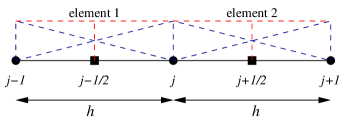
Figure 1: Two element configuration. Displacement degrees of freedom are located at the circular nodes, and $\overline{\epsilon}$ degrees of freedom are located at the squares.

The displacement degrees of freedom are stored at the circular nodes and are denoted $a_{j}$. From the form of the finite element shape functions, the jump in the equivalent strain at element boundary $j$ is given by:

$$\left.\frac{1}{h}\left\llbracket{\epsilon^{h}_{\rm eq}}\right\rrbracket\right|_{j}=-\frac{a_{j-1}-2a_{j}+a_{j+1}}{h^{2}}=-u^{\prime\prime}|_{j}$$ (34)

which is equivalent to the second-order finite difference expression for the second derivative of the displacement field $j$. From equation (28), if the displacement field is known, $\overline{\epsilon}^{h}$ for an element is equal to:

$$\begin{split}q^{h}\overline{\epsilon}^{h}&=q^{h}\epsilon^{h}_{\rm eq}-\left.\frac{c^{2}}{h^{2}}\left\llbracket{q^{h}}\right\rrbracket\left\llbracket{\epsilon^{h}_{\rm eq}}\right\rrbracket\right|_{j-1}-\left.\frac{c^{2}}{h^{2}}\left\llbracket{q^{h}}\right\rrbracket\left\llbracket{\epsilon^{h}_{\rm eq}}\right\rrbracket\right|_{j}\\[4.30554pt] &=q^{h}\left({\epsilon^{h}_{\rm eq}+\left.\frac{c^{2}}{h^{2}}\left\llbracket{\epsilon^{h}_{\rm eq}}\right\rrbracket\right|_{j-1}-\left.\frac{c^{2}}{h^{2}}\left\llbracket{\epsilon^{h}_{\rm eq}}\right\rrbracket\right|_{j}}\right)\end{split}$$ (35)

This is equivalent to:

$$\overline{\epsilon}^{h}=\epsilon^{h}_{\rm eq}+\frac{c^{2}}{h}\left({\left.u^{\prime\prime}\right|_{j}-\left.u^{\prime\prime}\right|_{j-1}}\right)$$ (36)

which is a finite difference approximation of equation (6), showing that the proposed variational formulation is identical to a finite-difference procedure in one-dimension for the case of equally spaced nodal points.

4 Numerical examples

Numerical examples is this section are intended to demonstrate the objectivity of the formulation with respect to mesh refinement for strain softening problems, and to compare the computed results against a known benchmark. It is well-known that classical, rate-independent continuum models are ill-posed when strain softening is introduced, which becomes evident in a severe sensitivity of the computed result to the spatial discretisation. One motivation for strain gradient dependent model is to provide regularisation in the presence of strain softening in order to avoid pathological mesh dependency.

For all examples, the evolution of damage is given by equation (9). The materials parameters are taken as: Young’s modulus $E=20\times 10^{3}$ MPa, $\kappa_{0}=0.0001$, $\kappa_{c}=0.0125$ and $c=1$ mm. A Newton-Raphson procedure under displacement control is used to solve the problem and the governing equations have been linearised consistently.

4.1 Objectivity with respect to spatial discretisation

The first test is for objectivity of the load–displacement response with respect to mesh refinement. A tapered bar (figure 2) is tested in tension. The bar has a cross-sectional area of one square unit at each end, and tapers linearly towards the centre where the area is 0.8 square units. A displacement is applied incrementally at the right-hand end.

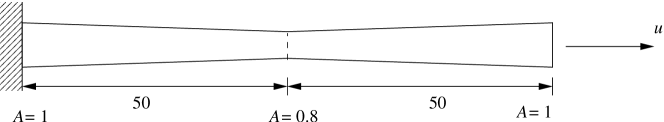
Figure 2: Linearly tapering bar.

The response is examined for meshes with 100, 200 and 400 elements. For each mesh, all elements are of equal size.

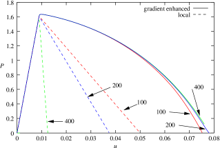
Figure 3: Load-displacement response for the tapered bar.

Responses for the three meshes are shown in figure 3 for both $c=1$ and $c=0$. Clearly, the introduction of strain gradient effects has regularised the problem, with the response for the three cases with $c=1$ being near identical. The response is further examined by comparing the damage profiles along the bar for the three regularised cases. The damage profiles, shown in figure 4, are indistinguishable for the three meshes.

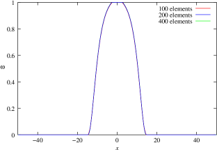
Figure 4: Damage profiles for the tapered bar.

4.2 Comparison with a high-order of continuity numerical method

The second test involves a bar with a narrow section at the centre, as shown in figure 5. This problem was previously computed for the same strain gradient dependent damage model using an element-free Galerkin method, which provides a high degree of continuity [10].

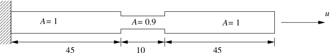
Figure 5: Bar with narrow central section.

This problem is computed using meshes with the same number of elements as the previous example. For comparison, the computed load-displacement response from an element-free Galerkin method is also included [10] for this problem. It is clear from figure 6 that the three meshes yield near-identical results and match the element-free Galerkin solution well.

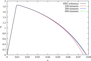
Figure 6: Load-displacement response.

The damage profiles along the bar are shown in figure 7. The damage profile from Askes et al. [10] is included as a reference.

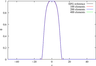
Figure 7: Damage profiles along the bar.

The computed results for all meshes are in excellent agreement with the benchmark.

5 Conclusions

A discontinuous Galerkin formulation has been developed for a strain gradient-dependent continuum model. The problem is split into two fields – the displacement and a deformation measure – for generality. The scalar field, which is a measure of the deformation, is dependent on gradients of the strain field. Conventionally, this would require a $C^{1}$ finite element interpolation of the displacement field. By including element interface terms in the Galerkin formulation, the need for high-order continuity is circumvented.

The proposed formulation was tested for the simplest element configuration in one dimension – piecewise continuous linear displacement and discontinuous piecewise constant for the extra scalar field. For simple tests, the regularising properties of the strain gradient dependent model were demonstrated and the results compared excellently with a benchmark result computed using a numerical method with a high degree of continuity. These preliminary results are promising and should be extended for higher-oder elements and to multiple spatial dimensions. For the simple formulation adopted here, several terms in the weak from could be discarded. The importance of these terms must be assessed for higher-order interpolations. This work provides a first step towards a simple and well-founded finite element framework for modern strain gradient continuum models.

Appendix A Linearisation

Effective solution of problems requires the consistent linearisation of the Galerkin problem. For the formulation, the fundamental unknowns are the displacement $\bm{u}^{h}$ and $\overline{\epsilon}^{h}$. Linearisation requires expressing the problem in terms of increments of the two unknowns. Taking the directional derivative of equation (26),

$$\int_{\Omega}{\nabla}\bm{w}^{h}\mathbf{:}\left({1-\omega}\right)\mathcal{C}\mathbf{:}\Delta\bm{\epsilon}\ d\Omega-\int_{\Omega}{\nabla}\bm{w}^{h}\mathbf{:}\frac{\partial\omega}{\partial\overline{\epsilon}}\mathcal{C}\mathbf{:}\bm{\epsilon}\Delta\overline{\epsilon}^{h}\ d\Omega=\int_{\Gamma_{h}}\bm{w}^{h}\cdot\Delta\bm{h}\ d\Gamma$$ (37)

where $\Delta\left({\cdot}\right)$ indicates a change in $\left({\cdot}\right)$. For brevity $\Delta\left({{\nabla}^{\rm s}\bm{u}^{h}}\right)$ is expressed as $\Delta\bm{\epsilon}^{h}$. Since the gradient is a linear operator, $\Delta\left({{\nabla}^{\rm s}\bm{u}}\right)={\nabla}^{\rm s}\left({\Delta\bm{u}}\right)$. Similarly, equation (27) is linearised by taking the directional derivative,

$$\int_{\Omega}q^{h}\Delta\overline{\epsilon}^{h}\ d\Omega-\int_{\Omega}q^{h}\frac{\partial\epsilon_{\rm eq}}{\partial\bm{\epsilon}}\mathbf{:}\Delta\bm{\epsilon}^{h}\ d\Omega+\int_{\widetilde{\Omega}}{\nabla}q^{h}\cdot c^{2}{\nabla}\left({\frac{\partial\epsilon_{\rm eq}}{\partial\bm{\epsilon}}\mathbf{:}\Delta\bm{\epsilon}^{h}}\right)\ d\Omega\\ -\int_{\widetilde{\Gamma}}\left\llbracket{q^{h}}\right\rrbracket\cdot c^{2}\left<{{\nabla}\left({\frac{\partial\epsilon_{\rm eq}}{\partial\bm{\epsilon}}\mathbf{:}\Delta\bm{\epsilon}^{h}}\right)}\right>\ d\Gamma-\int_{\widetilde{\Gamma}}\left<{{\nabla}q^{h}}\right>\cdot c^{2}\left\llbracket{\frac{\partial\epsilon_{\rm eq}}{\partial\bm{\epsilon}}\mathbf{:}\Delta\bm{\epsilon}^{h}}\right\rrbracket\ d\Gamma\\ +\int_{\widetilde{\Gamma}}\frac{c^{2}}{h_{e}}\left\llbracket{q^{h}}\right\rrbracket\cdot\left\llbracket{\frac{\partial\epsilon_{\rm eq}}{\partial\bm{\epsilon}}\mathbf{:}\Delta\bm{\epsilon}^{h}}\right\rrbracket\ d\Gamma=\int_{\Gamma}q^{h}\Delta\epsilon_{\rm bc}\ d\Gamma.$$ (38)

Appendix B Finite element formulation

The finite element formulation is elaborated here for the case of piecewise continuous linear $\bm{u}^{h}$ and piecewise constant $\overline{\epsilon}^{h}$. It can be extended to the more general case of arbitrary interpolation orders.

Formulation of the stiffness matrix consists of two keys steps. The first is the usual loop over all elements. This yields a stiffness matrix for each element $\bm{k}_{e}$ of the form

$$\bm{k}_{e}=\begin{bmatrix}\bm{k}_{uu}&\bm{k}_{u\overline{\epsilon}}\\ \bm{k}_{\overline{\epsilon}u}&\bm{k}_{\overline{\epsilon}\overline{\epsilon}}\end{bmatrix}$$ (39)

where the components of the matrix $\bm{k}_{e}$ are

$$\bm{k}_{uu} =\int_{\Omega_{e}}\left({1-\omega}\right){\bm{B}}^{\text{T}}\bm{D}\bm{B}\ d\Omega$$ (40)

$$\bm{k}_{u\overline{\epsilon}} =-\int_{\Omega_{e}}{\bm{B}}^{\text{T}}\frac{\partial\omega}{\partial\overline{\epsilon}}\bm{D}\bm{\epsilon}\bm{N}_{\overline{\epsilon}}\ d\Omega$$ (41)

$$\bm{k}_{\overline{\epsilon}u} =-\int_{\Omega_{e}}{\bm{N}}^{\text{T}}_{\overline{\epsilon}}{\left({\frac{\partial\epsilon_{\rm eq}}{\partial\bm{\epsilon}}}\right)}^{\text{T}}\bm{B}\ d\Omega$$ (42)

$$\bm{k}_{\overline{\epsilon}\overline{\epsilon}} =\int_{\Omega_{e}}{\bm{N}}^{\text{T}}_{\overline{\epsilon}}\bm{N}_{\overline{\epsilon}}\ d\Omega$$ (43)

where $\bm{B}$ is the usual finite element matrix containing spatial derivatives of the shape functions related to the displacement field, $\bm{D}$ is the elastic constitutive tensor in matrix form and $\bm{N}_{\overline{\epsilon}}$ contains the shape functions relating the $\overline{\epsilon}$. The strain is expressed in engineering column vector format. Once formed, an element element stiffness matrix is assembled into the global system of equations as usual.

The next, non-standard, step is a loop over all element interfaces. For this, ‘information’ is required for both the elements that are connect to the interface. The stiffness matrix at the interface two equal-order elements is twice the size of the stiffness matrix of a single element. It can be expressed as:

$$\bm{k}_{i}=\begin{bmatrix}\bm{k}_{u_{1}u_{1}}&\bm{k}_{u_{1}\overline{\epsilon}_{1}}&\bm{k}_{u_{1}u_{2}}&\bm{k}_{u_{1}\overline{\epsilon}_{2}}\\ \bm{k}_{\overline{\epsilon}_{1}u_{1}}&\bm{k}_{\overline{\epsilon}_{1}\overline{\epsilon}_{1}}&\bm{k}_{\overline{\epsilon}_{1}u_{2}}&\bm{k}_{\overline{\epsilon}_{1}\overline{\epsilon}_{2}}\\ \bm{k}_{u_{2}u_{1}}&\bm{k}_{u_{2}\overline{\epsilon}_{1}}&\bm{k}_{u_{2}u_{2}}&\bm{k}_{u_{2}\overline{\epsilon}_{2}}\\ \bm{k}_{\overline{\epsilon}_{2}u_{1}}&\bm{k}_{\overline{\epsilon}_{2}\overline{\epsilon}_{1}}&\bm{k}_{\overline{\epsilon}_{2}u_{2}}&\bm{k}_{\overline{\epsilon}_{2}\overline{\epsilon}_{2}}\end{bmatrix}$$ (44)

where the subscripts ‘1’ and ‘2’ denote the element on either side of the surface. For the case of linear $\bm{u}^{h}$ and constant $\overline{\epsilon}$, only the terms $\bm{k}_{\overline{\epsilon}_{j}u_{k}}$ are non-zero. It is equal to:

$$\bm{k}_{\overline{\epsilon}_{j}u_{k}}=\int_{\widetilde{\Gamma}_{i}}\frac{c^{2}}{h_{e}}{\bm{N}}^{\text{T}}_{\overline{\epsilon}j}{\bm{n}}^{\text{T}}_{j}\bm{n}_{k}{\left({\frac{\partial\epsilon_{\rm eq}}{\partial\bm{\epsilon}}}\right)}^{\text{T}}\bm{B}_{k}\ d\Gamma$$ (45)

where the indices $j$ and $k$ run from one to two, corresponding to sides of the interface. Note that in the usual case of $\bm{n}_{1}=-\bm{n}_{2}$, ${\bm{n}}^{\text{T}}_{i}\bm{n}_{j}=1$ if $i=j$, and ${\bm{n}}^{\text{T}}_{i}\bm{n}_{j}=-1$ if $i\neq j$.

References

- Aifantis [1984] E. C. Aifantis, On the microstructural origin of certain inelastic models, Journal of Engineering Materials Technology 106 (1984) 326–334.
- Larsy and Belytschko [1988] D. Larsy and T. Belytschko, Localization limiters in transient problems, International Journal of Solids and Structures 24 (6) (1988) 581–597.
- Mühlhaus and Aifantis [1991] H.-B. Mühlhaus and E. C. Aifantis, A variational formulation for gradient plasticity, International Journal of Solids and Structures 28 (1991) 845–857.
- Fleck and Hutchinson [1997] N. A. Fleck and J. W. Hutchinson, Strain gradient plasticity, Advances in Applied Mechanics 33 (1997) 295–361.
- Peerlings et al. [1996] R. H. J. Peerlings, R. de Borst, W. A. M. Brekelmans and J. H. P. De Vree, Gradient enhanced damage for quasi-brittle materials, International Journal for Numerical Methods in Engineering 39 (1996) 3391–3403.
- Gao and Nix [1999] H. Gao and W. D. Nix, Mechanism-based strain gradient plasticity – I. Theory, Journal of the Mechanics and Physics of Solids 47 (1999) 1239–1263.
- Fleck and Hutchinson [2001] N. A. Fleck and J. W. Hutchinson, A reformulation of strain gradient plasticity, Journal of the Mechanics and Physics of Solids 49 (2001) 2245–2271.
- de Borst and Mühlhaus [1992] R. de Borst and H.-B. Mühlhaus, Gradient-dependent plasticity – formulation and algorithmic aspects, International Journal for Numerical Methods in Engineering 35 (3) (1992) 521–539.
- de Borst and Pamin [1996] R. de Borst and J. Pamin, Some novel developments in finite element procedures for gradient-dependent plasticity, International Journal for Numerical Methods in Engineering 39 (14) (1996) 2477–2505.
- Askes et al. [2000] H. Askes, J. Pamin and R. de Borst, Dispersion analysis and element-free Galerkin solutions of second- and fourth-order gradient-enhanced damage models, International Journal for Numerical Methods in Engineering 69 (6) (2000) 811–832.
- Engelen et al. [2003] R. A. B. Engelen, M. G. D. Geers and F. P. T. Baaijens, Nonlocal implicit gradient-enhanced elasto-plasticity for the modelling of softening behaviour, International Journal of Plasticity 19 (4) (2003) 403–433.
- Oden et al. [1998] J. T. Oden, I. Babuska and C. E. Baumann, A discontinuous hp finite element method for diffusion problems, Journal of Computational Physics 146 (2) (1998) 491–519.
- Arnold et al. [2002] D. N. Arnold, F. Brezzi, B. Cockburn and L. D. Marini, Unified analysis of discontinuous galerkin methods for elliptic problems, SIAM Journal on Numerical Analysis 39 (5) (2002) 1749–1779.
- Engel et al. [2002] G. Engel, K. Garikipati, T. J. R. Hughes, M. G. Larson and R. L. Taylor, Continuous/discontinuous finite element approximations of fourth-order elliptic problems in structural and continuum mechanics with applications to thin beams and plates, and strain gradient elasticity, Computer Methods in Applied Mechanics and Engineering 191 (34) (2002) 3669–3750.