Lagrangian Surfaces in a Fixed Homology Class:
Existence of Knotted Lagrangian Tori

Abstract. In this paper we show that there exist simply connected symplectic manifolds which contain infinitely many knotted lagrangian tori, i.e., nonisotopic lagrangian tori that are image of homotopic embeddings. Moreover, the homology class they represent can be assumed to be nontrivial and primitive. This answers a question of Eliashberg and Polterovich.

1. Introduction and statement of the results

Let $M$ be a smooth, closed $4$-manifold endowed with a symplectic form $\omega$ and let $\Sigma$ be a smooth, closed oriented surface. Consider two symplectic (resp. lagrangian) embeddings $\phi_{1}$ and $\phi_{2}$ of $\Sigma$ in $M$. Assume furthermore that the $\phi_{i}$’s are smoothly homotopic. Among these maps we can define two notions of equivalence, the second implying the first:

(E1) The $\phi_{i}$ are smoothly isotopic, i.e., there exists a smooth homotopy composed of embeddings;

(E2) The $\phi_{i}$ are symplectically isotopic, i.e., there exists a smooth isotopy composed of symplectic (resp. lagrangian) embeddings.
(In what follows, the terms homotopy and isotopy will always refer to smooth ones.)

A necessary condition for two embeddings to be equivalent under the equivalence relations above is that their images, the embedded surfaces $\Sigma_{i}:=\phi_{i}(\Sigma)$, satisfy the corresponding equivalence relation (that will be referred to with the same notation): in the case of (E1), the surfaces $\Sigma_{i}$ must be isotopic submanifolds of $M$, while in case of (E2), the surfaces $\Sigma_{i}$ must be isotopic through symplectic (resp. lagrangian) submanifolds. (Note that if the genus of $\Sigma$ is greater than $0$, these conditions could be not sufficient, as the embeddings $\phi$ and $\phi\cdot\gamma$, where $\gamma$ a selfdiffeomorphism of $\Sigma$ that is not isotopic to the identity, have the same image but could be nonisotopic.)

In what follows we will concentrate on the isotopy problem for the surfaces $\Sigma_{i}$; observe that, by a standard argument, two embeddings of a surface in a simply connected $4$-manifold $M$ are homotopic if and only if their images represent the same homology class.

A priori, the first equivalence relation belongs to differential topology, while the second one belongs to symplectic topology. However, as we assume that the embeddings are symplectic or lagrangian, in understanding (E1) we have to take into account the constraint related to the rigidity induced by this extra condition. In particular, this could prevent us from the possibility of realizing an equivalence class of embeddings with a symplectic or lagrangian representative. As we will see in the following, this rigidity can affect the existence of different classes of embeddings modulo the equivalence (E1).

The classification of embedded surfaces, modulo one of the equivalence relations above, can be defined as the symplectic (resp. lagrangian) knot problem. In particular, homologous but nonisotopic surfaces determine different knotted (in the sense of differential topology) symplectic or lagrangian surfaces, while isotopic surfaces that are not isotopic in the symplectic sense determine different symplectically knotted symplectic or lagrangian surfaces. (Note that, at least in general, there is no “unknot” i.e., a preferred representative of an homology class.)

In the recent past, a series of papers has addressed the question of determining whether two embedded symplectic surfaces representing the same homology class in a simply connected symplectic $4$-manifold $M$ must be isotopic. One motivation for the isotopy problem for symplectic manifolds comes from the analogous question for the case of complex curves on Kähler surfaces, where it is known, by classical results, that complex representatives of the same homology class are in fact isotopic. Working in this direction, Siebert and Tian have proven that a symplectic surface $\Sigma_{d}$, representing the class $d[H]$ in $H^{2}({\mathbb{P}}^{2},{\mathbb{Z}})$ (with standard notation) is symplectically isotopic to an algebraic curve of degree $d$, at least for $d\leq 17$. (Note that this result is stronger that the one holding in the Kähler case, as now we are requiring only that $\Sigma_{d}$ is symplectic.) A similar result holds for surfaces in $S^{2}\times S^{2}$. These results are presented in [Ti].

In contrast with that, Fintushel and Stern have presented a method to build nonisotopic symplectic tori representing multiples of the class of a symplectic $c$-embedded torus in a symplectic $4$-manifold (see [FS2] for precise definitions and results). Their construction, that applies to a large class of symplectic manifolds, shows in particular the existence of infinitely many nonisotopic simplectic tori representing the homology class $2m[F]$ ($m\geq 2$) for any elliptic surface $E(n)$ of fiber $F$. The latter result has been extended by the author in [V2] to cover the case of all multiples $q[F]$ (at least for $n\geq 3$); in particular, when $q=1$, we see that there exist infinitely many symplectic surfaces homologous, but nonisotopic, to a complex connected curve ($F$ itself). Etgü and Park have presented in [EtP] further constructions of nonisotopic tori (in classes with divisibility) that complement the previous ones. Examples of classes with positive self-intersection, or higher genus, are still eluding us (at least for simply connected manifolds: otherwise, see [Sm]). Some of the non-isotopy results above have been analyzed by Auroux, Donaldson and Katzarkov in [ADK], where they show that these examples (and new ones they built for the case of singular symplectic surfaces in ${\mathbb{P}}^{2}$) could be interpreted as a kind of braiding of parallel copies of a complex curve. The openness of the symplectic condition allows us to keep the submanifolds resulting from this braiding symplectic.

Considered all together, these results imply that, in suitable manifolds, infinitely many knot types can be realized by symplectic surfaces. On the other hand, the author is not aware of any example of isotopic symplectic surfaces that are symplectically knotted.

The symplectic knot problem, however, has been preceded historically by its lagrangian counterpart that, for reasons detailed below, is somewhat more subtle. This question arose, for the case of lagrangian ${\mathbb{R}}^{n}$’s in ${\mathbb{R}}^{2n}$ linear outside a ball, in the “first paper” on symplectic topology by Arnol’d (see [A]). In a more general set up, the problem has been summarized by Eliashberg and Polterovich in [ElP3].

The analogy between symplectic and lagrangian knot problems is obvious. But there are reasons that make the latter question more subtle, at least in relation to the equivalence (E1). The first (and probably less relevant) is that we can perturb the symplectic form $\omega$ on $M$ to a symplectic form $\omega_{\epsilon}$ in such a way that an essential surface $\Sigma$, lagrangian with respect to $\omega$, is symplectic with respect to $\omega_{\epsilon}$. This result, whose proof appears in Gompf ([G]), holds true also for pairs of disjoint surfaces, so that the existence of essential knotted lagrangian surfaces entails the existence of knotted symplectic surfaces. But the main reason of interest stems from the fact that the lagrangian condition is a closed one, in that respect similar to the condition of being complex. In particular the rigidity of this condition imposes constraints to the possibility of braiding copies of a lagrangian surface in the spirit of [ADK], and makes a result of existence of lagrangian knots appear more problematic.

In fact, the few results known so far point towards absence of knotted lagrangian surfaces. In [ElP1] Eliashberg and Polterovich show that when $\Sigma=S^{2}$ or $T^{2}$ a lagrangian surface in $T^{*}\Sigma$ homologous to the zero section is in fact isotopic to the zero section (this result is quite exhaustive as, by [LS], every homologically nontrivial lagrangian submanifold of $T^{*}\Sigma$ must be homologous to the zero section). With similar spirit, the authors prove that, at a local level (see [ElP2] for precise definitions and statements) lagrangian submanifolds are unknotted (in the sense of (E2)). Again, in [L] Luttinger proved that infinitely many knot types of tori in ${\mathbb{R}}^{4}$ can not be realized with lagrangian embeddings. In light of these results, Question 1.3A of [ElP2] asks whether there exist homotopic, but not symplectically isotopic, embeddings of a lagrangian surface. Clearly, examples of this kind are provided by homologous lagrangian surfaces that fail to satisfy (E1) or (E2). Seidel has answered in the positive to this question (see [Se1] and [Se2]) constructing an infinite number of lagrangian spheres, in a suitable $4$-manifold, that are isotopic but symplectically knotted, i.e., equivalent under (E1) but not under (E2).

The goal of this paper is to complete the answer to Question 1.3A of [ElP2] constructing an infinite number of knotted lagrangian tori, i.e., homologous lagrangian tori that are not equivalent under (E1). We will prove the following results:

Theorem 1.1.

Let $E(2)_{K}$ be the symplectic $4$-manifold (homotopy equivalent to $E(2)$) obtained by knot surgery on the left-handed trefoil $K$; then there exists a nontrivial primitive homology class $[R]$ such that any multiple $q[R]$, $q\geq 1$, can be represented by infinitely many mutually nonisotopic lagrangian tori.

Theorem 1.1 asserts therefore that infinitely many knot types can be realized by lagrangian embeddings.

It will be apparent from the proof that we are able in fact to prove something stronger, namely that if we denote by $R_{i}$ the lagrangian tori of Theorem 1.1, there is no diffeomorphism of pairs $(E(2)_{K},R_{i})\rightarrow(E(2)_{K},R_{j})$, even not connected to the identity, unless $i=j$.

This result can be extended without any effort to cover other classes of symplectic knot surgery manifolds, using for example the figure-eight knot, or any non-prime fibered knot containing $K$ as a summand, and many others. In fact, we expect the result to hold for all symplectic manifolds obtained by knot surgery on a fibered nontrivial knot, although the proof of this would require some modification in the proof of Theorem 1.1. We will address this problem in the future.

Using the aforementioned result of Gompf, we obtain the following Corollary:

Corollary 1.2.

The manifold $E(2)_{K}$ has a primitive homology class which can be represented by mutually nonisotopic symplectic tori.

We point out that phenomena of this kind for $E(2)_{K}$ are discussed in [FS2] and [EtP], but for homology classes with divisibility. Corollary 1.2 gives therefore the simplest (in the sense of geography) known symplectic manifold having symplectic nonisotopic tori in the same primitive homology class. Obviously, the same result obtained in Corollary 1.2 holds for all multiples of $[R]$.

We will briefly overview the ideas underlying the proof of Theorem 1.1. We will present the manifold $E(2)_{K}$ as result of link surgery over the link $L=K\cup M$ given by the knot $K$ and its meridian $M$. The link exterior $S^{3}\setminus\nu L$ fibers over $S^{1}$ with fiber $\Sigma_{L}$ given by the fiber $\Sigma_{K}$ of $K$ with a disk removed. We can obtain symplectic tori by looking at curves in $S^{3}\setminus\nu L$ transverse to $\Sigma_{L}$. This is the approach of all available constructions of symplectic knots. Here, we will proceed instead in the opposite way: Let $\gamma$ be a curve in $\Sigma_{L}$. Denote by $N_{K}$ the fibered $3$-manifold obtained by surgery on $K\cup M$ with coefficients $0$ and $\infty$ respectively. Then the torus $S^{1}\times\gamma$ is a lagrangian, framed torus in the manifold $S^{1}\times N_{K}$ (endowed of a standard symplectic structure). By symplectic fiber summing two copies of $E(1)$ to $S^{1}\times N_{K}$, this torus defines a framed lagrangian torus in $E(2)_{K}$. The problem at this point is reduced to find infinitely many curves $\gamma\in\Sigma_{L}$ homologous (but nonisotopic) in $S^{3}\setminus\nu L$, and then try to distinguish the isotopy class of the resulting lagrangian tori. The latter result will be obtained with the technique we introduced in [V2], namely by studying the Seiberg-Witten polynomial of the (symplectic) $4$-manifolds given by fiber summing $E(1)$ along the lagrangian tori. As the sum with $E(1)$ does not depend on the choice of the gluing map, or the framing, the smooth structure of the resulting manifolds is determined by the smooth isotopy class of the tori, and SW theory allows us to distinguish the manifolds to the degree required in Theorem 1.1.

We finish by observing that the results above can be generalized without effort to the symplectic manifold $E(n)_{K}$ for any $n\geq 2$. The case of $n=1$, where the situation is somewhat different, will be discussed in future research.

Added in proof: R. Fintushel and R. Stern have in fact extended Theorem 1.1 to all $E(n)_{K}$, where $K$ is any nontrivial fibered knot. Also, they show that for $n=1$ the nullhomologous lagrangian tori resulting from our (and their) construction are not isotopic. See R. Fintushel, R. Stern, Invariants for Lagrangian tori, Geom. Topol., 8 (2004), 947–968.

Acknowledgements: It’s about time to pay my debt of gratitude to Ron Fintushel and Ron Stern for their invaluable support in this and other papers of mine. I would like to thank also Slaven Jabuka for a conversation that led me to investigate this problem, and Paul Seidel for several discussions.

2. Preliminaries

In this Section we will recall some standard definitions and results that can be found, for example, in [GS]; we will moreover specify the different notions of knot.

Let $M$ be a smooth, closed, simply connected $4$-manifold and $\Sigma$ a smooth, closed, oriented surface. Given a homotopy class of maps $h\in[\Sigma,M]$, we will say that two embeddings $\phi_{1},\phi_{2}\in h$ are isotopic (equivalence relation (E1) ) if there is a homotopy $\phi_{t}:\Sigma\rightarrow M$ through embeddings. The images $\Sigma_{i}:=\phi_{i}(\Sigma)$ of isotopic embeddings are isotopic submanifolds of $M$, i.e., there is an isotopy of the inclusion map of the first one that has as image of the terminal map the second. By the Isotopy Extension Theorem, isotopic submanifolds are ambient isotopic, i.e., there exists a self-diffeomorphism $f$ of $M$ connected to the identity such that $f(\Sigma_{1})=\Sigma_{2}$. Because of that, when we glue a manifold to $M$ along a submanifold $N$, the result of the surgery depends, up to diffeomorphism, only on the isotopy class of $N$, together with the choice of a gluing map on $N$ and of a lifting of this map to $\partial\nu N$.

We will say that $M$ contains a knotted surface $\Sigma$ if there exists an homotopy class of maps in $[\Sigma,M]$ whose images represent (infinitely many) isotopy classes of embedded surfaces. By standard arguments, this corresponds to have nonisotopic representatives of the same homology class of $M$. Each isotopy class is called a knot, or a knot type.

When $M$ admits a symplectic structure $\omega$, an embedding $\phi:\Sigma\rightarrow M$ is lagrangian if $\phi^{*}\omega$ in trivial on $\Sigma$ or, which is the same, it restricts trivially to the image $\phi(\Sigma)$. Coherently with the previous definition, we say that $M$ contains a knotted lagrangian surface if, for an homotopy class in $[\Sigma,M]$, (infinitely many) knot types are realized by embedded lagrangian surfaces.

We remark that we could define the equivalence of embedded surfaces in terms of the coarser definition of pair diffeomorphism instead than isotopy (for classical knots in $S^{3}$ the definitions coincide). As previously mentioned, our results hold also under this more restrictive condition.

As observed before, we could further ask whether the isotopy between lagrangian surfaces can be realized through lagrangian surfaces (equivalence relation E(2)). We say that $M$ contains a symplectically knotted surface $\Sigma$ if there are (infinitely many) lagrangian embeddings of $\Sigma$ whose images are isotopic, but not symplectically isotopic. See [Se1] and [Se2] for the results on this.

3. Construction of the links

In this section we will discuss the construction of a family of links, that will be useful in the proof of Theorem 1.1.

Let $K$ be a nontrivial fibered knot, and denote by $L$ the $2$-component link given by $K$ itself and a meridian $M$. Consider the link exterior $S^{3}\setminus\nu L$. We have the following simple Proposition, that follows easily by observing that, up to isotopy, we can assume that $M$ is transverse to the fiber $\Sigma_{K}$ of $S^{3}\setminus\nu K$.

Proposition 3.1.

The $3$-manifold $S^{3}\setminus\nu L$ admits a fibration over $S^{1}$, having class $(1,0)\in H^{1}(S^{3}\setminus\nu L,{\mathbb{Z}})={\mathbb{Z}}^{2}$, with fiber $\Sigma_{L}$ given by the spanning surface $\Sigma_{K}$ of $K$ with a disk removed.

In the Proposition above we have implicitly assumed as cohomology basis the basis of $H^{1}(S^{3}\setminus\nu L,{\mathbb{Z}})$ dual to $[\mu(K)],[\mu(M)]$. We want to remark that $\Sigma_{L}$ is not the spanning surface of $L$.

                 

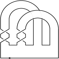
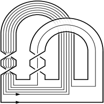
Figure 1. The fiber $\Sigma_{K}$ with the left-handed trefoil $K$ as boundary (left) and with the knot $\gamma_{p}\subset\Sigma_{K}$ (right, with $p=5$).

We point out that the left-handed trefoil knot $K$ is a genus $1$ knot, whose minimal genus Seifert surface (the fiber $\Sigma_{K}$, canonically defined up to isotopy) is a surface having boundary $K$ itself, illustrated in Figure 1 (left hand side). The fiber $\Sigma_{L}$ of $L$ is obtained from $\Sigma_{K}$ by removing any disk.

We will now identify now a family of simple closed curves, lying in $\Sigma_{L}$, that are homologous as elements of $H_{1}(S^{3}\setminus\nu L,{\mathbb{Z}})$, but not isotopic. We have several choices of simple closed curves lying in $\Sigma_{K}$. For sake of definiteness, we will consider the infinite family of knots defined as in the right hand side of Figure 1: the $p$-th element of the family has $p$ strands on the first twisted annulus and $1$ on the second, as represented in Figure 1 for the case of $p=5$ (in what follows we will always consider $p\geq 2$). Note that each $\gamma_{p}$ has a natural framing induced by the surface $\Sigma_{K}$.

It is not difficult to recognize that the knot denoted by $\gamma_{p}$ is in fact the torus knot $T(p,p+1)$. In fact, the two half-twists on the annulus act on the $p$ strands as illustrated in Figure 2 (for $p=5$).

Figure 2. The effect of the half-twist of the band on the strands, in two equivalent form.

Every strand under-crosses all the strands at its right, and we can represent this with both the braids of Figure 2 (the equivalence of the two braids can be checked with repeated application of the braid relations). We can now represent $\gamma_{p}$ as the composition of the two braids of Figure 2, plus the additional crossing of the $p$-th strand over the others (due to the passage on the second annulus of $\Sigma_{K}$). We obtain in this way the presentation of Figure 3 (left). Proceeding now as in Figure 3, we obtain a presentation of $\gamma_{p}$ as closure of a braid with $(p+1)$ strands that shows clearly that it is a torus knot, homologous to $p$ times the meridian and $(p+1)$ times the longitude of a standard torus in $S^{3}$. In particular, the example on the right hand side of Figure 1 is the torus knot $T(5,6)$.

       

Figure 3. A standard presentation of the torus knot through the isotopy indicated by the dashed line .

We claim that the linking number of $\gamma_{p}$ with $K$ is zero. In fact, by looking at the crossings of $\gamma_{p}$ and $K$ in Figure 1, we can see that the computation can be reduced to verifying that the sum of the signs of the crossings of each of the two strands of Figure 4 (left hand side) and $K$ equals zero, something that can be checked by direct computation as indicated in the Figure.

                 

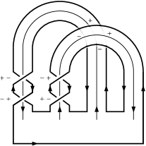
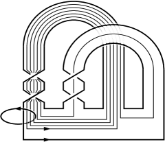
Figure 4. The crossing numbers of $\gamma_{p}$ (left) and the curve $\gamma_{5,3}\subset\Sigma_{L}$, together with the pair $K\cup M$ (right).

Now let’s consider the link $L$ and its fiber $\Sigma_{L}\subset\Sigma_{K}$. Without loss of generality, we can assume that the curves $\gamma_{p}$ are embedded in $\Sigma_{L}$, but in order to do so we need to specify how $M$ links $\gamma_{p}$. We will fix an integer $q\geq 1$, and consider the family of curves $\gamma_{p}$ for $p\geq q$. We can isotope $\gamma_{p}$ (in $\Sigma_{K}$) in such a way that $\gamma_{p}$ pierces with the first $q$ of its strands the spanning surface of $M$, as illustrated in the right hand side of Figure 4 (where $p=5$, $q=3$). We will denote by $\gamma_{p,q}$ the curve of $\Sigma_{L}$ thus obtained. In particular, for $q=1$, $M$ is isotopic (in $S^{3}\setminus\nu\gamma_{p,1}$) to a meridian of $\gamma_{p,1}$. As knots in $S^{3}$, we have $lk(\gamma_{p,q},M)=q$.

We want to make clear that, with the definition above, the surface $\Sigma_{L}$ contains, for all values of $q$, the entire family of curves $\{\gamma_{p,q}\}_{q,p\geq q}$.

We can define now a $3$-component link $L_{p,q}=L\cup\gamma_{p,q}$, which has linking matrix

(1) $$l_{p,q}=\left(\begin{array}[]{ccc}-&1&0\\ 1&-&q\\ 0&q&-\end{array}\right).$$

Observe that the linking matrix does not depend on $p$. As a consequence of this we have, in the homology of $S^{3}\setminus\nu L$, the following relation:

(2) $$[\gamma_{p,q}]=lk(\gamma_{p,q},K)[\mu(K)]+lk(\gamma_{p,q},M)[\mu(M)]=q[\mu(M)]\in H_{1}(S^{3}\setminus\nu L,{\mathbb{Z}}).$$

Although all the $\gamma_{p,q}$’s (for a fixed value of $q$) are homologous, they are quite clearly non isotopic, for different values of $p$, as knots in $S^{3}$ and, a fortiori, in $S^{3}\setminus\nu L$. We will exploit this fact in order to prove Theorem 1.1.

4. Construction of the symplectic link surgery manifold

The link surgery construction is a convenient method to translate some properties of knots and links to $4$-dimensional manifolds. In our case we will construct a symplectic manifold, homotopy equivalent to the elliptic surface $E(2)$, starting from the link $L$. Although not strictly necessary for the proof of Theorem 1.1, we will present the manifold in two different ways. First, as knot surgery for the knot $K$, and next as link surgery manifold for the link $L$. This pretty straightforward observation, true for any knot $K$, has some interest per se.

We will start with the standard definitions contained in [FS1] of a homotopy $E(n)$ associated with the knot $K$:

(3) $$E(n)_{K}=(E(n)\setminus\nu F)\cup_{T^{3}}S^{1}\times(S^{3}\setminus\nu K)=E(n)\#_{F=S^{1}\times C_{K}}S^{1}\times N_{K}$$

where the gluing map on the boundary $3$-torus identifies the elliptic fiber $F$ with $S^{1}\times\mu(K)$ and, reversing orientation, $\lambda(K)$ with the meridian circle to the elliptic fiber. In Equation 3 the $3$-manifold $N_{K}$ is the result of $0$-surgery of $S^{3}$ along $K$ and $C_{K}$ is the core of the Dehn filling (a curve isotopic to $\mu(K)$). The torus $S^{1}\times C_{K}$ has a canonical framing induced by the Dehn filling in $N_{K}$, while $F$ in $E(n)$ has a canonical framing induced from the fibration of $E(n)$. The fiber sum identifies the two tori and acts as complex conjugation on the normal bundles. We are interested in the case of $n=2$: we claim that $E(2)_{K}$ can be described as link surgery manifold over the link $L$, with the generalized definition introduced in [V1]. Precisely, we can construct an homotopy $E(2)$ starting from $L$ and the fibration of $S^{3}\setminus\nu L$ of fiber $\Sigma_{L}$ in the following way:

(4) $$\begin{array}[]{c}E(2)_{K}=\coprod_{i=1}^{2}(E(1)_{i}\setminus\nu F_{i})\cup_{T^{3}_{i}}S^{1}\times(S^{3}\setminus\nu L)=\\ \\ =E(1)_{1}\#_{F_{1}=S^{1}\times C_{K}}S^{1}\times N_{K}\#_{F_{2}=S^{1}\times C_{M}}E(1)_{2}.\end{array}$$

The gluing maps identify, on the first $3$-torus, $F_{1}$ with $S^{1}\times\mu(K)$ and the meridian of $F_{1}$ with $-\lambda(K)$ and, on the second $3$-torus, $F_{2}$ with $S^{1}\times\lambda(M)$ and the meridian of $F_{2}$ with $\mu(M)$. $C_{K}$ is again the core of the Dehn filling along $K$ and $C_{M}$ is the core of the trivial Dehn filling of the $\infty$-surgery along $M$ (a curve isotopic to $\lambda(M)$ itself). Note that, with this gluing prescription above, $\Sigma_{L}$ is naturally capped off with one disk section in each $(E(1)\setminus\nu F_{i})$. As $\lambda(M)$ is isotopic to $\mu(K)$ we have, up to isotopy, $C_{K}=C_{M}$ and $F_{1}=F_{2}=S^{1}\times C_{(\cdot)}$. The connection between the two definitions above comes by observing that, as $E(2)=E(1)\#_{F}E(1)$, we can think to $E(2)_{K}$ as obtained by fiber summing $E(1)$ to $E(1)_{K}$ along a copy of $F=S^{1}\times C_{K}$, which is exactly the definition of Equation 4. Note that the definitions of Equations 3 and 4 are equivalent also in the symplectic category.

The definition of $E(2)_{K}$ in Equation 4 shows the existence of two noteworthy homology classes of $E(2)_{K}$, images under the injective map

(5) $$i_{*}:H_{1}(S^{3}\setminus\nu L,{\mathbb{Z}})\longrightarrow H_{2}(S^{1}\times(S^{3}\setminus\nu L),{\mathbb{Z}})\longrightarrow H_{2}(E(2)_{K},{\mathbb{Z}})$$

of the two generators $[\mu(K)]$ and $[\mu(M)]$. The first one is identified with the homology class of $F$, while the second is the homology class of a kind of rim torus, identified with $S^{1}\times\mu(M)$, that we will denote by $R$. This class is primitive: in order to verify this, observe that the torus $R$ intersects once (with positive sign) the sphere obtained by capping the annulus spanning $M$ and pierced once by $K$ (representing the dual to the class $(0,1)\in H^{1}(S^{3}\setminus\nu L,{\mathbb{Z}})$) with one vanishing disks in each copy of $E(1)\setminus\nu F$. The class of $R$ has self-intersection $0$.

5. Infinitely many lagrangian tori

We are ready now, using the constructions of Sections 3 and 4, to exhibit a family of lagrangian tori that represents any multiple of the class of the rim torus $R$. Fix, as in Section 3, an integer $q\geq 1$ and pick the collection of curves $\gamma_{p,q}$ with $p\geq q$. The following holds true.

Lemma 5.1.

The images $R_{p,q}\subset E(2)_{K}$ of the tori $S^{1}\times\gamma_{p,q}\in S^{1}\times(S^{3}\setminus\nu L)$ define a family of lagrangian, framed tori representing the class $q[R]$.

Proof: The homology class of these tori is given, by Equation 2, by the formula

(6) $$\begin{array}[]{c}[R_{p,q}]=i_{*}[\gamma_{p,q}]=lk(\gamma_{p,q},K)i_{*}[\mu(K)]+lk(\gamma_{p,q},M)i_{*}[\mu(M)]=\\ \\ =q[R]\in H_{2}(E(2)_{K},{\mathbb{Z}}).\end{array}$$

The elements of the infinite collection of tori $R_{p,q}$, with $p\geq q$, is therefore homologous to $q$ copies of $R$. As the knot $K$ is fibered, the closed $3$-manifold $N_{K}$ is fibered too, with fiber the surface $\Sigma_{L}$ capped off with two disks. The fiber sum presentation of Equation 4, scaling suitably the symplectic forms to obtain matching volumes on the gluing tori, shows that $E(2)_{K}$ admits a symplectic structure that, on the interior of $S^{1}\times N_{K}\setminus\nu(S^{1}\times C_{K}\cup S^{1}\times C_{M})=S^{1}\times(S^{3}\setminus\nu L)$, coincides with the restriction of a standard symplectic form on $S^{1}\times N_{K}$, namely $\alpha\wedge dt+\epsilon\beta$, where $\alpha$ is a closed $1$-form on $N_{K}$ determined up to isotopy by the fibration of $N_{K}$ and $\beta$ is a closed $2$-form on $N_{K}$ restricting to a volume form on each fiber. The tori $S^{1}\times\gamma_{p,q}$ embed in $S^{1}\times N_{K}$ and are lagrangian with respect to its symplectic structure, as the tangent space in each point is spanned by $\frac{\partial}{\partial t}$ and by a vector tangent to the fiber, and therefore lying in the kernel of $\alpha$. Consequently, the tori $R_{p,q}$ are lagrangian and have a canonical framing induced from $\Sigma_{L}$; this framing coincides with the lagrangian framing, as the tori obtained by pushing off $\gamma_{p,q}$ along $\Sigma_{L}$ are lagrangian. This completes the proof of the Lemma. Q.e.d.

Lemma 5.1 asserts that the tori $R_{p,q}$, for a fixed value of $q$, are images of homotopic lagrangian embeddings of $T^{2}$ in $E(2)_{K}$. Our goal is now to show that these tori are not isotopic. In order to do so, we can define the family of (symplectic) manifolds

(7) $$X_{p,q}=E(1)\#_{F=R_{p,q}}E(2)_{K}.$$

The definition of the fiber sum depends a priori on the choice of the framing for $R_{p,q}$, determining (with a marking of the tori) the gluing map for the boundary $3$-tori. Anyhow, any orientation preserving self-diffeomorphism of $\partial(E(1)\setminus\nu F)$ extends to $(E(1)\setminus\nu F)$ (see [GS]): different choices of the framing or marking lead therefore to the same smooth manifold, namely $X_{p,q}$ depends only on the isotopy class of $R_{p,q}$. More is actually true, namely the smooth structure of $X_{p,q}$ depends only the diffeomorphism type of the pair $(E(2)_{K},R_{p,q})$. Our goal is to distinguish different smooth structures, for different values of $p$, by computing the Seiberg-Witten polynomial of $X_{p,q}$. In order to do so, we start with the following

Proposition 5.2.

Consider the manifold $X_{p,q}=E(1)\#_{F=R_{p,q}}E(2)_{K}$ and the $3$-component link $L_{p,q}=K\cup M\cup\gamma_{p,q}$. The manifold $X_{p,q}$ is diffeomorphic to the link surgery manifold $E(3)_{L_{p,q}}$.

Proof: The manifolds $X_{p,q}$ and $E(3)_{L_{p,q}}$ can both be written, as smooth manifolds, as

(8) $$\coprod_{i=1}^{3}(E(1)\setminus\nu F)\cup_{T^{3}_{i}}S^{1}\times(S^{3}\setminus L_{p,q}),$$

where the gluing maps on the boundary $3$-tori are defined in different ways for the two manifolds. However, because of the aforementioned extension property of the self-diffeomorphisms of $\partial(E(1)\setminus\nu F)$, the choice of the gluing maps does not affect the smooth structure of the resulting manifold. Q.e.d. Proposition 5.2 allows us to apply the following Lemma of Fintushel-Stern ([FS1]).

Lemma 5.3.

Let $\Delta^{s}_{p,q}(x,y,t)$ be the symmetrized Alexander polynomial of the link $L_{p,q}=K\cup M\cup\gamma_{p,q}$. Then the Seiberg-Witten polynomial of $X_{p,q}$ is given by

(9) $$SW_{X_{p,q}}=\Delta^{s}_{p,q}(x^{2},y^{2},t^{2})$$

where we identify $x,y,t$ with (the Poincaré dual of) the images of $S^{1}\times\mu(K),S^{1}\times\mu(M),S^{1}\times\mu(\gamma_{p,q})$ respectively.

Note that, as the relative Seiberg-Witten polynomial of $(E(1),F)$ is just equal to $1$, the polynomial of Equation 9 is in fact the relative Seiberg-Witten polynomial of $(E(2)_{K},R_{p,q})$ - see [MT] for a discussion of the invariants from this point of view. We will use this result in the next section to prove our main Theorem.

6. Proof of the main theorem

In order to prove Theorem 1.1 we could attempt to compute, using Lemma 5.3, the SW polynomial of $X_{p,q}$ for each value of $p$ and use the result to distinguish the smooth structure for different values of $p$ and, with that, the isotopy class of the torus $R_{p,q}$. Conceptually, the computation of the Alexander polynomial of $L_{p,q}$ does not present any difficulty, but obtaining a general formula is practically not viable. Moreover, even when this is done, while comparing the SW polynomial of two manifolds, we would need to show that there is no change of basis in the second cohomology group transforming one polynomial in the other, compare with the discussion in [V2].

For this reason, we will be content with a weaker result, that is anyhow sufficient to prove Theorem 1.1 (even in its stronger form for diffeomorphisms of pairs)

Theorem 6.1.

For any choice of $q\geq 1$ the family of manifolds $\{X_{p,q}\}_{p\geq q}$ contains infinitely many pairwise non-diffeomorphic manifolds.

Proof: In order to prove the statement it is enough to show that the number of basic classes of $X_{p,q}$, that we will denote by $\beta_{p,q}$, satisfies the condition $lim_{p}\beta_{p,q}=\infty$. As all the manifolds $X_{p,q}$ have a finite number of basic classes, this implies that infinitely many components of the family $\{X_{p,q}\}_{p\geq q}$ are distinguished by the SW polynomial. To start we can observe that $\beta_{p,q}$ is the same as the number of nonzero terms of $\Delta_{p,q}(x,y,t)$ (symmetrization is irrelevant here). The latter number, moreover, is bounded below by the number of nonzero terms of any specialization of the polynomial, so we will make our life simpler by considering specializations of $\Delta_{p,q}(x,y,t)$. We have the following Lemma.

Lemma 6.2.

The number of nonzero terms of the Alexander polynomial $\Delta_{p,q}(x,y,t)$ of $L_{p,q}$ is bounded below by the number of nonzero terms of the polynomial (written here in quotient form)

(10) $$P_{p,q}(t)=\frac{(1-t^{q})(1-(t^{p+1})^{p})}{(1-t^{p})(1-t^{p+1})}.$$

Proof: The number of nonzero terms of $\Delta_{p,q}(x,y,t)$ is bounded below by the number of nonzero terms of $\Delta_{p,q}(1,y,t)$. This specialization of the Alexander polynomial can be computed using the Torres formula (see e.g., [Tu]) to get

(11) $$\Delta_{p,q}(1,y,t)=(y^{lk(M,K)}t^{lk(\gamma_{p,q},K)}-1)\Delta_{\gamma_{p,q}\cup M}(y,t)=(y-1)\Delta_{\gamma_{p,q}\cup M}(y,t).$$

Let’s consider first the case of $q=1$. In this case, $\gamma_{p,1}\cup M$ is a pair given by the torus knot and its meridian or, which is the same, its $(0,1)$-cable. As such we can represent it as result of splicing $\gamma_{p}$ with the generalized Hopf link (the “necklace”) $H$ (with $3$ components), along a component $H_{2}$. The Alexander polynomial of $H$ is given, as easily checked, by $\Delta_{H}(u,v,w)=(u-1)$. Applying the splicing formula of Theorem 5.3 of [EN] we find that $\Delta_{\gamma_{p,1}\cup M}(y,t)=\Delta_{\gamma_{p}}(t)$, where the latter is the Alexander polynomial of the torus knot $T(p,p+1)$, namely

(12) $$\Delta_{\gamma_{p}}(t)=\frac{(1-t)(1-(t^{p+1})^{p})}{(1-t^{p})(1-t^{p+1})}.$$

This exactly the polynomial $P_{p,1}(t)$ of Equation 10 and it should be clear at this point, by looking at Equation 11, that the statement of the Lemma holds true for $q=1$. To prove the general case, let’s write

(13) $$\Delta_{\gamma_{p,q}\cup M}(y,t)=\sum_{k}a_{k,p,q}(y)t^{k},$$

where the Laurent polynomials $a_{k,p,q}(y)$ are defined by this identity. We can write Equation 11 in the form

(14) $$\Delta_{p,q}(1,y,t)=\sum_{k}(y-1)a_{k,p,q}(y)t^{k}.$$

Consider the set of coefficients $(y-1)a_{k,p,q}(y)$ of this Laurent polynomial of the variable $t$. The number of coefficients that are nonzero is bounded below by the number of terms $a_{k,p,q}(1)$ that are nonzero. By the definition contained in Equation 13, the value of $a_{k,p,q}(1)$ is determined by the Equation

(15) $$\sum_{k}a_{k,p,q}(1)t^{k}=\Delta_{\gamma_{p,q}\cup M}(1,t)=\frac{t^{lk(\gamma_{p,q},M)}-1}{t-1}\Delta_{\gamma_{p}}(t)=\frac{t^{q}-1}{t-1}\Delta_{\gamma_{p}}(t),$$

where to get the last expression we used again Torres formula. By looking at Equation 12 we see that this last polynomial is exactly the polynomial $P_{p,q}(t)$ of Equation 10. Q.e.d.

The formula of Equation 10 tells us that $\beta_{p,q}$ is bounded below by the number of nonzero terms in the polynomial $P_{p,q}(t)$. Concerning this polynomial, we have the following result:

Lemma 6.3.

The number of nonzero terms of the polynomial $P_{p,q}(t)$, with $p\geq q$, is bounded below by $p-q+1$.

Proof: The proof of this statement follows by a fairly simple argument. First, we can rewrite, in ${\mathbb{Z}}[[t]]$,

(16) $$\begin{array}[]{c}P_{p,q}(t)=\frac{(1+t^{p+1}+...+t^{(p-1)(p+1)})(1-t^{q})}{1-t^{p}}=\\ \\ =\frac{1-t^{q}+t^{p+1}-t^{p+1+q}+...+t^{(p-1)(p+1)}-t^{(p-1)(p+1)+q}}{1-t^{p}}=\\ \\ =(1-t^{q}+t^{p+1}-t^{p+1+q}+...+t^{(p-1)(p+1)}-t^{(p-1)(p+1)+q})(1+t^{p}+t^{2p}+...).\end{array}$$

The product of the polynomial and the formal power series above is in fact a polynomial, and we claim that it contains all the $p-q+1$ terms of the form

(17) $$t^{(q-1)(p+1)},t^{(q-1)(p+1)+p},...,t^{(q-1)(p+1)+(p-q-1)p},t^{(q-1)(p+1)+(p-q)p}.$$

In order to prove so, observe first that, as $0\leq(q-1)\leq(p-1)$, the polynomial in the second line of Equation 16 contains the term $t^{(q-1)(p+1)}$ with coefficient equal to $1$. Therefore we obtain, with coefficient equal to $1$, all the terms of Equation 17 by multiplying the term $t^{(q-1)(p+1)}$ by the first $(p-q+1)$ terms of the formal power series (plus an infinite series of other terms that, in fact, will get canceled). Next, considering the fact that the power series has all terms with positive coefficients, the only possibility for the terms $t^{(q-1)(p+1)+np}$, $0\leq n\leq(p-q)$ to be canceled is that there exists a pair $k,l\in{\mathbb{N}}$, with $0\leq l\leq(p-1)$, such that

(18) $$(q-1)(p+1)+np=kp+l(p+1)+q$$

(roughly speaking, the power of $t^{l(p+1)+q}\cdot t^{kp}$, appearing with a negative sign, must equal the power of $t^{(q-1)(p+1)+np}$). Remember that, in this equation, $p$ and $q$ are fixed. Equation 18 means that, mod $p$, we must have $l+1=0$. As $0\leq l\leq(p-1)$, the only solution to this condition is $l=(p-1)$. With this value of $l$, Equation 18 becomes

(19) $$(q-1)p+np=kp+p^{2}.$$

The smallest value of $n$ for which this equation holds true is when $k=0$, for which $n=p-q+1$, namely none of the terms in Equation 17 gets canceled, as claimed (while the higher terms get canceled, as they should). With similar considerations it is possible to show that the coefficient of these terms is exactly equal to $1$, but we will omit the proof (as it has no implications to our result). Q.e.d. (Note that the estimate contained in Proposition 6.3 is quite rough, and probably without much effort a precise value could be obtained, but this result would be irrelevant in our discussion).

Proposition 6.3 implies that $\lim_{p\rightarrow\infty}\beta_{p}\geq\lim_{p\rightarrow\infty}(p-q+1)=\infty$, and thus completes the proof of Theorem 6.1 and, with that, Theorem 1.1. Q.e.d.

References

- [A] V.Arnol’d, First Steps in Symplectic Topology, Russian Math.Surveys 41(6), 1-21 (1986) .
- [ADK] D.Auroux, S.Donaldson, L.Katzarkov, Luttinger Surgery Along Lagrangian Tori and Non-Isotopy for Singular Symplectic Plane Curves, Math. Ann. 326, no. 1, 185–203 (2003).
- [EN] D.Eisenbud, W.Neumann, Three Dimensional Link Theory and Invariants of Plane Curve Singularities, Annals of Mathematics Studies 110 (1985).
- [ElP1] Y.Eliashberg, L.Polterovich, Unknottedness of Lagrangian Surfaces in Symplectic -manifolds, Internat.Math.Res.Notices 11, 295-301 (1993).
- [ElP2] Y.Eliashberg, L.Polterovich, Local Lagrangian -knots are trivial, Ann. of Math. (2) 144, 61-76 (1996).
- [ElP3] Y.Eliashberg, L.Polterovich, The Problem of Lagrangian Knots in Four-Manifolds, Geometric Topology. Proceedings of the 1993 Georgia International Topology Conference (W.H.Kazez, ed.), International Press, 313-327 (1997).
- [EtP] T.Etgü, B.D.Park, Nonisotopic Symplectic Tori in the Same Homology Class, Trans. Amer. Math. Soc. 356, no. 9, 3739-3750 (2004).
- [FS1] R.Fintushel, R.Stern, Knots, Links and -manifolds, Inv.Math. 134, 363-400 (1998).
- [FS2] R.Fintushel, R.Stern, Symplectic Surfaces in a Fixed Homology Class, J. Differential Geom. 52, 203-222 (1999).
- [G] R.Gompf, A New Construction of Symplectic Manifolds, Ann. of Math. 142, 527-595 (1995).
- [GS] R.Gompf, A.Stipsicz, 4-Manifolds and Kirby Calculus, Graduate Studies in Mathematics (vol. 20) AMS (1999).
- [L] K.M.Luttinger, Lagrangian Tori in , J.Diff.Geom. 42, 220-228 (1995).
- [LS] F.Lalonde, J.-C.Sikorav, Sous-variétés lagrangiennes et lagrangiennes exactes des fibrés cotangents, Comment. Math. Helv. 66, 18-33 (1991).
- [MT] C.McMullen, C.Taubes, 4-Manifolds with Inequivalent Symplectic Forms and 3-Manifolds with Inequivalent Fibrations, Math.Res.Lett. 6, 681-696 (1999).
- [Se1] P.Seidel, Lagrangian Two-spheres can be Symplectically Knotted, J. Differential Geom. 52, 145-171 (1999).
- [Se2] P.Seidel Graded Lagrangian Submanifolds, Bull. Soc. Math. France 128, 103-149 (2000).
- [Sm] I.Smith, Symplectic Submanifolds from Surface Fibrations, Pacif.Jour.Math. 198, 197-206 (2001).
- [Ti] G.Tian, Symplectic isotopy in four dimension, First International Congress of Chinese Mathematicians (Beijing, 1998), AMS/IP Stud. Adv. Math., 20, 143-147 (2001).
- [Tu] V.Turaev, Reidemeister Torsion in Knot Theory, Russian Math.Surveys 41(1), 97-147 (1986).
- [V1] S.Vidussi, Smooth Structure of Some Symplectic Surface, Michigan Math.J. 49, 325-330 (2001).
- [V2] S.Vidussi, Nonisotopic Symplectic Tori in the Fiber Class of Elliptic Surfaces, J. Symplectic Geom. 2, no. 2, 207-218 (2004).